
Application of General Linear Models (GLM) to Assess Nodule Abundance Based on a Photographic Survey (Case Study from IOM Area, Pacific Ocean)


Abstract
:1. Introduction
2. Research Objective
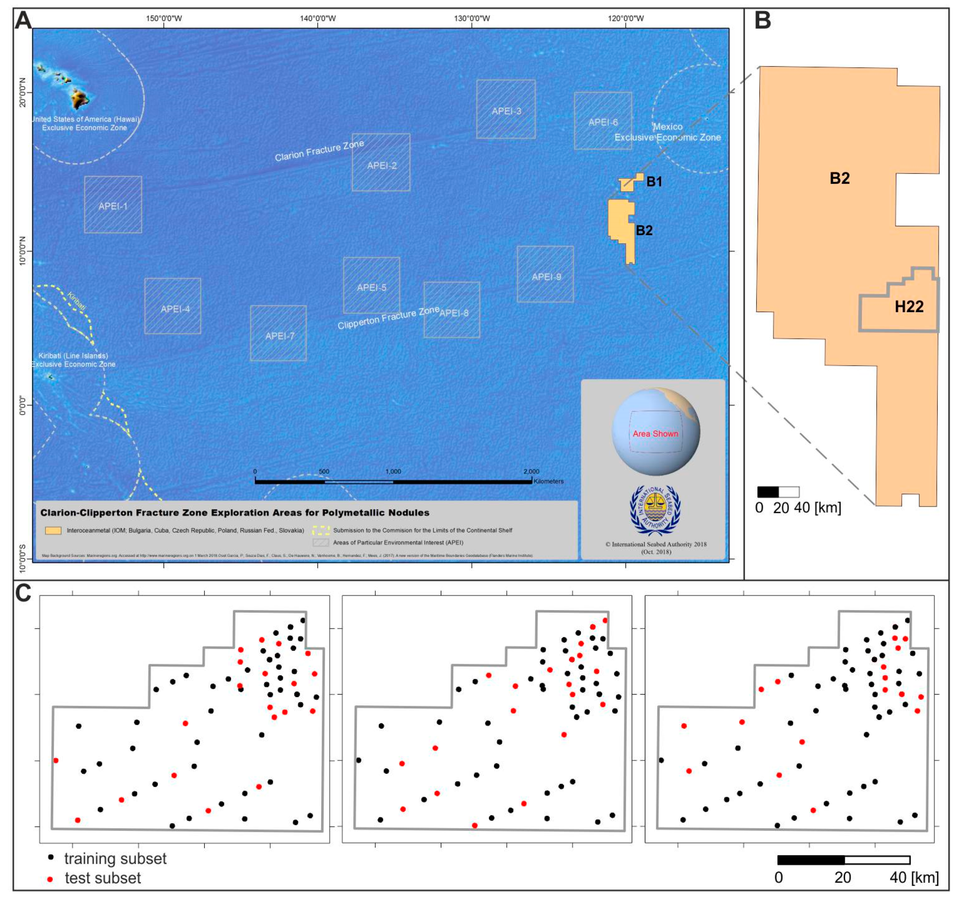
3. Materials
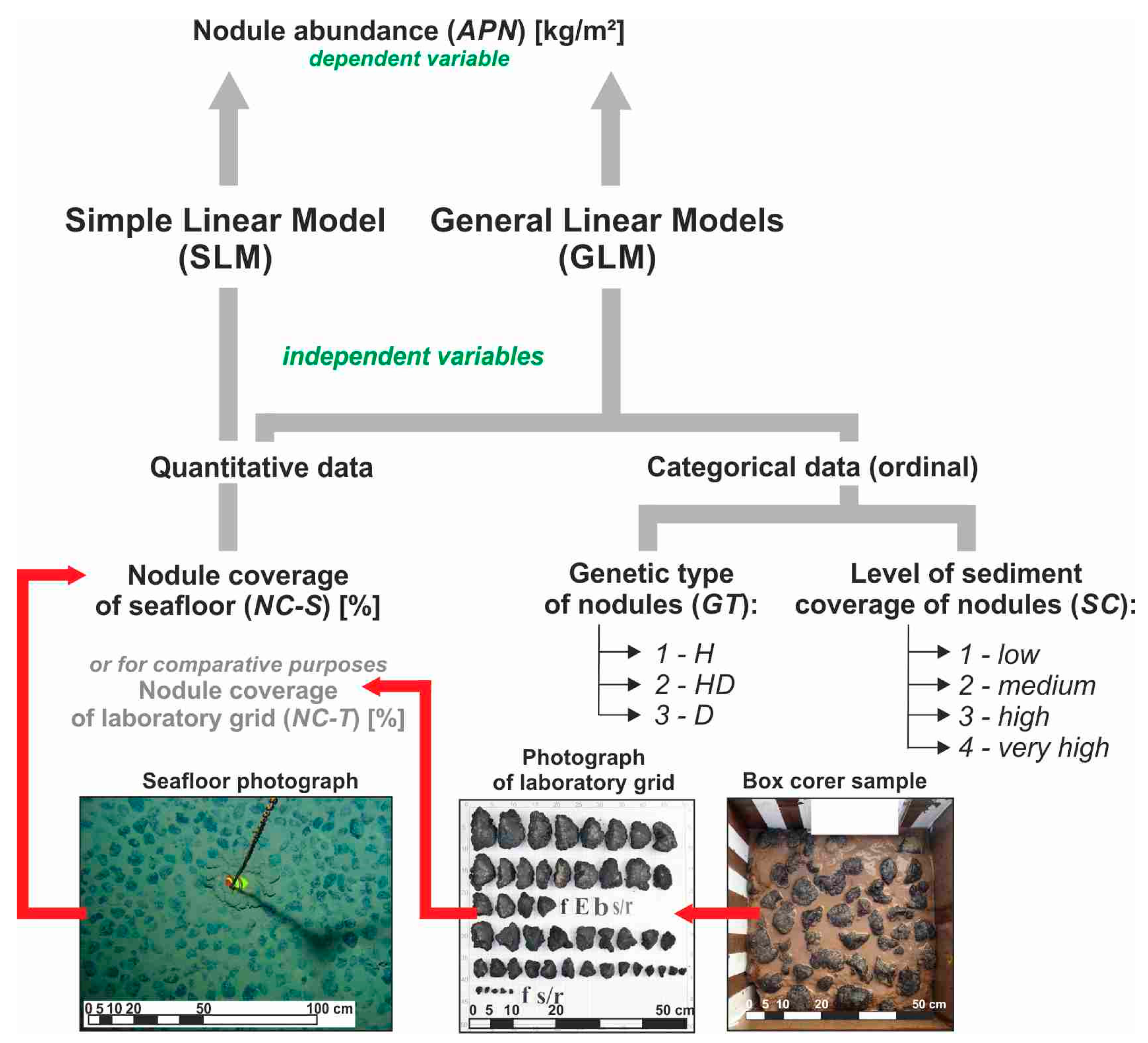
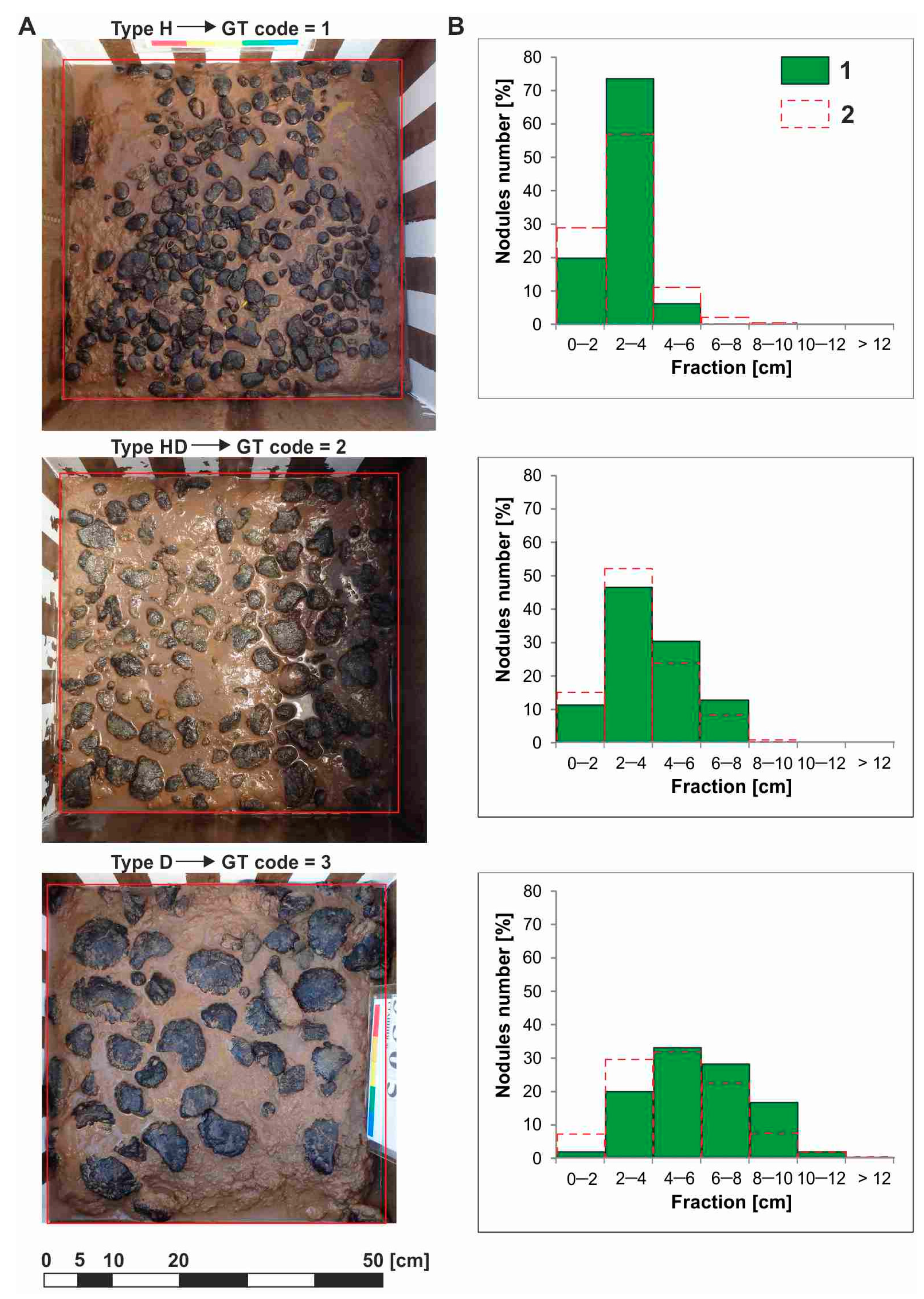
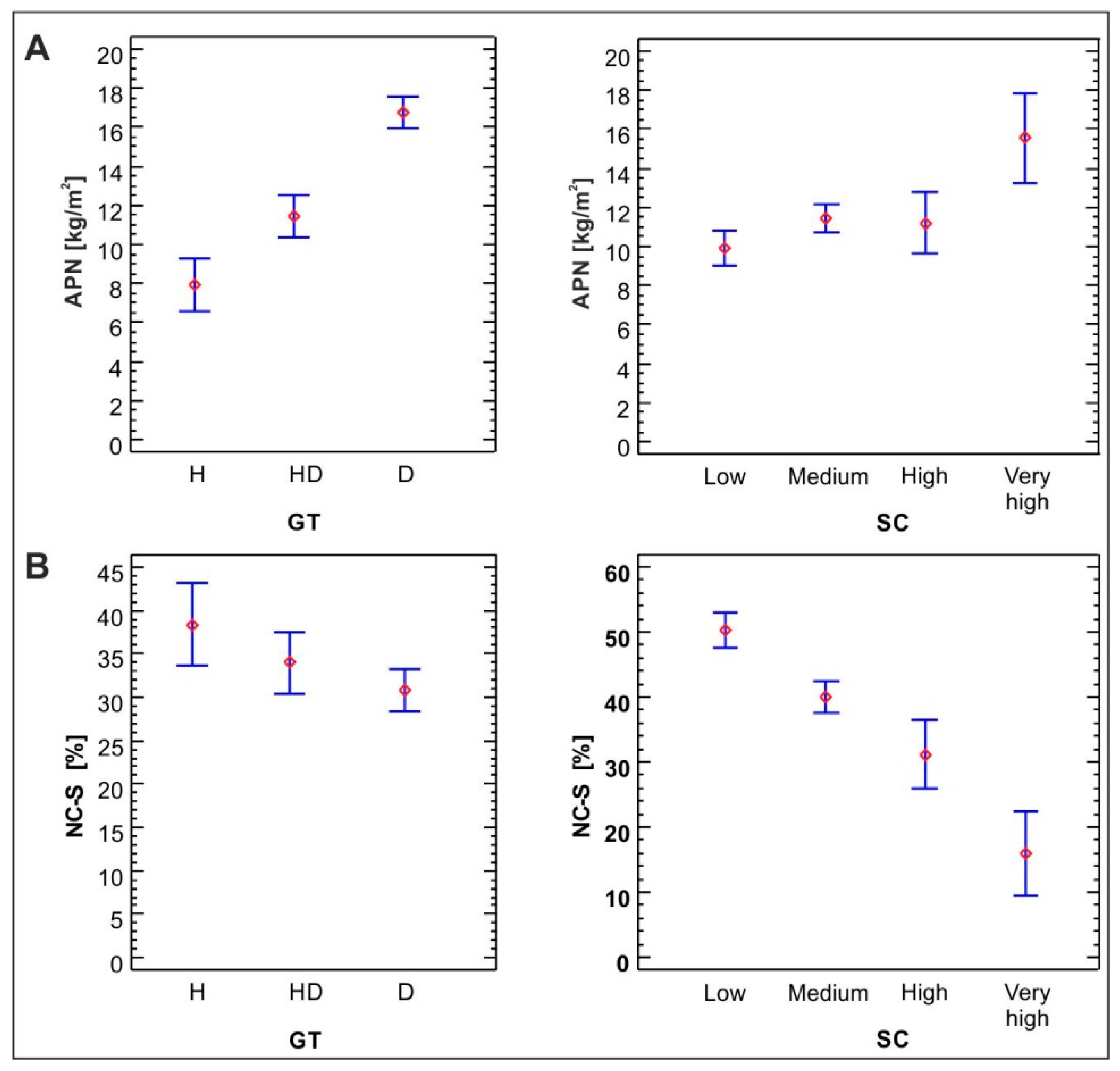
- HD (hydrogenetic-diagenetic)—nodules intermediate in size (by convention, from 3 to 6 cm in diameter) with a smooth upper surface and a rough lower surface, predominantly ellipsoidal, flattened, and plate-shaped;
- D (diagenetic)—large nodules, 6–12 cm in diameter, predominantly discoidal and ellipsoidal in shape and with rough surfaces.
4. Methods
- The adjusted coefficient of determination expresses the percentage of the variability in the dependent variable, which has been explained by the fitted model, ranging from 0% (lack of the dependency) to 100% (ideal, full relationship), adjusted for the number of coefficients in the model:where n—count of data, p—the number of estimated model coefficients, —theoretical value of the dependent variable Y determined from the model equation for the observation “i”, —empirical value of the dependent variable Y for the observations “i”, —arithmetic mean of the empirical values of the dependent variable Y.
- The standard (prediction) error of estimation (SEE) characterizing the average scatter of the measured values of the dependent variable in the regression model:
- The mean absolute error (MAE) characterizing the mean absolute deviation of the measured Y values from the values indicated by the model:
- Mean percentage error (MPE):
- Mean absolute percentage error (MAPE):
5. Results and Discussion
- GLM:
- SLM:
- Determining the statistical significance of the linear relationship between the nodule abundance predicted from the models (for the training data) with the real nodule abundance in the test sets (using p-value) and the strength of this relationship using the adjusted coefficient of determination );
- Determination of the arithmetic mean (MD) and mean absolute difference (MAD) between the nodule abundance predicted from the model and found in the test sets.
6. Conclusions
Author Contributions
Funding
Institutional Review Board Statement
Informed Consent Statement
Data Availability Statement
Acknowledgments
Conflicts of Interest
References
- Hein, J.R.; Mizell, K.; Koschinsky, A.; Conrad, T.A. Deep-ocean mineral deposits as a source of critical metals for high- and green-technology applications: Comparison with land-based resources. Ore Geol. Rev. 2013, 51, 1–14. [Google Scholar] [CrossRef]
- Petersen, S.; Krätschell, A.; Augustin, N.; Jamieson, J.; Hein, J.R.; Hannington, M.D. News from the seabed—Geological characteristics and resource potential of deep-sea mineral resources. Mar. Policy 2016, 70, 175–187. [Google Scholar] [CrossRef]
- Milinovic, J.; Rodrigues, F.J.L.; Barriga, F.J.A.S.; Murton, B.J. Ocean-floor sediments as a resource of rare earth elements: An overview of recently studied sites. Minerals 2021, 11, 142. [Google Scholar] [CrossRef]
- Toro, N.; Robles, P.; Jeldres, R.I. Seabed mineral resources, an alternative for the future of renewable energy: A critical review. Ore Geol. Rev. 2020, 126, 103699. [Google Scholar] [CrossRef]
- Toro, N.; Jeldres, R.I.; Órdenes, J.A.; Robles, P.; Navarra, A. Manganese nodules in chile, an alternative for the production of co and mn in the future—A review. Minerals 2020, 10, 674. [Google Scholar] [CrossRef]
- Watzel, R.; Rühlemann, C.; Vink, A. Mining mineral resources from the seabed: Opportunities and challenges. Mar. Policy 2020, 114, 103828. [Google Scholar] [CrossRef]
- Hein, J.R.; Koschinsky, A.; Kuhn, T. Deep-ocean polymetallic nodules as a resource for critical materials. Nat. Rev. Earth Environ. 2020, 1, 158–169. [Google Scholar] [CrossRef]
- Abramowski, T.; Stoyanova, V. Deep-Sea Polymetallic Nodules: Renewed Interest as Resources for Environmentally Sustainable Development. In Proceedings of the SGEM2012 Conference, Albena, Bulgaria, 17–23 June 2012; Volume 1, pp. 515–522. [Google Scholar] [CrossRef]
- Pérez, K.; Villegas, Á.; Saldaña, M.; Jeldres, R.I.; González, J.; Toro, N. Initial investigation into the leaching of manganese from nodules at room temperature with the use of sulfuric acid and the addition of foundry slag—Part II. Sep. Sci. Technol. 2021, 56, 389–394. [Google Scholar] [CrossRef]
- Toro, N.; Saldaña, M.; Castillo, J.; Higuera, F.; Acosta, R. Leaching of manganese from marine nodules at room temperature with the use of sulfuric acid and the addition of tailings. Minerals 2019, 9, 289. [Google Scholar] [CrossRef] [Green Version]
- Usui, A.; Hino, H.; Suzushima, D.; Tomioka, N.; Suzuki, Y.; Sunamura, M.; Kato, S.; Kashiwabara, T.; Kikuchi, S.; Uramoto, G.-I.; et al. Modern precipitation of hydrogenetic ferromanganese minerals during on-site 15-year exposure tests. Sci. Rep. 2020, 10, 1–10. [Google Scholar] [CrossRef] [Green Version]
- Usui, A.; Nishi, K.; Sato, H.; Nakasato, Y.; Thornton, B.; Kashiwabara, T.; Tokumaru, A.; Sakaguchi, A.; Yamaoka, K.; Kato, S.; et al. Continuous growth of hydrogenetic ferromanganese crusts since 17 Myr ago on Takuyo-Daigo Seamount, NW Pacific, at water depths of 800–5500 m. Ore Geol. Rev. 2017, 87, 71–87. [Google Scholar] [CrossRef] [Green Version]
- Zawadzki, D.; Maciąg, Ł.; Abramowski, T.; McCartney, K. Fractionation trends and variability of rare earth elements and selected critical metals in pelagic sediment from abyssal basin of NE Pacific (clarion-clipperton fracture zone). Minerals 2020, 10, 320. [Google Scholar] [CrossRef] [Green Version]
- Abramowski, T.; Urbanek, M.; Baláž, P. Structural Economic assessment of polymetallic nodules mining project with updates to present market conditions. Minerals 2021, 11, 311. [Google Scholar] [CrossRef]
- Parianos, J.; Lipton, I.; Nimmo, M. Aspects of estimation and reporting of mineral resources of seabed polymetallic nodules: A contemporaneous case study. Minerals 2021, 11, 200. [Google Scholar] [CrossRef]
- Sharma, R. Deep-sea mining: Current status and future considerations. In Deep-Sea Mining: Resource Potential, Technical and Environmental Considerations; Sharma, R., Ed.; Springer Science and Business Media LLC: Berlin, Germany, 2017; pp. 3–21. [Google Scholar]
- Abramovski, T.; Stefanova, V.P.; Causse, R.; Romanchuk, A. Technologies for the processing of polymetal-lic nodules from clarion clipperton zone in the Pacific Ocean. J. Chem. Technol. Metal. 2017, 52, 258–269. [Google Scholar]
- Vu, N.H.; Kristianová, E.; Dvořák, P.; Abramowski, T.; Dreiseitl, I.; Adrysheva, A. Modified leach residues from processing deep-sea nodules as effective heavy metals adsorbents. Metals 2019, 9, 472. [Google Scholar] [CrossRef] [Green Version]
- Clarion-Clipperton Fracture Zone Exploration Areas for Polymetallic Nodules (Interoceanmetal Joint Organization). Available online: https://www.isa.org.jm/map/interoceanmetal-joint-organization (accessed on 31 October 2020).
- Mucha, J.; Wasilewska-Błaszczyk, M. Estimation accuracy and classification of polymetallic nodule resources based on classical sampling supported by seafloor photography (Pacific Ocean, Clarion-Clipperton Fracture Zone, IOM Area). Minerals 2020, 10, 263. [Google Scholar] [CrossRef] [Green Version]
- Sterk, R.; Stein, J.K. Seabed mineral deposits: An overview of sampling techniques and future developments. In Proceedings of the Deep Sea Mining Summit, Aberdeen, Scotland, 9–10 February 2015; p. 29. [Google Scholar]
- Schoening, T.; Jones, D.O.B.; Greinert, J. Compact-Morphology-based poly-metallic Nodule Delineation. Sci. Rep. 2017, 7, 1–12. [Google Scholar] [CrossRef] [PubMed]
- Felix, D. Some problems in making nodule abundance estimates from seafloor photographs. Mar. Min. 1980, 2, 293–302. [Google Scholar]
- Handa, K.; Tsurusaki, K. Manganese nodules: Relationship between Coverage and Abundance in the Northern Part of Central Pacific Basin. Geol. Surv. Jpn. 1981, 15, 184–217. [Google Scholar]
- Lipton, I.; Nimmo, M.; Stevenson, I. NORI Area D Clarion Clipperton Zone Mineral Resource Estimate. Deep Green Metals Inc. Pacific Ocean; AMC Project 318010; AMC Consultants Pty Ltd.: Perth, WA, Australia, 2019. [Google Scholar]
- Jie, W.L.; Kalyan, B.; Chitre, M.; Vishnu, H. Polymetallic nodules abundance estimation using sidescan sonar: A quantitative approach using artificial neural network. OCEANS 2017—Aberdeen 2017, 1–6. [Google Scholar] [CrossRef]
- Yoo, C.M.; Joo, J.; Lee, S.H.; Ko, Y.; Chi, S.-B.; Kim, H.J.; Seo, I.; Hyeong, K. Resource assessment of polymetallic nodules using acoustic backscatter intensity data from the Korean exploration Area, Northeastern Equatorial Pacific. Ocean Sci. J. 2018, 53, 381–394. [Google Scholar] [CrossRef]
- Wasilewska-Błaszczyk, M.; Mucha, J. Possibilities and limitations of the use of seafloor photographs for estimating polymetallic nodule resources—Case study from IOM Area, Pacific Ocean. Minerals 2020, 10, 1123. [Google Scholar] [CrossRef]
- Kuhn, T.; Rathke, M. Report on Visual Data Acquisition in the Field and Interpretation for SMnN; Blue Mining Project; Blue Mining Deliverable D1.31; European Commission Seventh Framework Programme, 2017; p. 34. Available online: https://bluemining.eu/download/project_results/public_reports/BLUE-MINING-D1.31b-Final-Report-on-visual-data-acquisition-in-the-field-and-interpretation-for-SMnN.pdf (accessed on 12 March 2021).
- Jung, M.Y.; Kim, I.K.; Kang, J.K. Analysis of manganese nodule abundance in KODOS Area. Econ. Environ. Geol. 1995, 28, 429–437. [Google Scholar]
- Park, C.-Y.; Park, S.-H.; Kim, C.-W.; Kang, J.-K.; Kim, K.-H. An image analysis technique for exploration of manganese nodules. Mar. Georesour. Geotechnol. 1999, 17, 371–386. [Google Scholar] [CrossRef]
- Tsune, A. Effects of size distribution of deep-sea polymetallic nodules on the estimation of abundance obtained from seafloor photographs using conventional formulae. In Proceedings of the Eleventh OceanMining and Gas Hydrates Symposium, Big Island, HI, USA, 21–27 June 2015; International Society ofOffshore and Polar Engineers: Kona, HI, USA, 2015; p. 7. [Google Scholar]
- Sharma, R.; Khadge, N.; Sankar, S.J. Assessing the distribution and abundance of seabed minerals from seafloor photographic data in the Central Indian Ocean Basin. Int. J. Remote. Sens. 2012, 34, 1691–1706. [Google Scholar] [CrossRef]
- Balaz, P.; Krawcewicz, A.; Abramowski, T. 30 Years of Deep Seabed Exploration; Interoceanmetal Joint Organization: Szczecin, Poland, 2017. [Google Scholar]
- Dreiseitl, I. Deep Sea Exploration for Metal Reserves—Objectives, Methods and Look into the Future. In Deep See Mining Value Chain: Organization, Technology and Development; Abramowski, T., Ed.; Interoceanmetal Join Organization: Szczecin, Poland, 2016; pp. 105–117. [Google Scholar]
- Statgraphics; (Version Centurion XVII); Statpoint Technologies, Inc.: Warrenton, VA, USA.
- Kotliński, R. Relationships between Nodule Genesis and Topography in the Eastern Area of the C-C Region. In Establishment of A Geological Model of Polymetallic Nodule Deposits in the Clarion-Clipperton Fracture Zone of The Equatorial North Pacific Ocean. Proceedings of the International Seabed Authority’s Workshop, Nadi, Fiji, 13–20 May 2003; International Seabed Authority: Kingston, Jamaica, 2009; pp. 203–221. [Google Scholar]
- A Geological Model of Polymetallic Nodule Deposits in the Clarion-Clipperton Fracture Zone; ISA Technical Study; Technical Study: No. 6; ISA, International Seabed Authority: Kingston, Jamaica, 2010; p. 211.
- Dobson, A.J.; Barnett, A.G. An Introduction to Generalized Linear Models; CRC Press: Boca Raton, FL, USA, 2008. [Google Scholar]
- LaRose, D.T. Data Mining Methods and Models; Wiley: Hoboken, NJ, USA, 2005. [Google Scholar]
- Benoit, K. Linear Regression Models with Logarithmic Transformations. Available online: http://www.kenbenoit.net/courses/ME104/logmodels2.pdf (accessed on 15 June 2020).
- Chilès, J.-P.; Delfiner, P. Geostatistics: Modeling Spatial Uncertainty, 2nd ed.; John Wiley & Sons: Noboken, NJ, USA, 2009. [Google Scholar]


| Statistics | APN (kg/m2) | NC-S (%) |
|---|---|---|
| Count | 68 | 68 |
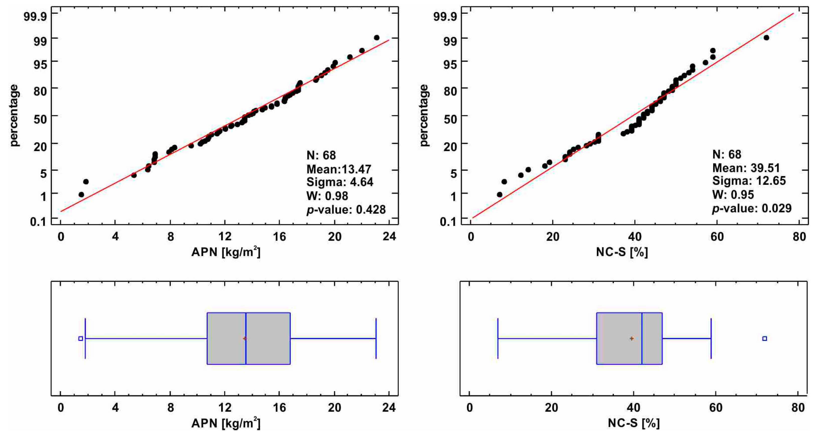
| Average | 13.47 | 39.51 |
| Median | 13.55 | 42.0 |
| 20% Trimmed mean | 13.81 | 41.16 |
| Standard deviation | 4.64 | 12.65 |
| Coeff. of variation | 34.4% | 32.0% |
| Minimum | 1.5 | 7.0 |
| Maximum | 23.1 | 72.0 |
| Range | 21.6 | 65.0 |
| Stnd. skewness | −1.30 | −1.89 |
| Stnd. kurtosis | −0.10 | 0.77 |
| p-value (Shapiro–Wilk test) | 0.428 | 0.029 |
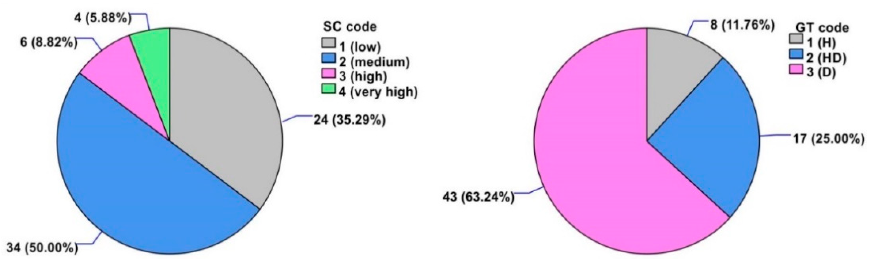
| Ordinal Variable (Factor) | Level of Factor | Code | Frequency | Relative Frequency |
|---|---|---|---|---|
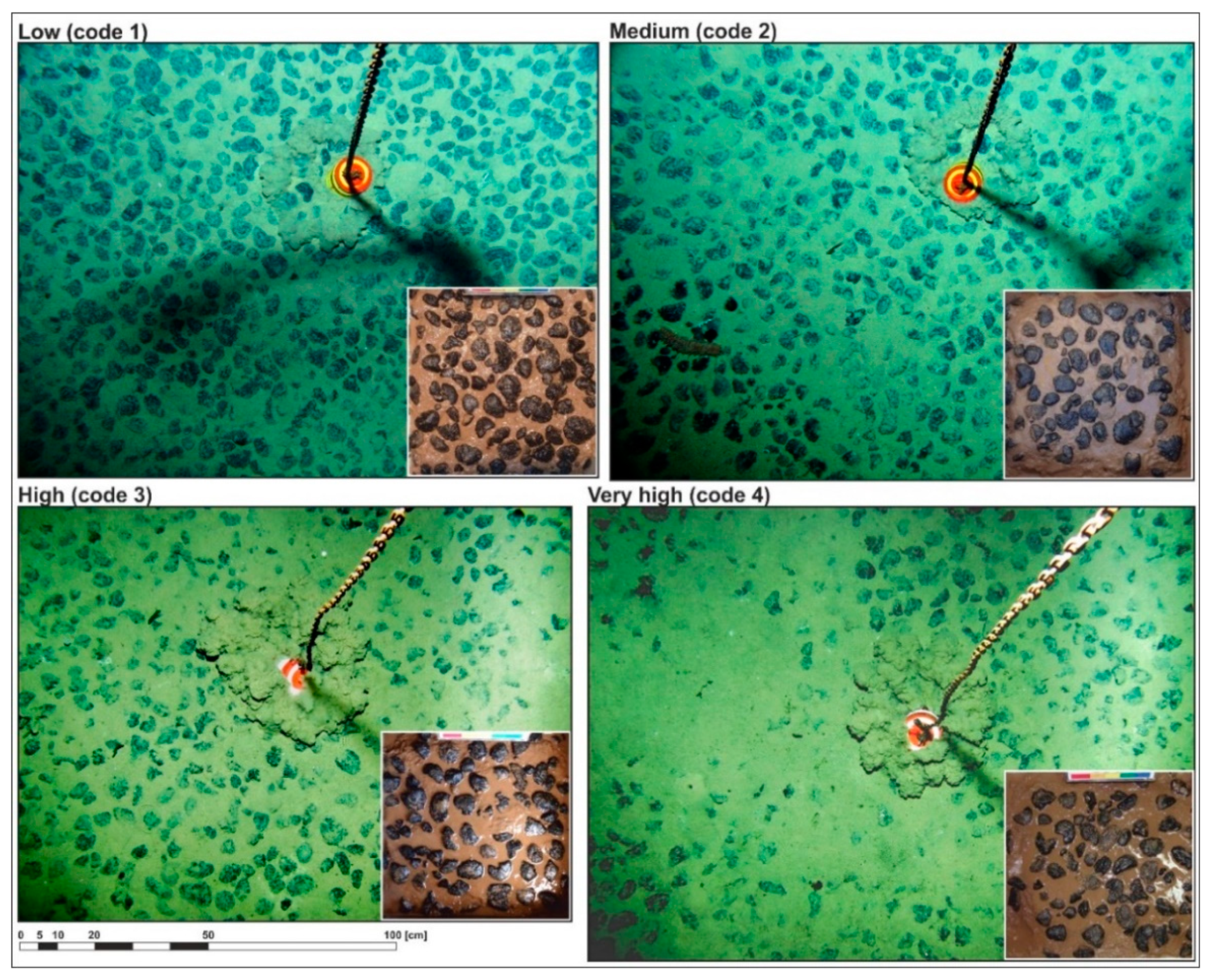
| Sediment coverage (SC) | Low | 1 | 24 | 35.3% |
| Medium | 2 | 34 | 50.0% | |
| High | 3 | 6 | 8.8% | |
| Very high | 4 | 4 | 5.9% | |
| Genetic type of nodules (GT) | H | 1 | 8 | 11.8% |
| HD | 2 | 17 | 25.0% | |
| D | 3 | 43 | 63.2% |
| Data Set (Count of Data = 68) | Regression Method | Independent Variables | Equation of Estimated Model | p-Value | SEE | MAE | MPE | MAPE |
|---|---|---|---|---|---|---|---|---|
| Grid photographs | SLM | NC-T | APN[kg/m2] = 1.33 + 0.27 NC-T[%] | 59.2 (0.0130) | 2.96 | 2.23 | −7.3 | 20.9 |
| ln(NC-T) | APN[kg/m2] = −14.17 + 7.38 ln(NC-T[%]) | 52.6 (0.0000) | 3.19 | 2.58 | −2.0 | 28.0 | ||
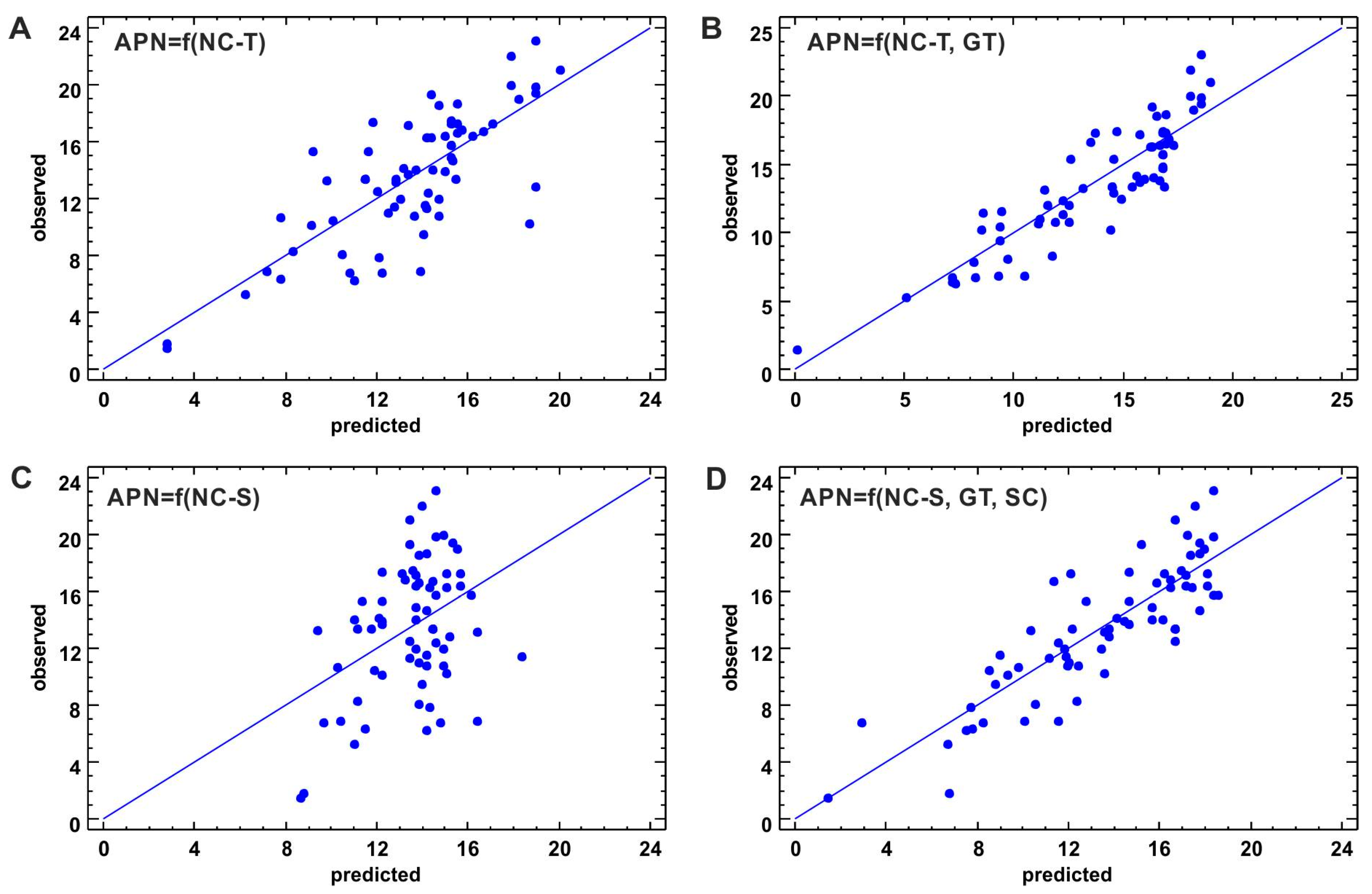
| GLM | NC-T, GT | APN[kg/m2] = 0.57 − 2.70I1(1) − 0.42I1(2) + 0.25NC-T[%] | 80.7 (0.0000) | 2.04 | 1.53 | −6.8 | 17.3 | |
| ln(NC-T), GT | APN[kg/m2] = −15.82 − 3.20I1(1) − 0.40I1(2) + 7.34ln(NC-T[%]) | 81.7 (0.0000) | 1.98 | 1.56 | 0.1 | 14.8 | ||
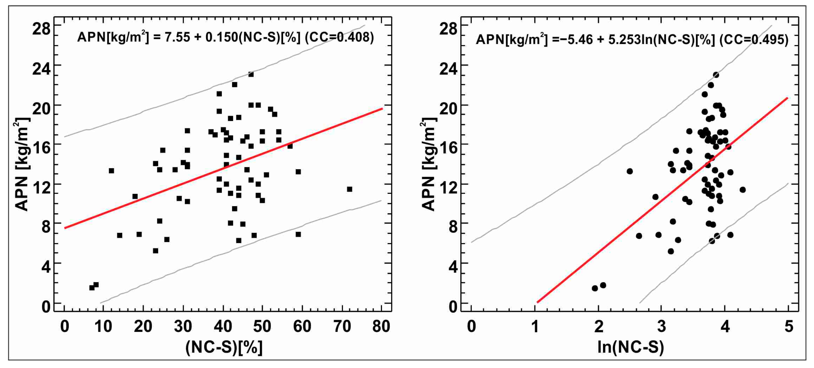
| Seafloor photographs | SLM | NC-S | APN[kg/m2] = 7.55 + 0.15 NC-S | 15.4 (0.0000) | 4.27 | 3.56 | −21.4 | 41.7 |
| ln(NC-S) | APN[kg/m2] = −5.46 + 5.25ln(NC-S[%]) | 23.3 (0.0000) | 4.06 | 3.39 | −15.5 | 34.9 | ||
| GLM | NC-S, GT | APN[kg/m2] = 2.65 − 4.16I2(1) − 0.48I2(2) + 0.22NC-S[%] | 60.2 (0.0000) | 2.92 | 2.26 | −14.6 | 29.8 | |
| NC-S, GT, SC | APN[kg/m2] = 0.95 − 1.73I1(1) − 0.01I1(2) + 0.02I1(3) − 4.30I2(1) − 0.46I2(2) + 0.27NC-S[%] | 61.0 (0.0000) | 2.90 | 2.14 | −13.6 | 28.0 | ||
| ln(NC-S), GT | APN[kg/m2] = −13.25 − 3.82I2(1) − 0.73I2(2) + 6.79ln(NC-S[%]) | 67.4 (0.0000) | 2.65 | 2.05 | −8.4 | 22.3 | ||
| ln(NC-S), GT, SC | APN[kg/m2] = −20.02 − 2.10I1(1) − 0.60I1(2) − 0.83I1(3) − 4.10I2(1) − 0.61I2(2) + 8.90ln(NC-S[%]) | 70.4 (0.0000) | 2.52 | 1.88 | −6.2 | 18.8 |
| Model | Parameter | Test Subset 1 | Test Subset 2 | Test Subset 3 |
|---|---|---|---|---|
| SLM Simple linear model APN = f(NC-S) | p-value | 0.0146 | 0.2182 | 0.0497 |
| 24.9% | 3.2% | 15.3% | ||
| MD | −0.23 (−1.7%) | 0.49 (3.8%) | −1.50 (−10.2%) | |
| MAD | 3.49 (25.6%) | 3.57 (27.2%) | 3.67 (25.1%) | |
| GLM General linear model APN = f(NCS, GT, SC) | p-value | 0.0000 | 0.0000 | 0.0009 |
| 68.0% | 65.7% | 43.7% | ||
| MD | 0.73 (5.4%) | 0.39 (3.0%) | −1.01 (−6.9%) | |
| MAD | 2.22 (16.3%) | 2.03 (15.5%) | 2.71 (18.5%) | |
| GLM(ln(NC-S)) General linear model with ln(NC-S) APN = f(ln(NC-S), GT, SC) | p-value | 0.0000 | 0.0000 | 0.000 |
| 77.9% | 65.9% | 59.6% | ||
| MD | 0.11 (0.8%) | 0.37 (2.8%) | −1.05 (−7.2%) | |
| MAD | 1.86 (13.6%) | 2.06 (15.7%) | 2.40 (16.4%) |
Publisher’s Note: MDPI stays neutral with regard to jurisdictional claims in published maps and institutional affiliations. |
© 2021 by the authors. Licensee MDPI, Basel, Switzerland. This article is an open access article distributed under the terms and conditions of the Creative Commons Attribution (CC BY) license (https://creativecommons.org/licenses/by/4.0/).
Share and Cite
Wasilewska-Błaszczyk, M.; Mucha, J. Application of General Linear Models (GLM) to Assess Nodule Abundance Based on a Photographic Survey (Case Study from IOM Area, Pacific Ocean). Minerals 2021, 11, 427. https://doi.org/10.3390/min11040427
Wasilewska-Błaszczyk M, Mucha J. Application of General Linear Models (GLM) to Assess Nodule Abundance Based on a Photographic Survey (Case Study from IOM Area, Pacific Ocean). Minerals. 2021; 11(4):427. https://doi.org/10.3390/min11040427
Chicago/Turabian StyleWasilewska-Błaszczyk, Monika, and Jacek Mucha. 2021. "Application of General Linear Models (GLM) to Assess Nodule Abundance Based on a Photographic Survey (Case Study from IOM Area, Pacific Ocean)" Minerals 11, no. 4: 427. https://doi.org/10.3390/min11040427