Article

Multidimensional Optimization of the Copper Flotation in a Jameson Cell by Means of Taxonomic Methods

1
Department of Environmental Engineering, Faculty of Mining and Geoengineering, AGH University of Science and Technology, al. Mickiewicza 30, 30-059 Kraków, Poland
2
JSW Innowacje S.A., ul. Paderewskiego 41, 40-282 Katowice, Poland
3
Faculty of Engineering, Kütahya Dumlupinar University, Evliya Çelebi Yerleşkesi Tavşanlı Yolu 10.km, 43100 Kütahya, Turkey
*
Author to whom correspondence should be addressed.
Minerals 2021, 11(4), 385; https://doi.org/10.3390/min11040385
Submission received: 16 February 2021 / Revised: 29 March 2021 / Accepted: 31 March 2021 / Published: 3 April 2021

Abstract

:
Three factors were measured in the flotation process of copper ore: the copper grade in a concentrate (β), the copper grade in tailings (ϑ), and the recovery of copper in a concentrate (ε). The experiment was conducted by means of a Jameson cell. The factors influencing the quality of the process were the particle size (d), the flotation time (t), the type of collector (k), and the dosage of the collector (s). The considered vector function is then (β(d, t, k, s), ϑ(d, t, k, s), ε(d, t, k, s)). In this work, the optimization was based on determining the values of the adjustable factors (d, t, k, s). The goal was to obtain the possibly highest values of the functions β and ε (maximum) with the possibly lowest values of the function ϑ (minimum). To this end, taxonomic methods were applied. Thanks to the applied method, the optimum—with the adopted assumptions—was found. The presented methodology can be successfully applied in the search for the optima in a variety of technological processes.

1. Introduction

The main operation of copper ore beneficiation, after its preparation in the processes of fragmentation and classification, consists in the application of the flotation process in the multi-stage final grinding and cleaning systems. Polish copper ore is characterized by three main lithological fractions which require a different way of beneficiation, with flotation as the second stage of the process. The main lithological fractions are presented in Table 1 showing the characteristics of the feed entering the technological system. The percentage shares of all lithological types vary depending on the region of occurrence. The content of copper in the ore used as feed for the process of beneficiation in processing plants changes depending on the lithological content of the feed, which is closely related to its region of occurrence. Therefore, the technology of copper ore beneficiation depends on its lithological composition. For this reason, the general ore processing variant cannot be used as its mineralogical and qualitative composition changes in the same way as mining and geological conditions of ore occurrence change. Apart from copper, the feed for beneficiation contains associated elements, i.e., silver, gold, platinum, and others, which also occur in varying amounts and are associated with the lithological type. The occurrence of three lithological types of Polish copper ore depostis significantly hinders the process of output beneficiation due to the diversity of their mineralogical and physico-chemical properties. The decrease in the size of ore-bearing particles observed in recent years makes it necessary to perform the grinding in finer size particle distributions with the aim to release copper-bearing particles. However, flotation of very fine particles is difficult to perform in efficient way [1]. Therefore, it is necessary to use a new generation of machines with adequately selected bubble size distribution, which enable the adhesion of extremely fine particles [2]. In general, the processing of ore and the production of a concentrate for metallurgical processes of suitable quality requires that the process of beneficiation is conducted with utmost care in order to ensure optimal quantitative and qualitative parameters of the produced feed for metallurgy [1]. From the perspective of the assessment of the processing plant’s final product, the most important assessment indicators comprise the content of copper in the concentrate, the waste, as well as the yield of copper in the concentrate. The process of mineral flotation depends on many factors, i.e., the minerals’ nature and structure (mineralogy, morphology, and particle size), water chemistry, bubble size and velocity, flotation time, hydrodynamic properties, pulp potential and pH, pulp density, air flow rate, as well as reagent types and dosages [1,2,3,4,5]. To achieve the best possible indicators, the process of flotation is conducted with the optimization of some technical and technological parameters.
Many studies on ore flotation are available in the literature. Most of them deal with various optimization issues. With regard to copper ores, many papers discuss the problem of selecting appropriate reagents and their dosages. The use and selection of new kinds of reagents for the process was the topic of the studies presented in [7,8,9,10,11]. The introduction of seawater was presented in [12]. The effect of desliming on flotation efficiency was investigated by [13]. Podariu et al. discussed the role of metallic electrodes in the process [14]. The problem of bubble size distribution as well air rate and froth depth were the object of interest in [2,15]. The application of ultrasound at various stages of the copper flotation process was discussed in [16]. One of the main factors for evaluating the quality of the process is the selectivity index. A study on the impact of the process parameter modification was presented in [17,18]. The surface oxidation level was investigated in [19]. Furthermore, various attempts in the modeling of the whole process or parts of it, introducing different types of algorithms, were presented in many papers [20,21,22,23,24,25,26]. We have also conducted many studies on copper ore processing and its optimization. Many different methods were applied for this purpose. A parametric optimization in mixed copper ores flotation was presented in [27]. A geometrical approach was the subject presented in [28]. A combined approach consisting of neural networks and evolutionary algorithms was shown in [29]. Non-classical statistical methods, such as kernel methods, Fourier series method, or non-parametric statistical methods were introduced in [30]. Applications of ANOVA (Analysis of Variance) in mineral processing, including also copper flotation were discussed in [31]. The initial studies of the copper flotation process conducted in a Jameson cell was the subject presented in [32]. To this end, we used taxonomic methods, which are an innovative approach to optimize the process. Copper grade in concentrate (β), copper grade in tailings (ϑ), and copper recovery in a concentrate (ε) were selected as factors for the evaluation of the flotation performance (performance indicators). In this study, adjustable factors that influence flotation quality are the particle size (d), the separation time (t), the collector type (k), and the collector dosage (s).

2. Experiment

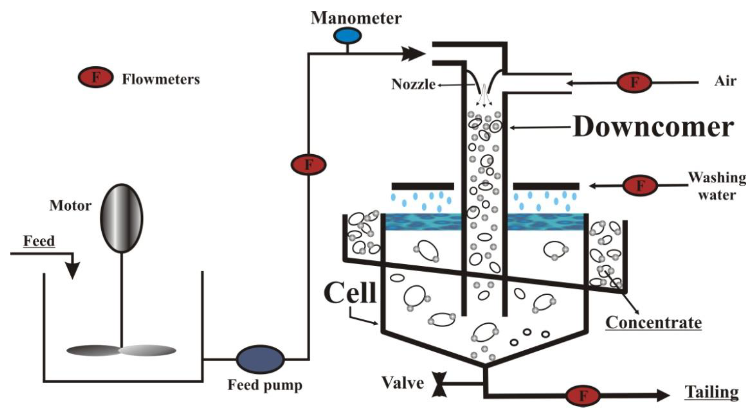
2.1. Laboratory Investigation

The experimental research was conducted through a Jameson cell. It is a pneumatic flotation device in which pressurized, naturally aspirated air is dispersed. It is responsible for the mixing of the suspension. The device consists of two main parts, which are the downcomer and the separation tank. Conditioned particles are pumped to the nozzle at the top of the downcomer to create a high-pressure water jet, and the air is sucked into the downcomer. This water jet is responsible for producing a high-intensity mixing and fine bubbles. Thus, the downcomer becomes the first contact point of particles and air bubbles. Micro-events of flotation occur in the downcomer, and hydrophobic particles become attached to air bubbles. A bubbly mixture is discharged to the separation tank from the downcomer. The separation tank provides a suitable environment for the separation of hydrophilic particles from the particle-laden bubbles. Hydrophobic particles–bubbles aggregates are raised to the froth zone. There is a water washing system, which positively impacts the selectivity of the process [33,34,35,36,37,38].
During this operation, fine bubbles increase the collision between bubbles and particles and improve the flotation kinetics. This characteristic lowers the requirements regarding particle retention time and makes it possible to decrease the Jameson cell height compared to traditional flotation columns [39,40,41,42].
The investigated material was Polish carbonate copper ore. The initial copper grade in the feed equaled 1.5%. From the lithological point of view, it contained minerals, such as carbonates (dolomite, calcite)—about 72%, shale minerals—about 16%, sulfates (gypsum, anhydrite)—5%, quartz—3%, copper sulfides—3% and organic substance—0.5%. The Jameson cell scheme is presented in Figure 1.
The parameters of the flotation machine were the following:
  • separation tank diameter and height 200 mm and 900 mm, respectively;
  • downcomer diameter and length: 0.020 m and 1.8 m, respectively;
  • nozzle diameter 0.005 m;
  • conditioning tank volume: 0.1 m3;
  • downcomer plunging length that is the depth to which the end of the downcomer is immersed in the separation tank: 0.5 m;
  • feed rate and air rate: 100 cm3/s.
The investigation was based on the changes in the course of the process, caused by the changes in the individual factors (adjustable variables). Particle fractions −20, 20–40, and 40–71 μm were prepared for the tests. For each level of the experiment, it was necessary to repeat the process in order to verify the adequacy of the results. The results of the laboratory experiments were significant and the values of errors did not exceed the acceptable limits (<5%) which were evaluated using the standard deviation. It was assumed that the maximum time of flotation would amount to 30 min. The concentrate was collected selectively after 1, 2, 4, 6, 9, 12, 17, 22, and 30 min. As a result, it was possible to analyze the kinetics of the separation as well as the influence of time on the effects of beneficiation. The solids grade in the Jameson cell was maintained at a constant level of 2%. The Nasfroth frother was added to the amount of 50 g/t. The final stage was to determine the copper content in the separation products with the use of the XRF methodology, which made it possible to calculate process factors, such as the copper grade in the concentrate β, the copper grade in the tailings ϑ, and the copper recovery in the concentrate ε.
The variables were selected on the basis of previous experiments which showed that these factors are strongly related to the efficiency of the flotation process [34,35]. The values of these adjustable factors are outlined in Table 2.
For each determined value of the adjustable parameters (d, t, k, s) five measurements of researched flotation factors were performed, which results in a vector (β, ϑ, ε).
The averaged results of measurements and calculations are presented in Table 3, Table 4 and Table 5.
Table 3 presents the results experimentally obtained for the particle size fraction −20 µm for both reagent types (E, I) at doses of 100 and 150 (g/t), depending on the flotation time.
Table 4 shows analogous results, but for the fraction 20-40 µm. Similarly, as in the case of the finest size fraction, it is also difficult to determine the optimal point of the process in this case, taking into consideration the values of all three technological indicators.
Table 5 shows the results obtained for the fraction 40–71 µm. The conclusions are similar. Multivariate statistical methods must be used in order to determine the optimal conditions. This paper proposes the application of taxonomic methods, whose use is innovative in the context of problems related to the the processing of raw materials.

2.2. Methodology of Taxonomic Methods

2.2.1. Theoretical Background

The selected taxonomical methods found wide application in various scientific disciplines [43,44,45,46], because their major advantages are universality, simplicity of calculations, and simple interpretation of the results. The taxonomic factors allow to replace the description of the considered multi-feature object by means of one synthetic variable. The complex structure of the flotation process as well as the changeability of the investigated copper ore make it necessary to apply multidimensional methods for data analysis [47,48,49,50]. The basis to conduct the multidimensional comparison analysis is a matrix of diagnostic features X (1), which is then standardized and transformed into a synthetical factor Z (2). All considered situations are put in order in a linear way with consideration of the positive influence (stimulants) and the negative influence (destimulants) on the researched phenomenon. Then the surrogate variable is introduced as the distance between the objects which allow to evaluate the phenomenon. The development of the taxonomy caused the introduction of various factors and methods of variable normalization [51].
X = [ x 11 x 12 x 1 l x 21 x 22 x 2 l x n 1 x n 2 x nl ]
Z = [ z 11 z 12 z 1 l z 21 z 22 z 2 l z n 1 z n 2 z nl ]
Among the taxonomical methods many factors can be used. In this work, the Euclidean distance ej was used, whose general formula is presented by Equation (3).
e i = j = 1 l ( 1 z ij ) 2   for   i = 1 , ,   n .
where:
  • i—number of the row;
  • j—number of the column;
  • n—number of investigated variables (flotation tests);
  • l—number of variables (process evaluation factors);
    z ij = x ij x jmax ,   x jmax = max i ( x ij ) standardized   value .
For such determined values of zij the values e1, e2, …, en were calculated by means of Equation (3). The smallest value allowed us to determine the optimal values of the considered factors.
The precise description of how to conduct the investigation by means of taxonomic methods can be found in [45,47,51].

2.2.2. Application

The multidimensional projection considered in this work takes the following form:
f : ( d , t , k , s ) ( β ( d , t , k , s ) , ϑ ( d , t , k , s ) , ε ( d , t , k , s ) )
where values of variables (d, t, k, s) are accepted in accordance with the values proposed in Table 2.
Next, the optimization of the flotation process is performed. It is based on the determination of such values of adjustable factors (d, t, k, s) for which the functions β and ε assume simultaneously the biggest values and the function ϑ the smallest one.
Because of the fact that it is required that the variables β and ε reach the highest possible values in order to be qualified as flotation process stimulants, while the variable ϑ is treated as a destimulant. According to the taxonomic methods, destimulants should be transferred to become stimulants. That is why a new variable, 1 ϑ i , is introduced instead of the variable ϑ.
In order to enable the comparison of various values, they need to be normalized first. It can be done by the introduction of new variables, according to Equations (6)–(8).
ε i ˜ = ε i max j ε j
β i ˜ = β i max j β j
ϑ i ˜ = 1 ϑ i max j 1 ϑ j
Selection of the optimal adjustable variables is performed using the function of minimization
F ( β ( d , t , k , s ) , ϑ ( d , t , k , s ) , ε ( d , t , k , s ) )
where
F ( β i , ϑ i , ε i ) = ( 1 ε i ˜ ) 2 + ( 1 β i ˜ ) 2 + ( 1 ϑ i ˜ ) 2
where ε i ˜ , β i ˜ , ϑ i ˜ are provided by Equations (6)–(8).

3. Results and Discussion

The optimization of the function F was carried out with the use of the determined particle size fractions, the type of collector and its dosage. At the second stage, the optimal values were obtained with the use of the determined particle size fraction and the type of collector; finally, it was carried out only with the use of the assumed particle size fraction. The obtained results are shown in Table 6, Table 7 and Table 8.
Table 6 shows the calculated indices of optimal values for the sought indices β, ϑ and ε for the assumed particle fractions, the collector type and the dosage. The analysis of the obtained results made it possible to observe that the best quality concentrate, with a copper content amounting to 11.9% for the type 1 collector in the amount of 100 g/t, for the finest particle fraction, within 22 min, was obtained for the finest particle fraction −20 μm. Satisfactory copper recovery in an 88.2% concentrate and copper content in tailings of 0.5% were also obtained in these conditions of the flotation process. For particles of an average size, floating in the Jameson cell 20–40 μm, the taxonomic analysis showed that at a lower dosage of both types of reagents, comparable results −7.1% and 6.3%, respectively, were obtained with regard to β. On the other hand, much better optimal conditions of recovery ε = 67.7% and copper content in tailings ϑ = 0.1% were obtained for type E reagents in the first three minutes of flotation. Together with an increase in the dosage of type I reagent to 150 g/t, the recovery increases to approx. 70%, but has a negative impact on β and ϑ. In the case of the coarsest floating particle fraction 40–71 μm, the optimal β, ϑ, and ε indices, calculated according to the presented method, in each case reached the lowest values.
Table 7 shows the calculated indices of optimal values for the searched β, ϑ, and ε indices, for the assumed particle fractions and collector types. It is worth noting that with the use of the type 1 collector for the finest particle fraction, better optimal results are obtained with a higher dosage within the same time. Similarly, in the case of a medium size fraction, higher optimal indices were obtained for a higher collector dosage 150 g/t of type 1, β = 10.5%, ϑ = 0.9%, and ε = 70.9% within less than 12 min. For the coarse particle fraction, the optimal β, ϑ, and ε values were obtained for the type E collector, 100 g/t of dosage, but within a longer time.
Table 8 shows indices of optimal values for the sought β, ϑ, and ε indices for the assumed particle fractions. The best optimum rates were obtained for the finest particle fraction with the use of the type I collector, a dosage of 100g/t and during a 22-min flotation.
The next stage was to perform the optimization within the assumed time. The results of this stage are presented in Table 9. If we take into account the flotation type, the best optimum rates were obtained for the finest particle size fraction −20 μm. In this case, the highest β value was determined at the level of 17.5% after 4 min of flotation time. The highest values of the indicators, ϑ = 0.4% and ε = 89.5%, were obtained after 30 min of flotation. Hence, the conclusion is that the longer the time of flotation, the higher is the recovery and the lower the copper content in the waste in the given process conditions for the finest particles.
The relations between the optimal values of β, ϑ, ε, and time t are presented in Figure 2, Figure 3 and Figure 4.
The last stage concerned the optimization in a set of considered values of adjustable variables (Table 2) and the solution is presented in Table 10. Therefore, the optimum conditions of the process were found.
On the basis of the results, it can be said that the best particle size fraction for the process is 0–20 µm with Aqueous solution of isobutyl sodium xanthate in a dosage of 100 g/t. The optimal time of flotation is 22 min. Therefore, the optimal value of the function F is equal to 0.376; it is related to the values of β, ϑ, and ε as 11.9%, 0.5%, and 88.2%, respectively.
The Jameson cell has problematic behavior in coarse particle flotation. Sahbaz et al. [40] proved that the maximum size of floating particles having different hydrophobicity degree in various hydrodynamic regions can differ. The results presented in this paper were based on the flotation tests performed in a Jameson cell of the same geometrical properties as was used in [40]. Experiments and literature findings indicate that the turbulence is the most significant parameter in the coarse particle flotation. The stability of the aggregate starts to decrease as the particle size increases, meaning that the detachment force starts to overwhelm the attachment force [38,52,53,54]. Furthermore, the finer fraction accumulates the biggest amount of copper. This is the reason why this particle size fraction has the biggest potential of copper particle recovery in special conditions. The Jameson cell serves best for this purpose because of its construction and characteristic air bubbles size distribution [55]. The Jameson cell has significant potential to separate fine particle due to very fine bubble production [56,57]. In this test, the results for fine particles are quite good due to these characteristics. In addition, the liberation degree of the sample is higher for the finer size fraction [58]. A conventional cell shows problematic flotation for finer particles due to coarse bubble size causing low collision probability [37,38].

4. Conclusions

The methodology of the optimization of copper flotation results, consisting in the use of the taxonomic method with regard to the beneficiation in a Jameson cell made it possible to determine the optimal conditions of its operation, depending on variable factors, namely the size of particles, the type and dosage of reagent, flotation type for the evaluation indicators of key processes, commonly used in raw material processing. Analyzing the obtained results, it can be observed that for almost all values of time (except t = 1 min and t = 2 min) the best type of the collector was an Aqueous solution of isobutyl sodium xanthate. It is worth noticing that the best dosage of the collector for the time t ≥ 4 (min) was a dosage of 100 g/t, while for the time t < 4 min it was a dosage of 150 g/t. For smaller particle size fractions (0–20 and 20–40 µm), the Aqueous solution of isobutyl sodium xanthate was a better type of collector, while for the bigger one (40–71 µm) it was xanthate. Analyzing the process depending on particle size, it can be noticed that the best results were obtained definitely for the particle size fraction 0–20. The optimal time in individual cases varied from 12 min to 30 min, but the most suitable time was 22 min. In addition, if the considered indicators are differed in terms of their relevance (if, for example, the economic factors were taken into account), appropriate weights, w1, w2, w3, can be entered into the optimization function. In such a case, particular components of the F function should be multiplied by w1, w2, w3, respectively, where 0 < w1 < 1, 0 < w2 < 1, 0 < w3 < 1 and w1 + w2 + w3 = 1. The presented methodology can be used efficiently in the evaluation of all kinds of processes and when combined with modeling methods, it can be used as an algorithm of process quality monitoring.

Author Contributions

Conceptualization; methodology; data curation; writing—original draft preparation, T.N.; formal analysis; investigation; writing—original draft, P.P.; writing—review and editing; supervision; validation, A.S., O.Ş. All authors have read and agreed to the published version of the manuscript.

Funding

This research received no external funding.

Acknowledgments

The paper is a result of project no. 11.11.100.276.

Conflicts of Interest

The authors declare no conflict of interest.

References

  1. Bulatovic, S.M. Handbook of Flotation Reagents Chemistry, Theory and Practice: Flotation of Sulfide Ores; Elsevier Science & Technology: Amsterdam, The Netherlands, 2007. [Google Scholar]
  2. Wang, L.; Xing, Y.; Wang, J. Mechanism of the combined effects of air rate and froth depth on entrainment factor in copper flotation. Physicochem. Probl. Miner. Process. 2020, 56, 43–53. [Google Scholar]
  3. Rahman, R.M.; Ata, S.; Jameson, G.J. The effect of flotation variables on the recovery of different particle size fractions in the froth and the pulp. Int. J. Miner. Process. 2012, 106, 70–77. [Google Scholar] [CrossRef]
  4. Hassanzadeh, A.; Hassas, B.V.; Kouachi, S.; Brabcova, Z.; Çelik, M.S. Effect of bubble size and velocity in chalcopyrite flotation. Colloids Surf. A 2016, 498, 258–267. [Google Scholar] [CrossRef]
  5. Ucurum, M.; Bayat, O. Effects of operating variables on modified flotation parameters in the mineral separation. Sep. Purif. Technol. 2007, 55, 173–181. [Google Scholar] [CrossRef]
  6. Piestrzyński, A. Monograph KGHM Polska Miedź S.A.; Part 2, Geology, 2.19. Litology; CBPM Cuprum: Lubin, Poland, 1996. [Google Scholar]
  7. Dhar, P.; Thornhill, M.; Rao Kota, H. Investigation of Copper Recovery from a New Copper Ore Deposit (Nussir) in Northern Norway: Dithiophosphates and Xanthate-Dithiophosphate Blend as Collectors. Minerals 2019, 9, 146. [Google Scholar] [CrossRef] [Green Version]
  8. Dhar, P.; Thornhill, M.; Rao Kota, H. Investigation of Copper Recovery from a New Copper Deposit (Nussir) in Northern-Norway: Thionocarbamates and Xanthate-Thionocarbamate Blend as Collectors. Minerals 2019, 9, 118. [Google Scholar] [CrossRef] [Green Version]
  9. Filip, G.; Podariu, M. Advanced Recovery of Complex Ores using Emulsions of Non-polar Reagents. Sci. Bull. Ser. D 2010, 24, 53–56. [Google Scholar]
  10. Zhu, R.; Gu, G.; Chen, Z.; Wang, Y.; Song, S. A New Collector for Effectively Increasing Recovery in Copper Oxide Ore-Staged Flotation. Minerals 2019, 9, 595. [Google Scholar] [CrossRef] [Green Version]
  11. Ziyadanogullari, R.; Aydin, F. A New Application For Flotation Of Oxidized Copper Ore. J. Miner. Mater. Charact. Eng. 2005, 4, 67–73. [Google Scholar] [CrossRef]
  12. Gutierrez, L.; Betancourt, F.; Uribe, L.; Maldonado, M. Influence of Seawater on the Degree of Entrainment in the Flotation of a Synthetic Copper Ore. Minerals 2020, 10, 615. [Google Scholar] [CrossRef]
  13. Phiri, T.; Tepa, C.; Nyati, R. Effect of Desliming on Flotation Response of Kansanshi Mixed Copper Ore. J. Miner. Mater. Charact. Eng. 2019, 7, 193–212. [Google Scholar] [CrossRef] [Green Version]
  14. Podariu, M.; Ilie, P.; Filip, G. Role of Metallic Electrodes in Flotation Activation Phenomena. Sci. Bull. Ser. D 2009, 23, 121–124. [Google Scholar]
  15. Han, Y.; Zhu, J.; Shen, L.; Zhou, W.; Ling, Y.; Yang, X.; Wang, S.; Dong, Q. Bubble Size Distribution Characteristics of a Jet-Stirring Coupling Flotation Device. Minerals 2019, 9, 369. [Google Scholar] [CrossRef] [Green Version]
  16. Hassanzadeh, A.; Sajjady, S.A.; Gholami, H.; Amini, S.; Özkan, S.G. An Improvement on Selective Separation by Applying Ultrasound to Rougher and Re-Cleaner Stages of Copper Flotation. Minerals 2020, 10, 619. [Google Scholar] [CrossRef]
  17. Azizi, A. A study on the modified flotation parameters and selectivity index in copper flotation. Part. Sci. Technol. 2017, 35, 38–44. [Google Scholar] [CrossRef]
  18. Azizi, A. Optimization of rougher flotation parameters of the Sarcheshmeh copper ore using a statistical technique. J. Dispers. Sci. Technol. 2015, 36, 1066–1072. [Google Scholar] [CrossRef]
  19. Moimane, T.; Plackowski, C.; Peng, Y. The critical degree of mineral surface oxidation in copper sulphide flotation. Miner. Eng. 2020, 145, 106075. [Google Scholar] [CrossRef]
  20. Matsuoka, H.; Mitsuhashi, K.; Kawata, M.; Tokoro, C. Derivation of Flotation Kinetic Model for Activated and Depressed Copper Sulfide Minerals. Minerals 2020, 10, 1027. [Google Scholar] [CrossRef]
  21. Wang, S.; Li, Y.; Zhai, X.; Guan, W. A Recognition Method based on Improved Watershed Segmentation Algorithm or Copper Flotation Conditions. In Proceedings of the 2019 Chinese Automation Congress (CAC), Hangzhou, China, 22–24 November 2019; pp. 224–231. [Google Scholar]
  22. Wang, Z.; He, D.; Li, B. Clustering of Copper Flotation Process Based on the AP-GMM Algorithm. IEEE Access 2019, 7, 160650–160659. [Google Scholar] [CrossRef]
  23. Ghodrati, S.; Nakhaei, F.; VandGhorbany, O.; Hekmati, M. Modeling and optimization of chemical reagents to improve copper flotation performance using response surface methodology. Energy Sour. Part A 2020, 42, 1633–1648. [Google Scholar] [CrossRef]
  24. Bahrami, A.; Ghorbani, Y.; Hosseini, M.R.; Kazemi, F.; Abdollahi, M.; Danesh, A. Combined Effect of Operating Parameters on Separation Efficiency and Kinetics of Copper Flotation. Min. Metall. Explor. 2019, 36, 409–421. [Google Scholar] [CrossRef] [Green Version]
  25. Hassanzadeh, A.; Firouzi, M.; Albijanic, B.; Celik, M.S. A view on determination of particle–bubble encounter using analytical, experimental and numerical methods. Miner. Eng. 2018, 122, 296–311. [Google Scholar] [CrossRef]
  26. Saramak, D.; Tumidajski, T.; Skorupska, B. Technological and economic strategies for the optimization of Polish electrolytic copper production plants. Miner. Eng. 2010, 23, 757–764. [Google Scholar] [CrossRef]
  27. Azizi, A.; Masdarian, M.; Hassanzadeh, A.; Bahri, Z.; Niedoba, T.; Surowiak, A. Parametric optimization in rougher flotation performance of a sulfidized mixed copper ore. Minerals 2020, 10, 660. [Google Scholar] [CrossRef]
  28. Foszcz, D.; Niedoba, T.; Tumidajski, T. A geometric approach to evaluating the results of Polish copper ores beneficiation. Gospod. Surowcami Min. 2018, 34, 55–66. [Google Scholar]
  29. Jamróz, D.; Niedoba, T.; Pięta, P.; Surowiak, A. The use of neural networks in combination with evolutionary algorithms to optimise the copper flotation enrichment process. Appl. Sci. 2020, 10, 3119. [Google Scholar] [CrossRef]
  30. Niedoba, T. Determination of partition surface of grained material by means of non-classical approximation methods of distributions functions of particle size and density. Gospod. Surowcami Min. 2016, 32, 137–154. [Google Scholar] [CrossRef] [Green Version]
  31. Niedoba, T.; Pięta, P. Applications of ANOVA in mineral processing. Min. Sci. 2016, 23, 43–54. [Google Scholar]
  32. Pięta, P.; Niedoba, T.; Surowiak, A.; Şahbaz, O.; Karagüzel, C.; Canieren, Ö. Studies on Polish copper ore beneficiation in Jameson cell. In IOP Conference Series: Materials Science and Engineering; IOP Publishing: Bristol, UK, 2018; Volume 427, p. 012009. [Google Scholar]
  33. Evans, G.M.; Atkinson, B.W.; Jameson, G.J. The Jameson Cell. Flotat. Sci. Eng. 1995, 11, 331–363. [Google Scholar]
  34. Harbort, G.; Manlapig, E.V.; Debono, S. A discussion of particle collection within the Jameson Cell downcomer. T. I. Min. Metall. C 2002, 307, C1–C10. [Google Scholar]
  35. Harbort, G.; Debono, S.; Carr, D.; Lawson, V. Jameson Cell Fundamentals—A revised perspective. Miner. Eng. 2003, 16, 1091–1101. [Google Scholar] [CrossRef]
  36. Mohanty, M.K.; Honaker, R.Q. Performance optimization of Jameson flotation technology for fine coal cleaning. Miner. Eng. 1999, 12, 367–381. [Google Scholar] [CrossRef]
  37. Gontijo, F.C.; Fornasiero, D.; Ralston, J. The limits of fine and coarse particle flotation. Can. J. Chem. Eng. 2017, 85, 739–747. [Google Scholar] [CrossRef]
  38. Kowalczuk, P.B.; Şahbaz, O.; Drzymała, J. Maximum size of floating particles in different flotation cells. Miner. Eng. 2011, 24, 766–771. [Google Scholar] [CrossRef]
  39. Şahbaz, O.; Oteyaka, B.; Kelebek, Ş.; Uçar, A.; Demir, U. Separation of unburned carbonaceous matter in bottom ash using Jameson cell. Sep. Purif. Technol. 2008, 62, 103–109. [Google Scholar] [CrossRef]
  40. Şahbaz, O.; Uçar, A.; Oteyaka, B. Velocity gradient and maximum floatable particle size in the Jameson cell. Miner. Eng. 2013, 41, 79–85. [Google Scholar] [CrossRef]
  41. Foszcz, D. Rules of Determining the Optimal Results of Multi-Component Copper Ores Beneficiation; IGSMiE PAN: Kraków, Poland, 2013. [Google Scholar]
  42. Wieniewski, A.; Skorupska, B. Technology of Polish copper ore beneficiation—Perspectives from the past experience. In E3S Web of Conferences; EDP Sciences: Les Ulis, France, 2016; Volume 8, p. 01064. [Google Scholar]
  43. Aldrich, C. Cluster analysis of mineral process data with autoassociative neural networks. Chem. Eng. Commun. 2000, 177, 121–137. [Google Scholar] [CrossRef]
  44. Ginsberg, D.W.; Whiten, W.J. The application of clustering to the calibration of onstream analysis equipment. Int. J. Miner. Process. 1992, 36, 63–79. [Google Scholar] [CrossRef]
  45. Laine, S.; Lappalainen, H.; Jämsä-Jounela, S.L. One-line determination of ore type cluster analysis and neural networks. Miner. Eng. 1995, 6, 637–648. [Google Scholar] [CrossRef]
  46. Whiteley, J.R.; Davis, J.F. A similarity-based approach to interpretation of sensor data using adaptive resonance theory. Comput. Chem. Eng. 1994, 18, 637–661. [Google Scholar] [CrossRef]
  47. Ginsberg, D.W.; Whiten, W.J. Cluster analysis for mineral processing applications. T. I. Min. Metall. C 1991, 100, 139–146. [Google Scholar]
  48. Niedoba, T. Methodological elements of applying two—And multidimensional distributions of grained materials properties to coal beneficiation. Gospod. Surowcami Min. 2013, 29, 155–172. [Google Scholar] [CrossRef] [Green Version]
  49. Tumidajski, T. Actual tendencies in description and mathematical modeling of mineral processing. Gospod. Surowcami Min. 2010, 26, 111–123. [Google Scholar]
  50. Nakhaei, F.; Irannajad, M.; Sam, A.; Jamalzadeh, A. Application of d-optimal design for optimizing copper-molybdenum sulphides flotation. Physicochem. Probl. Miner. Process. 2015, 52, 252–267. [Google Scholar]
  51. Łuniewska, M.; Tarczyński, W. Methods of Multidimensional Comparative Analysis on the Capital Market; PWN: Warszawa, Poland, 2006. [Google Scholar]
  52. Drzymała, J. Characterization of materials by Hallimonf tube flotation. Int. J. Miner. Process. 1994, 42, 139–152. [Google Scholar] [CrossRef]
  53. Schulze, H.J. Dimensionless number and approximate calculation of the upper particle size of floatability in flotation machines. Int. J. Miner. Process. 1982, 9, 321–328. [Google Scholar] [CrossRef]
  54. Trahar, W.J. A rational interpretation of the role of particle size in flotation. Int. J. Miner. Process. 1981, 8, 289–327. [Google Scholar] [CrossRef]
  55. Evans, G.M.; Atkinson, B.; Jameson, G.J. The Jameson cell. In Flotation Science and Engineering. Marcel Dekker; Matis, K.A., Ed.; Wiley Online Library: Hoboken, NJ, USA, 1995; pp. 331–363. [Google Scholar]
  56. Jameson, G.J. New directions in flotation machine design. Miner. Eng. 2010, 23, 835–842. [Google Scholar] [CrossRef]
  57. Jameson, G.J.; Goel, S. New approaches to particle attachment and detachment in flotation. In Separation Technologies for Minerals, Coal, and Earth Resources; Society for Mining, Metallurgy, and Exploration; Young, C.A., Luttrell, G.H., Eds.; SME: Englewood, CO, USA, 2012; pp. 437–447. [Google Scholar]
  58. Jameson, G.J. The effect of surface liberation and particle size on flotation rate constants. Miner. Eng. 2012, 36–38, 132–137. [Google Scholar] [CrossRef]
Figure 1. Scheme of a Jameson cell [39].
Minerals 11 00385 g001
Figure 2. Relation βopt(t).
Minerals 11 00385 g002
Figure 3. Relation ϑopt(t).
Minerals 11 00385 g003
Figure 4. Relation εopt(t).
Minerals 11 00385 g004
Table 1. Mineralogical composition of lithological types of Polish copper ores [6].
Lithological Type of Copper OreContent of Selected Metals in Lithological TypesPrevalent Copper-Bearing Minerals
carbonatesCu (%)1.69chalcocite in combination with digenite, bornite, covellite and chalcopyrite
Ag (g/t)54
shalesCu (%)6.02chalcocite-bornite and bornite-chalcopyrite minerals
Ag (g/t)188
sandstonesCu (%)1.29bornite-chalcopyrite and chalcocite-bornite minerals
Ag (g/t)30
Table 2. Characteristics of adjustable factors.
Particle Size Fraction d (μm)Collector Type kCollector Dosage s (g/t)Time t (min)
0–20
20–40
40–71
Aqueous solution of ethyl sodium xanthate—E
Aqueous solution of isobutyl sodium xanthate—I
100
150
1, 2, 4
6, 9, 12
17, 22, 30
Table 3. Results of measurements for particle size fraction 0–20 (µm).
Time t (min)EI
100 (g/t)150 (g/t)100 (g/t)150 (g/t)
βϑεβϑεβϑεβϑε
10.1450.0240.0680.1130.0180.1520.1660.0260.1520.1710.0230.122
20.1710.0170.3560.1210.0130.4020.1840.0190.4160.1570.0180.359
40.1600.0120.5720.1130.0100.5940.1750.0130.6130.1500.0140.562
60.1410.0080.7090.1020.0070.7060.1560.0090.7370.1370.0090.706
90.1260.0060.7820.0920.0060.7720.1420.0070.8110.1240.0070.785
120.1150.0060.8020.0860.0050.7980.1310.0060.8330.1150.0060.809
170.1080.0050.8320.0810.0040.8300.1230.0060.8560.1070.0050.835
220.1040.0050.8580.0770.0040.8390.1190.0050.8820.1030.0050.856
300.0970.0040.8760.0720.0040.8560.1120.0040.8950.0970.0040.870
Table 4. Results of measurements for particle size fraction 20–40 (µm).
Time t (min)EI
100 (g/t)150 (g/t)100 (g/t)150 (g/t)
βϑεβϑεβϑεβϑε
10.0760.0240.0650.0650.0260.0170.0630.0180.0490.1670.0210.137
20.0760.0210.1880.0810.0230.1480.0750.0160.2200.1350.0130.336
40.0770.0190.3010.0780.0210.2560.0820.0130.4030.1210.0130.505
60.0750.0170.4140.0790.0190.3720.0740.0110.5090.1140.0100.633
90.0760.0150.5060.0770.0170.4530.0680.0100.5690.1050.0090.706
120.0730.0140.5450.0760.0160.5010.0630.0100.5890.0970.0080.733
170.0730.0120.6020.0730.0150.5380.0590.0090.6150.0910.0080.754
220.0740.0110.6450.0730.0140.5770.0580.0090.6390.0880.0070.777
300.0710.0110.6770.0710.0130.6100.0550.0090.6580.0830.0070.796
Table 5. Results of measurements for particle size fraction 40–71 µm.
Time t (min)EI
100 (g/t)150 (g/t)100 (g/t)150 (g/t)
βϑεβϑεβϑεβϑε
10.0750.0190.0320.0640.0200.0650.0920.0240.0240.0750.0250.041
20.0570.0170.1420.0650.0180.1930.0680.0220.1320.0680.0230.144
40.0570.0160.2530.0680.0160.3260.0680.0200.2380.0630.0220.226
60.0570.0140.3720.0720.0130.4670.0650.0190.3280.0600.0210.299
90.0580.0130.4620.0690.0110.5480.0620.0180.3860.0560.0200.348
120.0580.0120.5150.0670.0100.5920.0590.0170.4130.0550.0200.382
170.0560.0110.5460.0650.0100.6300.0570.0170.4460.0550.0190.419
220.0550.0110.5800.0640.0090.6670.0560.0160.4680.0550.0180.443
300.0540.0100.6130.0620.0080.7000.0530.0160.4880.0520.0180.463
Table 6. The optimal values obtained by assumed particle size fraction, collector type, and its dosage.
Assumed ValuesOptimal Values
Particle Size d (µm)Type of Collector kDosage of Collector s (g/t)t (min)βϑε
0–20E100170.1080.0050.832
0–20E150170.0810.0040.839
0–20I100220.1190.0050.882
0–20I150220.1030.0050.870
20–40E10030.0710.0010.677
20–40E150300.0710.0130.610
20–40I100120.0630.0100.589
20–40I150120.0100.0090.706
40–71E100220.0550.0110.580
40–71E150300.0620.0080.700
40–71I100170.0570.0170.446
40–71I150220.0550.0190.473
Table 7. Optimal values obtained by assumed particle size fraction and type of collector.
Assumed ValuesOptimal Values
Particle Size d (µm)Type of Collector kDosage of Collector s (g/T)t (min)βϑε
0–20E100220.1040.0050.858
0–20I150220.1190.0050.882
20–40E100300.0710.0110.677
20–40I150120.1050.0090.709
40–71E100220.0640.0090.667
40–71E150170.0570.0170.446
Table 8. Optimal values obtained by the assumed particle size fraction.
Assumed ValuesOptimal Values
Particle Size d (µm)Type of Collector kDosage of Collector s (g/T)t (min)βϑε
0–20I100220.1190.0050.882
20–40I150120.1050.0090.706
40–71E150220.0640.0090.667
Table 9. Optimal values obtained by assumed time.
Assumed ValuesOptimal Values
t (min)Particle Size d (µm)Type of Collector kDosage of Collector s (g/t)βϑε
120–40I1500.1670.0210.137
20–20E1500.1210.0130.402
40–20I1000.1750.0130.613
60–20I1000.1560.0090.737
90–20I1000.1420.0070.833
120–20I1000.1230.0060.856
220–20I1000.1190.0050.882
300–20I1000.1120.0040.895
Table 10. The optimal values by values of adjustable variables presented in Table 2.
Particle Size d (µm)Type of Collector kCollector Dosage s (g/T)t (min)βϑεFopt
0–20I100220.1190.0050.8820.376
Publisher’s Note: MDPI stays neutral with regard to jurisdictional claims in published maps and institutional affiliations.

