
Quantitative Expression of the Burial Phenomenon of Deep Seafloor Manganese Nodules

Deep Ocean Resources Development Co., Ltd., Chuo-Ku 103-0012, Japan
Minerals 2021, 11(2), 227; https://doi.org/10.3390/min11020227
Submission received: 17 January 2021
/
Revised: 15 February 2021
/
Accepted: 18 February 2021
/
Published: 23 February 2021
(This article belongs to the Special Issue Exploration of Polymetallic Nodules)
Abstract
:Manganese (polymetallic) nodules on the deep seafloor in the open ocean have attracted great interest because of their economic potential. Visual data on nodules found on the deep seafloor such as photographs and videos have increased exponentially with the recent progress of related technologies. These data are expected to reflect useful information for estimating these mineral resources, as well as understanding their geological origin. Although the size, number, and coverage of manganese nodules have been measured in seafloor images, the burial of such nodules has not been sufficiently examined. This paper focuses on mathematical expression of the burial of the manganese nodules and attempts to quantitatively elucidate relations among burial degree and nodule geological parameters. The results, that is, a dataset obtained by calculations of relations among parameters, are also utilized for considerations of quantitative expression of burial. These considerations are expected to contribute to a better understanding of the geological origin of manganese nodules.
1. Introduction
Video and photographic data have been valuable in the efficient study of the deep seafloor, and the introduction of these newest technologies has led to huge accumulations of digital data. One field where such methods have been valuable is in the study of manganese nodules on the deep seafloor. Manganese (polymetallic) nodules have attracted attention as a deep-sea mineral resource and are recognized in open sea areas around the world [1,2,3,4]. Camera-based observational surveying of the deep seafloor in the study of manganese nodules is already used as one of the most important and fundamental methods [5,6,7,8,9,10]. Thus, this paper presents quantitative considerations to efficiently put video or photographic data into use from a geological view.
Photographs and videos obtained by deep-sea cameras have been utilized to gain a better geological understanding of deep-sea mineral resources. For example, the spatial distributions of minerals have been elucidated by such data (e.g., [5,6,10,11]). Manganese nodule parameters obtained from photographic analysis include the total number of nodules, the average long-axis length of the nodules, and the coverage (area fractions of manganese nodules) per unit area. These parameters have been used as fundamental data of the geological characteristics, as well as input data for resource estimation. Recently, these parameters have been calculated directly and automatically from individual photographs (e.g., [6,8,9]).
However, burial of nodules has presented a problem for applying such photographic analysis techniques. Burial is undesirable when estimating nodule parameters from deep-sea photographs, because of difficulty in measuring the exact values of the parameters [12]. Figure 1 shows a schematic illustration of nodule burial. Several researchers have noted that the variety of nodule spatial distribution depends on the nodule’s burial degree, and it has been discussed that the apparent size and number of nodules can change depending on the degree of burial of nodules, that is, the thickness of the sediment–water interface layer [13]. For example, a higher degree of burial results in smaller nodule sizes and/or numbers. This indicates that the apparent statistical parameters of the nodules would also change. Previous investigations have noted that large errors are inevitable when estimating these resources from photographic data because of nodule burial, and a previous study reported that the maximum error of nodule weight (abundance) estimation is 50% [14]. Such potential errors should be investigated and corrected if necessary in mineral resource estimation for commercial mining of deep sea nodules [2], because large errors of the estimated abundances can affect the results of its economic feasibility studies.
Thus, nodule burial has a negative aspect as it can cause estimation error. However, this is also an important factor related to the nodule’s origin. Previous studies have discussed that various factors of nodule origin such as the sedimentation rate, the thickness of the sediment covering nodules, and bottom layer flow characteristics can affect nodule properties such as chemical composition, surface morphology, and abundance, among others [1,2,3,4,15,16,17,18,19,20,21]. Particularly, sedimentation rate and sediment thickness relate directly to burial degree. Consequently, the author considers that understanding the burial phenomenon is a probable direction for future studies of the geological understanding of nodule origin and that the relations among burial degree and geological parameters estimated from photographic data should be examined. As recent ocean surveys using autonomous underwater vehicles (AUVs) can obtain large volumes of photographic data for vast areas (e.g., [22,23]), extraction of direct or indirect information on burial degree from photographic data on widely distributed seabed nodules is expected to improve understanding of the origin of deep-sea nodules. However, quantitative relations among burial degree and the apparent change of relevant parameters of nodules, such as average size and estimated abundance, remain to be sufficiently studied.
This paper examines quantitative relations among nodule geological parameters and burial degree to obtain valuable information on nodules from photographs or videos of the seafloor. In the first step to solving this complicated problem, the following must be clearly regulated along with numerical expression of nodules: (1) the initial non-buried state, (2) the quantitative treatment of the large number of nodules on the seafloor, and (3) how to measure the burial degrees from actual photographs or samples to validate the model.
First, nodule shapes are modeled, and the relationships among nodule size, weight, and surface area are described. The basic statistic parameters of nodules on the deep seafloor are then introduced. These include average long axis (L), number (n), coverage (x), and weight or abundance (u) in an area. Additionally, apparent statistical parameters such as the average long axis (L′), number (n′), coverage (x′), and weight or abundance (u′) with respect to burial degree are investigated through quantitative considerations. That is, the prime marks indicate apparent nodule values changed by burial. Moreover, a size histogram of nodules is introduced to correlate among the n, x, and u values. As for burial expression, the original sediment–water interface is defined based on a previous study [13], and the thickness (d) between the seafloor surface and the original sediment–water interface, that is, the uppermost sediments that cause burial, is parameterized. To quantitatively examine the burial phenomenon, the reference surface means d = 0 and two initial conditions of the nodule configuration (Cases 1 and 2) are assumed. In Case 1, the bottoms of all nodules come into contact with the sediment, and in Case 2, all nodules are only half buried. Thus, in this study, relations among d and the defined apparent nodule parameters are calculated more than 1800 times, and these relations are examined using the calculated results.
Using these datasets, this paper addresses further issues of the burial phenomenon. One is relating d to more realistically measurable parameters. Although d as defined here is a straightforward concept, direct measurement of d is difficult because the initial condition or stationary state is unknown. In contrast, a newly introduced parameter, α, is defined as the ratio of the actual abundance to abundance estimated from photographs of the seafloor (u/u′), which is easily measurable in practice. Moreover, α can be obtained from data collected in many previous surveys. Therefore, the author will use u, u′, and d obtained in this study to express α as a function of d.
Another consideration is related to the use of previously published data to compile deep-sea data on α. Investigating the distribution and diversity of α over a wide area is considered to be one of the most effective directions of research. However, the published data are limited, especially in manganese nodule-bearing areas such as the Clarion–Clipperton Zone and the Indian Ocean. Thus, it is necessary to extract useful information from already published data. This paper discusses the relationship between this published information and α in an attempt to provide a direction for future research.
The already published parameter can be found in an empirical equation used to estimate nodule abundance from seafloor photographic data (e.g., [24]) and can be expressed as follows:
where c (called as C-factor; [24]) is a constant obtained by regression analysis, and this contains information on α. As the parameters u, L′, and x′ in this empirical formula are also included in the dataset of the aforementioned calculations, this study considers the relationship between c and α from these datasets.
Burial of the nodule means that the nodules are covered partially or completely by sediment. As a result, the nodules appear to have become smaller or to have disappeared. This paper does not consider why nodules continue to be on the seafloor [2], and for simplicity, sediment particles on top of nodules are not considered. That is, the author does not consider apparent change of nodules by factors other than burial.
Importantly, this study is not an attempt to judge whether a small nodule on a seafloor photograph is actually small or appears small because of burial. Instead, this study is an attempt to determine whether ranges or trends in parameters obtained from a large volume of photo image data in an area are due to burial based on the results of numerical simulations.
This paper is constructed as follows. The Model section models characteristics such as nodule shape and sediment configuration for the quantitative treatment of manganese nodules. Although this paper uses the size distribution of manganese nodules to calculate statistical values, the characteristics of many of the nodules are based on those characteristics defined in this Model section. To express the burial degree of nodules, define the initial nodule configuration, and calculate the nodule’s area and weight, a two-dimensional coordinate system of the nodules based on schematic illustrations of the cross section of a nodule is introduced.
In the Methods section, a histogram of the nodule size distribution is first assumed in addition to nodule shape. The shape and size class of the histogram is directly related to the calculation of the statistical values of the nodules. Furthermore, the statistical values and their calculations are explained in addition to the initial condition when calculating those values.
The following procedures are conducted to calculate the statistical values of the nodule’s histograms. First, the change in apparent size and number for each size class of the hypothetical size distribution is calculated. Then, the total area and number of nodules are summed, and the average long axis and coverage are calculated. As these calculations are complicated and time-consuming, these parameters are calculated automatically by a computer. The algorithm is also described in this section.
The Results section first shows how the histograms of nodule size distributions are changed visually by burial degree. Then, the relation among the statistical values, in addition to changes in the values due to burial degree, is described. Some considerations using the calculated results described above are also conducted in this section.
Lastly, the Discussion section discusses assumptions and conditions used for calculations along with possible applications of the calculated results.
2. Model: Hypothetical Conditions about Shape, Weight, and Burial Degree of Manganese Nodules
First, nodule shape, calculated weight, and degree of the burial are described. An ideal ellipsoid is used as the shape. For a nodule with dimensions of long axis La, short axis Lb, and thickness Lc, the area to be measured on seafloor photograph s (that is, the projected area of a nodule when taken from above) and weight w are expressed as follows:
where ρ is density, which is assumed to be 2.
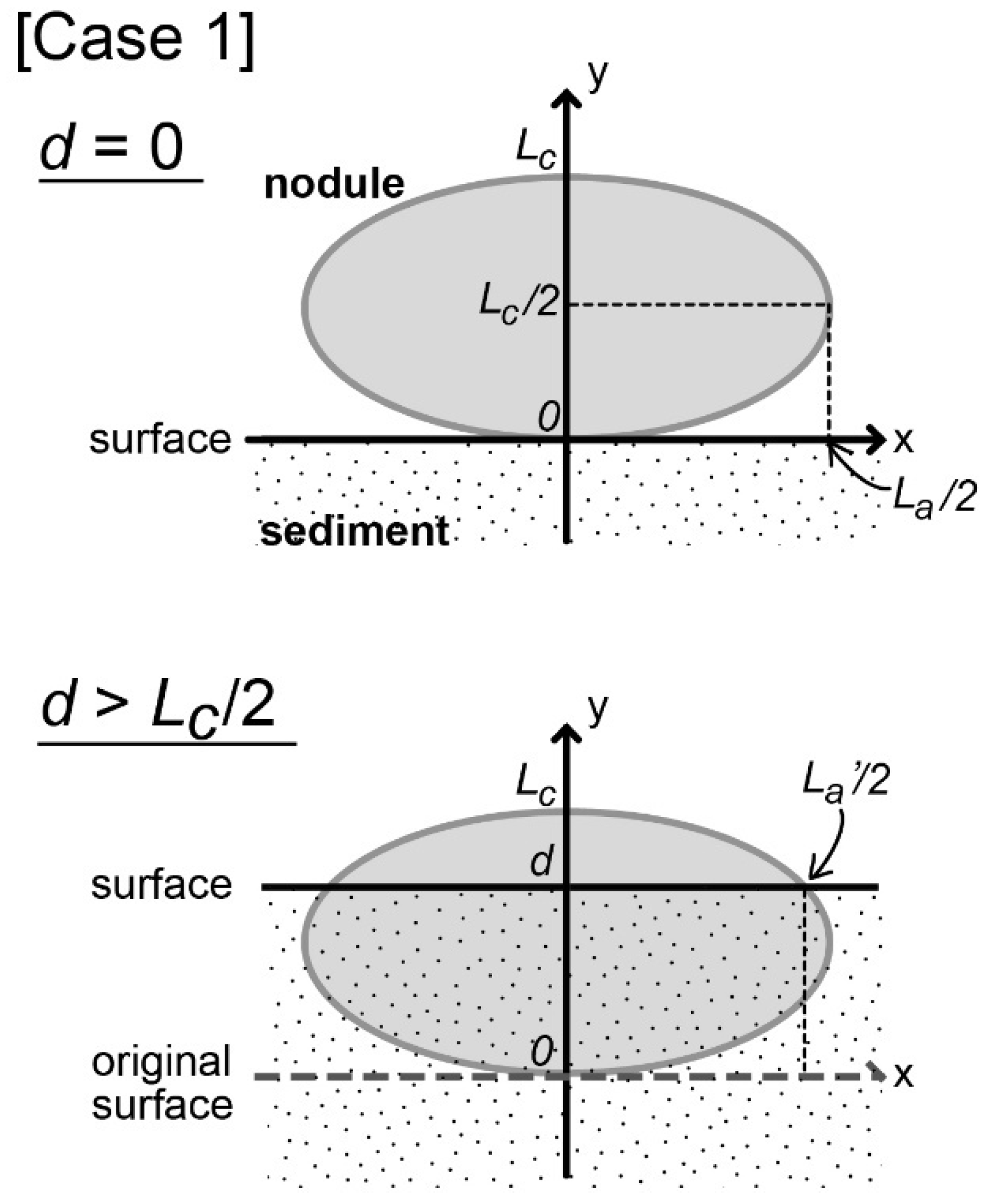
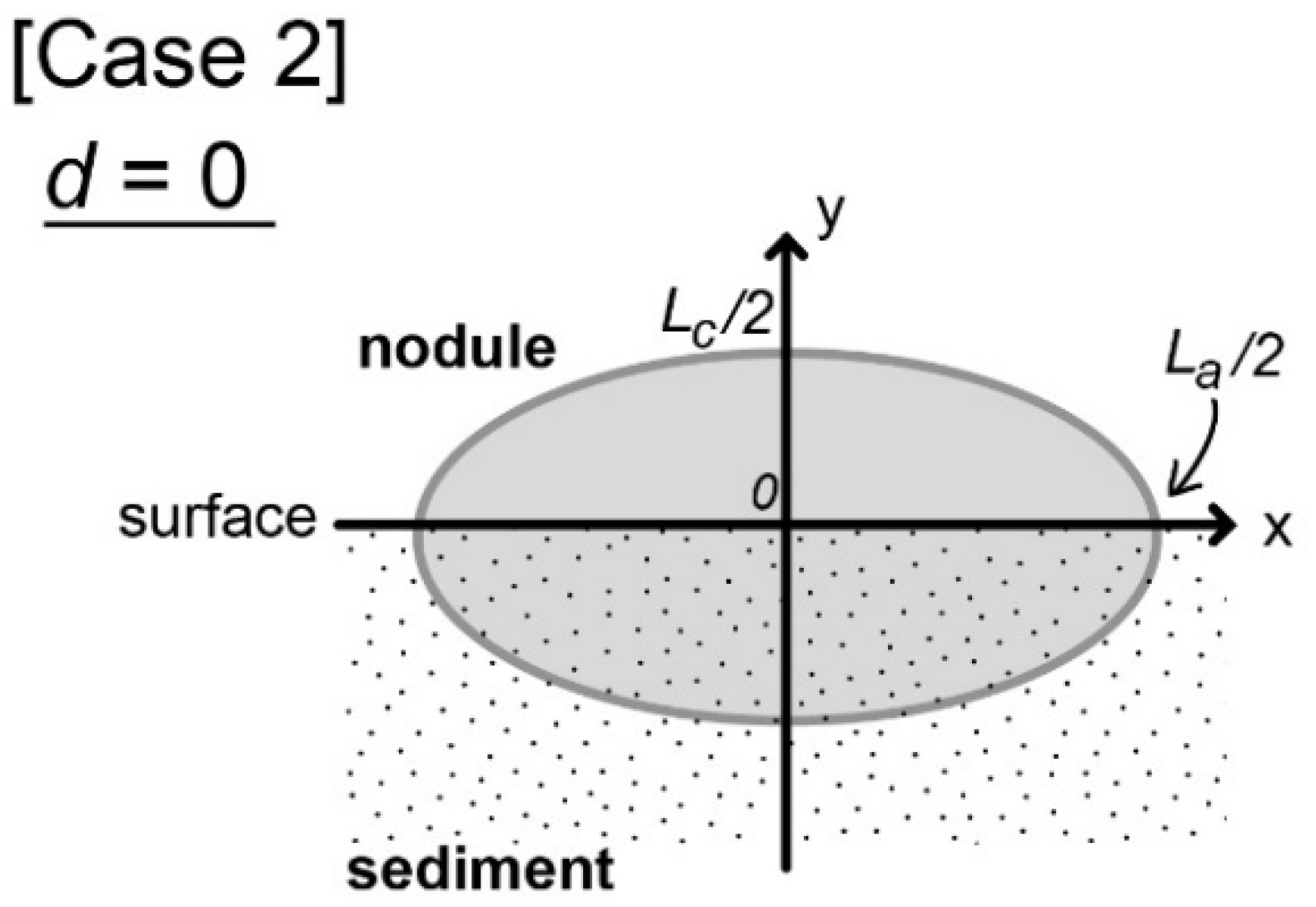
Next, the nodule configuration and burial degree are defined. Figure 2 and Figure 3 are schematic illustrations of cross sections of nodules cut in the vertical direction, which illustrate the positional relation between the nodule and sediment. These figures contain an x–y coordinate system, with the horizontal (x) axis parallel to an ideal sediment surface and the nodule’s long axis and with vertical axes (y) through the center of the nodule. The two initial conditions of positional relations between nodules and sediment are illustrated in Figure 2 and Figure 3 for Cases 1 and 2, respectively. Case 1 shows nodules in contact with the sediment, whereas Case 2 shows nodules that are individually half buried. As the actual condition before burial is unknown, these cases are used as conditions.
In this paper, burial degree is expressed as the thickness of deposits from the reference surface, that is, the sediment surface set under each case’s initial conditions. The burial degree is expressed using parameter d (unit: cm), with d = 0, meaning that the nodule configuration remains unchanged from its initial condition. For example, in Case 1, the bottoms of all the nodules come into contact the sediment at d = 0 (i.e., the sediment surface is at y = 0). If the sediment surface is shifted from y = 0 to y = d > Lc/2 by sedimentation, the exposed nodule would appear smaller as clearly shown in Figure 2 (bottom). If the magnitude of d exceeds Lc, the nodule is completely buried and appears to have disappeared from the sediment surface. Actually, although the sediment particles are expected to also fall on the top of the nodules during sedimentation, this is not considered in the present paper.
2.1. Case 1
Next, the change in nodule appearance due to burial through sedimentation is quantitatively expressed. In this case, the nodule is initially in contact with sediments. As shown in Figure 2 (top), the coordinate of the nodule’s center is (0, Lc/2).
The equation of the nodule shape, presented as an ellipse on the two-dimensional plane, is as follows:
The apparent long axis of the nodule, La′, changes with d as follows:
The relation between Lb and d can be also expressed as described above.
2.2. Case 2
Here the change in nodule appearance in Case 2, in which a half-buried nodule is considered, is quantitatively expressed (Figure 3). As the nodule’s center is the origin in this coordinate system, the equation of the ellipse can be expressed as:
The apparent long axis of the nodule, La′, changes with d as follows:
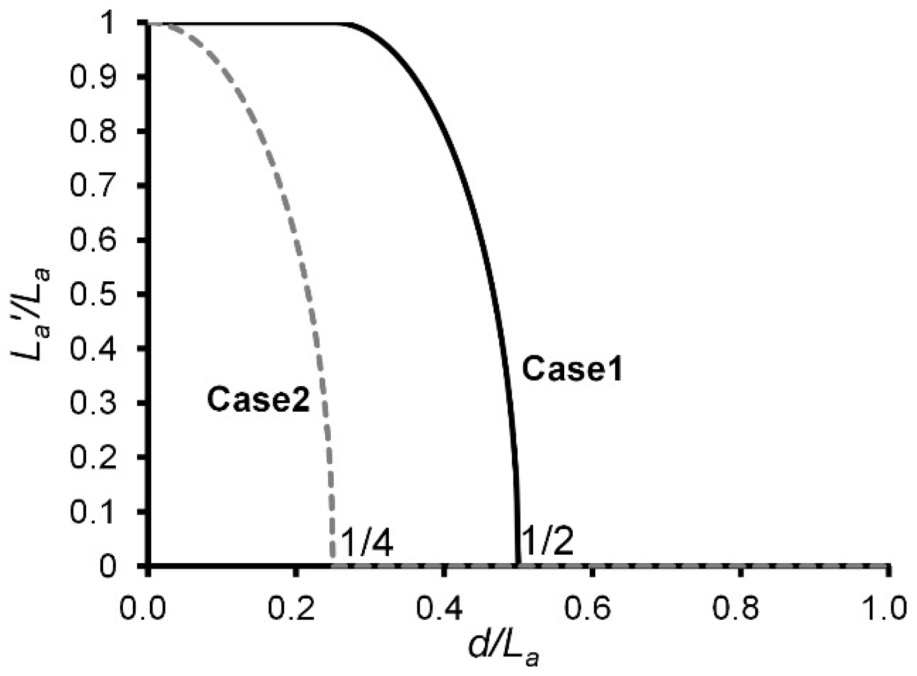
Figure 4 shows the relations between La′ and d in Cases 1 and 2. The calculations in Figure 4 assume Lc = La/2 as described in the Methods section. As the entire nodule comes into contact with the sediment under the initial condition of Case 1, nodule size does not change when d < Lc/2. In contrast, in Case 2, subtle sedimentation causes the nodule to appear smaller.
3. Methods
This section introduces a hypothetical histogram for quantitatively treating a large number of nodules. The author then shows methods and procedures of calculations to examine how various statistical values of the histogram such as total weight, average long axis, and coverage change with d. In addition, details of considerations using these calculated results are described in the Results section.
Calculation of Statistical Values for A Set of Nodules with Various Degrees of Burial
This section describes various conditions for numerical calculation of the statistical values. For simplicity, Lb = 3La/4 and Lc = La/2 [14,25], which describe a typical nodule shape, are assumed. Under these assumptions, nodule area and weight can be expressed using only La, and s and w described in model section can be rewritten to 3πLa2/16 and πLa3/8, respectively. When an aggregate of nodules is considered, the author expresses nodule size using the average long axis, L, rather than La as statistical parameters are used.
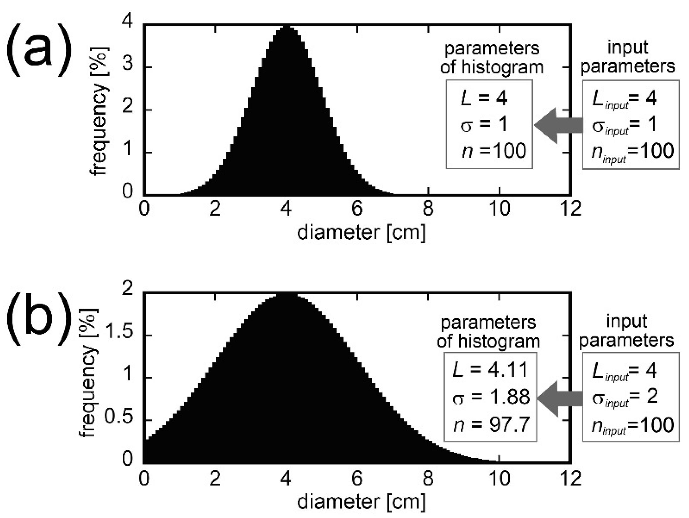
Other parameters expressing the nodule aggregate are explained. For simplicity, a discrete histogram of nodule size distribution, as used in a previous study [25], using a size class of 0.1 cm is considered. A normal distribution, an average long axis (Linput) of 2–8 cm, a standard distribution (σinput) of 0.5–4.0, and an aggregation of 100 nodules per 1 m2 are assumed to set the histogram. Table 1 summarizes these calculation conditions and the calculated parameters in addition to assumptions described above.
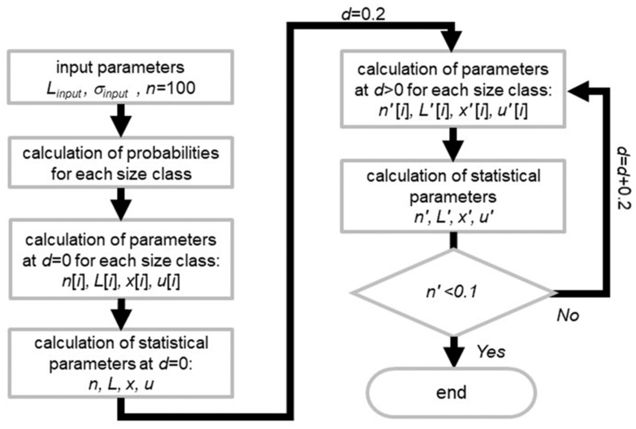
Next, procedure of the calculation is explained. First, the probabilities of each size class, L[i], are calculated based on the given values for Linput and σinput. Here, i denotes the size class, and nodules of size class i range from 0.1(i − 1) to 0.1i. For simplicity of calculation, it is assumed that all of the nodules belonging to a certain size class have the same characteristics. For example, the nodules belonging to the i = 10 size class are 0.95 cm in size (Table 1). As shown in Table 1, calculations are conducted under a range of values of i of 1–150, which covers almost all the nodules in the histogram. Although nodules with a size class smaller than zero can exist for a certain set of Linput and σinput, this study treats the probabilities of such size classes as zero considering the real situation. Therefore, the initial parameters of Linput, σinput, and n = 100 can differ from parameters in the histogram, that is, L, σ and n. Figure 5 shows examples of hypothetical histograms, which have input values that are slightly different from those of the histograms made as output. The magnitudes of these differences increase when Linput is smaller or when σinput is larger. Thus, after setting a histogram, statistical values for the distribution, such as n, L, x, and u, are calculated. Here, x means the area fraction of manganese nodules covered on the seafloor and u is calculated as the total weight of the nodules (Table 1). The n[i], L[i], x[i], and u[i] values of each size class are first calculated, after which n, L, x, and u are calculated by adding up their respective components.
For buried nodules, that is, d > 0, apparent parameters such as n′[i], L′[i], x′[i], and u′[i] of each size class are calculated first, after which L′, x′, n′, and u′ are obtained. To obtain apparent parameters under various conditions, calculation with d in increments of 0.2 (i.e., d = 0, 0.2, 0.4, …) is conducted. The calculated n′ value decreases as d increases because the number of completely buried nodules increases when deposits are thicker, as shown in Figure 1. Thus, the calculation is finished when n′ has become sufficiently small (i.e., n′ < 0.1). Figure 6 summarizes the above procedures as a flowchart.
4. Results
To elucidate model parameter changes with changing burial degree, Case 1 underwent 1303 calculations and Case 2 calculations were conducted 526 times (Table 2). Basically, the number of calculations increases with L because nodules with larger long axes need a larger d to be completely buried (i.e., for the calculations to finish).
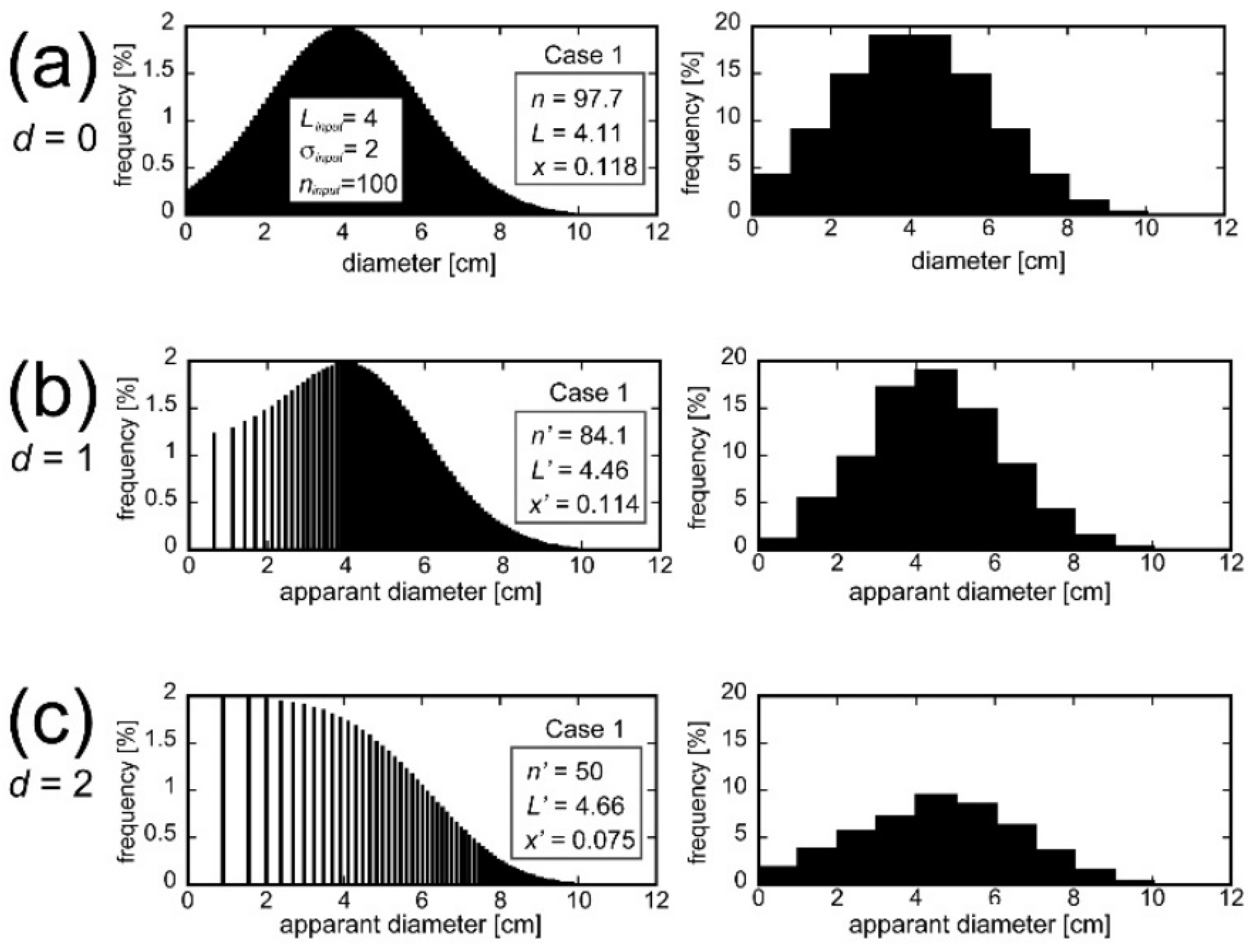
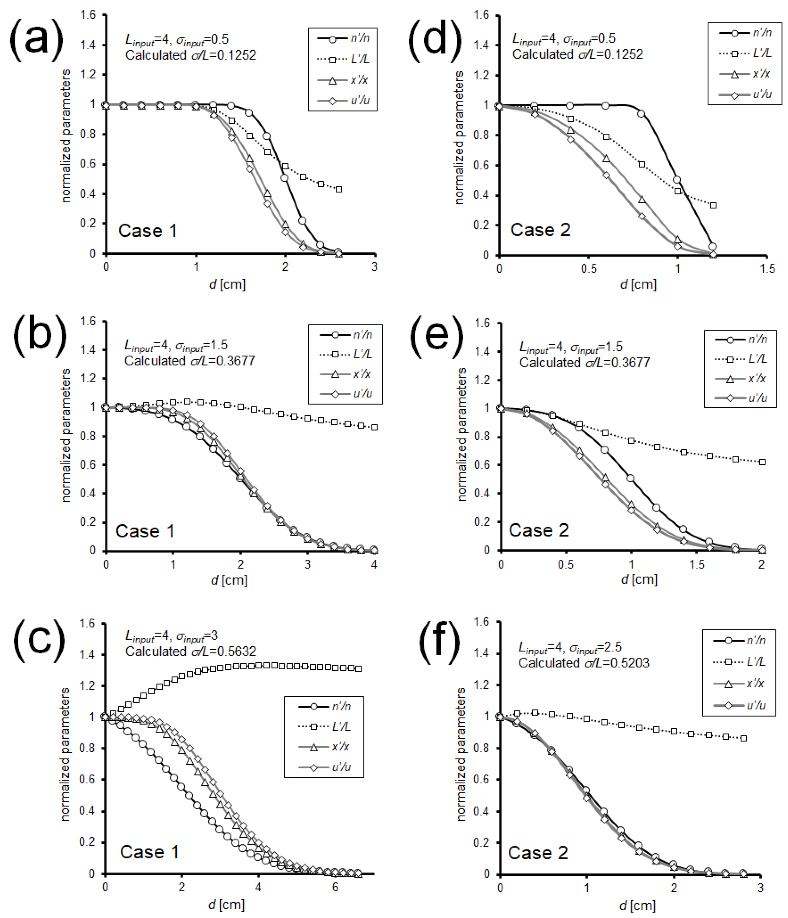
Figure 7 shows examples of histograms produced under various d (=0, 1, 2) and constant Linput (=4), σinput (=2), and n (=100) values. Figure 7 (left column) shows histograms with a size class of 0.1 cm, whereas Figure 7 (right column) redisplays them as histograms with a 1 cm size class, which would be more familiar as geological data. When d becomes larger, the left side of the histogram, that is, smaller size class nodules that are partially or completely buried, reflects the number of nodules belonging to that size class becoming smaller or zero, respectively. For these reasons, the resulting histograms in Figure 7b,c appear sparse. Furthermore, the histogram peak decreases as d increases. This trend is expressed in the histograms in Figure 7 (right column). Associated with these trends, the statistical values also change.
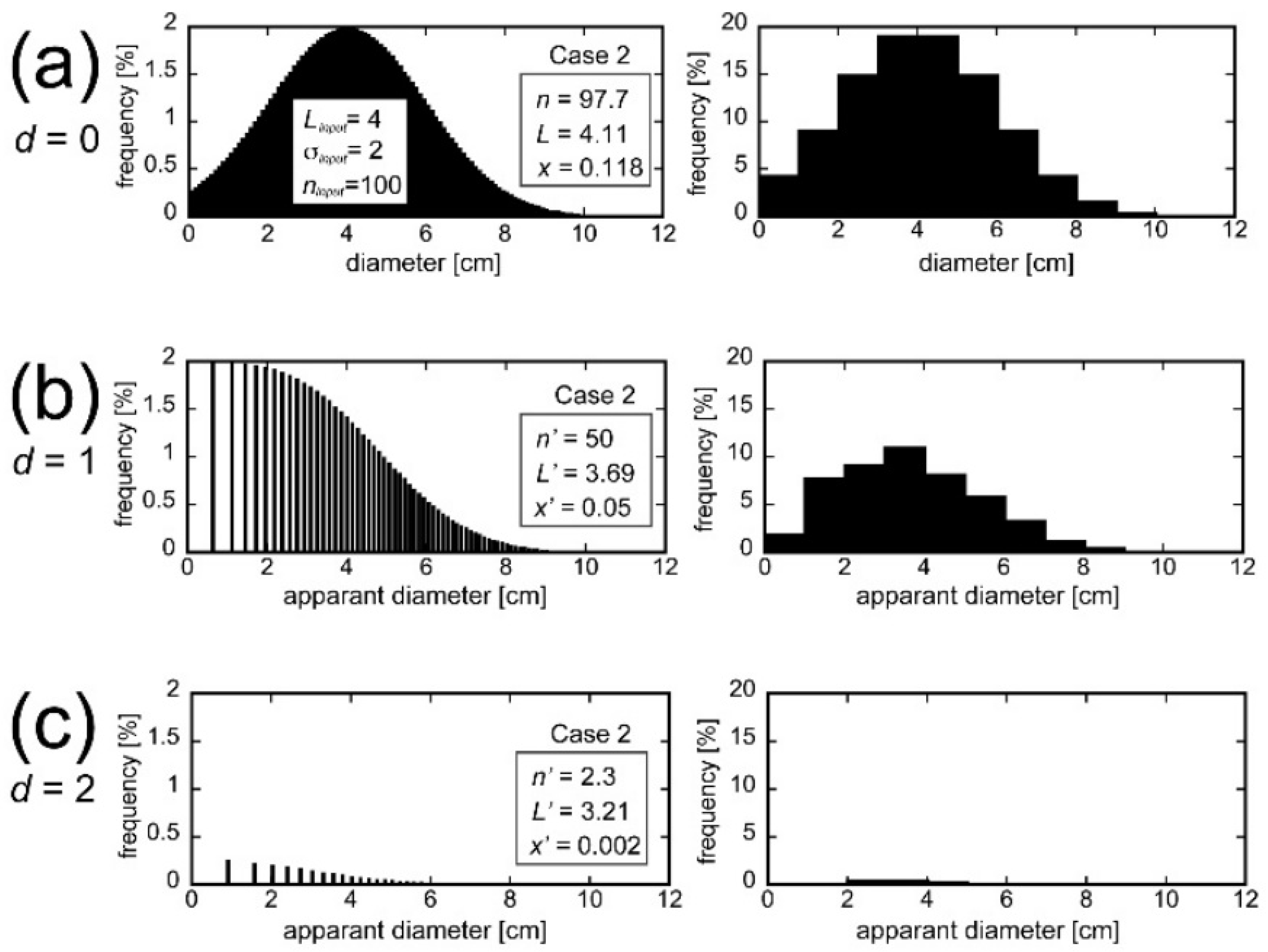
Figure 8 shows the results of calculations in Case 2, indicating that the histogram shapes change notably with d.
Figure 9 shows the relations among the normalized parameters and d. As the trends depend on σ/L, the results of several values of σ/L (~0.1–0.5) are shown as examples. Basically, n′, x′, and u′ decrease with d. Notably, the trends of x and u are similar to each other because x and u both are functions of L. For a smaller σ value, which can be expressed as a “well-sorted” nodule distribution in the field of geology, n, x, and u all decrease moderately with d. For example, most nodules are buried completely (i.e., n′ is near zero) at d = 2 (Figure 9a,d). In contrast, when σ is larger (i.e., a poorly sorted nodule distribution), the number of buried nodules is smaller for a given d. The range of L′/L also depends heavily on the magnitude of σ, especially in Case 1. When σ is smaller, L′/L ranges 0.2–1 and L′/L decreases with d (Figure 9a). For larger values of σ, L′/L increases with d and L′/L converges to 1.3 (Figure 9c). In contrast, when σ/L is near 0.4, L′/L shows almost no change with d (Figure 9b).
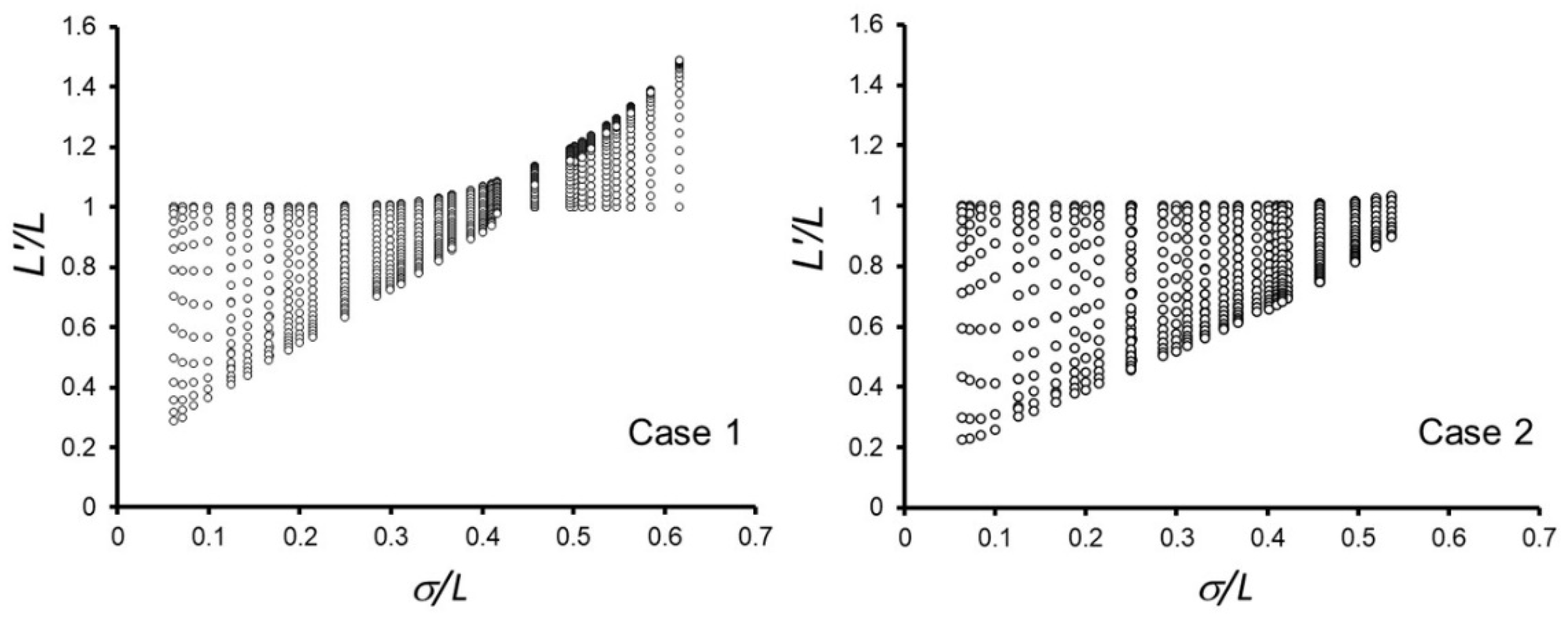
To investigate how L′ changes relative to parameter d, the range of L′ for given values of σ/L and d is summarized as expressed in a two-dimensional space in Figure 10. Each open dot represents a L′/L value calculated for a given σ/L and a given d. In Figure 10, it seems that sequences of dots line up as vertical straight lines. This shows that the results under the same σ/L are plotted on each line as shown in Figure 9. When σ is small (i.e., nodules show well-sorted distributions), L′/L ranges 0.2–1. When σ/L is near 0.4, L′/L does not change notably. When σ is large (i.e., nodules show poorly sorted distributions), L′/L increases with d as shown in Figure 9 and ranges from 1 to 1.3. These characteristics show that the behaviors of L′/L with d depend on the initial nodule distribution (parameter, σ/L).
4.1. Relation Among the Parameters
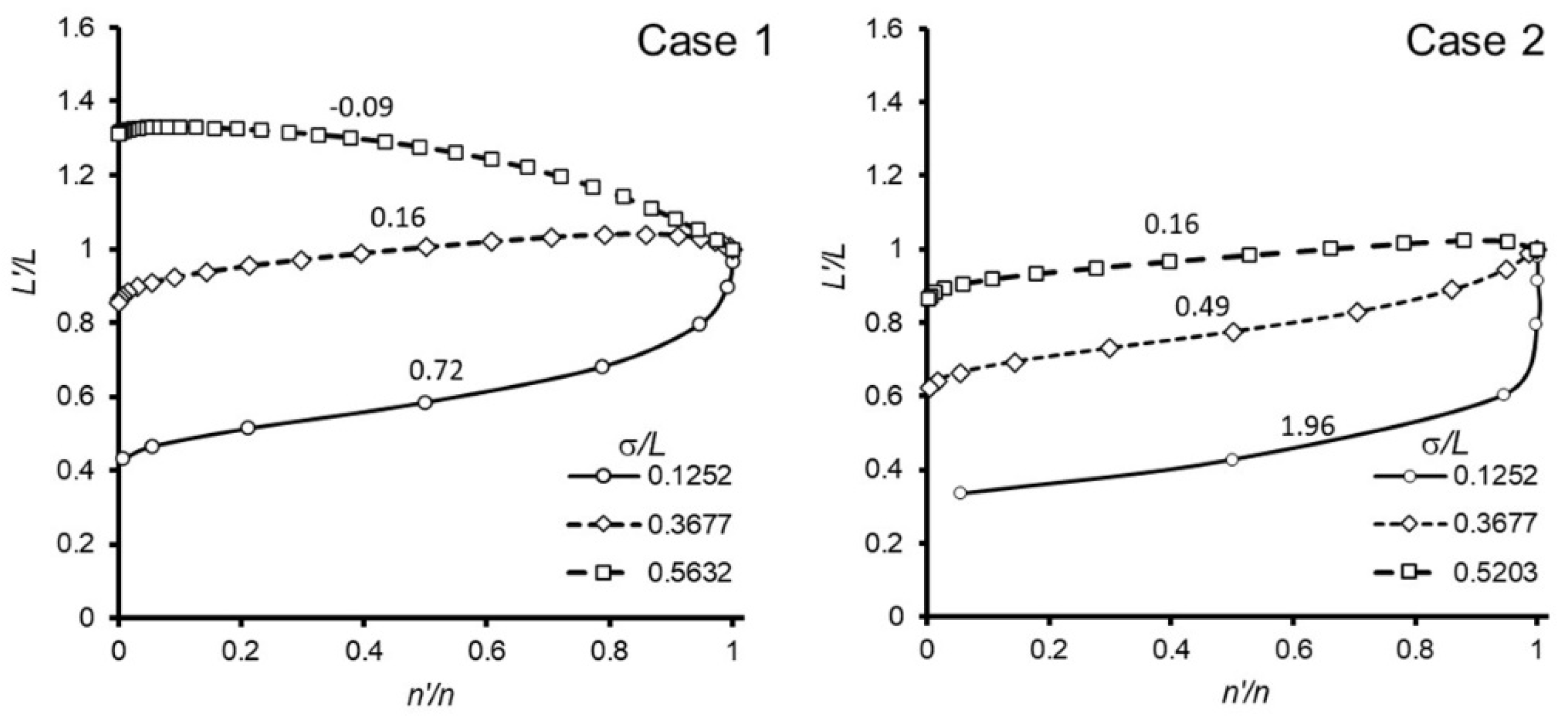
Figure 11 shows examples of the relationship between n and L at various values of σ calculated in Cases 1 and 2. Parameter d is not explicitly expressed in this figure. However, because the values of n′/n decrease with d, we can determine that trends of parameters from 1 to 0 of n′/n (horizontal axis) correspond with changes in d. For L′, as described in Figure 8, especially in Case 1, different trends exist for different σ/L values. For large values of σ/L, L/L′ increases as n/n′ decreases, whereas L/L′ decreases for small σ/L values. To quantitatively express the trend, the values of dL/dn (i.e., slope) are described near each graph. Case 1 returns −0.09–0.72 when σ/L is small and gives negative values when σ/L is large. Case 2 returns small positive values regardless of the value of σ (0.16–1.96). Thus, the range of the value of dL/dn is constrained by both case type and σ.
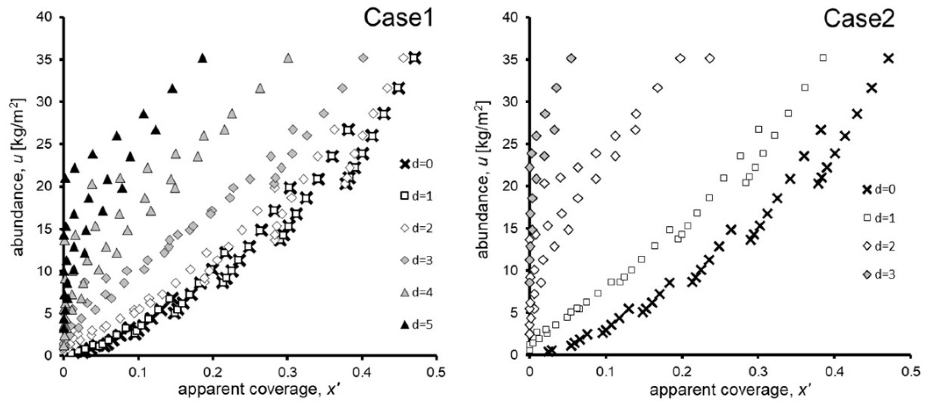
Figure 12 illustrates the relations between x′ and u in Cases 1 and 2. This plot can be found in previous studies as described in the Discussion section. The slopes of plotted points appear to be steeper with d in this figure. Additionally, some points are plotted on the y-axis for larger values of d, indicating that nodules are fully buried in this condition.
4.2. Quantitative Consideration: Relations Between α and d
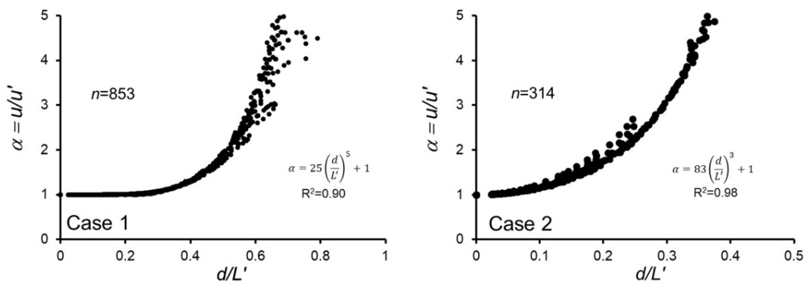
The relations between α and d/L′ is compiled from the dataset as shown in Figure 13. The value of u′ decreases with d. Therefore, α = u/u′ increases with d. Although α values of more than 1000 can be calculated, a dataset of relatively small values of α (1–5) are used in consideration of practical aspects. As shown below, fifth- and third-order equations of d/L′ are obtained by fitting these datasets for Cases 1 and 2, respectively (Figure 13).
Table 3 shows the degrees of nodule abundance underestimation due to burial, which can be expressed as 1/α. These degrees are calculated using the above two fitting equations. Additionally, the estimated nodule abundances become half of the real abundances for d/L′ = 0.53 under Case 1 and d/L′ = 0.23 under Case 2.
4.3. Quantitative Consideration: C-factor in An Empirical Equation
In addition to showing the relationship between the C-factor in Equation (1) and the newly defined α, this paper will quantify that relationship using the dataset. The C-factor reflects a variety of factors, such as burial degree and nodule shape and this is determined by L′, x′ measured from a seabed photograph in addition to actual abundance data. To separate the burial degree from the C-factor, the following equation is introduced:
This resembles Equation (1), which shows the relations among L, x (not L′ and not x′), and u. c0 is defined as c without a burial factor. Additionally, by introducing to the ratio of the burial, α = u/u′, Equations (1) and (2) can be rewritten as follows:
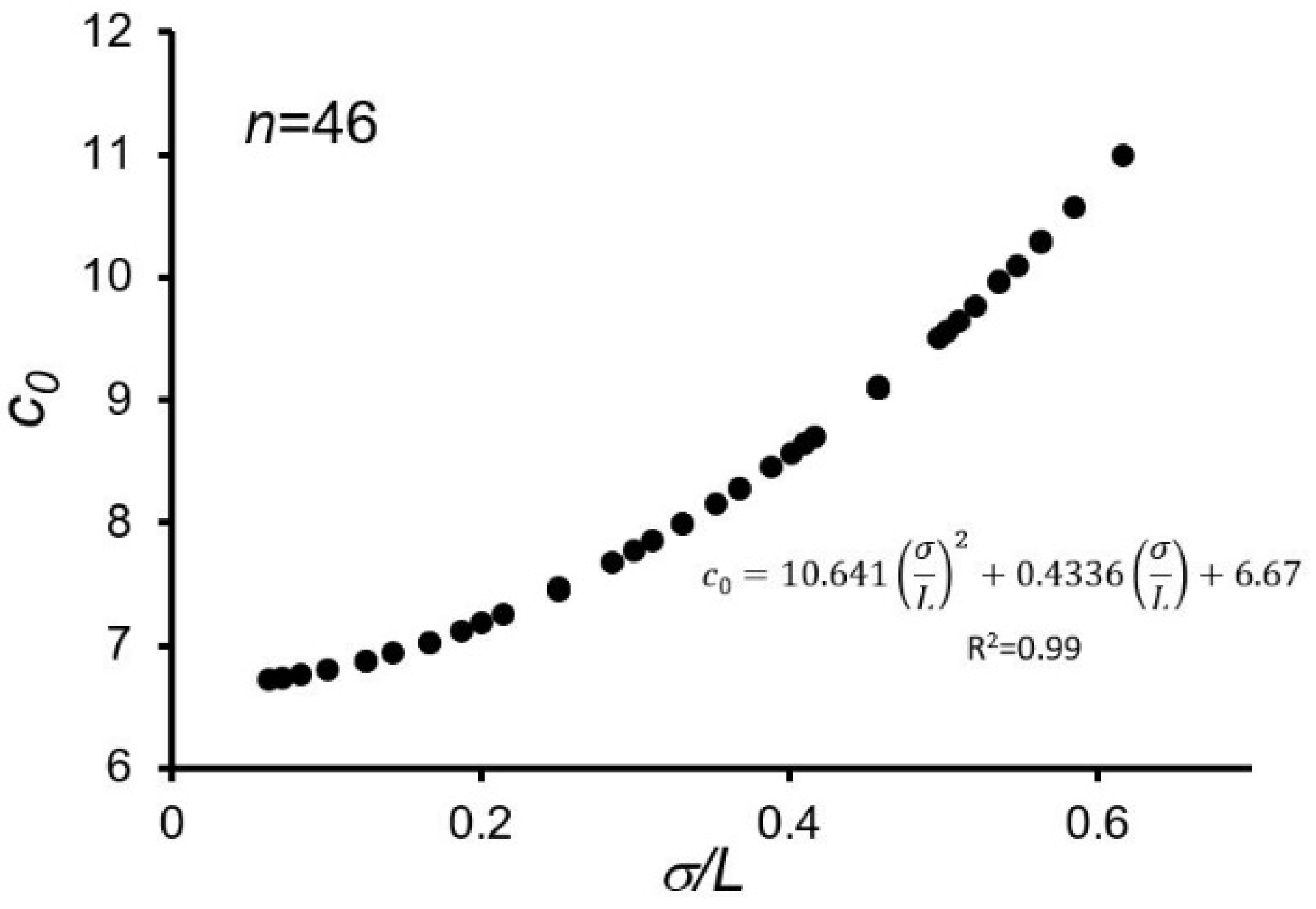
Assuming that there are no other factors of c0 not dealt with in the present paper, the relation between the c0 values and σ/L can be obtained by compiling the results calculated among the dataset for d = 0. That is, in Equation (2), c0 is obtained by calculating u/(Lx) for the dataset at d = 0. As u, L, and x depend on σ and L (i.e., histogram shape), c0 was expressed as a function of these parameters through regression. Figure 14 shows the relation between c0 values and σ/L, and the fitting equation is expressed as:
For the plot shown in Figure 14, the results of 46 calculations for the dataset at d = 0 in Case 1 are used. When creating the fitting equation, the coefficients of the quadratic equation of σ/L were determined solely from the dataset, whereas the intercept for σ/L = 0 (i.e., the value of c0 when all nodules have equal size) was set to 6.67 [25]. The maximum value of c0 under this condition is approximately 11.
5. Discussion
5.1. Calculation Results
This paper investigates the dependence of the parameters of manganese nodules extracted from seafloor photographs or video on d. A previous study [13] showed qualitative relations between deposit thickness and nodule characteristics, and those relations have been reproduced quantitatively by calculations in this study. As d increases, the number of exposed nodules (n′) and apparent coverage (x′) observed on the seafloor both decrease (Figure 8 and Figure 9). However, the calculations in this study demonstrate that the trend of L′ is complicated. This is because the burial of small nodules can result in an increase in L′ in some cases, whereas the burial of large nodules results in decreased values of L′. Figure 9c or Figure 10 show a strange trend in which L′ increases with d only when σ is large in Case 1.
The relation between n′ and L′ can be found in Figure 11. Particularly, because both n′ and L′ are parameters that can be measured from seafloor photographs, a dataset of n′ and L′ values obtained from a large number of consecutively taken seafloor photographs may be used as an indicator to determine whether nodule burial occurs notably in an area of interest.
Figure 12 shows the relationship between x′ and u and has been used in previous studies (e.g., [17]) to investigate the varieties of nodules sampled in a vast area. This paper demonstrated that the trends of the u vs. x′ plot regularly change based on the burial degree, and Figure 12 shows that slopes reproduced under each condition become steeper when d is larger. These indicate that magnitudes of the slope of a regression line made by ground-truth data, which directly related to the C-factor, can indirectly express information on d in areas of interest.
5.2. Assumptions and Conditions Used in Modeling and Simulation
Various assumptions and conditions were used to calculate parameter dependence on nodule burial degree. For example, based on the previous studies [14,25], manganese nodule shape is assumed to be a practical case. A normal distribution is adopted for the nodule size distribution. In fact, because nodule shape and distribution in the deep seafloor are not simple, it is necessary to pay attention when applying these results. However, the author considers that an examination based on these assumptions is valid to understand quantitative relations among parameters as a first trial.
Moreover, this study includes primitive examinations; therefore, some problems remain. For example, some previous studies [13,26] have indicated that not only buried nodules look smaller but also can appear to be divided into two or more nodules, a phenomenon known as a fractionation effect [13]. The appearance of divided nodules results in an increase of the apparent number of nodules, which may change trends as seen in Figure 10. Thus, the actual trend will deviate from the trend shown in Figure 10. However, regularity of the fractionation effect is complicated; thus, this paper does not consider this effect.
As the initial conditions of manganese nodule configuration, two cases (Cases 1 and 2) are considered. However, unknown factors related to nodule burial manner remain. One of the possibilities of the model is that nodules may be randomly buried, and regularities such as dependence on nodule size may not be found in the nodules. However, in this case, it is impossible to define d, and changing the parameter is very simple. For example, L′ does not depend on burial degree, and the values of u′ and x′ are decided only by the number (proportion) of buried nodules. Therefore, this paper omits this case.
5.3. Nodule Burial Phenomenon
A geological description of the burial phenomenon suitable for actual situations is a task for future work. Previous studies have discussed that the diversity of manganese nodule abundance could be attributable to the sediment covering nodules, that is, burial degree [13,14,26]. Sediments contributing to manganese nodule burial near the surface, an area known as the sediment–water interface boundary [26], are unconsolidated deposits. A previous study indicated that coverage in this layer results in apparent smaller nodule size and measured the relative thickness of the sediment–water interface boundary that was qualitatively determined based on a photograph of the burial of the trigger weight attached to the sampler and examined the relation between sediment thicknesses and nodule abundance [26]. However, this study shows that nodule size apparently increases with burial degree under limited conditions (Figure 10).
In contrast, some studies performed descriptions related to burial phenomenon. For example, because nodule surface roughness has been considered as an indicator of an environment for nodule growth, details on roughness may provide information that is indirectly related to burial degree (e.g., [17,21,27,28]). Additionally, the resolution of the image used to measure nodule size also affects the measurement of burial degree [7]. On a separate note, a biological study measured the burial degree for sampled nodules and sediments to investigate the microhabitat of organisms on the nodules [29]. However, descriptions for geological studies do not seem to have progressed.
5.4. Quantitative Consideration: Relation Between α and d
This paper investigated how the value of α quantitatively relates to d. Figure 13 shows the relationship between d (normalized as d/L) and α. Burial degree is represented by α and is a simply increasing function of d/L (Figure 13). This figure shows that a small value of d indicates values close to 1, with a tendency for d to increase exponentially. The calculations in this paper demonstrate that burial factors significantly affect estimated abundance. For example, assuming L = 4, when d/L is 0.25, α = 1.5 (Case 1) or 2 (Case 2). Additionally, the calculations indicate that α strongly depends on initial conditions. As shown in Table 3, the impact of burial is significant in Case 2. A previous study [14] noted that the maximum is 50%, which corresponds roughly to d = 2 for Case 1 and d = 1 for Case 2 (L′ = 4). This range of d values may be the maximum value of d in reality except in cases where nodules are completely buried.
5.5. Quantitative Consideration: C-factor in An Empirical Equation
As α can be directly obtained from sampling data and photos, it is useful to examine whether α can be also inferred from existing published data. Additionally, to understand the origin of nodule formation, it is common to consider data over a wide area and examine the regularity of those data. However, this does not seem to have been sufficiently conducted. Equation (1) was improved to Equation (3), in which α was obviously expressed. The parameter c0 in Equation (3), which does not affect burial degree, is also expressed as a function of L and σ (Figure 14). The newly defined value of c0 can be calculated from the formula in Figure 14, allowing the calculation of α from c0 and c. The constant term in the three-dimensional fitting equation drawn in Figure 14 (i.e., 6.67) is the minimum value of c0 when σ = 0, that is, when all manganese nodules are of the same size [25]. Data of σ/L = 0.0–0.6 were used, and the maximum value of the C-factor (αc0) is ~11 under these conditions (Figure 14). Thus, it is expected that separating the burial from the C-factor contributes to a more precise estimation of the mineral resource.
C-factors much greater than 11 have been reported [24], meaning that the burial degree of manganese nodules in the area of interest (a certain area in the Indian Ocean) is large (i.e., α > 1) or the nodules have morphologies similar to a spherical form. In contrast, a C-factor of 7.7 in an area in the Pacific Ocean has been reported [30], indicating a much smaller burial degree (i.e., α ~ 1) or that the shapes of nodules in the survey area are more planar. Ground-truth data are needed to determine whether it is nodule shape or burial degree that predominantly determines C-factor values. However, in any case, the values derived from compiled data such as the C-factor can be useful in discussing the origin of nodules in the area. Although it is important to note that features of burial degree can vary by area, it would be useful to compile data from this perspective in the future. Additionally, it should be noted that the best quantification of burial can vary depending on the data in the target area. For example, as shown in Figure 12, in the case with larger d, many apparent coverages are zero or close to zero for different nodule abundances. This suggests that it may be difficult to express using an empirical equation such as Equation (3). In contrast, the author considers that the u–x′ plots shown in Figure 12, which are related to the C-factor, can provide useful geological information as a first trial.
5.6. Application to Understanding Manganese Nodule Origins
A large number of seafloor images have been captured in recent years, and the variety of image analysis methods is growing. However, studies concerning burial phenomena have been insufficient, and this study is expected to contribute to further understanding nodule genesis and improve resource estimation. Image data taken continuously in recent AUV surveys can take one photo every few seconds, acquiring data at intervals of several meters [10,22]. Additionally, improvement and automation of computer programs that identify manganese nodules and estimate resource amounts have been advanced heavily [6,8,9]. However, burial’s effects do not seem to be considered in these programs, nor is it considered in the analysis of images captured in large quantities. It is not easy to directly determine burial degree from seafloor photographs; however, investigating the tendencies of multiple parameters against a seafloor photograph (Figure 11) is a possible analysis method.
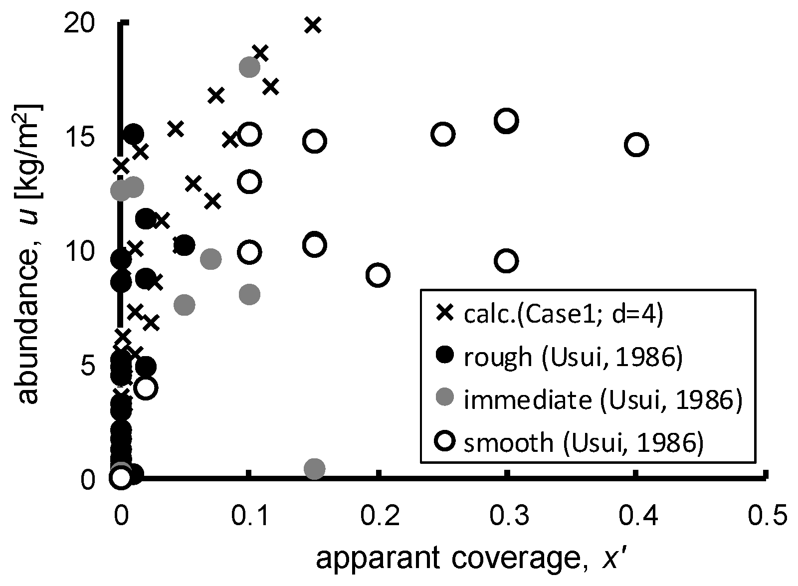
Additionally, two parameters related to burial, d and α, are thought to be useful for understanding the geological genesis of manganese nodules as these parameters are indirectly related to sediment deposition rate. For example, manganese nodules with rough surfaces have been identified as being characteristic of buried manganese nodules (e.g., [17,31]). It has been shown that the spatial distribution concerning this roughness reflects the diversity of the sedimentation rate affected by ocean topography or bottom flow (e.g., [1,3,15,18,19,20]), and a recent study illustrated that bottom currents control sedimentation [32]. The author considers that introducing the burial degree to quantify such studies is one research direction. Figure 15 shows the abundance and apparent coverage of manganese nodules in the Central Pacific as measured by the Geological Survey of Japan [27], with results calculated for Case 1 and d = 4 overlaid on the figure. Although the relationship between direct burial measurement data and burial degree defined in this study is not discussed in detail, Figure 15 shows that fully or almost buried nodules (i.e., coverage x′ ~ 0) have rough surfaces and that the calculation results can reproduce the trend of rough nodules. Parameter d may represent the distribution of the nodule. Thus, one direction of future research of deep seafloor manganese nodules can be that the examined area is characterized by parameter d.
However, it is also possible that the relationship between burial degree and the individual geological characteristics of manganese nodules varies in different waters (e.g., Peru Basin [33] and Central Pacific Basin [17]). Therefore, caution is needed when applying the relationships obtained in one area to other areas. Additionally, it is necessary to keep in mind that burial is one of factors that dominates manganese nodule genesis and that determine the morphological features. For example, in the case of nodules that are less buried (e.g., around Minami–Torishima Island [34]), parameters other than burial degree may be more important for understanding nodule origins. In addition, taking into account types of genesis such as hydrogenetic, diagenetic and hydrogenetic–diagenetic are also important to estimate nodule abundance precisely from seabed photographs and to study the geological origin [35,36]. Since these types of genesis have been mainly studied by approaches of chemical analysis including measurement of oxic conditions in pore water within sediment (e.g., [2,3,15,16,35,37]), an interdisciplinary approach will make a great contribution to understand the origin of nodules.
Although outside the scope of this paper, importance of the geological description for manganese nodules themselves remains unchanged in studying the genesis. For example, previous reports show that the top, bottom, and side surfaces of nodules have different roughness and textures and that nodules have different characteristics for different local topography of sea areas (e.g., [3,18,28]). Thus, the author considers that it is also important to describe geologically nodules with their complex structures in addition to collecting the seafloor photographs.
6. Conclusions
To quantify the burial degree of manganese nodules in seafloor sediments, the sediment thickness from the reference plane, d, and the ratio of the weight to the apparent weight of the manganese nodule, α, are introduced. Calculations were performed to clarify how the apparent parameters change with d for a hypothetical nodule size distribution. This paper clarified the following:
- The tendency of the parameters that change depending on the burial degree as mentioned in a previous study was reproduced using numerical calculations;
- The calculations basically show that u′, x′, and n′ decrease with increasing values of d, but L′ takes various behaviors depending on conditions, though the trend of L′ is similar to those of u′, x′, and n′ under most conditions;
- The relationship between the hypothetical parameter, d, and the actual measurable parameter, α, was formulated, resulting in α being represented as a third-order or fifth-order function of d/L′;
- Improving an empirical equation to estimate nodule abundance from seafloor photographs, a coefficient known as the C-factor was re-expressed as a product of α and c0. Furthermore, c0 was represented by a two-dimensional equation of parameter σ/L using a dataset. Using the published C-factor and some geological conditions, α in the area of interest can be estimated.
Funding
This research received no external funding.
Acknowledgments
This study is conducted as part of projects entrusted by the Ministry of Economy, Trade and Industry. The author would also like to thank the anonymous reviewers and the editors for providing valuable comments which helped improve this manuscript.
Conflicts of Interest
The author declares no conflict of interest of interest.
References
- Frazer, J.Z.; Fisk, M.B. Geological factors related to characteristics of sea-floor manganese nodule deposits. Deep Sea Res. Part A Oceanogr. Res. Pap. 1981, 28, 1533–1551. [Google Scholar] [CrossRef]
- Morgan, C.L. Resource estimates of the Clarion-Clipperton manganese nodule deposits. In Handbook of Marine Mineral Deposits; Cronan, D.S., Ed.; CRC Press: Boca Raton, FL, USA, 2000; pp. 145–170. [Google Scholar]
- Kuhn, T.; Wegorzewski, A.; Rühlemann, C.; Vink, A. Composition, formation, and occurrence of polymetallic nodules. In Deep-Sea Mining; Sharma, R., Ed.; Springer: Cham, Germany, 2017; pp. 23–63. [Google Scholar] [CrossRef]
- Hein, J.R.; Koschinsky, A.; Kuhn, T. Deep-ocean polymetallic nodules as a resource for critical materials. Nat. Rev. Earth Environ. 2020, 1, 158–169. [Google Scholar] [CrossRef]
- Wright, I.C.; Graham, I.J.; Chang, S.W.; Choi, H.; Lee, S.R. Occurrence and Physical Setting of Ferromanganese Nodules Beneath the Deep Western Boundary Current, Southwest Pacific Ocean. N. Z. J. Geol. Geophys. 2005, 48, 27–41. [Google Scholar] [CrossRef]
- Sharma, R.; Sankar, S.J.; Samanta, S.; Sardar, A.A.; Gracious, D. Image analysis of seafloor photographs for estimation of deep-sea minerals. Geo-Mar. Lett. 2010, 30, 617–626. [Google Scholar] [CrossRef]
- Tsune, A.; Okazaki, M. Some Considerations about Image Analysis of Seafloor Photographs for Better Estimation of Parameters of Polymetallic Nodule Distribution. In Proceedings of the 24th International Ocean and Polar Engineering Conference, Busan, Korea, 15–20 June 2014; International Society of Offshore and Polar Engineers: Cupertino, CA, USA, 2014; pp. 72–77. [Google Scholar]
- Schoening, T.; Kuhn, T.; Jones, D.O.B.; Simon-Lledo, E.; Nattkemper, T.W. Fully Automated Image Segmentation for Benthic Resource Assessment of Poly-Metallic Nodules. Methods Oceanogr. 2016, 15, 78–89. [Google Scholar] [CrossRef]
- Schoening, T.; Jones, D.O.B.; Greinert, J. Compact-Morphology-Based Poly-Metallic Nodule Delineation. Sci. Rep. 2017, 7, 13338. [Google Scholar] [CrossRef] [PubMed]
- Peukert, A.; Schoening, T.; Alevizos, E.; Köser, K.; Kwasnitschka, T.; Greinert, J. Understanding Mn-Nodule Distribution and Evaluation of Related Deep-Sea Mining Impacts Using AUV-Based Hydroacoustic and Optical Data. Biogeosciences 2018, 15, 2525–2549. [Google Scholar] [CrossRef] [Green Version]
- Jung, H.S.; Ko, Y.T.; Chi, S.B.; Moon, J.W. Characteristics of seafloor morphology and ferromanganese nodule occurrence in the Korea Deep-sea Environmental Study (KODES) Area, NE Equatorial Pacific. Mar. Georesour. Geotechnol. 2001, 19, 167–190. [Google Scholar] [CrossRef]
- UNOET (U. N. Ocean Economics and Technology Branch). Assessment of Manganese Nodule Resources: The Data and Methodologies; Graham and Trotman, Ltd.: London, UK, 1982. [Google Scholar]
- Sharma, R. Effect of sediment-water interface ‘boundary layer’ on exposure of nodules and their abundance: A study from seabed photos. J. Geol. Soc. India 1989, 34, 310–317. [Google Scholar]
- Bastien-Thiry, H. Sampling and surveying techniques. In Manganese Nodules: Dimensions and Perspectives; The United Nations Ocean Economics and Technology Office, Ed.; Reidel: Dodrecht, The Netherlands, 1979; pp. 7–19. [Google Scholar]
- Kuhn, T.; Uhlenkott, K.; Vink, A.; Rühlemann, C.; Arbizu, P.M. Manganese nodule fields from the Northeast Pacific as benthic habitats. In Seafloor Geomorphology as Benthic Habitat; Harris, P.T., Baker, E., Eds.; Elsevier: Amsterdam, The Netherlands, 2020; pp. 933–947. [Google Scholar] [CrossRef]
- Wegorzewski, A.V.; Kuhn, T. The influence of suboxic diagenesis on the formation of manganese nodules in the Clarion Clipperton nodule belt of the Pacific Ocean. Mar. Geol. 2014, 357, 123–138. [Google Scholar] [CrossRef]
- Usui, A.; Nishimura, A.; Tanahashi, M.; Terashima, S. Local variability of manganese nodule facies on small abyssal hills of the Central Pacific Basin. Mar. Geol. 1987, 74, 237–275. [Google Scholar] [CrossRef]
- Skornyakova, N.S.; Murdmaa, I.O. Local variations in distribution and composition of ferromanganese nodules in the Clarion-Clipperton Nodule Province. Mar. Geol. 1992, 103, 381–405. [Google Scholar] [CrossRef]
- Piper, D.Z.; Blueford, J.R. Distribution, mineralogy, and texture of manganese nodules and their relation to sedimentation at DOMES Site A in the equatorial North Pacific. Deep Sea Res. Part A Oceanogr. Res. Pap. 1982, 29, 927–951. [Google Scholar] [CrossRef]
- Sharma, R.; Kodagali, V.N. Influence of seabed topography on the distribution of manganese nodules and associated features in the Central Indian Basin: A study based on photographic observations. Mar. Geol. 1993, 110, 153–162. [Google Scholar] [CrossRef]
- Usui, A.; Moritani, T. Manganese nodule deposits in the Central Pacific Basin: Distribution, geochemistry, mineralogy, and genesis. In Geology and Offshore Mineral Resources of the Central Pacific Basin; Springer: New York, NY, USA, 1992; pp. 205–223. [Google Scholar] [CrossRef]
- Okazaki, M.; Tsune, A. Exploration of Polymetallic Nodule Using AUV in the Central Equatorial Pacific. In Proceedings of the 10th ISOPE Ocean Mining and Gas Hydrates Symposium, Szczecin, Poland, 22–26 September 2013; International Society of Offshore and Polar Engineers: Cupertino, CA, USA, 2013; pp. 32–38. [Google Scholar]
- Gazis, I.Z.; Schoening, T.; Alevizos, E.; Greinert, J. Quantitative mapping and predictive modeling of Mn nodules’ distribution from hydroacoustic and optical AUV data linked by random forests machine learning. Biogeosciences 2018, 15, 7347–7377. [Google Scholar] [CrossRef] [Green Version]
- Sharma, R.; Khadge, N.H.; Jai Sankar, S. Assessing the Distribution and Abundance of Seabed Minerals from Seafloor Photographic Data in the Central Indian Ocean Basin. Int. J. Remote Sens. 2013, 34, 1691–1706. [Google Scholar] [CrossRef]
- Tsune, A. Effects of size distribution of deep-sea polymetallic nodules on the estimation of abundance obtained from seafloor photographs using conventional formulae. In Proceedings of the 11th Ocean Mining and Gas Hydrates Symposium, Kona, HI, USA, 21–27 June 2015; International Society of Offshore and Polar Engineers: Cupertino, CA, USA, 2015; pp. 153–159. [Google Scholar]
- Sharma, R. Quantitative estimation of seafloor features from photographs and their application to nodule mining. Mar. Georesour. Geotechnol. 1993, 11, 311–331. [Google Scholar] [CrossRef]
- Usui, A. Local variability of manganese nodule deposits around the small hills in the GH81-4 area. Geol. Surv. Jpn. Cruise Rept. 1986, 21, 98–159. [Google Scholar]
- Nishi, K.; Koizumi, A.; Tsune, A.; Tanaka, S. A Preliminary Study of the Relation Between Topographic Features and the Distribution of Polymetallic Nodules in Japanese License Area, Central Pacific. In Proceedings of the 28th International Ocean and Polar Engineering Conference, Sapporo, Japan, 10–15 June 2018; International Society of Offshore and Polar Engineers: Cupertino, CA, USA, 2018; pp. 69–73. [Google Scholar]
- Veillette, J.; Juniper, S.K.; Gooday, A.J.; Sarrazin, J. Influence of surface texture and microhabitat heterogeneity in structuring nodule faunal communities. Deep Sea Res. Part I Oceanogr. Res. Pap. 2007, 54, 1936–1943. [Google Scholar] [CrossRef] [Green Version]
- Handa, K.; Tsurusaki, K. Manganese nodules: Relationship between coverage and abundance in the northern part of Central Pacific Basin. Deep Sea Mineral Resources Investigation in the Northern Part of Central Pacific Basin. Geol. Surv. Jpn. Cruise Rept 1981, 15, 184–217. [Google Scholar]
- Raab, W. Physical and chemical features of Pacific deep sea manganese nodules and their implications to the genesis of nodules. In Ferromanganese Deposits on the Ocean Floor; Horn, D.R., Ed.; National Science Foundation: Alexandria, VA, USA, 1972; pp. 31–49. [Google Scholar]
- Juan, C.; Van Rooij, D.; De Bruycker, W. An assessment of bottom current controlled sedimentation in Pacific Ocean abyssal environments. Mar. Geol. 2018, 403, 20–33. [Google Scholar] [CrossRef]
- von Stackelberg, U. Manganese nodules of the Peru Basin. In Handbook of Marine Mineral Deposits; Cronan, D.S., Ed.; CRC Press: Boca Raton, FL, USA, 2000; pp. 197–238. [Google Scholar]
- Machida, S.; Fujinaga, K.; Ishii, T.; Nakamura, K.; Hirano, N.; Kato, Y. Geology and geochemistry of ferromanganese nodules in the Japanese Exclusive Economic Zone around Minamitorishima Island. Geochem. J. 2016, 50, 539–555. [Google Scholar] [CrossRef] [Green Version]
- Halbach, P.; Scherhag, C.; Hebisch, U.; Marchig, V. Geochemical and Mineralogical Control of Different Genetic Types of Deep-Sea Nodules from the Pacific Ocean. Miner. Depos. 1981, 16, 59–84. [Google Scholar] [CrossRef]
- Wasilewska-Błaszczyk, M.; Mucha, J. Possibilities and Limitations of the Use of Seafloor Photographs for Estimating Polymetallic Nodule Resources—Case Study from IOM Area, Pacific Ocean. Minerals 2020, 10, 1123. [Google Scholar] [CrossRef]
- Sasmaz, A.; Zagnitko, V.M.; Sasmaz, B. Major, trace and rare earth element (REE) geochemistry of the Oligocene stratiform manganese oxide-hydroxide deposits in the Nikopol, Ukraine. Ore Geol. Rev. 2020, 126, 103772. [Google Scholar] [CrossRef]
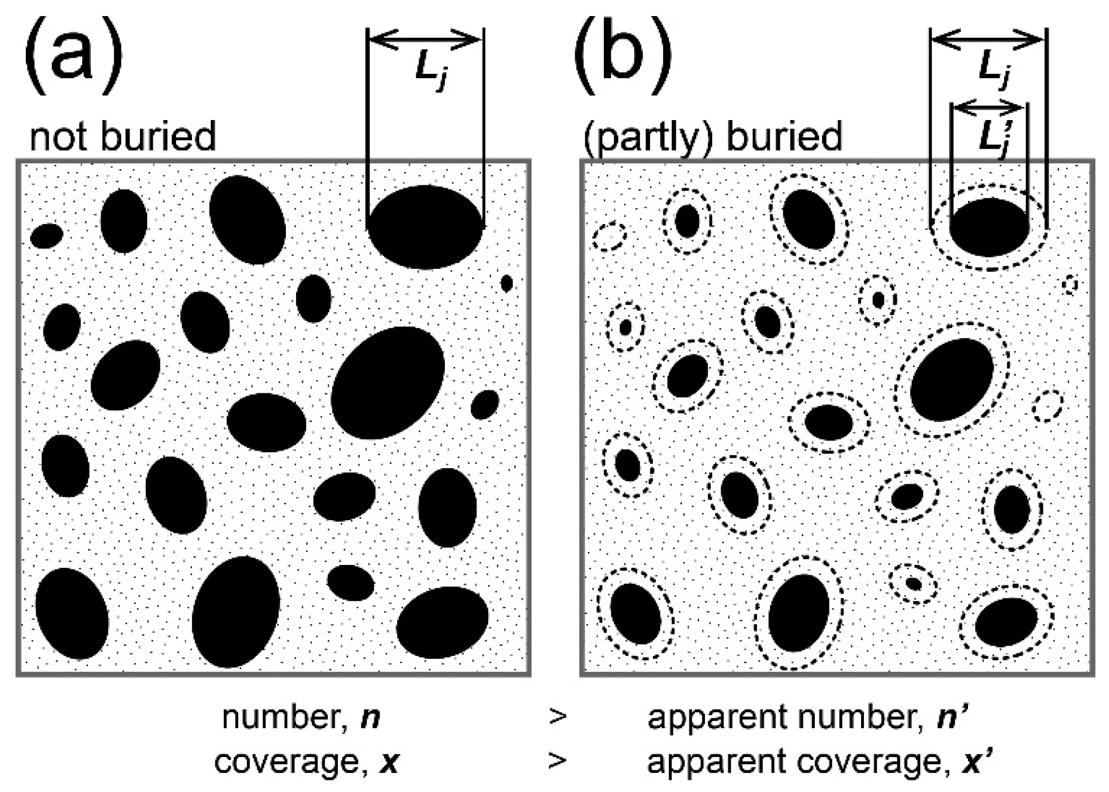
Figure 1.
Schematic illustrations of manganese nodules on the deep seafloor (original illustration is from [13]). (a) Nodules not covered by sediments (or with a lower degree of burial). (b) Nodules heavily covered by sediments (or with a higher degree of burial). In case (b), the apparent long axis of large nodules (Lj′) becomes smaller than that of original nodules (Lj), and small nodules are completely buried (j means an identified number). The dotted circles surrounding each nodule show the outlines of unburied nodules. Further, comparing between (a) and (b), apparent number (n′) and coverage (x′) of nodules per area unit also become smaller than those of original nodules (n, x), respectively.

Figure 2.
Schematic illustration of a cross section of a nodule and sediment that shows positional relations for Case 1. The hypothetical nodule has long axis of La and thickness of Lc. The bottom of the nodule comes into contact with the sediment under the initial condition (d = 0). When d > Lc/2, the nodule’s apparent size is smaller, as shown in the bottom part of the figure.

Figure 3.
Schematic illustration of a cross section of a nodule and sediment that shows positional relations for Case 2. The nodule is half-buried into sediment under the initial condition.
Figure 3.
Schematic illustration of a cross section of a nodule and sediment that shows positional relations for Case 2. The nodule is half-buried into sediment under the initial condition.

Figure 4.
Relations between d and L in Cases 1 and 2.

Figure 5.
Examples of hypothetical histograms. Large Linput and small σinput values result in the same outputs of L and σ as shown in (a). That is, the statistical parameters of histograms are unchanged. However, in the other cases, the input values are different from those of the histogram as shown in (b) because a portion of the smaller size class is eliminated.

Figure 6.
Flowchart of the calculation procedure. Many rounds of calculations are needed for larger nodules because the condition of n′ < 0.1 is achieved when d is larger.
Figure 6.
Flowchart of the calculation procedure. Many rounds of calculations are needed for larger nodules because the condition of n′ < 0.1 is achieved when d is larger.

Figure 7.
Histograms showing the results of calculations for various d values in Case 1. (a) d = 0; (b) d = 1; (c) d = 2. See text for details.
Figure 7.
Histograms showing the results of calculations for various d values in Case 1. (a) d = 0; (b) d = 1; (c) d = 2. See text for details.

Figure 8.
Histograms showing calculation results for various values of d in Case 2. (a) d = 0; (b) d = 1; (c) d = 2. See text for details.
Figure 8.
Histograms showing calculation results for various values of d in Case 2. (a) d = 0; (b) d = 1; (c) d = 2. See text for details.

Figure 9.
Relations among normalized variables and d in (a–c) Case 1 and (d–f) Case 2. Each plot represents the output of parameters calculated using given Linput, σinput, and d as shown in the flowchart in Figure 6.
Figure 9.
Relations among normalized variables and d in (a–c) Case 1 and (d–f) Case 2. Each plot represents the output of parameters calculated using given Linput, σinput, and d as shown in the flowchart in Figure 6.

Figure 10.
Behaviors of L with respect to d in Cases 1 and 2. The ranges of L′ for a variety of σ values are shown, and these parameters are normalized by L. Lengthwise sets of dots represent L′ calculated for a given σ and various values of d.
Figure 10.
Behaviors of L with respect to d in Cases 1 and 2. The ranges of L′ for a variety of σ values are shown, and these parameters are normalized by L. Lengthwise sets of dots represent L′ calculated for a given σ and various values of d.

Figure 11.
Relation between L′ and n′ in Cases 1 and 2. Numbers near each line are the average slopes (dL/dn).
Figure 11.
Relation between L′ and n′ in Cases 1 and 2. Numbers near each line are the average slopes (dL/dn).

Figure 12.
Relation between abundance u and apparent coverage x′ in Cases 1 and 2. The calculated results for various values of d are plotted.
Figure 12.
Relation between abundance u and apparent coverage x′ in Cases 1 and 2. The calculated results for various values of d are plotted.

Figure 13.
Relation between d and α in Cases 1 and 2.

Figure 14.
Relation between c0 (i.e., C-factor when d = 0) and σ/L.

Figure 15.
Relation between x′ and u. Crosses indicate nodule abundances calculated under conditions with Case1 and d = 4. Circles indicates ground-truth data of nodule abundances in Central Pacific Ocean [27]. Different colors of the circles mean different roughness of surface for nodules collected at each location.


Table 1.
Calculation conditions, assumptions and parameters of the histogram used in this paper.
| Assumptions or Conditions on Nodules or the Histogram | Parameters of the Histogram | ||
|---|---|---|---|
| Items | Assumptions or Conditions | Parameters | Equations |
| shape of each nodule | ellipsoidal | For size class i | |
| (minor axis)/(major axis) = 3/4 | number | ||
| (thickness)/(major axis) = 1/2 | (representative) long axis [cm] | ||
| number of the size class | i = 1, 2, …, 150 | area (per a nodule) [cm2] | |
| range of each size class [cm] | [0.1 (i − 1), 0.1i] | weight (per a nodule) [g] | |
| size distribution of nodules | normal distribution | For histogram | |
| parameters: Linput, σinput and ninput | number of nodule per 1 m2 | ||
| probability for each size class: | average long axis [cm] | ||
| p[i] | coverage (proportion covered by nodules per 1 m2) | ||
| abundance [kg/m2] (total weight of nodules per 1 m2) | |||
Table 2.
Number of calculations and conditions used.
| Linput | σinput | Range of d [cm] | Number of Calculation | |
|---|---|---|---|---|
| Case 1 | 2 to 8 | 0.5 to 4.0 | 0 to 7.8 | 1303 |
| Case 2 | 2 to 8 | 0.5 to 3.5 | 0 to 4.8 | 526 |
Table 3.
Underestimation of nodule abundance due to burial. 1/α represents the proportion of underestimation of the estimated abundance due to burial.
Table 3.
Underestimation of nodule abundance due to burial. 1/α represents the proportion of underestimation of the estimated abundance due to burial.
| d/L′ | |||||||
|---|---|---|---|---|---|---|---|
| 0.05 | 0.1 | 0.15 | 0.2 | 0.25 | 0.3 | ||
| 1/α | Case1 | <0.1% | <0.1% | 0.2% | 0.8% | 2.4% | 5.7% |
| Case2 | 1.0% | 7.7% | 21.9% | 39.9% | 56.5% | 69.1% | |
Publisher’s Note: MDPI stays neutral with regard to jurisdictional claims in published maps and institutional affiliations. |
© 2021 by the author. Licensee MDPI, Basel, Switzerland. This article is an open access article distributed under the terms and conditions of the Creative Commons Attribution (CC BY) license (http://creativecommons.org/licenses/by/4.0/).
Share and Cite
MDPI and ACS Style
Tsune, A. Quantitative Expression of the Burial Phenomenon of Deep Seafloor Manganese Nodules. Minerals 2021, 11, 227. https://doi.org/10.3390/min11020227
AMA Style
Tsune A. Quantitative Expression of the Burial Phenomenon of Deep Seafloor Manganese Nodules. Minerals. 2021; 11(2):227. https://doi.org/10.3390/min11020227
Chicago/Turabian StyleTsune, Akira. 2021. "Quantitative Expression of the Burial Phenomenon of Deep Seafloor Manganese Nodules" Minerals 11, no. 2: 227. https://doi.org/10.3390/min11020227
Note that from the first issue of 2016, this journal uses article numbers instead of page numbers. See further details here.