
Reducing the Dimensions of the Stochastic Programming Problems of Metallurgical Design Procedures


Escuela de Ingeniería Química, Pontificia Universidad Católica de Valparaíso, Valparaíso 2340000, Chile
Minerals 2021, 11(12), 1302; https://doi.org/10.3390/min11121302
Submission received: 27 October 2021
/
Revised: 17 November 2021
/
Accepted: 19 November 2021
/
Published: 23 November 2021
(This article belongs to the Special Issue Modeling, Design and Optimization of Multiphase Systems in Minerals Processing, Volume II)
Abstract
:Process design procedures under uncertainty result in stochastic optimization problems whose resolution is complex due to the large uncertainty space, which hinders the application of optimization approaches, as well as the establishment of relationships between input and output variables. On the other hand, supervised machine learning (SML) offers tools with which to develop surrogate models, which are computationally inexpensive and efficient. This paper proposes a procedure based on modern design of experiments, deterministic optimization, SML tools, and global sensitivity analysis (GSA) to reduce the size of the uncertainty space for stochastic optimization problems. The proposal is illustrated with a case study based on the stochastic design of flotation plants. The results reveal that surrogate models of stochastic formulation enable the prediction of the structure, profitability parameters, and metallurgical parameters of designed flotation plants, as well as reducing the size of the uncertainty space via GSA and, consequently, establishing relationships between the input and output variables of the stochastic formulation.
1. Introduction
The procedures proposed in previous research for process design are commonly based on mathematical programming, which exhibits the following characteristics: first, it implements a superstructure to represent design alternatives from which a set of optimal alternatives can be selected; second, it uses mathematical expressions to model design alternatives, constraints, and goals. The mathematical model results in mixed-integer nonlinear programming (MINLP) or mixed-integer linear programming (MILP) problems; third, it uses an algorithm to solve the design problem from the previous stage. The procedure described above has been applied to design flotation circuits [1], reverse osmosis plants [2], desalinated water distribution systems [3], heap leaching circuits [4], and extraction solvent plants [5], among others. This approach assumes that the parameters are known; however, in practice, uncertainties are prevalent in industrial processes due to inaccurate measurement, forecast error, or lack of information, and these effects on process output variables could be critical.
Optimization under uncertainty must deal with a large uncertainty space that generally leads to large-scale optimization models that, when added to integer decision variables, constraints, and multiple objectives of the model, significantly increase the execution time and computational burden. Traditional research proposes a variety of philosophies to address optimization under uncertainty, such as stochastic programming, fuzzy mathematical programming, and stochastic dynamic programming, among others. These approaches commonly offer conservative solutions for the stochastic design problem due to the large uncertainty space, among other aspects. A review of these approaches can be found in [6] and their applications for mineral processing in [7,8,9]. An alternative, “less elegant” approach to the study of the effect of uncertainty on the optimization is proof by exhaustion. This is a mathematical proof in which the statement to be proved is split into a limited number of cases, and each case is checked separately to see if the proposition in question holds. This approach has been applied to confirm the following postulate: “there are a finite set of optimal structures when flotation systems are designed under uncertainty” [10,11]. The proof by exhaustion requires a moderate-scale optimization problem, ideally linear, to obtain responses in a reasonable time and to avoid the collapse of random-access memory (RAM). These authors implemented several assumptions to reduce the computational burden of the design problem. For example, processing stages were modeled using distribution functions, and profitability parameters, such as capital expenditures (CAPEX), operating expenditures (OPEX), net present value (NPV), profits (PROF), and net cash flow (NCF) were not considered. These profitability parameters require knowledge of the size of the equipment in each flotation stage, the amount of equipment in each flotation stage, the time of residence in each flotation stage, and the lifetime of the project, among other features, which increase the computational burden. On the other hand, some researchers have addressed metallurgical process design under uncertainty reactively via local sensitivity analysis [12] and global sensitivity analysis [13]. From the literature review, the following emerges: first, it is desirable to reduce the uncertainty space to favor the application of stochastic optimization approaches; second, establishing a relationship between the input and output variables of the design problem is complex due to the large uncertainty space; third, it is unfeasible to apply analysis in stochastic programming problems due to the large uncertainty space. Fortunately, in the age of machine learning (ML), their tools have come to help us to develop surrogate models computationally inexpensive and efficient. They are focused on endowing programs with the ability to learn and adapt, and can be classified according to the training type: supervised, non-supervised, and reinforcement [14]. In particular, supervised training requires labeled data samples to approximate mapping to predict output values or data labels, and it can be divided into regression and classification. Thus, supervised ML (SML) offers tools to construct surrogate models via regression and classification problems, such as artificial neural networks, support vector machines, Gaussian process, and AdaBoost, among others, which could be implemented to replace MINLP or MILP problems under uncertainty. The integration of SML tools and mathematical optimization has been reported in previous research to replace rigorous models in MINLP/MILP problems [15,16,17,18] raised from design procedures, optimization under uncertainty [19], surrogate modeling of stochastic simulators to perform sensitivity analysis [20], and to overcome MINLP problems in the dynamic optimization of sequential batch processes [21]; however, its application in metallurgical process design has not been reported.
This manuscript presents a methodology to reduce the uncertainty space of stochastic programming problems, which emerge from design procedures. This paper considers four stages: first, defining a stochastic optimization problem; second, replacing the stochastic problem by deterministic problems via a design of experiment, and solving each one separately; third, constructing surrogate models using the information collected in previous stage and SML tools; and fourth, subjecting the surrogate models to global sensitivity analysis to reduce the uncertainty space of the stochastic formulation. The methodology proposed is illustrated using a design procedure for flotation circuits under uncertainty. The codes utilized in this study were developed in JupyterLab, using the python kernel, and they are attached as Supplementary Materials.
2. Methods
2.1. Modern Design of Experiments (MDoE)
Design of Experiments (DoE) is a branch of statistics that helps designers plan, execute, and analyze tests to evaluate process responses. DoE can be divided into two families: classical and modern experiment design. The first is based on laboratory experiments; examples of this category are factorial design, central composite design, and the Box–Behnken design. The second is based on computer simulations to replace expensive physical experiment with faster and cheaper computer simulations. These DoEs use different space-filling strategies to empirically capture the behavior of the underlying system over a limited range of variables [22].
2.2. Supervised Machine Learning (SML)
Machine learning is a branch of artificial intelligence that aims to extract knowledge from data. ML algorithms can build models based on data to perform predictions (i.e., regression problems) or make decisions (i.e., classification problems). In a classification problem, the algorithm is trained to approximate a correlation between the input data and output label/category, whereas in a regression problem, the output variable is a real value. In this study, the surrogate model is represented by classification and regression models [23]. The SML tools selected to address regression problems were the multilayer perceptron (MLP), support vector regression (SVR), random forest regression (RFR), the linear model (LM), ridge model (RM), lasso model (LM), and elastic net model (ENM). The SML tools selected to address classification problems were the multilayer perceptron classifier (MLPC), support vector classifier (SVC), AdaBoost classifier (ABC), Gaussian process classifier (GPC), and Gaussian Naïve Bayes classifier (GNBC). A review of these tools can be seen in [24].
2.3. Global Sensitivity Analysis (GSA)
This considers evaluating the output variable variability contemplating the input variables in their uncertainty domains. GSA can be performed using different approaches, such as screening methods, linear regression-based methods, and variance decomposition-based methods, among others [25]. Those based on variance decomposition are highlighted due to their efficiency and versatility. The Sobol–Jansen method belongs to this category and enables the determination of the first-order sensitivity index and the total sensitivity index for each input variable of the model. The first-order index allows the determination of the most important input variable, while the total index allows the identification of the input variables that do not influence the output variable. Note that the Sobol–Jansen method has been implemented to analyze mining processes; interested readers can find some applications in [13,26]
2.4. Generic Framework to Reduce the Uncertainty Space
The computational framework used to reduce the uncertainty space considers four stages. First, a stochastic optimization problem must be defined from design procedures. Second, the uncertainty space of stochastic optimization problem must be sampled using a form of MDoE, such as Latin hypercube sampling, symmetric sampling, and orthogonal array sampling, among other techniques. Next, the stochastic optimization problem must be replaced by deterministic problems and each one solved separately using exact algorithms, such as BARON solver, included in General Algebraic Modeling System software (GAMS development corporation, Fairfax, VA, USA). The information collected must be processed to eliminate outliers, balancing the dataset, and removing unavailable values, among other procedures. Third, the processed dataset and SML tools must be used to construct surrogate models via classification and regression problems. Note that classification problems are defined via the labeling of structures of designed processes. The quality of surrogate models can be determined using metrics, such as the mean squared error (MSE), R-squared (), mean absolute error (MAE), and root mean squared error (RMSE) for regression or accuracy, precision, sensitivity, and specificity for classification. Programing languages, such as Julia, Python, Rstudio, and Matlab, or integrated development environments, such as JupyterLab and Pycharm can be used to construct surrogate models. Fourth, surrogate models obtained from the regression problems must be subjected to GSA, subsequently reducing the uncertainty space and establishing relationships among input and output variables.
3. Applications
The methodology proposed is illustrated using a procedure implemented to design flotation plants. This procedure is based on mathematical programming and considers the following aspects: first, a superstructure representing 2304 alternatives of design that include five flotation stages, splitters, and mixers; second, a mathematical model including mass balance, a bank model to estimate mineralogical species recoveries, and several objective functions, among other specifications, which results in a MINLP problem; for more detail, see [27]. The uncertainty space of the MINLP problem is formed by twenty input variables, which can be seen in Table 1.
The uncertainty can be classified as stochastic and epistemic; the first is related to the variation inherent in a given system and is present in the deposit grade, feed conditions, kilowatt-hours, and copper price; the second derives from a lack of knowledge of the system and is present in operational aspects, such as the number of cells. In this study, the input variables (1–15) exhibited stochastic uncertainty and, according to previous research, the uncertainty could be described with normal distribution functions (see Table 1). The number of cells (16–20) presented epistemic uncertainty and, according to the Principle of Indifference, its uncertainty could be expressed with uniform distribution functions, in this case, discrete functions (see Table 1).
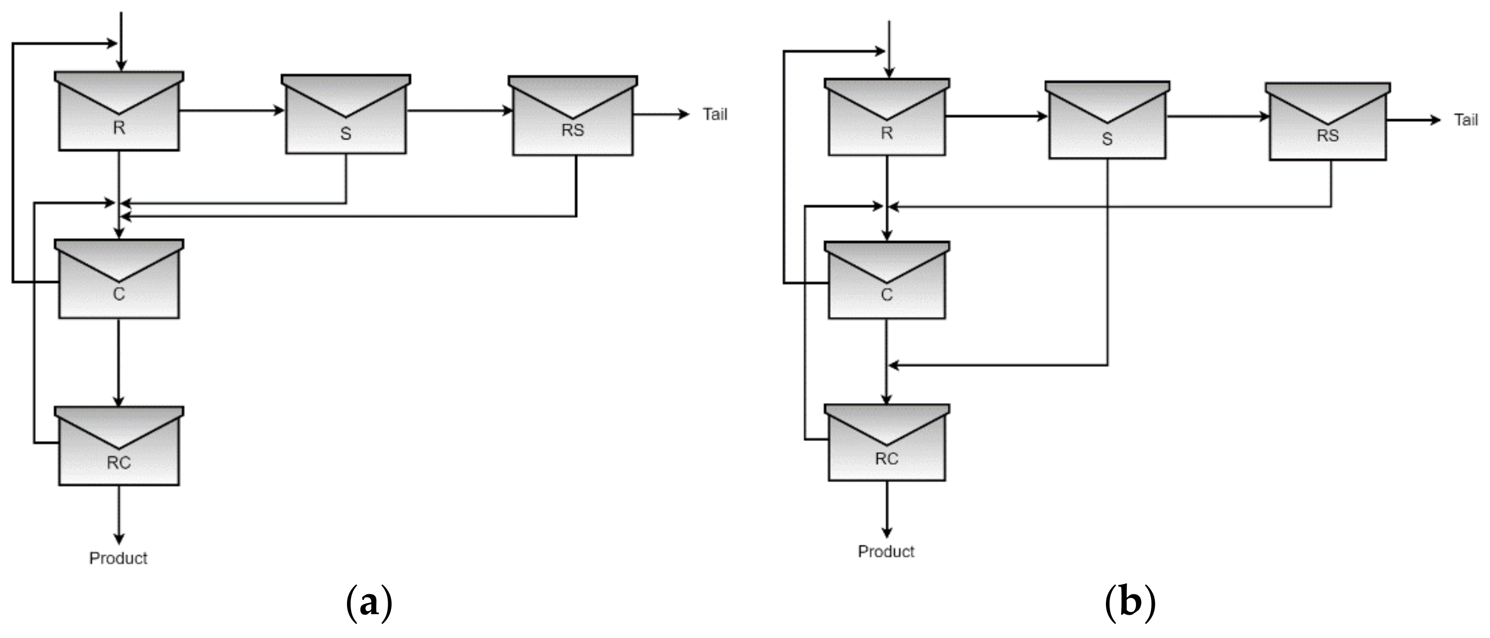
This study focused on two scenarios: the first considers an uncertainty space formed by fifteen input variables (1–15); the second considers an uncertainty space formed by twenty input variables (1–20). The uncertainty space was sampled five hundred times using the Latin-Hypercube method; subsequently, the results were utilized to replace the stochastic formulation with deterministic problems. The objective function selected was maximizing NPV because it includes metallurgical, operational, and profitability parameters, whereas the output variables of the design problem included plant structure, CAPEX, OPEX, PROF, NCF, revenue (REV), and copper grade and recovery for the designed flotation plants. A computer with Intel Core i7 2.21 GHz and 16 GB of RAM and BARON solver included in GAMS software (release 30.1.0) was implemented to solve the deterministic problems. The execution times for the first and second scenario were 82,800 s and 7200 s, respectively, and both scenarios presented two predominant structures, which can be seen in Figure 1.
The difference in execution time could be related to the flotation model used to estimate mineralogical species recoveries, specifically, in the interaction between the number of cells and residence time in each flotation stage [28]. The dataset obtained in the previous stage was processed to remove noise, outliers, unavailable values, and balancing of the dataset. Subsequently, the processed dataset was charged in JupyterLab to construct surrogate models using the sklearn library [29]. Here, classification problems were considered to predict the designed plant structures, whereas regression problems predicted profitability and metallurgical parameters for the designed plants. Figure 2 and Figure 3 show the results obtained for classification and regression problems.
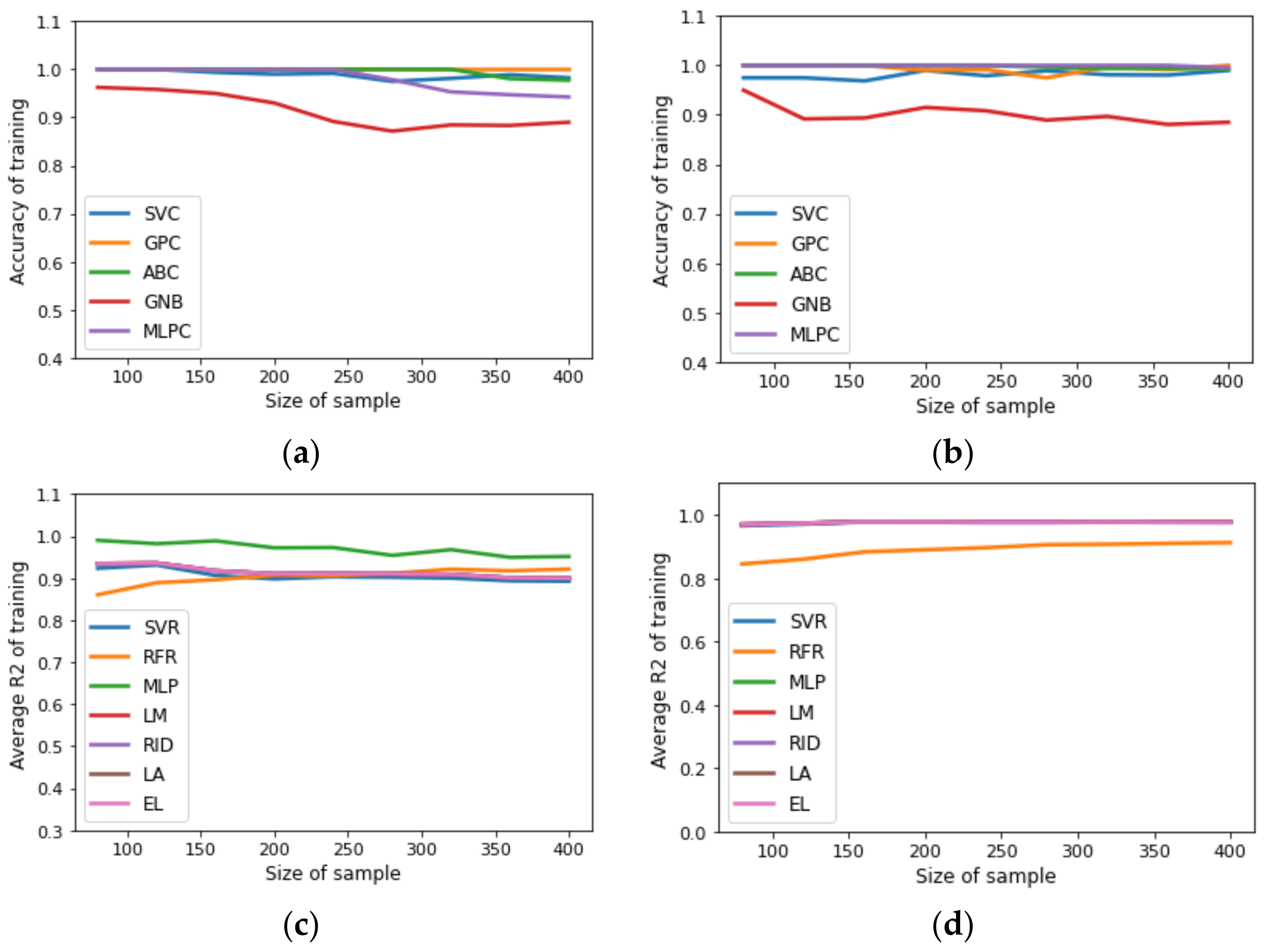
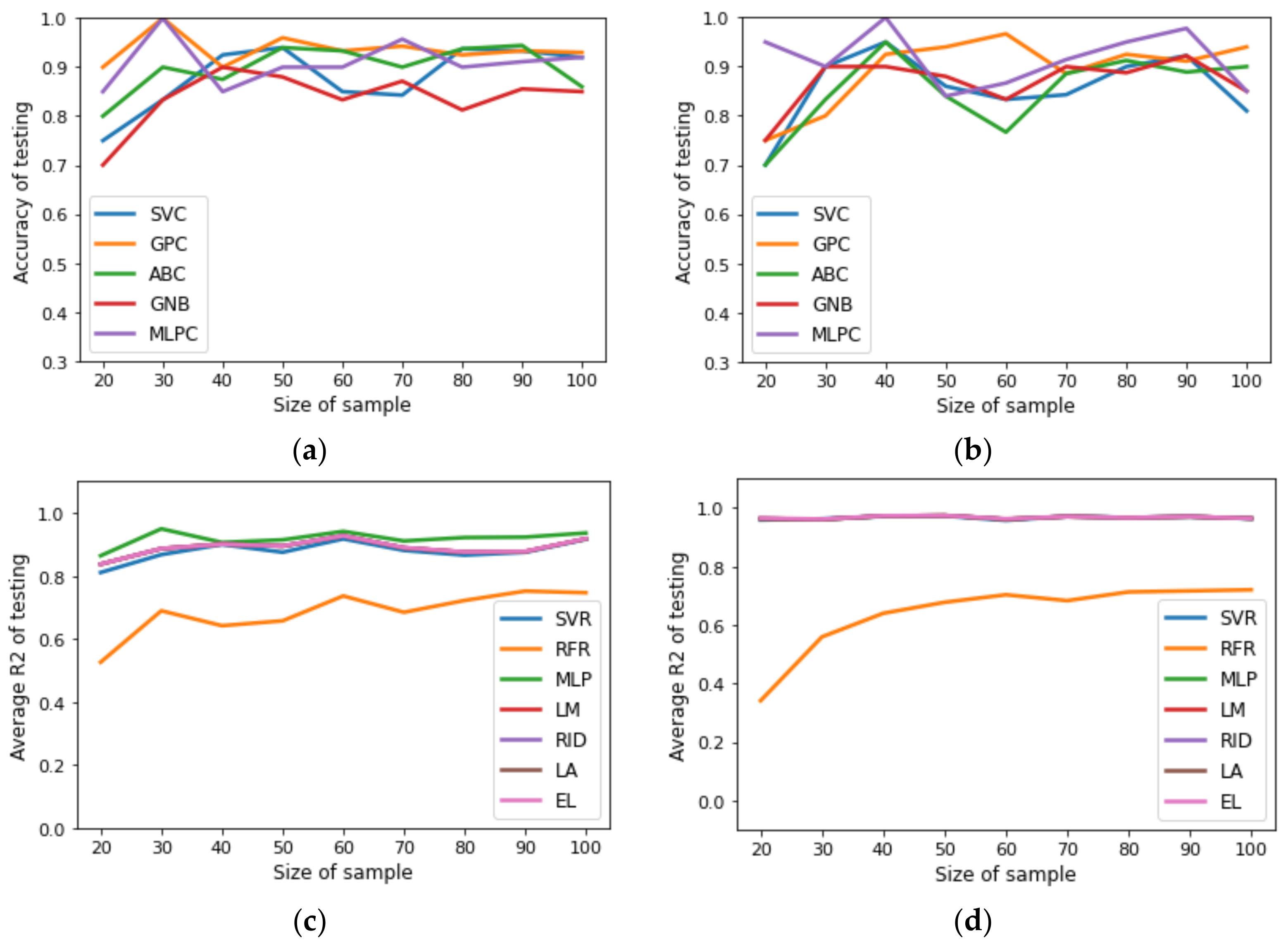
In order to study the effect of dataset size on the performance of surrogate models, the following procedure was implemented: first, the dataset (500 samples) obtained in the second stage of the methodology was sampled to generate sub-datasets of 100, 150, 200, 250, 300, 350, 400, 450, and 500 samples; second, the sub-datasets were divided into training datasets (80%) and testing datasets (20%); third, the training datasets were used to construct surrogate models and the testing datasets were used to identify overfitting surrogate models [30]. Figure 2 and Figure 3 reveal that the SML tools selected for the classification problems provided a good accuracy for predicting the structure of designed plants independent of dataset size, whereas the SML tools selected for regression, except RFR, provided a good average for predicting the metallurgical and profitability parameters of the designed plants independently of the dataset size. The accuracy of the classification was calculated via the confusion matrix, and the SML tool parameters were tuned via the trial-and-error method. The Supplementary Materials shows other performance measures, such as MSE, precision, and sensitivity. Based on the general parsimonious principle [31], LM and GPC surrogate models were selected for both scenarios. Next, the LM in each scenario was subjected to GSA using the Sobol–Jansen method. According to a related study [32], the size of sample needed to obtain reliable results with GSA must be equal to 30,000 and 40,000 for the first and second scenario, respectively; the results can be seen in Figure 4. The procedure implemented to select influential input variables considered two steps: first, ordering the normalized total indices from high to low; second, summing the normalized total indices until at least 0.90 of uncertainty on NPV was obtained. In the first scenario, copper price (1), cost of mine–crushing–grinding per ton of ore fed to the flotation plant (3), chalcopyrite fast mass flux fed (4), and chalcopyrite slow mass flux fed (5), were influential input variables on NPV (indices sum 0.9325), whereas in the second scenario, input variables (1,3,4,5) and the number of cells in the rougher (16), scavenger (19), and rescavenger (20) were influential input variables on NPV (indices sum 0.9226). Thus, in the first scenario, the uncertainty space was reduced from fifteen–dimensional to four–dimensional space, whereas for the second scenario, the uncertainty space was reduced from twenty–dimensional to seven–dimensional space. The execution time required to perform GSA was 230 s and 493 s for the first and second scenario, respectively. Note that applying GSA using the stochastic MINLP problem is infeasible due to the size of the sample and the execution time required to solve the deterministic MINLP.
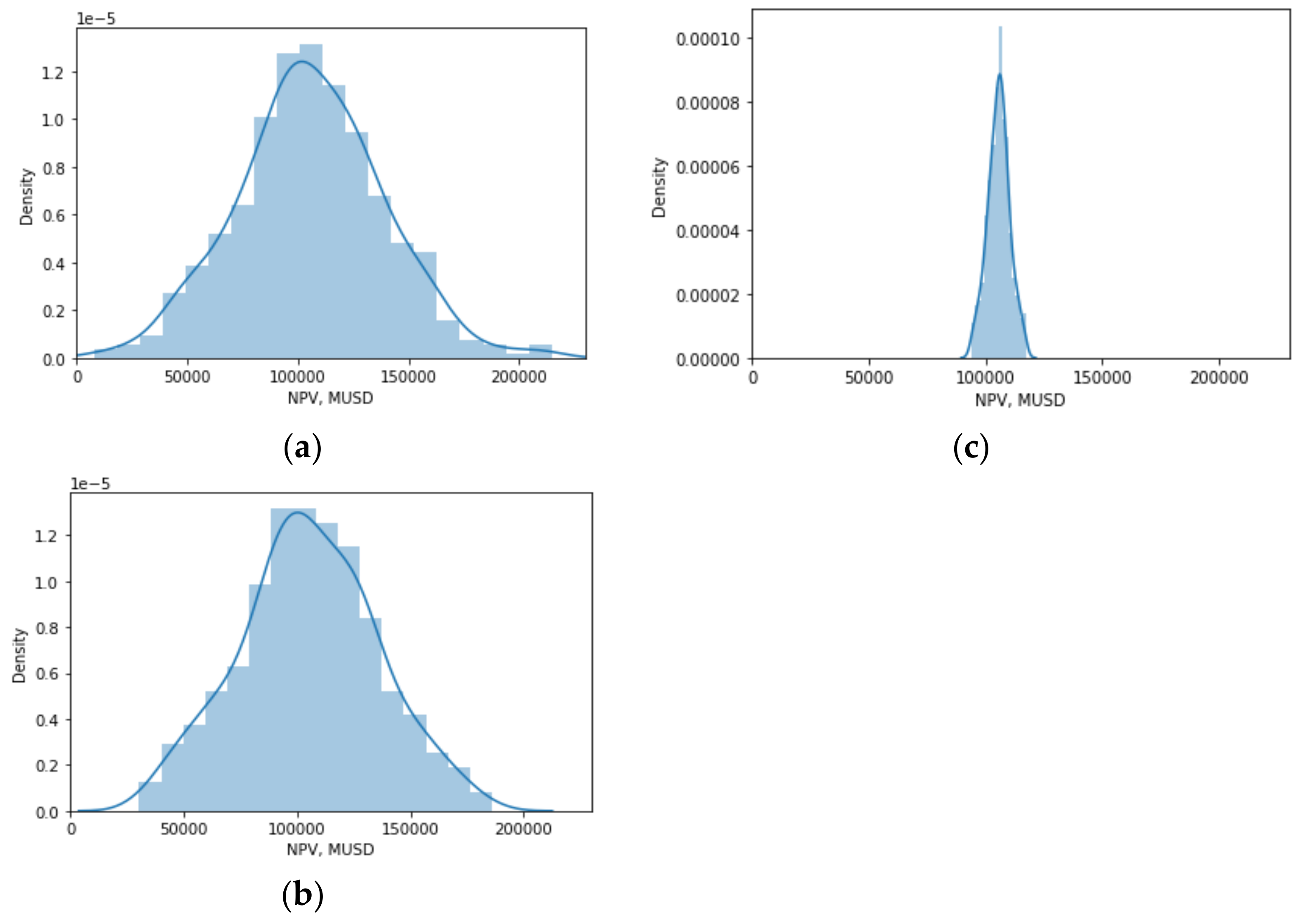
Next, the GSA results for the first scenario were checked. Specifically, the idea was to consider two groups, one formed by influential input variables and the other formed by noninfluential input variables, in order to analyze how the histogram of NPV is affected when the input variables of one or another group are fixed. Note that the NPV values were obtained via the BARON solver. Figure 5a shows the histogram of NPV when no groups are fixed. Figure 5b shows a histogram similar to the previous case, when the group of the noninfluential input variables were fixed on their standard operational conditions and we freed the influential group. Figure 5c shows a histogram distributed over a limited range, when we freed the noninfluential group and the group of influential input variables were fixed in their standard operational conditions. Therefore, the GSA results were confirmed. Figure 4 indicates that copper price and chalcopyrite flux fed are the main influential input variables on NPV for both scenarios and, consequently, on the structure, metallurgical parameters, and profitability parameters of the designed flotation plants. This could be attributed to the revenues generated by each flotation plant, which are a function of the copper price and copper mineralogical species present in the final concentrate, particularly chalcopyrite flux fed, the main copper species in porphyry–copper deposits located in northern Chile. The cost of mine–crushing–grinding per ton of ore fed to the flotation plant was the second most influential input variable on NPV for the first scenario, which could have been related to its effect on OPEX (see [27]), an aspect observed in industrial practice; in fact, mine–crushing–grinding costs represent around 60%–80% of the energy costs of mining projects [33,34]. The number of cells in the rougher, scavenger, and rescavenger were the second most influential input variables on NPV for the second scenario, which could have been related to their effect on CAPEX.
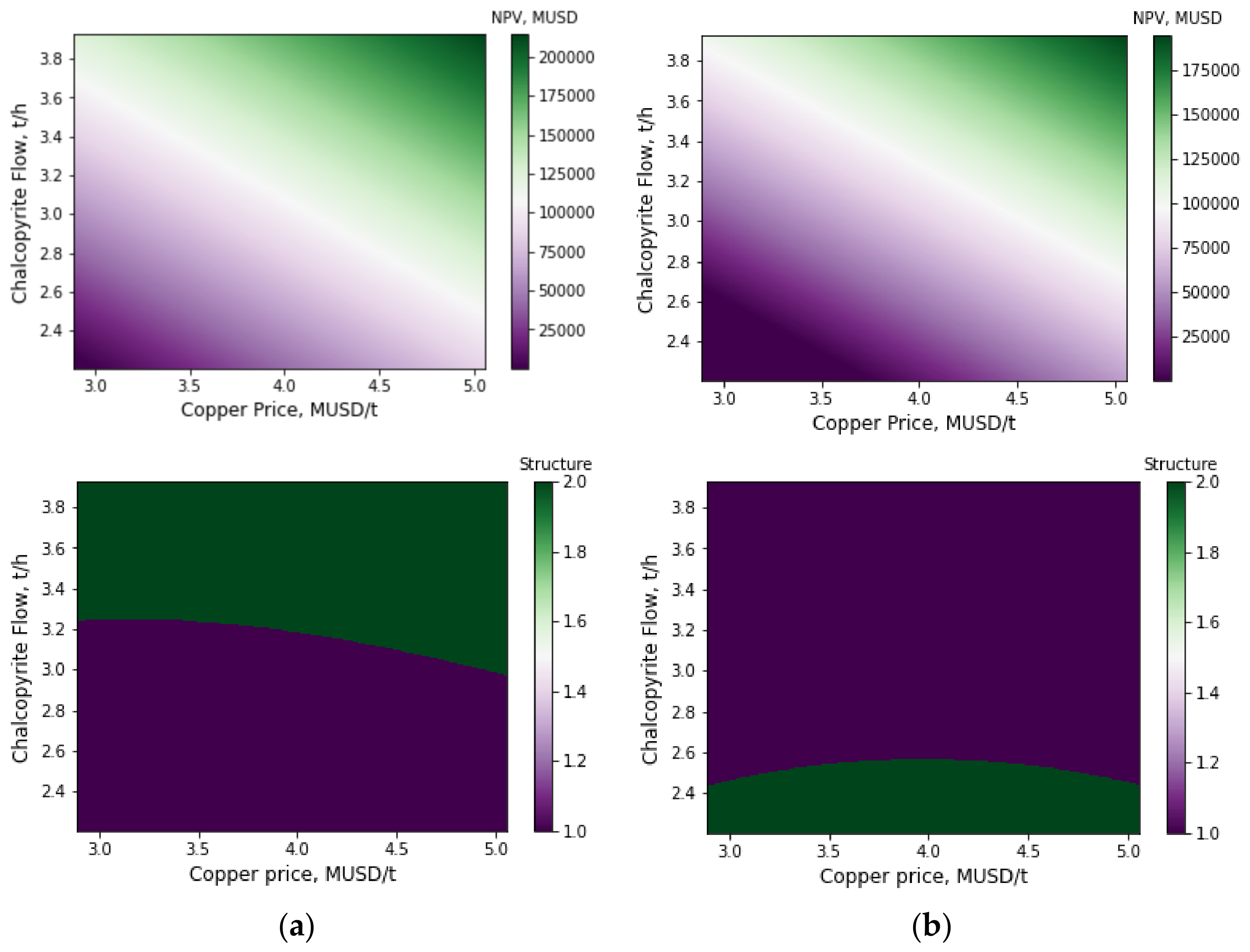
Surrogate models and information provided by GSA allowed us to visualize the behavior of NPV and the structure of designed plants in terms of copper price and chalcopyrite flux fed, as shown in Figure 6, where for the first scenario the rest of the input variables maintained standard values, whereas for the second scenario the number of cells in the rougher, scavenger, and rescavenger stages was seven and the rest of the input variables maintained standard values. In total, 160,000 estimations of surrogate models were required to produce these figures; the execution time was 210 s and 204 s for the first and second scenario, respectively. Obtaining similar results using the stochastic formulation is unfeasible due to the execution time required to solve the deterministic problems (approximately 26,496,000 s).
The stochastic optimization included the expectation minimization, the minimization of deviations from goals, the minimization of costs, and optimization over soft constraints; these objectives could be addressed partially via surrogate models because they could not predict: (a) the mineralogical species recoveries by the flotation stage; (b) the mass balance by mineralogical species in splitters, flotation stages, and mixers; (c) the number and volume of cells in each flotation stage; (d) the residence time by flotation stage; (e) the annual depreciation; (f) the working capital; and (g) the fixed capital costs, among others. A feasible alternative is to address the stochastic optimization problem via reduced formulation and approaches proposed in previous research, which is outside the focus of this work. However, some comments related to its application in mineral processing can be recorded: (a) Jamett et al., (2015) [7] implemented the two-stage stochastic programming to design flotation plants under uncertainty. This this approach optimized the expected total income over all the scenarios; such scenarios could be reduced to those derived from the influential input variables, allowing the analysis of scenarios relevant to total income and making efficient use of computational resources; (b) Liang et al., (2020) [8] implemented fuzzy mathematical programming to design flotation plants. This approach minimized the system uncertainty and maximized the expected profit over the uncertainty space formed by the fuzzification of the input variables; such space could be reduced to one formed only by the fuzzification of influential input variables, reducing the use of computational resources; (c) Cisternas et al., (2015) [10] and Acosta-Flores et al., (2020) [11] implemented the proof by exhaustion to study the effect of uncertainty on the flotation plant design; this approach involved a high RAM usage, especially when the problem was MINLP and the uncertainty space was large. The methodology proposed can be used to avoid the collapse of RAM.
4. Conclusions
The integration of supervised machine learning tools, global sensitivity analysis, and process design has been studied in previous research; however, its joint application in metallurgical process design has not been reported. Within this context, this work presented a methodology with which to reduce the size of the uncertainty space for stochastic optimization problems raised from design procedures, which includes four stages: stochastic optimization problems, the reduction of stochastic formulation to deterministic formulation and resolution using an exact algorithm, the construction of surrogate models using SML, and the submission of the surrogate models to GSA to determine input variables influential and noninfluential for optimization problem outcomes. The methodology was illustrated using a design procedure for flotation plants. Two scenarios were studied: in the first, the uncertainty space was reduced from fifteen-dimensional to four-dimensional space; in the second scenario, the uncertainty space was reduced from twenty-dimensional to seven-dimensional space. In addition, GSA information and surrogate models allow us to visualize relationships among influential input variables, which is unfeasible using the stochastic formulation. The methodology proposed could be used to improve the application of stochastic approaches in mineral processing design.
Supplementary Materials
The following are available online at https://www.mdpi.com/article/10.3390/min11121302/s1. Code: Scripts.
Funding
This research received no external funding.
Conflicts of Interest
The author declares no conflict of interest.
References
- Calisaya, D.A.; López-Valdivieso, A.; de la Cruz, M.H.; Gálvez, E.E.; Cisternas, L.A. A strategy for the identification of optimal flotation circuits. Miner. Eng. 2016, 96, 157–167. [Google Scholar] [CrossRef]
- Sassi, K.M.; Mujtaba, I.M. Effective design of reverse osmosis based desalination process considering wide range of salinity and seawater temperature. Desalination 2012, 306, 8–16. [Google Scholar] [CrossRef]
- Herrera-León, S.; Lucay, F.A.; Cisternas, L.A.; Kraslawski, A. Applying a multi-objective optimization approach in designing water supply systems for mining industries. The case of Chile. J. Clean. Prod. 2019, 210, 994–1004. [Google Scholar] [CrossRef]
- Hernández, I.F.; Ordóñez, J.I.; Robles, P.A.; Gálvez, E.D.; Cisternas, L.A. A Methodology for Design and Operation of Heap Leaching Systems. Miner. Process. Extr. Metall. Rev. 2017, 38, 180–192. [Google Scholar] [CrossRef]
- Gálvez, E.D.; Vega, C.A.; Swaney, R.E.; Cisternas, L.A. Design of solvent extraction circuit schemes. Hydrometallurgy 2004, 74, 19–38. [Google Scholar] [CrossRef]
- Sahinidis, N.V. Optimization under uncertainty: State-of-the-art and opportunities. In Computers and Chemical Engineering; Elsevier: Amsterdam, The Netherlands, 2004. [Google Scholar]
- Jamett, N.; Cisternas, L.A.; Vielma, J.P. Solution strategies to the stochastic design of mineral flotation plants. Chem. Eng. Sci. 2015, 134, 850–860. [Google Scholar] [CrossRef] [Green Version]
- Liang, Y.; He, D.; Su, X.; Wang, F. Fuzzy distributional robust optimization for flotation circuit configurations based on uncertainty theories. Miner. Eng. 2020, 156, 106433. [Google Scholar] [CrossRef]
- Liang, Y.; He, D.; Wang, Q.; Lu, X. Fuzzy distributional chance-constrained programming for handling stochastic and epistemic uncertainties during flotation processes. Chem. Eng. Res. Des. 2020, 164, 248–260. [Google Scholar] [CrossRef]
- Cisternas, L.A.; Jamett, N.; Gálvez, E.D. Approximate recovery values for each stage are sufficient to select the concentration circuit structures. Miner. Eng. 2015, 83, 175–184. [Google Scholar] [CrossRef]
- Acosta-Flores, R.; Lucay, F.A.; Gálvez, E.D.; Cisternas, L.A. The effect of regrinding on the design of flotation circuits. Miner. Eng. 2020, 156, 106524. [Google Scholar] [CrossRef]
- Lucay, F.; Mellado, M.E.; Cisternas, L.A.; Gálvez, E.D. Sensitivity analysis of separation circuits. Int. J. Miner. Process. 2012, 110–111, 30–45. [Google Scholar] [CrossRef]
- Sepúlveda, F.D.; Cisternas, L.A.; Gálvez, E.D. The use of global sensitivity analysis for improving processes: Applications to mineral processing. Comput. Chem. Eng. 2014, 66, 221–232. [Google Scholar] [CrossRef]
- Sutton, R.R.S. Generalization in Reinforcement Learning: Successful Examples Using Sparse Coarse Coding. In Advances in Neural Information Processing Systems 8; MIT Press: Cambridge, MA, USA, 1996; pp. 1038–1044. [Google Scholar]
- Vollmer, N.I.; Al, R.; Sin, G. Benchmarking of Surrogate Models for the Conceptual Process Design of Biorefineries. In Computer Aided Chemical Engineering; Elsevier: Amsterdam, The Netherlands, 2021; Volume 50, pp. 475–480. [Google Scholar]
- Pedrozo, H.A.; Rodriguez Reartes, S.B.; Chen, Q.; Diaz, M.S.; Grossmann, I.E. Surrogate-model based MILP for the optimal design of ethylene production from shale gas. Comput. Chem. Eng. 2020, 141, 107015. [Google Scholar] [CrossRef]
- Jones, M.; Forero-Hernandez, H.; Zubov, A.; Sarup, B.; Sin, G. Superstructure Optimization of Oleochemical Processes with Surrogate Models. In Computer Aided Chemical Engineering; Elsevier: Amsterdam, The Netherlands, 2018; Volume 44, pp. 277–282. [Google Scholar]
- Xia, Z.; Wang, S.; Zhou, L.; Dai, Y.; Dang, Y.; Ji, X. Surrogate-assisted optimization of refinery hydrogen networks with hydrogen sulfide removal. J. Clean. Prod. 2021, 310, 127477. [Google Scholar] [CrossRef]
- Ning, C.; You, F. Optimization under uncertainty in the era of big data and deep learning: When machine learning meets mathematical programming. Comput. Chem. Eng. 2019, 125, 434–448. [Google Scholar] [CrossRef] [Green Version]
- Azzi, S. Surrogate Modelig of Stochastic Simulators. Ph.D. Thesis, Institut Polytechnique de Paris, Palaiseau, France, 4 June 2020. [Google Scholar]
- Kim, S.H.; Boukouvala, F. Machine learning-based surrogate modeling for data-driven optimization: A comparison of subset selection for regression techniques. Optim. Lett. 2020, 14, 989–1010. [Google Scholar] [CrossRef]
- Asher, M.J.; Croke, B.F.W.; Jakeman, A.J.; Peeters, L.J.M. A review of surrogate models and their application to groundwater modeling. Water Resour. Res. 2015, 51, 5957–5973. [Google Scholar] [CrossRef]
- Sun, X.Y.; Gong, D.; Li, S. Classification and regression-based surrogate model-assisted interactive genetic algorithm with individual’s fuzzy fitness. In Proceedings of the 11th Annual Genetic and Evolutionary Computation Conference, GECCO-2009, Montreal, QC, Canada, 8–12 July 2009; pp. 907–914. [Google Scholar]
- Gianey, H.K.; Choudhary, R. Comprehensive Review on Supervised Machine Learning Algorithms. In Proceedings of the 2017 International Conference on Machine Learning and Data Science, MLDS 2017, Noida, India, 14–15 December 2017; Volume 2018, pp. 38–43. [Google Scholar]
- Saltelli, A. Making best use of model evaluations to compute sensitivity indices. Comput. Phys. Commun. 2002, 145, 280–297. [Google Scholar] [CrossRef]
- Lucay, F.A.; Cisternas, L.A.; Gálvez, E.D. An LS-SVM classifier based methodology for avoiding unwanted responses in processes under uncertainties. Comput. Chem. Eng. 2020, 138, 106860. [Google Scholar] [CrossRef]
- Cisternas, L.A.; Lucay, F.; Gálvez, E.D. Effect of the objective function in the design of concentration plants. Miner. Eng. 2014, 63, 16–24. [Google Scholar] [CrossRef]
- Yianatos, J.B.; Henríquez, F.D. Short-cut method for flotation rates modelling of industrial flotation banks. Miner. Eng. 2006, 19, 1336–1340. [Google Scholar] [CrossRef]
- Komer, B.; Bergstra, J.; Eliasmith, C. Hyperopt-Sklearn: Automatic Hyperparameter Configuration for Scikit-Learn. In Proceedings of the 13th Python in Science Conference, Austin, TX, USA, 6–12 July 2014; pp. 32–37. [Google Scholar]
- Bashir, D.; Montañez, G.D.; Sehra, S.; Segura, P.S.; Lauw, J. An Information-Theoretic Perspective on Overfitting and Underfitting. In Proceedings of the Lecture Notes in Computer Science (including subseries Lecture Notes in Artificial Intelligence and Lecture Notes in Bioinformatics), Chanberra, Australia, 29–30 November; pp. 347–358.
- Seasholtz, M.B.; Kowalski, B. The parsimony principle applied to multivariate calibration. Anal. Chim. Acta 1993, 277, 165–177. [Google Scholar] [CrossRef]
- Pianosi, F.; Beven, K.; Freer, J.; Hall, J.W.; Rougier, J.; Stephenson, D.B.; Wagener, T. Sensitivity analysis of environmental models: A systematic review with practical workflow. Environ. Model. Softw. 2016, 79, 214–232. [Google Scholar] [CrossRef]
- Ballantyne, G.R.; Powell, M.S.; Tiang, M. Proportion of energy attributable to comminution. In Proceedings of the 1th Australasian Institute of Mining and Metallurgy Mill Operator’s Conference, Hobart, Australia, 29–31 October 2012; pp. 25–30. [Google Scholar]
- Silva, M.; Casali, A. Modelling SAG milling power and specific energy consumption including the feed percentage of intermediate size particles. Miner. Eng. 2015, 70, 156–161. [Google Scholar] [CrossRef]
Figure 1.
Predominant structures in the first and second scenario, (a) Structure 1, (b) Structure 2.
Figure 1.
Predominant structures in the first and second scenario, (a) Structure 1, (b) Structure 2.

Figure 2.
Benchmarking of SML tools to predict structure of designed process: (a) accuracy of training for uncertainty space of fifteen input variables; (b) accuracy of training for uncertainty space of twenty input variables. Benchmarking of SML tools to predict NPV, CAPEX, OPEX, REV, PROF, NCF, copper recovery, and copper grade: (c) average of training for uncertainty space of fifteen input variables; (d) average of training for testing dataset for uncertainty space of twenty input variables.

Figure 3.
Benchmarking of SML tools to predict structure of designed process: (a) accuracy of testing for uncertainty space of fifteen input variables; (b) accuracy of testing for uncertainty space of twenty input variables. Benchmarking of SML tools to predict NPV, CAPEX, OPEX, REV, PROF, NCF, copper recovery, and copper grade: (c) average of testing for uncertainty space of fifteen input variables; (d) average of testing for testing dataset for uncertainty space of twenty input variables.

Figure 4.
Global sensitivity analysis for (a) first scenario, and (b) second scenario.

Figure 5.
NPV histogram: (a) free input variables, (b) free influential and fixed noninfluential input variables, (c) free non-influential and fixed influential input variables.
Figure 5.
NPV histogram: (a) free input variables, (b) free influential and fixed noninfluential input variables, (c) free non-influential and fixed influential input variables.

Figure 6.
Estimation with surrogate models of NPV and structure for designed flotation plants in terms of the function of copper price and chalcopyrite flux fed: (a) first scenario, (b) second scenario.
Figure 6.
Estimation with surrogate models of NPV and structure for designed flotation plants in terms of the function of copper price and chalcopyrite flux fed: (a) first scenario, (b) second scenario.


Table 1.
Input variables under uncertainty. represents a normal distribution, represents an uniform distribution.
Table 1.
Input variables under uncertainty. represents a normal distribution, represents an uniform distribution.
| Input Variable | Standard Condition | Uncertainty |
|---|---|---|
| Copper price (1) | 4 MUSD/t | [4,0.3] |
| Kilowatt-hours (2) | 0.0002 MUSD | [0.0002,0.00002] |
| Cost of mine-crushing-grinding per ton of ore fed to plant (3) | 0.003 MUSD/t | [0.003,0.0004] |
| Chalcopyrite fast mass flux fed (4) | 3 t/h, | [3,0.3] |
| Chalcopyrite slow mass flux fed (5) | 2 t/h | [2,0.3] |
| Chalcocite fast mass flux fed (6) | 1 t/h | [1,0.1] |
| Chalcocite slow mass flux fed (7) | 1 t/h | [0.4,0.04] |
| Pyrite fast mass flux fed (8) | 5 t/h | [5,0.2] |
| Pyrite slow mass flux fed (9) | 3.5 t/h | [3.5,0.3] |
| Quartz mass flux fed (10) | 150 t/h | [150,3] |
| Gangue mass flux fed (11) | 300 t/h | [300,3] |
| Chalcopyrite fast copper grade fed (12) | 34% | [0.34.0.01] |
| Chalcopyrite slow copper grade fed (13) | 25% | [0.25,0.01] |
| Chalcocite fast copper grade fed (14) | 18% | [0.18,0.01] |
| Chalcocite slow copper grade fed (15) | 10% | [0.1,0.01] |
| Number of cells in the rougher stage (16) | 5 | [3,10] |
| Number of cells in the cleaner stage (17) | 5 | [3,10] |
| Number of cells in the recleaner stage (18) | 5 | [3,10] |
| Number of cells in the scavenger stage (19) | 5 | [3,10] |
| Number of cells in the rescavenger stage (20) | 5 | [3,10] |
Publisher’s Note: MDPI stays neutral with regard to jurisdictional claims in published maps and institutional affiliations. |
© 2021 by the author. Licensee MDPI, Basel, Switzerland. This article is an open access article distributed under the terms and conditions of the Creative Commons Attribution (CC BY) license (https://creativecommons.org/licenses/by/4.0/).
Share and Cite
MDPI and ACS Style
Lucay, F.A. Reducing the Dimensions of the Stochastic Programming Problems of Metallurgical Design Procedures. Minerals 2021, 11, 1302. https://doi.org/10.3390/min11121302
AMA Style
Lucay FA. Reducing the Dimensions of the Stochastic Programming Problems of Metallurgical Design Procedures. Minerals. 2021; 11(12):1302. https://doi.org/10.3390/min11121302
Chicago/Turabian StyleLucay, Freddy A. 2021. "Reducing the Dimensions of the Stochastic Programming Problems of Metallurgical Design Procedures" Minerals 11, no. 12: 1302. https://doi.org/10.3390/min11121302
Note that from the first issue of 2016, this journal uses article numbers instead of page numbers. See further details here.