Importance of Spatial Autocorrelation in Machine Learning Modeling of Polymetallic Nodules, Model Uncertainty and Transferability at Local Scale

Abstract

Machine learning spatial modeling is used for mapping the distribution of deep-sea polymetallic nodules (PMN). However, the presence and influence of spatial autocorrelation (SAC) have not been extensively studied. SAC can provide information regarding the variable selection before modeling, and it results in erroneous validation performance when ignored. ML models are also problematic when applied in areas far away from the initial training locations, especially if the (new) area to be predicted covers another feature space. Here, we study the spatial distribution of PMN in a geomorphologically heterogeneous area of the Peru Basin, where SAC of PMN exists. The local Moran’s I analysis showed that there are areas with a significantly higher or lower number of PMN, associated with different backscatter values, aspect orientation, and seafloor geomorphological characteristics. A quantile regression forests (QRF) model is used using three cross-validation (CV) techniques (random-, spatial-, and cluster-blocking). We used the recently proposed “Area of Applicability” method to quantify the geographical areas where feature space extrapolation occurs. The results show that QRF predicts well in morphologically similar areas, with spatial block cross-validation being the least unbiased method. Conversely, random-CV overestimates the prediction performance. Under new conditions, the model transferability is reduced even on local scales, highlighting the need for spatial model-based dissimilarity analysis and transferability assessment in new areas.

1. Introduction

The spatial distribution of deep-sea polymetallic nodules (PMN) is currently of high interest due to their high metal content of Mn, Fe, Ni, Co, Cu, or Li. These metals are needed for green and decarbonized technologies, such as electric cars and wind turbines [1,2]. The European Union alone will need 60 times more lithium and 15 times more cobalt by 2050 than today [3] for this transition. Deep-sea resources such as PMN could support this transition, with predictive spatial mapping having a key role in mining-block prioritization.

PMN spatial mapping advanced by using autonomous underwater vehicles (AUVs) to acquire large volumes of hydroacoustic and image data allows for high-resolution seafloor reconstruction at meter and even down to centimeter scales. The quantitative analysis of images enlightens the PMN distribution, narrowing the spatial gap that arises from the sparse ground-truth box-corer samples (usually > 1.8 km) with very limited sampling area (0.25 m²) [4,5,6,7,8,9].

Multibeam echosounder (MBES) data (bathymetry and backscatter), seafloor lithology, environmental information (e.g., organic carbon content), and ground-truth information (photos, information from box-corer sampling) have been analyzed with machine learning (ML) methods, providing the spatial distribution of PMN [7,10,11,12,13,14,15]. However, the influence of spatial autocorrelation (SAC) on ML modeling has not been considered.

Spatial autocorrelation describes the phenomenon where local similarity (neighboring observations) is matched by value similarity (correlation between observations) [16]. When the examined variable is spatially autocorrelated, the assumption of independence among the observations in the cross-validation (CV) data is violated (i.e., the fitted model uses almost identical data for training and testing).

Recent studies in terrestrial and marine spatial ML modeling showed that if the commonly used, non-spatial, random k-fold CV is used, the prediction performance is over-optimistic when SAC exists in the data. The magnitude of the spatial overfitting varies based on the degree of SAC among the training points, the environmental similarity among the regions, and the ML method used [17,18,19,20,21,22,23,24,25]. In order to address the influence of SAC, different CV schemes have been proposed; the most common are buffer distances among training locations [18,26,27], successive distances [28], leaving one training location out [19,29], and spatial block training. Spatial blocks can be based on geographical coordinates clustering [30], latitudinal-blocking [23], systematic assignment, and environmental similarity clustering [17,23,31]. SAC also influences the ML feature selection methods and hyperparameter optimization, resulting in suboptimal variable selection and model parameters [19,25,29,32].

Applying ML models can also result in poor and unreliable predictions when they extrapolate in a new geographical area where the feature space varies [17,33,34,35]. Thus, there is a need for dissimilarity analysis between the training data and the new area the prediction should be performed for. Traditional non-spatial approaches, such as density plots and boxplots, can show the overall degree of differentiation but cannot identify where it occurs. Moreover, examining and interpreting such plots in multidimensional space is difficult and could lead to erroneous conclusions [36]. Spatial sample-based methods have been developed, relying on the univariate distribution range of each predictor and the new correlations among the predictors within their univariate distribution range [37,38,39,40]. Model-based methods have also been introduced, using the model weights and prediction error in the dissimilarity calculation [17,35,41].

This paper addresses the presence of SAC in the PMN distribution of a specific site and how this could influence the results in the various modelling steps of the ML workflow by studying:

(a) The use of SAC as source information for the feature selection before modeling. The proposed workflow uses the spatial clusters resulting from the local indicators of spatial association (LISA) and specifically from the local Moran’s I [16] and investigates their relations with the seafloor predictors using boxplots and the non-parametric Wilcoxon–Mann–Whitney test [42,43,44]. The Boruta algorithm [45] is used as an alternative automated ML method. Boruta is an all-relevant feature selection approach that has shown good performance in high and low-dimensional datasets [46,47,48]. It has been widely used in ML seafloor mapping studies, providing increased interpretability and prediction performance [48,49,50,51,52,53]. However, its performance under the presence of SAC has not been extensively investigated.

(b) The influence of SAC on the cross-validation workflow steps. Three techniques are studied: random k-fold CV, systematic spatial block, and feature space clustering. The latter two techniques were selected as they can highlight the biases due to SAC and environmental dissimilarity [17]. They are appropriate for big spatial data, as they require less computation time compared with other methods such as buffer distances [18].

(c) The random forests (RF) [54] spatial predictive uncertainty. The prediction uncertainty is an integral part of spatial modeling, as it provides an in-depth analysis of the prediction validity. It can also prioritize areas for future sampling; this is of interest particularly in deep-sea research, where available ground-truth data are typically scarce. The RF prediction uncertainty can be estimated with different methods [18]. Here, the quantile regression forests (QRF) [55] was selected, as studies showed that it could outperform other methods while it produces informative maps without the need for extensive data preprocessing and model assumptions [18,56,57,58,59].

(d) The recently proposed method of dissimilarity index and area of applicability (AOA) [35]. AOA can identify geographical areas with novel feature space conditions that could hinder a reliable model transfer.

To our current knowledge, this is the first time that these topics are investigated for a regression random forests model applied for predicting PMN spatial distribution. Moreover, the literature research yielded only two studies in the marine environment (habitat mapping) that consider and include spatial-CV or/and the AOA, highlighting the need for further investigation. Similarly, QRF has been applied only rarely for seafloor spatial predictive modeling, despite the popularity of the RF algorithm in general [60].

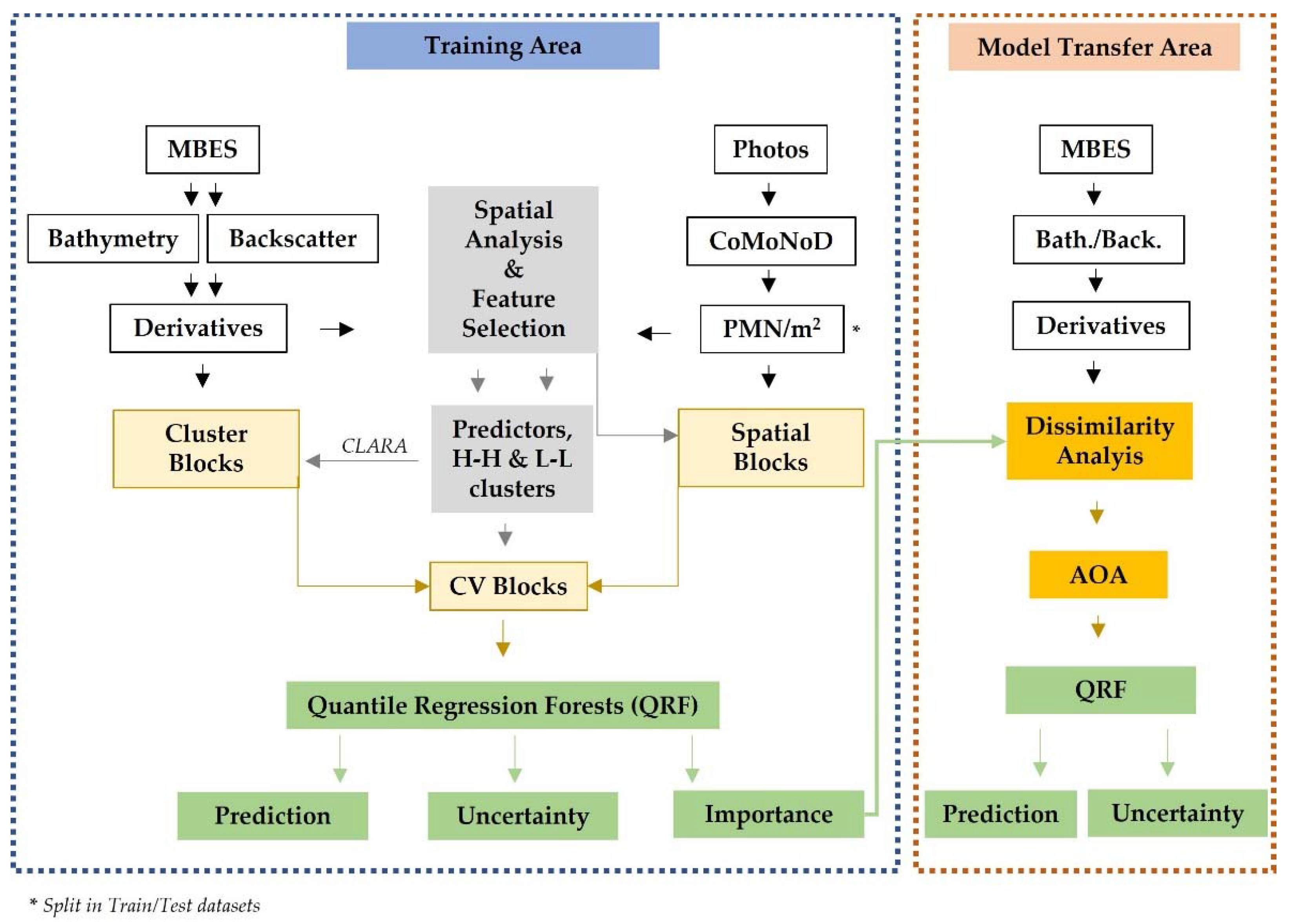
2. Materials and Methods

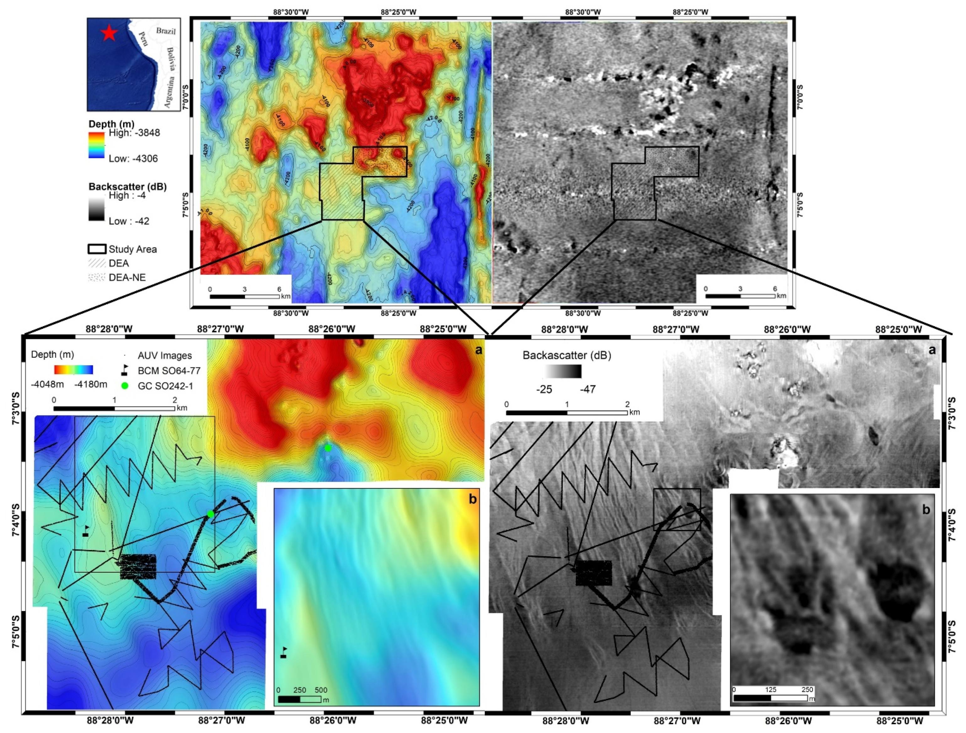
2.1. Study Area

The Peru Basin is one of the largest PMN fields globally, with an average abundance of 10 kg/m² [61]. Although the abundance and metal grade are of economic value [1], only a few studies have examined the PMN spatial distribution for economic reasons, focusing on the northern part of the investigated area that exhibits a substantial spatial variance [62,63,64,65]. In this northern part, lies the “DISturbance and reCOLonization” (DISCOL) experimental area (DEA). Inside the DEA (Figure 1), disturbance experiments were conducted to assess the environmental impact produced by a plough harrow [66,67]. The DEA is spatially heterogeneous regarding the seafloor morphology, geochemical properties, and PMN distribution, with many authors highlighting the need for further research [62,63,64,68,69]. The mapped area extends north and south of the DEA (in the N–S direction) and towards the northeast (hereafter DEA-NE). The entire region lies between −4047 m and −4179 m water depth, which is slightly above the regional carbonate compensation depth (CCD) at −4250 m [63]. The DEA itself has low relief, gentle slopes (<3°), longitudinal abyssal furrows, and areas with low reflectivity backscatter values and no PMN, hereafter called black patches (Figure 1). The sediments are layered clayey silts and silty clays, with foraminiferous residues and shell fragments [67,70].

The observed abyssal furrows strike perpendicularly to the regional contours and have a U-shape form. They are oriented parallel to the predominant NW bottom current flow [71,72]. Long-term studies showed that this deep flow is not stable but has periods of quasi-unidirectional strong currents (>5 cm/s but sometimes up to 17 cm/s) and periods with slower omnidirectional currents (1–3 cm/s). The recorded bottom current velocities are inside the velocity range that could preserve abyssal furrows [73]. The abyssal furrows act as bottom current channels, occasionally eroded during short periods of higher current velocities or even being relics from an earlier basin period, when the current regime was stronger [73,74,75]. Their preservation is supported by the low regional sedimentation rates of 0.4–2.0 cm/ka [76]. Past erosional bottom currents have also been proposed to be responsible for the formation of the black patches; these show Plio-Miocene carbonate-rich sediments as infilling [63,68,72].

The PMN-free black patches are easily recognizable due to their low backscatter reflectivity (Figure 1). They have an ellipsoid shape, with their long axes oriented downslope. Their depth varies between 2–5 m with remarkable flat and horizontal seafloors [67]. This downslope direction has been observed in other low reflectivity PMN-free patches in Peru Basin, connected with downslope sediment transport [68].

Larger-scale PMN-free areas with low backscatter reflectivity have also been observed for the Clarion-Clipperton Zone [15]. A recent gravity core inside a black patch in DEA (Figure 1) revealed that its geochemical conditions differ significantly from the surroundings, having increased organic carbon content (0.5 wt%–0.8 wt%) [69]. The increased organic carbon content might have shifted the Mn-redox closer to the seafloor, where the diagenetically mobilized Mn is released into the bottom water and thus not supporting the PMN formation [68,69,78,79]. Photos inside the black patch confirmed the absence of surficial PMN (Figure A1).

In the DEA-NE area, the seafloor is heterogeneous, with elongated and conical knolls and hills separated by local depressions. Visual inspection showed that the slopes have an extremely thin sediment coverage, while the local depressions act as sediment depocenters with increased sediment accumulation and talus debris [77]. The debris of basaltic fragments could act as nuclei supply to form new PMN [63,64]. PMN surficial coverage in this area varies, with black patches also present (Figure 1). The high-reflectivity sub-areas are mainly due to an exposed basement, such as the two 10 m high outcropping volcanic cones of pillow basalt inside a crate-shaped structure (Figure 1 and Figure A2). The visual inspection revealed the absence of sediments in their current-exposed, steep sides. PMN were found in the base of the crater, mixed with talus debris [67,77]. Geochemical analyses of the GC sediments revealed depth-profile variations for several chemical compounds, which exceed the area variability of other stations, highlighting the need for further research [69].

2.2. Hydroacoustic Data

High-resolution MBES data were acquired with the AUV Abyss from GEOMAR [80,81]. Bathymetric data processing was performed with the QPS Qimera 1.7 and MB-System 5.7 software (Monterey Bay Aquarium Research Institute (MBARI) University of New Hampshire and MARUM, Handelsweg, The Netherlands) [82]. The backscatter processing was carried out with QPS FMGT 7. The finally generated GeoTIFF grids have a 3 m × 3 m cell size, projected in Universal Transverse Mercator (UTM) zone 16S. Parts of the MBES data have been presented already by [67,83], but here they have been reprocessed and merged into one unified dataset.

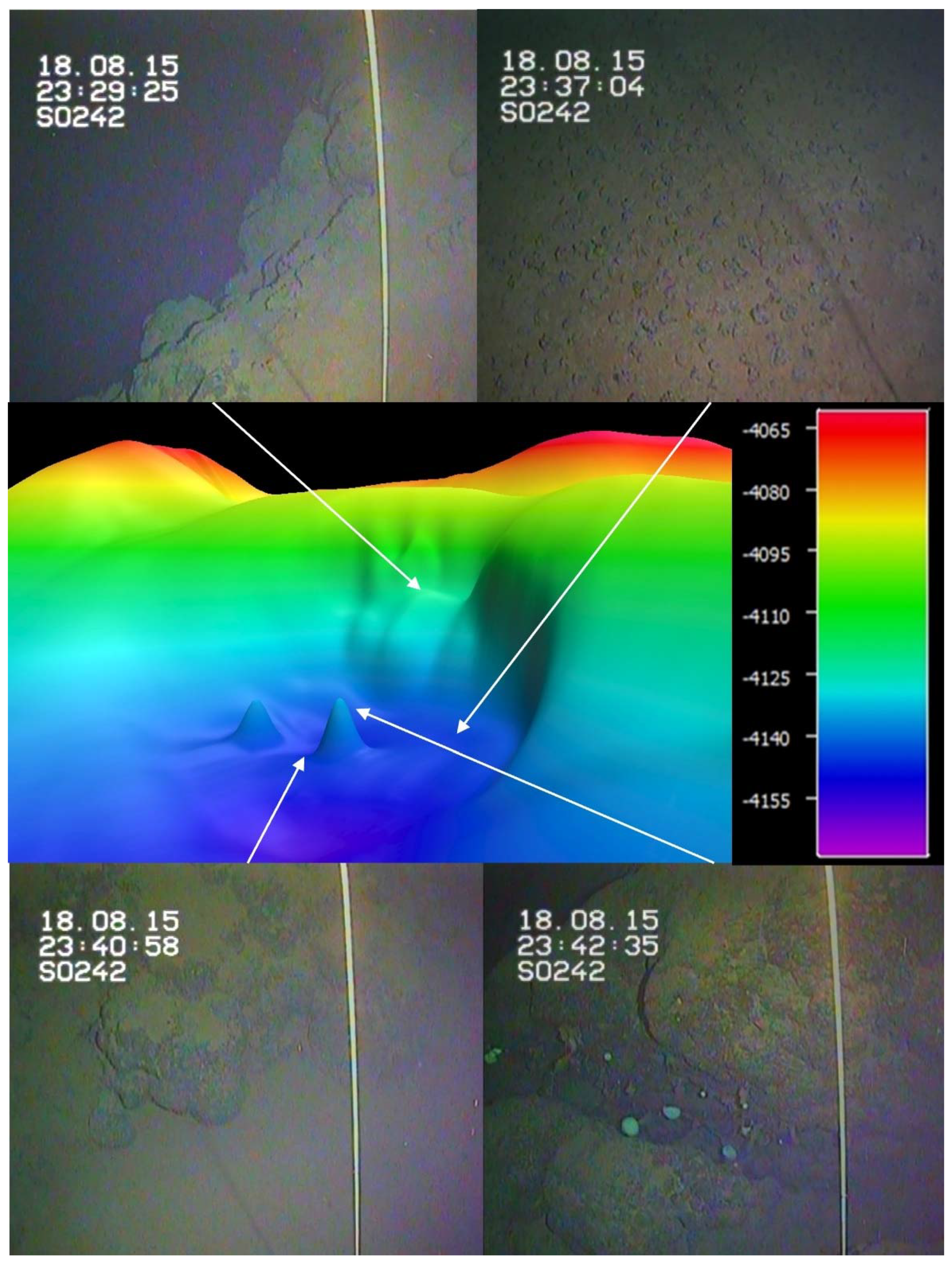
Seafloor Geomorphological Analysis

Sixteen derivatives of the bathymetric data were computed (

Table 1. MBES derivatives, their abbreviations, and references to their calculation algorithms.

MBES Derivatives	Abbreviation	Algorithm
Mean Depth	MD	Focal statistics *1
Deviation from Mean Depth	DFMD	Focal statistics *1
Slope	S	Zevenbergen and Thorne, 1987 *1 [95]
Northness	N	Olaya, 2009 *2 [96]
Eastness	E	Olaya, 2009 *2
Profile Curvature	PrC	Zevenbergen and Thorne, 1987 *1
Plan Curvature	PlC	Zevenbergen and Thorne, 1987 *1
Terrain Surface Convexity	TSC	Iwahashi and Pike, 2006 *1 [85]
Vector Ruggedness Measure	VRM	Sappington et al., 2007 *1 [97]
Bathymetric Position Index	BPI	Weiss, 2000 [98], Wilson et al., 2007 *1 [99]
Backscatter	BS	Focal statistics *1
Backscatter SD	BSSD	Focal statistics *1
Backscatter Local Moran	BSLM	Anselin, 1995 *3 [16]
Backscatter Entropy	BSE	Haralick et al. 1973 *4 [100]

*¹ SAGA GIS [101], *² Benthic Terrain Modeler [102], *³ raster package [103], *⁴ glcm package [104].

), following the recommendations of the current literature in the field of quantitatively geomorphometric analysis of seafloor data [50,84]. Derivatives were calculated based on a 10-cell (30 m) neighborhood, which is the minimum defined size for some of the derivatives (e.g., vector ruggedness measure) [85]. However, there are bathymetric derivatives that are calculated from a 3 × 3 cell neighborhood (e.g., slope, aspect). For those derivatives, the mean bathymetry was calculated first, and afterwards the derivative was determined. This approach shows better results than grid resampling or derivative averaging [86]. The 30 m neighborhood relates to the AUV positioning uncertainty, ensuring that the correct seafloor derivatives values will be extracted for each photo location. In this respect, a spatial autocorrelation of the predictors can further reduce the impact of positional uncertainty on the ML accuracy [87,88]. Moreover, the spatial autocorrelation could eliminate existing MBES artifacts that could affect the predictive modeling [52,89,90,91]. A multiscale approach was applied for the bathymetric position index, with finer and broader scales to better depict seafloor heterogeneity (0–30 m, 30–100 m, and 100–300 m). The aspect was transformed to northness and eastness [92,93,94]. Abbreviations and references to the algorithms of the calculated 14 derivatives are given in Table 1.

2.3. Optic Data

High-resolution photos were acquired by the deep survey camera system onboard the AUV Abyss [105]. The compact morphology-based nodule delineation (CoMoNoD) algorithm [9] was used for automated image analysis, providing the number of PMNs/m². CoMoNoD has been used for quantitative assessment and predictive modeling already [7,8], in which the advantages and limitations of the algorithm have been discussed.

We need to highlight that the primary goal of SO242-1 was to re-map in high-resolution the seafloor (acoustically and visually) inside and outside the DEA, which had been ploughed in 1989 [66,67], to have data that can provide insight into the current state of the environmental status and change when compared to previous data acquired between 1989 and 1996 [67,77]. Τhe crisscrossing AUV photo surveys were baseline exploration surveys about the general PMN occurrence and faunal distribution and were not meant to be a proper resource estimation survey. Generally, the optic data underestimate the number and abundance of PMN, and local correction factors (based on box-corer data from the photo locations) must be applied for a more realistic resource assessment [14,15,106,107,108,109].

For compiling the ground-truth dataset, all photos inside and next to the plough disturbance tracks were excluded, as they do not represent the original seafloor state [67]. The degree of blanketing around the tracks varies [67]. Nevertheless, the PMN abundance estimation in the area of the full coverage photomosaic (Figure 1) showed that the PMN could be effectively quantified, while it revealed the first signs of a correlation between PMN occurrence and seafloor morphology [9].

The optic data sampling in general has good geographical coverage (Figure 1), which is vital to efficiently depict the PMN spatial distribution trend, especially in local-scale studies such as ours [7,8,110]. The correlation points towards an underlying relationship between PMN and seafloor morphology that, synergistically with other environmental factors, influenced the PMN genesis and current spatial distribution. This is true, although the observed PMN number only represents the minimum number of nodules, as another part might occur within the sediment or due to a sediment cover that was not detected by the CoMoNoD algorithm.

In total, analyses of 30,000 photos were considered reliable and exported as ESRI shapefile in UTM 16S for further spatial analysis steps. The exported dataset was split into two independent datasets, creating the train and test dataset with 20,000 and 10,000 photos, respectively. The random data split without replacement was performed using the Subset Features tool (Geostatistical Analyst) in ArcMap 10.6 (© Environmental Systems Research Institute Inc. (ESRI), West Redlands, CA, USA); this tool ensures the same geographical coverage and statistical characteristics of the two generated datasets (Figure A3). The training dataset was used for the spatial autocorrelation analysis, feature selection, and spatial modeling, and the test dataset was used only for the final model evaluation. An overview of the different processing steps of the presented modelling workflow is given in Figure 2.

2.4. Spatial Data Analysis

The presence of spatial autocorrelation was investigated using the local indicators of spatial association (LISA) and particularly the local Moran’s I [16]. The local Moran’s I identifies clusters with significant spatial aggregation of similar high (H-H) or low (L-L) values (i.e., many or few PMN). The index was calculated using the Cluster and Outlier Analysis (Anselin Local Moran’s I) Tool (Spatial Statistics) in the ArcMap 10.6, according to the equations and null hypothesis provided as default from the software (i.e., the examined attribute is randomly distributed). The spatial relationship was based on the inverse Euclidian distance, and spatial weights were standardized to eliminate any bias that could be induced due to the uneven number of spatial neighbors. The analysis was based on 999 permutations. A false discovery rate correction was applied as the recommended approach to deal with the multiple testing and spatial dependency biases in large datasets; it provides significant clusters and outliers for a 95 per cent confidence level [111,112].

A visual boxplot analysis was performed between the two spatial clusters and their underlying MBES derivative values. In addition, the non-parametric Wilcoxon–Mann–Whitney [42,43,44] was used to identify significant differences in the MBES derivatives between the two spatial clusters. Due to the large sample size (inherent sampling variability), the substantive significance (effect size) was additionally used together with the statistical significance (p-value) for the interpretation of the results, when the p-values are similar or the same [113]. The base [114] and rstatix R packages were used here [115].

2.5. Feature Selection

The results from the spatial autocorrelation analysis were used jointly with the Boruta analysis for the feature selection. The Boruta algorithm creates a shuffled copy of each predictor variable and calculates the average variable importance using the ranger-RF algorithm [45]. The variables with higher importance than their shuffled copies are considered relevant to the target variable (PMN). Since all the relevant variables have been identified, Spearman’s rank correlation coefficient [116] was used to exclude correlated features with coefficient values > 0–5. Between two correlating features, the one with the higher relevance was kept. The Spearman correlation was preferred instead of, e.g., the Pearson correlation, as it is a non-parametric measure, which assesses the presence of monotonic relationships while being robust to outliers and deviations from normality [117,118]. For executing the features selection, the Boruta [45] and GGally [119] R packages were used.

2.6. Quantile Regression Forests

Random forests is an ensemble machine learning method designed of multiple classification or regression trees [54]. Each tree uses a random subset of the training data through bootstrapping. The remaining data (out-of-bag data) are used for internal error validation. Each tree node is split using the best subset of predictors randomly chosen, minimizing the correlation among trees. A tree is developed until the maximum depth is reached; the final predicted value of the regression results after averaging all trees predictions is finished. The QRF extends the random forests approach by keeping all the predicted values for each observation. This information assesses the conditional distribution and, thus, quantiles can be estimated. The range between the maximum and minimum quantile for a single prediction expresses the model uncertainty for this prediction. Here, the 0.05th and 0.95th quantiles were used for the lower and upper prediction uncertainty value.

RF performs well with the recommended default hyperparameter values (e.g., minimal node size, maximal tree depth) [7,48,120]. Nevertheless, the default caret [121] ranger-RF optimization process was applied, focusing on the number of variables available for splitting (mtry) and the splitting criterion. The permutation variable importance and the partial dependence plots (PDP) were also calculated using the pdp [122] R package. In a subpart of this study area, previous RF modelling showed an overall good prediction performance based on the internal OOB data [83].

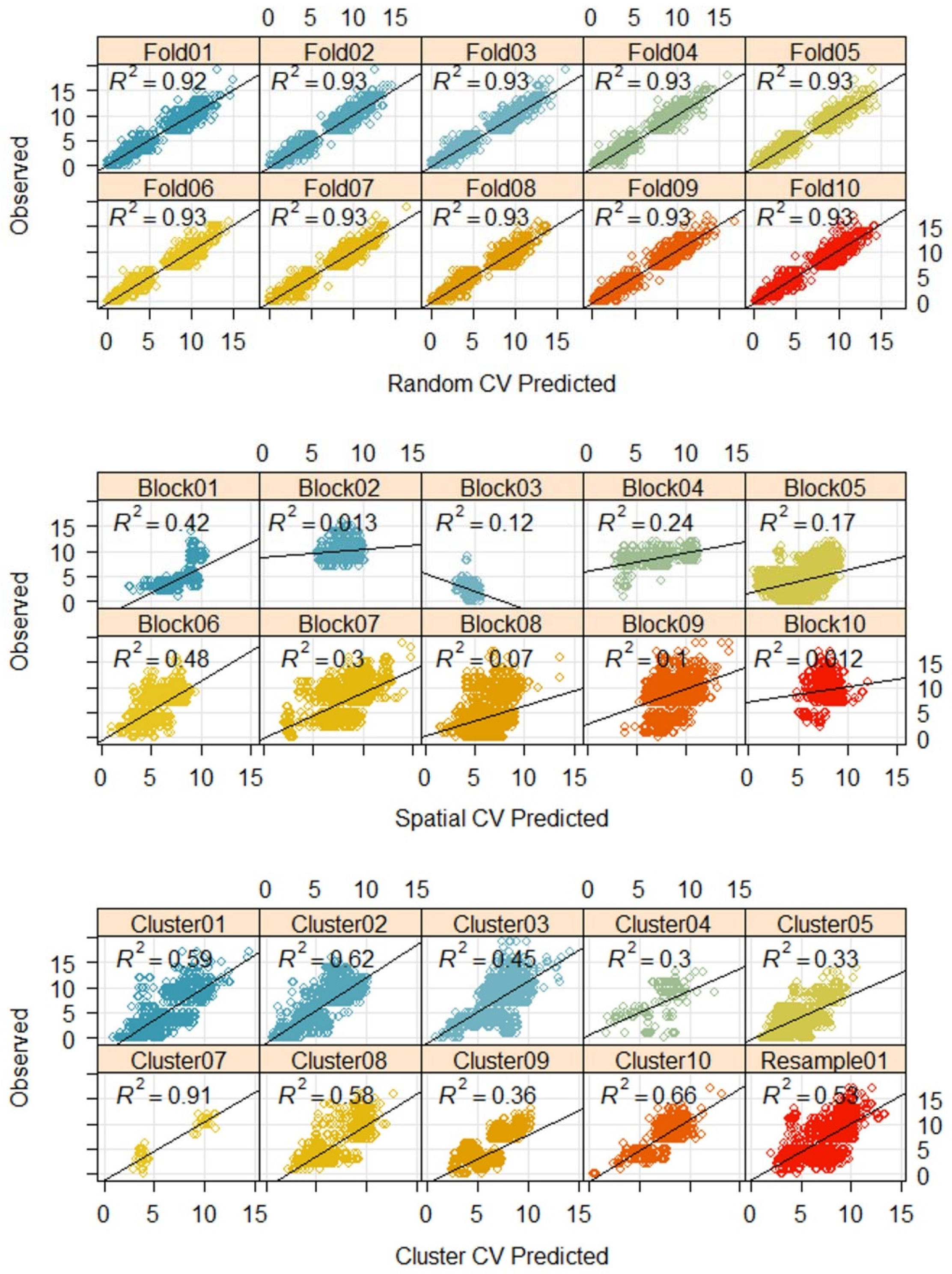
2.7. Cross-Validation Techniques

Three different cross-validation techniques have been tested.

2.7.1. Random k-fold Cross-Validation

Here, the model is repeatedly trained through random 10-fold CV, and its prediction performance is evaluated on the left-out fold data (k-1). Ten folds are recommended for large datasets, as they provide a good bias-variance trade-off [123].

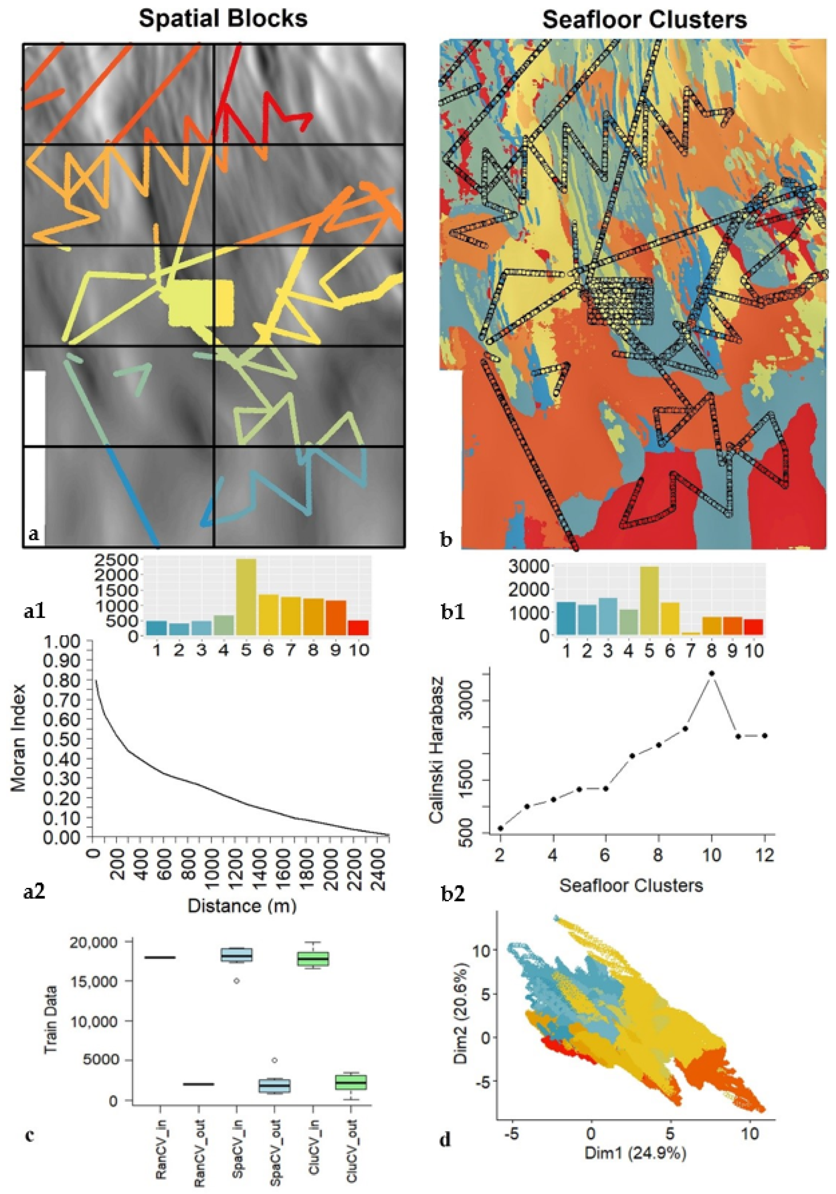
2.7.2. Systematic k-fold Spatial-Blocking Cross-Validation

Ten spatial non-overlapping folds (sub-areas) with equal geographical coverage (2 km × 1 km) were created using ArcMap 10.6 [Create Fishnet Tool (Data Management)] (Figure 3). The size of the block is a trade-off between the spatial autocorrelation range and the need for extrapolation [17,22,23,31]; it should minimize the influence of spatial autocorrelation in the training locations without creating extensive feature space differentiation among the blocks [17]. The Moran’s I incremental analysis [Incremental Spatial Autocorrelation Tool (Spatial Statistics)] showed that the spatial autocorrelation quickly drops after the 1st km (<0.25) and approaches almost zero (<0.05) from 2 km onward (Figure 3).

2.7.3. Feature Space k-fold Clustering Cross-Validation

As third method, the clustering large applications (CLARA) algorithm was used. CLARA [124] is a fast implementation of the partitioning around medoids [125] algorithm designed for large datasets. It uses an actual data point (medoid) as the center of each class, in which the sum of pairwise dissimilarities in this cluster is minimal; this method is robust to outliers. Only the predictors that resulted from the feature selection were clustered (Figure 3). The optimal number of clusters was based on the Calinski-Harabasz index [126]. The clustering was performed with the R packages cluster [127], clusterCrit [128], and RStoolbox [129].

It needs to be mentioned that both the random and the spatial k-fold CV can only be applied inside the DEA, where AUV footage exists and an objective comparison between the three CV techniques is possible. Nevertheless, it provides the opportunity for transferring the model to a different neighboring area, the DEA-NE. The spatial/cluster-blocking integration within the model training was performed with the CAST R package [130].

2.8. Dissimilarity Index and Area of Applicability

The recently proposed approach of using the dissimilarity index (DI) and area of applicability (AOA) [35] is a model-based method that assesses geographical areas, which have new feature space conditions and where the prediction error of a given pre-trained model exceeds the training CV error. The DI is based on the Euclidean feature space distances between the training dataset and the respective data of the new area. Before the distance calculation, predictors are scaled and weighted according to their variable importance of the model training. Thus, the distances of more important predictors account more to the DI estimation. The 0.95th quantile (outlier removed) of the DI is used as the AOA threshold. DI values between 0 and 1 indicate similar conditions, while values >1 indicate dissimilarity. Conversely, AOA values closer to 0 indicate unknown conditions for the extrapolation. The CAST R package was used.

3. Results

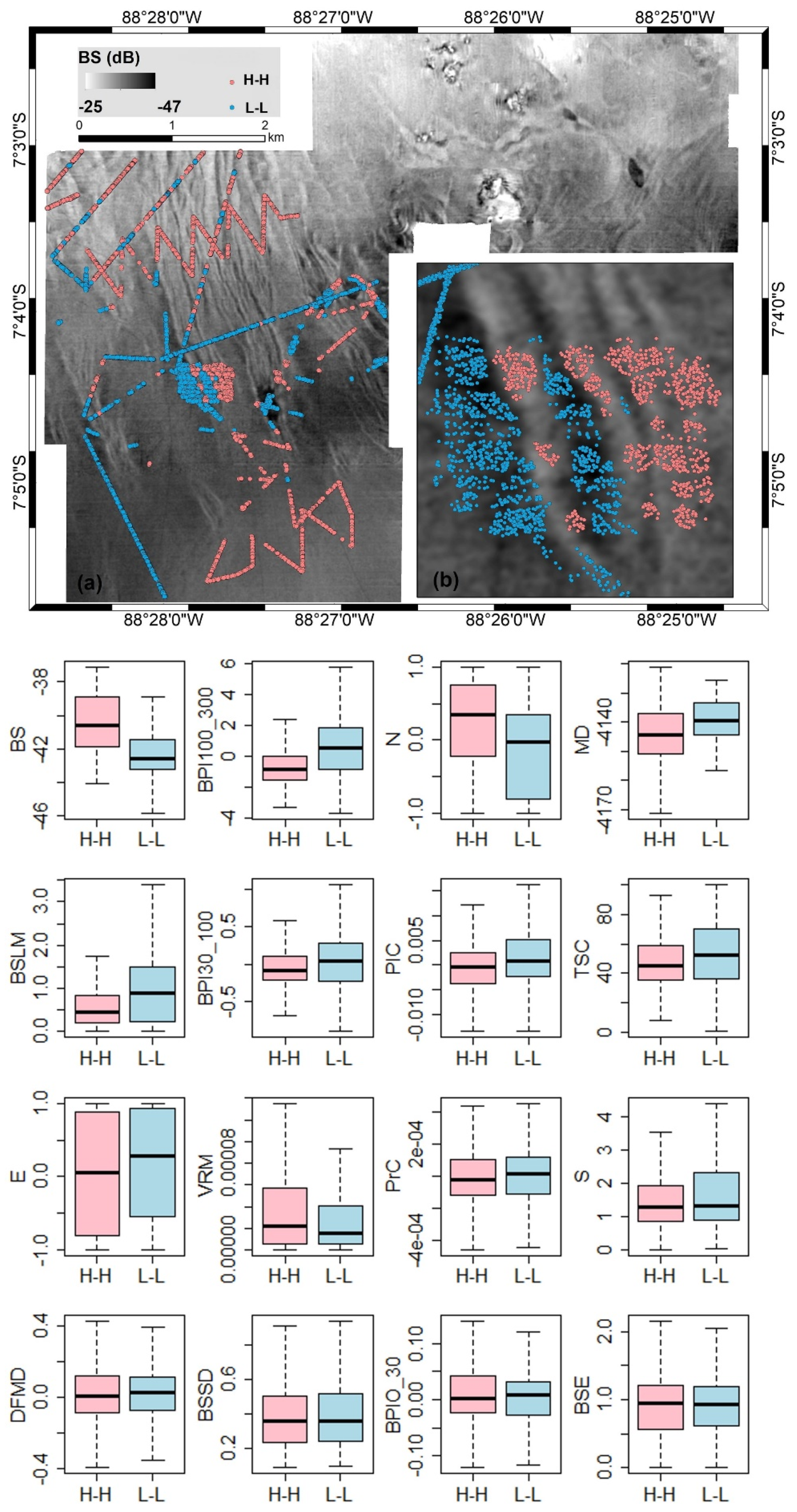
3.1. PMN Spatial Distribution and Spatial Autocorrelation

Plotting of the CoMoNoD results in a spatial context revealed a local scale heterogeneous PMN distribution, with higher numbers in the northeast and southwest parts of the studied area. Of particular interest is the central area within the photomosaic survey, where patches of high PMN numbers coexist next to areas with lower numbers. The PMN distribution follows the small-scale seafloor variations created by the abyssal furrows and the prevailing current regime (Figure A4). The local Moran’s I reveals that the majority of PMN (62%) are spatially aggregated into areas of H-H (27.5%) and L-L (34.5%) distributions (Figure 4). The boxplot analysis and the Wilcoxon–Mann–Whitney test show differences in the derivative distribution between the H-H and L-L clusters (Figure 4 and

Table 2. Wilcoxon–Mann–Whitney test results between statistically significant spatial clusters and MBES derivatives. The statistical significance (p-value) is given together with the substantive significance (effect size) for the interpretation of the results when the p-values are the same or similar. Its calculation and magnitude classification were based on [115].

Derivatives	Significance	Effect Size	Magnitude
Backscatter (BS)	p < 2.2 × 10−16	0.537	large
Bathymetric Position Index (BPI100_300)	p < 2.2 × 10−16	0.346	moderate
Northness (N)	p < 2.2 × 10−16	0.273	small
Mean Depth (MD)	p < 2.2 × 10−16	0.269	small
Backscatter Local Moran (BSLM)	p < 2.2 × 10−16	0.216	small
Bathymetric Position Index (BPI30_100)	p < 2.2 × 10−16	0.149	small
Plan Curvature (PlC)	p < 2.2 × 10−16	0.133	small
Terrain Surface Convexity (TSC)	p < 2.2 × 10−16	0.117	small
Eastness (E)	p < 2.2 × 10−16	0.077	small
Vector Ruggedness Measure (VRM)	p = 8.156 × 10−16	0.072	small
Profile Curvature (PrC)	p = 3.031 × 10−12	0.063	small
Slope (S)	p = 1.437 × 10−6	0.043	small
Deviation from Mean Depth (DFMD)	p = 0.00225	0.027	small
Backscatter SD (BSSD)	p = 0.04903	0.018	small
Bathymetric Position Index (BPI0_30)	p = 0.09455	0.015	small
Backscatter Entropy (BSE)	p = 0.64650	0.004	small

). In detail, higher BS values are linked with H-H clusters having a large effect in the test. The broad-scale BPI (100–300 m) also has significant differences between the two groups, with an observable moderate substantive significance (effect size). In contrast, the small-scale BPI (0–30 m) has no statistically significant variation between the two clusters. Similar to the backscatter entropy (BSE), the aspect of the seafloor surface plays a role in H-H clustering, as areas with higher numbers of PMN tend to be north-faced oriented (i.e., northness values closer to 1).

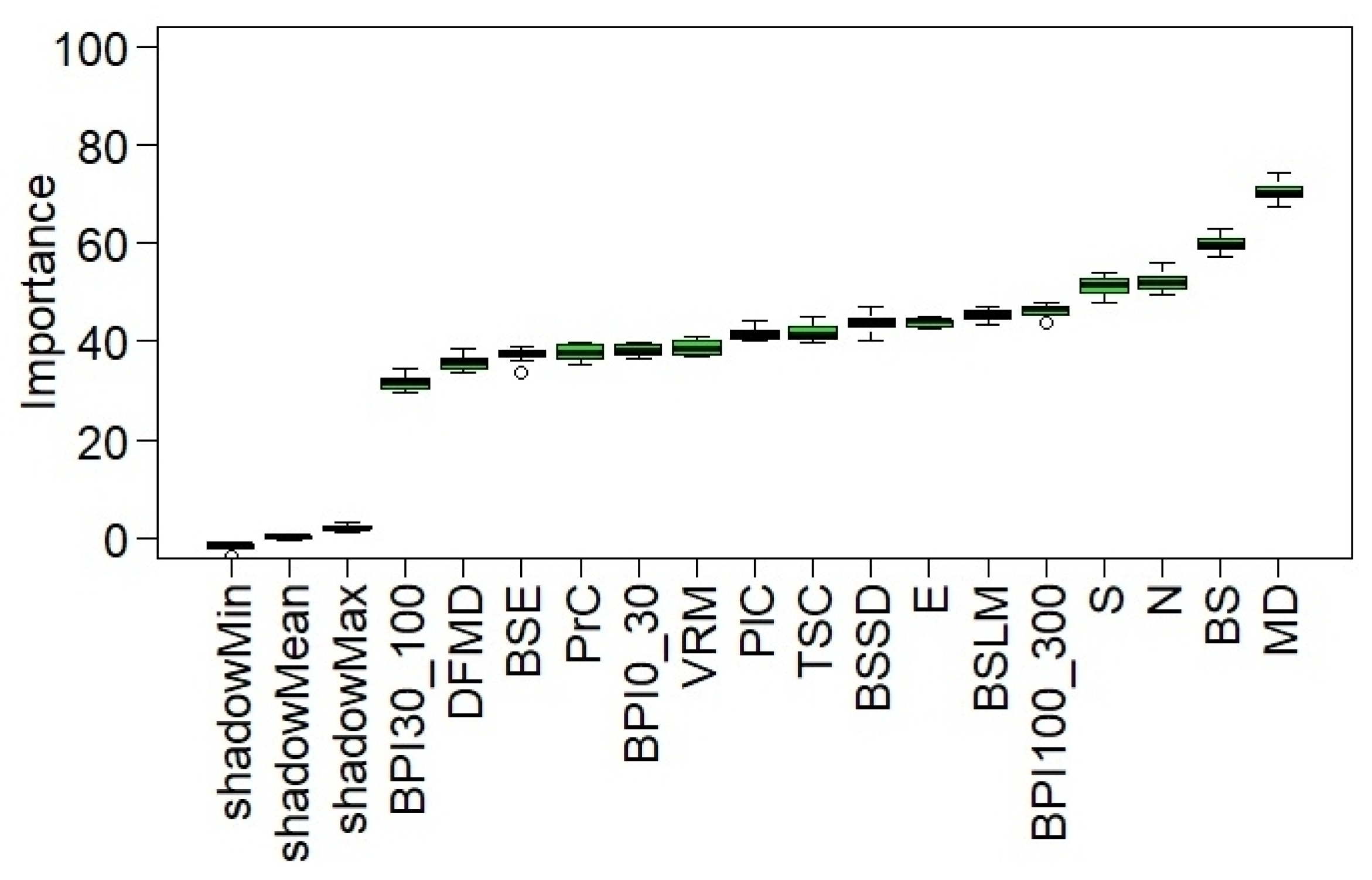
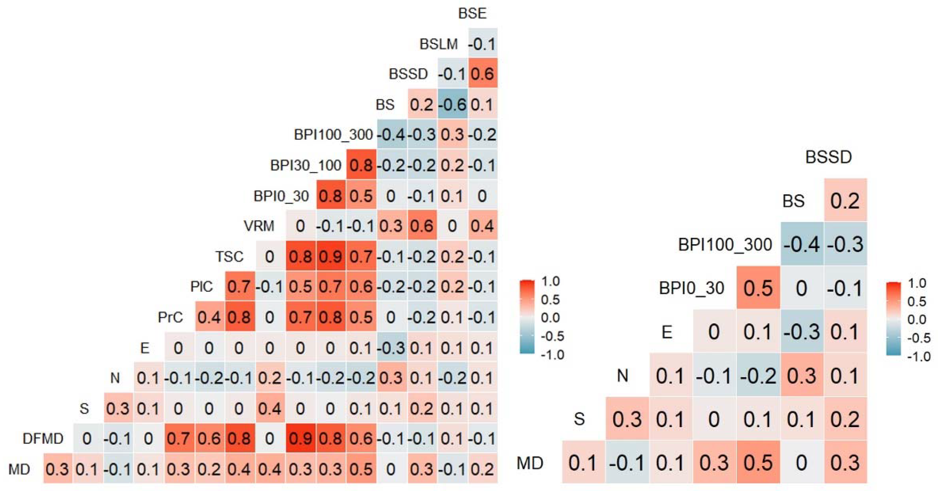
3.2. Boruta Analysis and Feature Selection

Similar to the spatial analysis, the Boruta algorithm shows that BS, BPI100_300, and northness are important and relevant predictors. However, the MD and not the BS is the most relevant predictor (Figure 5). Moreover, S and BSSD are ranked high, although both have not a significant difference between H-H and L-L groups (Table 2). Opposite to the Wilcoxon–Mann–Whitney test, Boruta results indicate that all derivatives are relevant to predict the PMN distribution. Using all variables leads to a highly correlated dataset (Figure A5) but excluding highly-correlated variables (r > ±0.5; in the Boruta importance score) results in the following predictors: MD, S, BS, N, BPI100_300, E, BSSD, and BPI0_30.

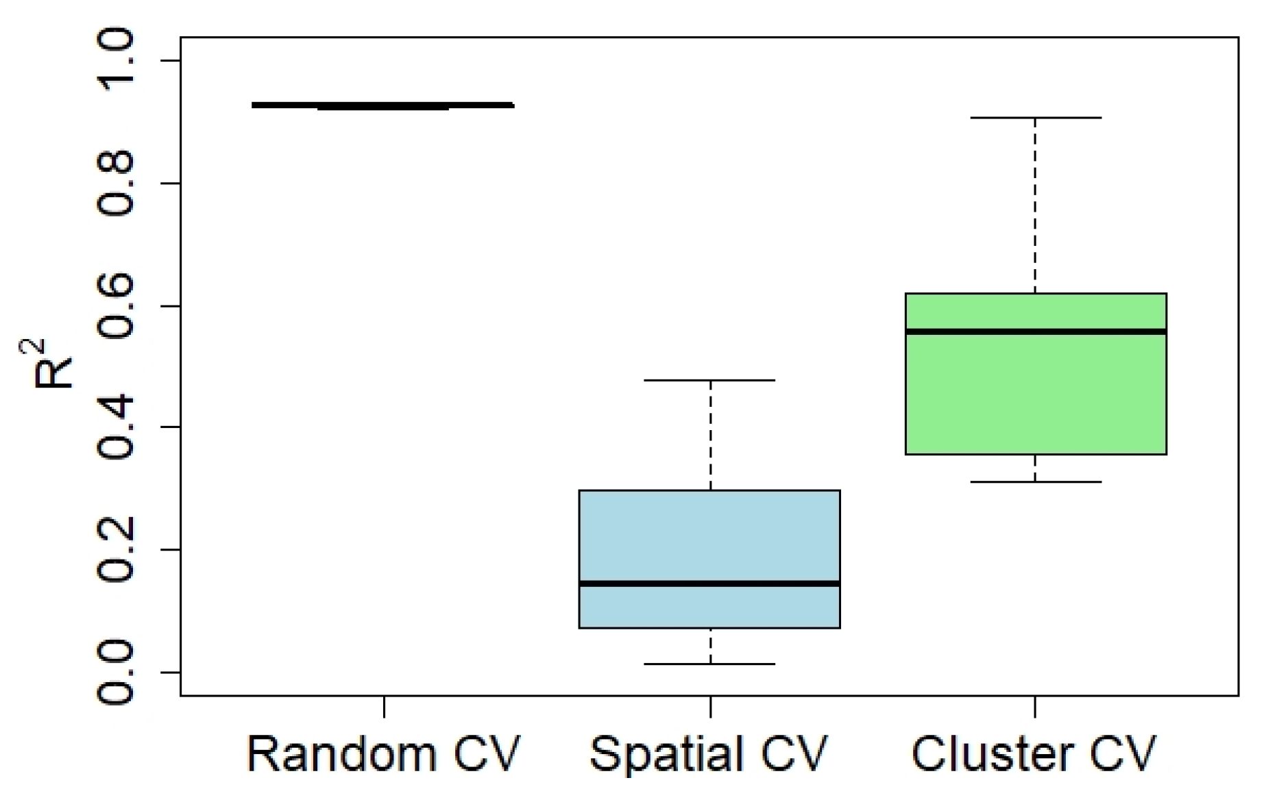
3.3. Model Training and CV Results

Based on the random-CV assessment, the QRF prediction performance was R² = 0.93. The same performance also results from the RF internal OOB error. However, when the spatial- and cluster-CV schemes were used, the prediction performance was reduced to R² = 0.19 and R² = 0.53, respectively (

Table 3. QRF performance (R²) for the three different CV schemes. The internal RF OBB error assessment is also provided.

Training Data	OOB	Random-CV	Spatial-CV	Cluster-CV
H-H and L-L data (12,327)	0.93	0.93	0.19	0.53
All training data (19,952)	0.87	0.87	0.14	0.46

). The performance is minimized when the spatial-blocking CV is applied. This shows that the model cannot efficiently transfer the predictions towards spatial blocks, where the SAC is low/absent and feature space extrapolation occurs to different degrees (Figure A6). The effect of feature space extrapolation is also depicted in the clustering CV error assessment. Here, in every training repetition, the model is trying to predict a new feature space cluster. This feature space can be completely new, or it has overlap with other clusters to a varying degree (Figure 3). This fact combined with the varying degree of spatial distance among the training points (and consequently varying SAC) results in a higher training error variance than spatial- and random-CV (Figure 6). The random-CV has a minimum training error variance due to the almost identical spatial and feature space characteristics of the randomly resampling folders. The performance analysis of each spatial/cluster block could provide in-depth information regarding the specific areas and seafloor clusters for which the model performs worst, potentially guiding future sampling (Figure A7).

The RF hyperparameter optimization differs between the spatial/cluster and random CV. In spatial- and cluster-CV, the optimum mtry value is eight (8), whereas it is five (5) in random-CV. This difference might result from the increased difficulty the model faces in spatial- and cluster-CV to extrapolate the predictions; it uses all the available information to gain predictive knowledge. In random-CV, the validation hold-out samples are identical to the training samples. Consequently, the model can predict well using fewer predictors.

3.3.1. Model Training and Sample Size

No significant correlation was found between the number of training samples used from the hold-in data and the prediction performance in the remaining (k-1) hold-out data (random-CV: −0.03 p = 0.93; spatial-CV: −0.11 p = 0.75; cluster-CV: 0.23 p = 0.51). The inclusion of all the available training points did not further improve the modeling performance, but resulted in a decrease, particularly in spatial- and cluster-CV (Table 3). This decrement is attributed to the noise added to the model by using the additional 38% of data that are not spatially aggregated. This ‘noise’ could be the result of the inherent natural variability of PMN distribution and/or wrong analyses of the CoMoNoD algorithm, e.g., through noise or lower resolution image data (greater distance to the seafloor).

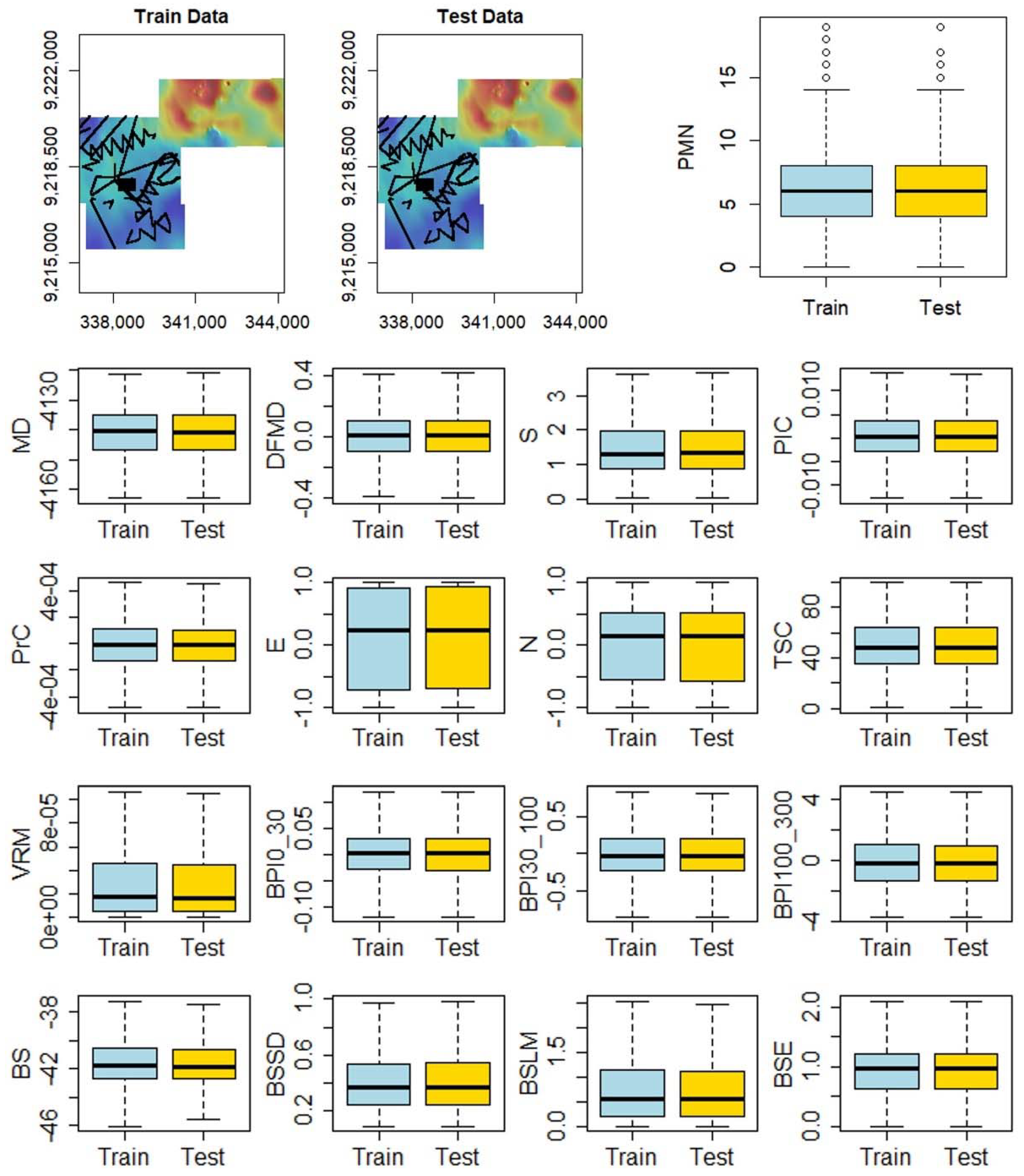
3.3.2. Model Performance in Test Data

The performance for the test data is the same for the three models (R² = 0.76), independently of the CV scheme followed. The higher predictive performance during the random-CV implies that data overfitting occurred. This is not the case for the spatial- and cluster-CV. At the end of the training cycle, the model has seen the same training data from the random folds, spatial blocks, and clusters and similar weights and relationships between predictors and response variables are established. The relationship type (e.g., monotonic, complex) and the marginal effect on the response variable are depicted as PDP in Figure 7 and Figure A8, Figure A9, Figure A10. The low-correlated dataset ensures that the assumption of independence (uncorrelated predictors) holds, and the PDP calculation is not violated [131,132].

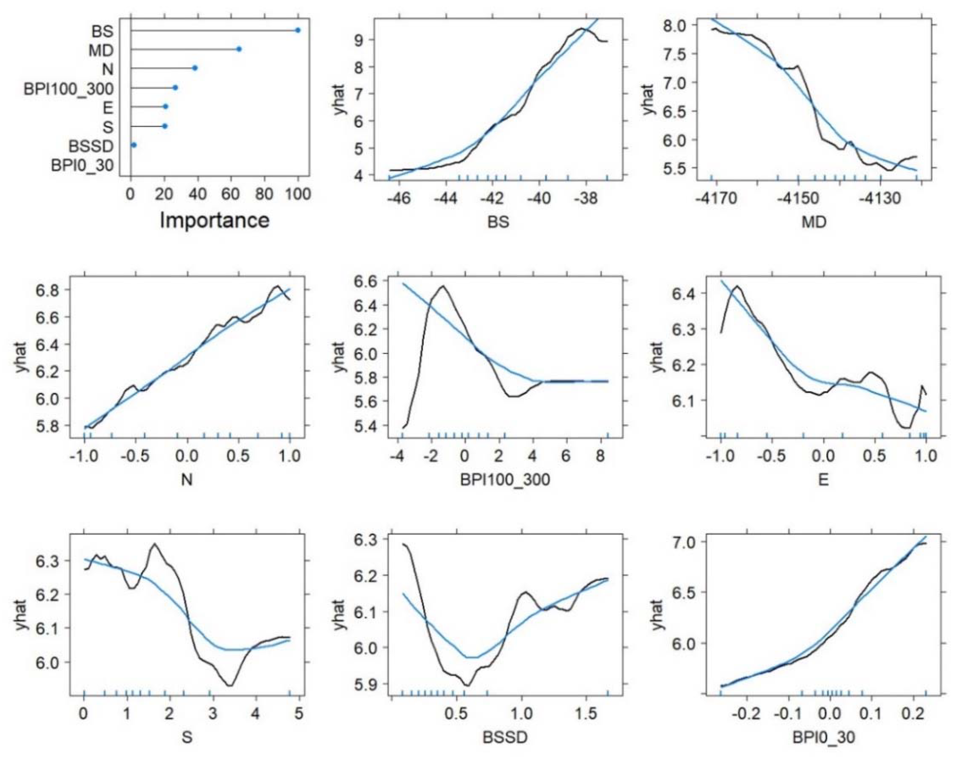
3.3.3. QRF Variable Importance

The backscatter (BS) has the highest variable importance, followed by mean depth (MD), northness (N), and the coarse bathymetric position index (BPI100_300). Slope (S) and eastness (E) contribute less, while the backscatter standard deviation (BSSD) and BPI0_30 have marginal or no contribution at all (Figure 7). This ranking is closer to the spatial analysis results than from the Boruta analyses, where the BSSD, S, and MD have scored higher. The overall higher agreement between local Moran’s I analysis and a spatially trained QRF shows that the Boruta may result in sub-optimum importance ranking, due to the overfitting that occurs when non-spatial training is performed.

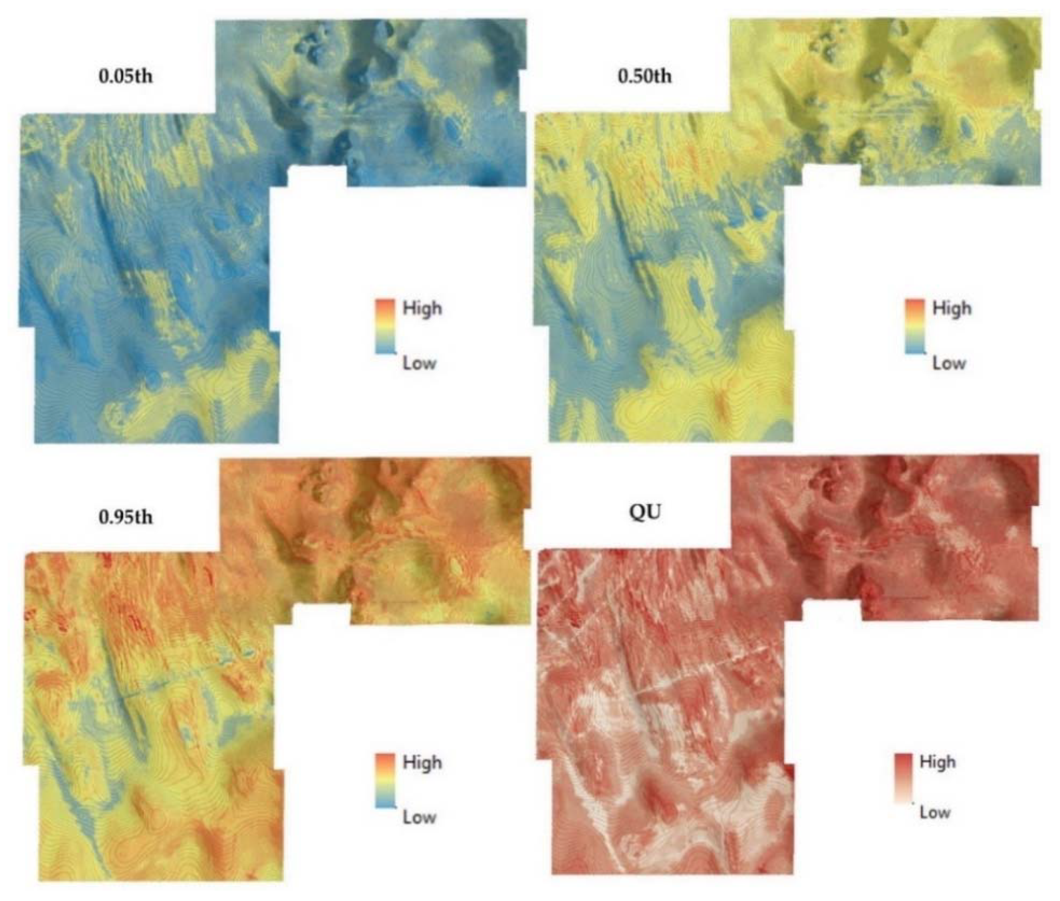
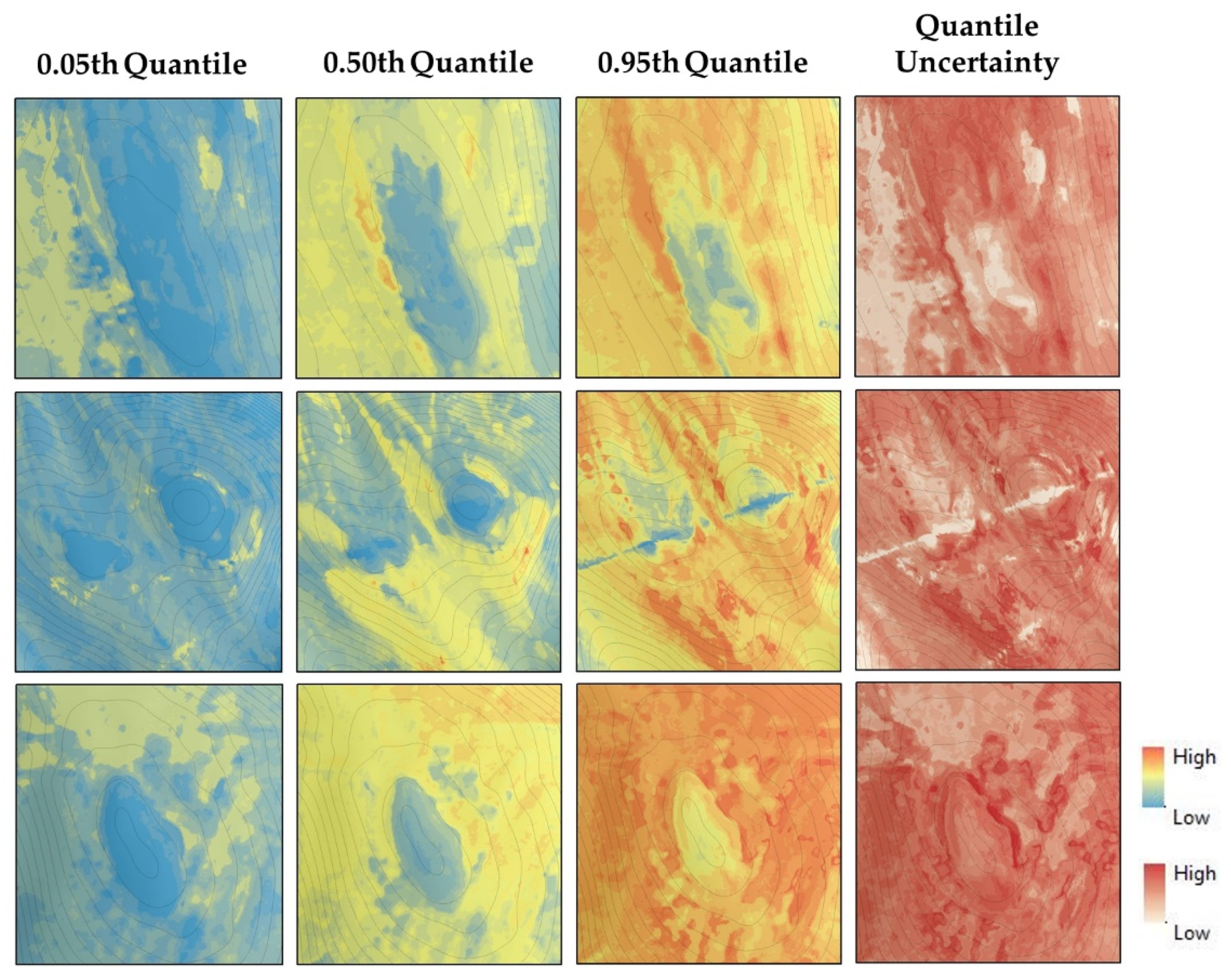
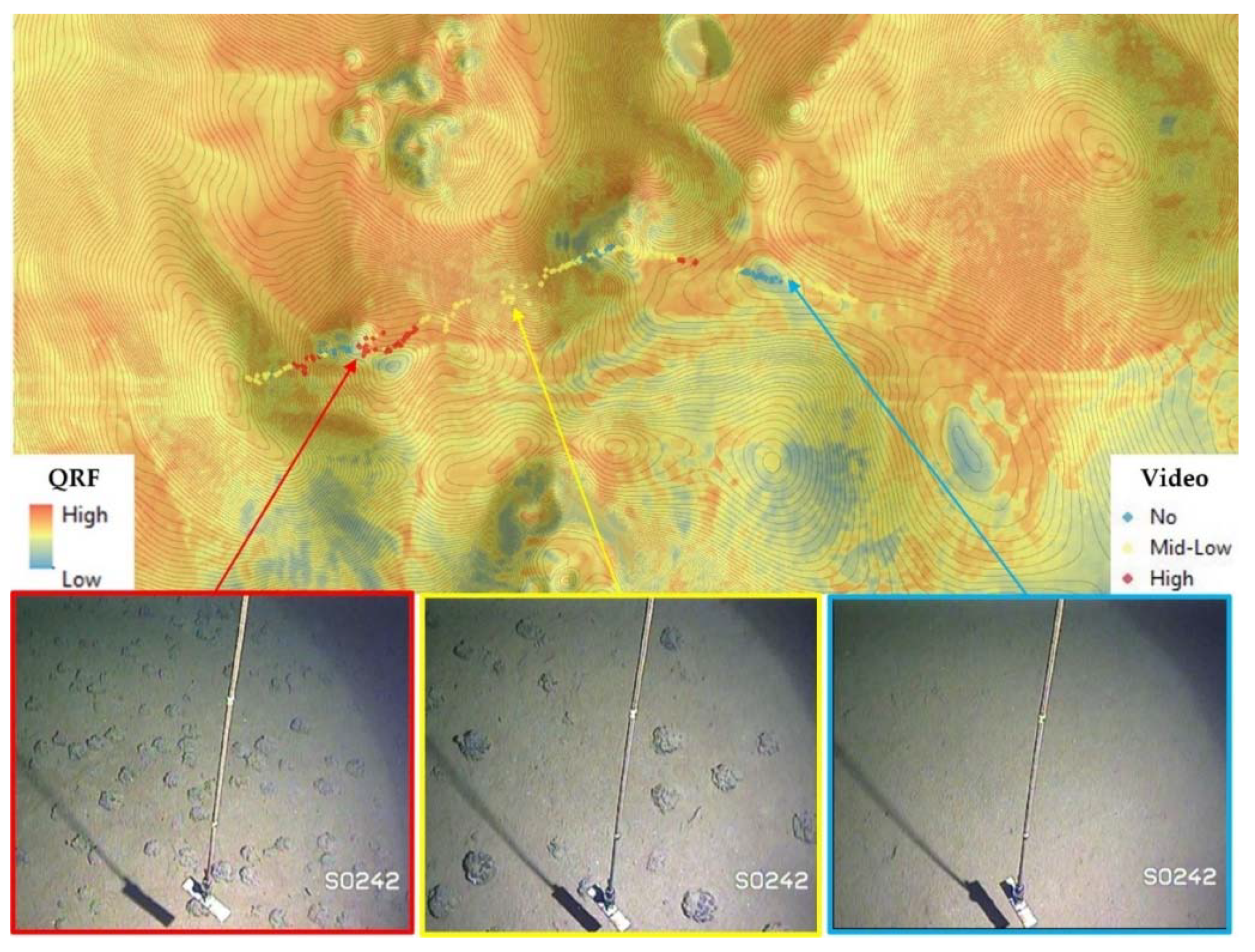
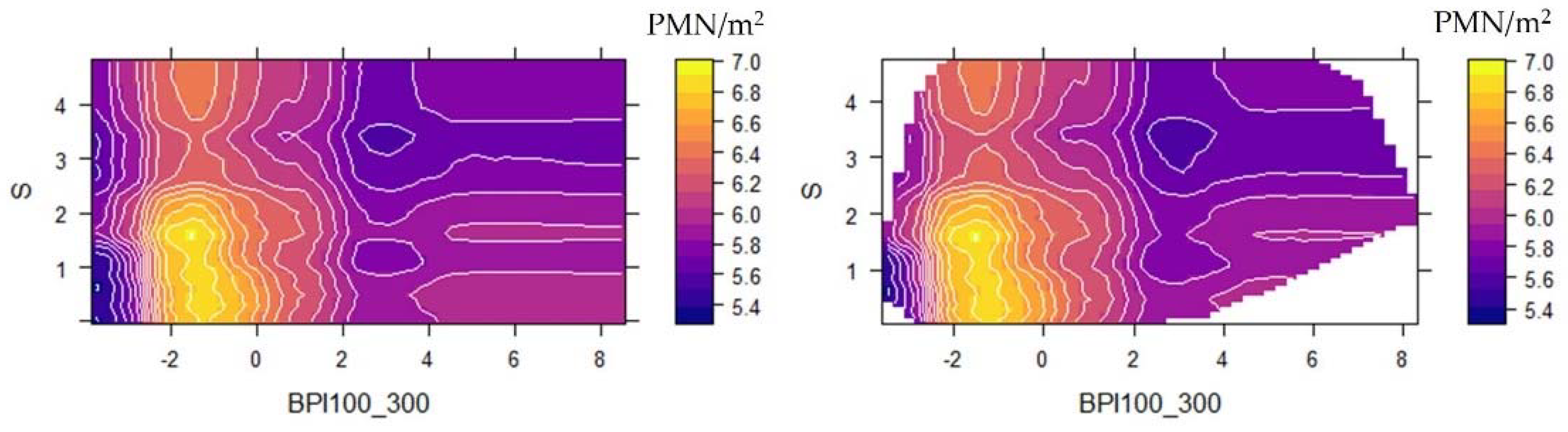
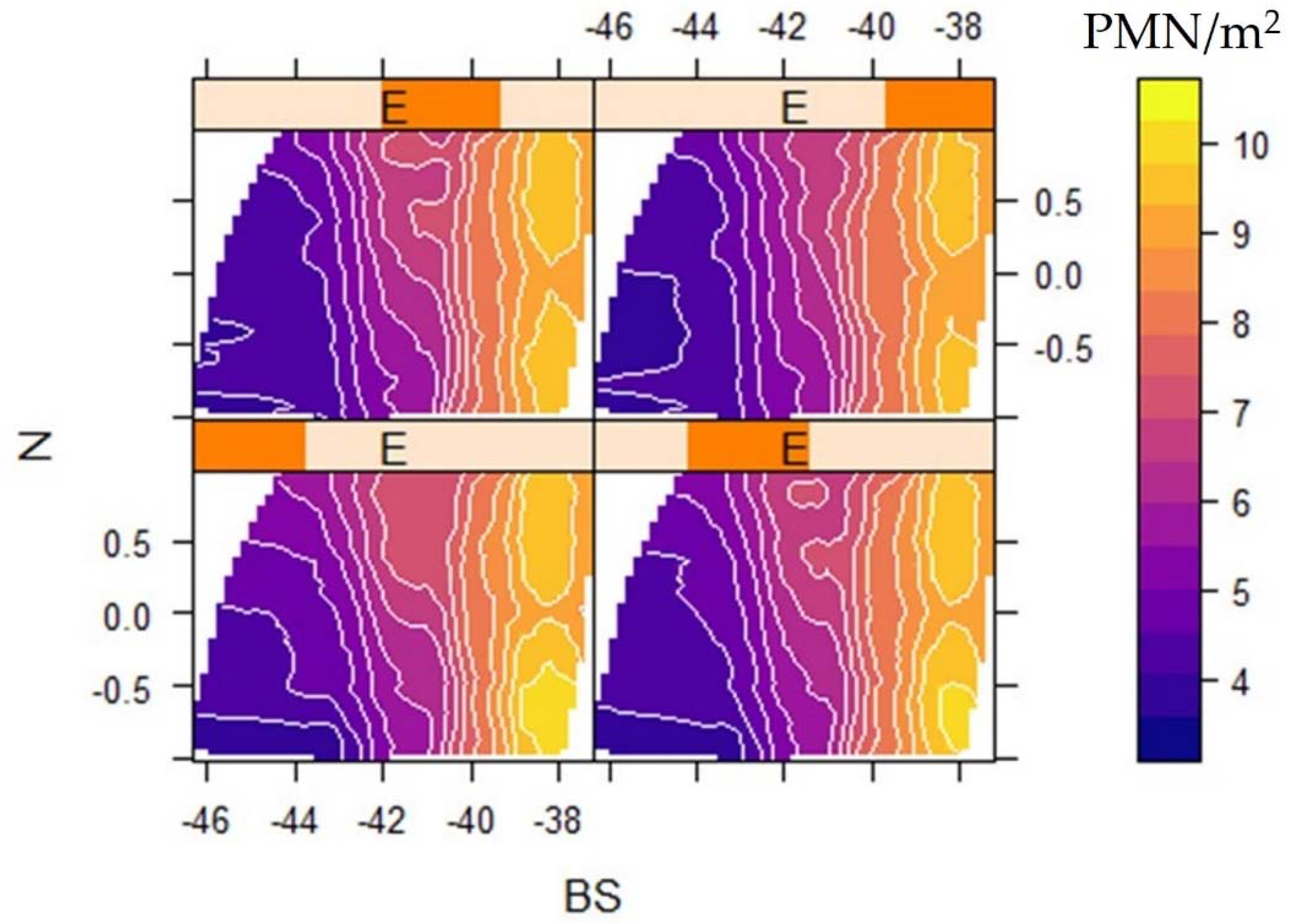
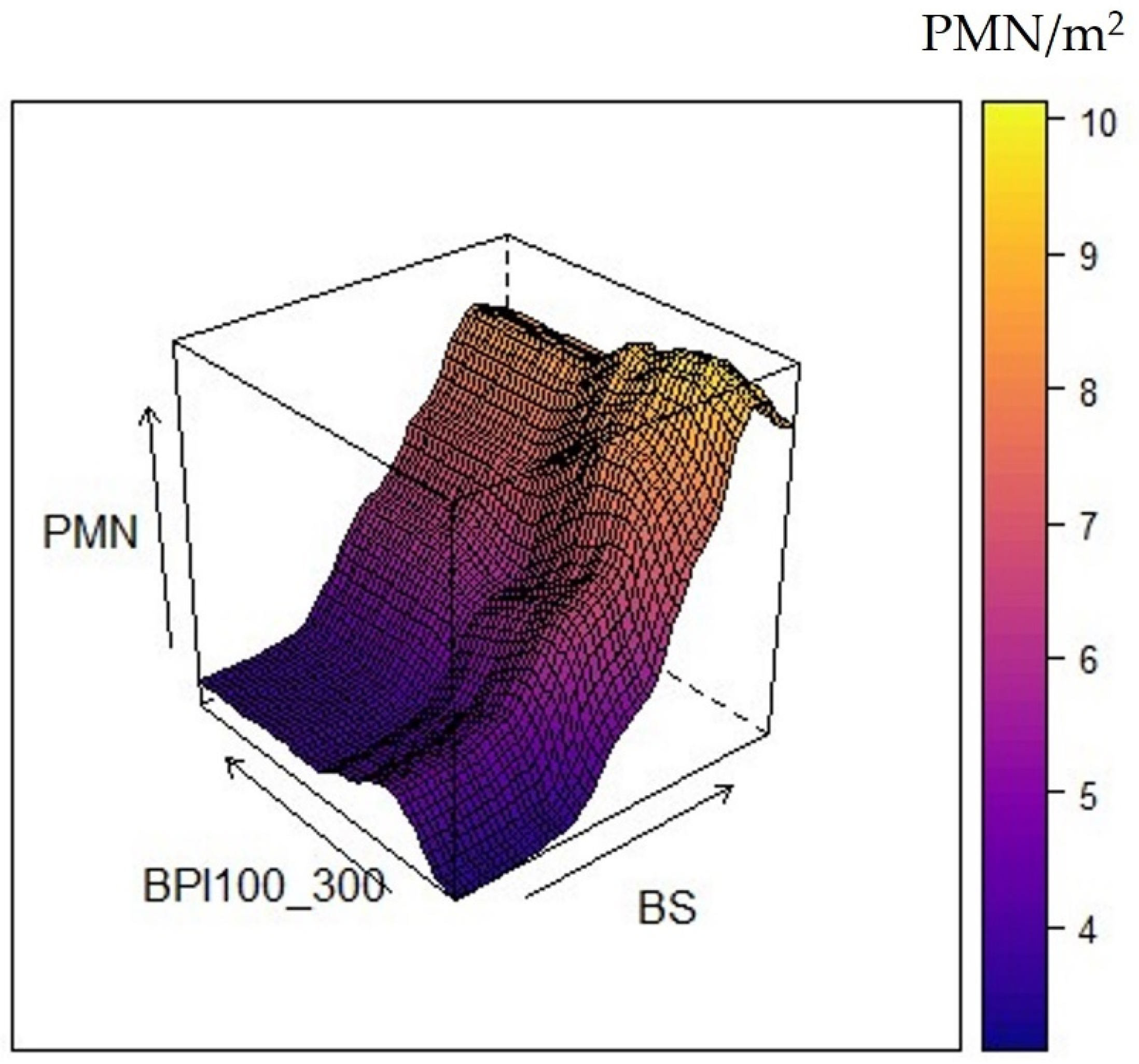
3.4. QRF Spatial Predictions and Uncertainty

The model prediction shows a heterogeneous PMN distribution, with a higher number of PMN aggregated in the northern and southern areas of the DEA that follow the overall seafloor topography and the bottom current regime (Figure 8). The lower and upper quantile predictions differ, with the 0.05th quantile being less affected by sampling artifacts, which are prominent in the 0.95th quantile. Moreover, the 0.05th and 0.50th quantile predict the spatial extent of PMN-free patches better (Figure 9). Inside the DEA, the central and southern parts have the lowest quantile difference, due to the increased sampling effort. The DEA-NE area also has parts with alternating high and low numbers of PMN (Figure 8). In Figure 10, the RF model results were plotted together with the visual observations from the ocean floor observation system, showing an overall spatial agreement. However, the predictions inside the DEA-NE area have high uncertainty, as the model has seen no training data from this area and the seafloor is morphologically more complex than the DEA (Figure 8).

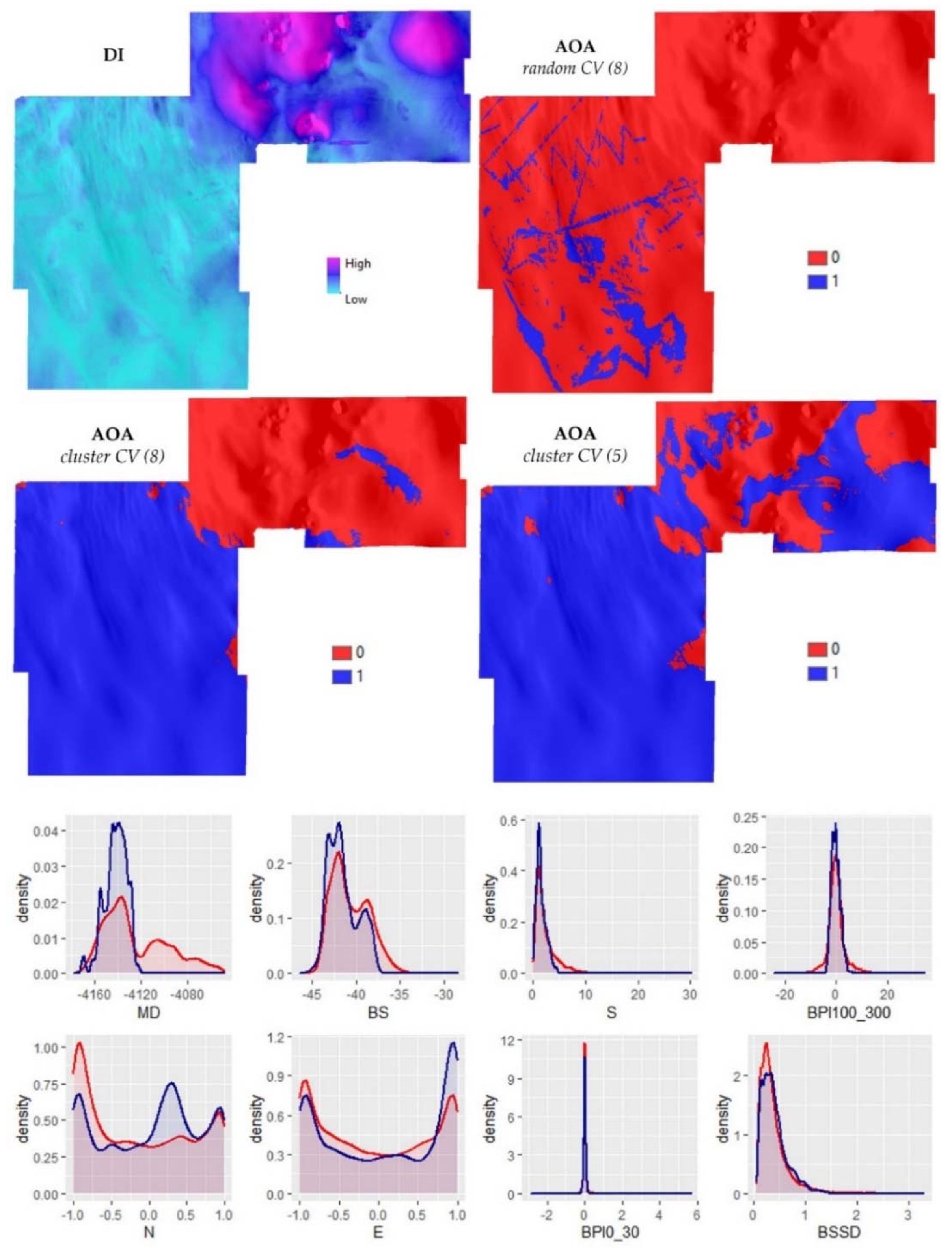
3.5. Dissimilarity Analysis and Area of Applicability

The dissimilarity analysis showed that the DEA-NE is dissimilar to the training samples, especially in the areas with rugged seafloor, increased slopes, and shallower bathymetric depth range. These circumstances reduce the area of applicability of the model, showing that additional samples must be added for better predictions. Data derived from the random-CV model have the smallest AOA. The overoptimistic error assessment that occurs limits the model AOA to a small region around the training locations, where the CV error is still small and comparable. Conversely, spatial- and cluster-CV have a larger prediction error. Hence, this error applies towards a wider area (Figure 11). The AOA also increased when excluding the MD, BSSD, and BPI0_30 features. The latter two were excluded due to their negligible contribution in the final model. Although, they are well sampled (Figure 11). MD was excluded, as the training samples do not cover the entire depth range of the study area (Figure 11). We have prior knowledge from video observations (e.g., Figure 10 and previous studies [62,63,69]) that the DEA-NE is inside the bathymetric depth range that favors the aggregation of PMN. The exclusion of the mean depth could provide a simpler and better transferable model (on local scales), putting a greater importance on relative bathymetric variations, such as local elevations and depressions expressed by the BPI. The exclusion of the three variables MD, BSSD, and BPI0_30 resulted in a decreased dissimilarity and a larger AOA (Figure 11), but the predictive performance for the test data was reduced (R² = 0.73). In general, several parts of the DEA-NE remain unsuitable for predictions using the developed model, due to the complex geomorphology and lack of samples that cover this complex terrain.

4. Discussion

This article presents a PMN prediction case study based on AUV hydroacoustic and image data from the Peru Basin in the Pacific. The study highlights the presence of spatial autocorrelation within the polymetallic nodule (PMN) distribution, with the PMN being spatially aggregated due to local geomorphological settings and the prevailing bottom current regime. The northwest oriented bottom current is channeled through abyssal furrows and erodes fine sediments. This leaves abundant fragmental materials (fish teeth, basalt debris, tiny pieces of broken shell, or nodules) as nuclei for the formation of PMN [134]. The higher number of PMN in the northern part of the DEA and DEA-NE is supported by the vicinity to seamounts (Figure 1), which provides additional nucleus material, initiating the nodule formation presence [135]. It is still unclear to what degree such influence has in comparison or synergistically to the geochemical properties of the sediment, which play an essential role in the PMN spatial distribution, their abundance, and size [134,136]. Using spatial geochemical information as input data in the modeling process would have been advantageous, as omitting such drivers limits the predictive performance. Unfortunately, the existing sampling methods (gravity cores, push cores, multi-cores, and box-corers) have limited spatial coverage, are typically clustered in small sub-regions due to the need for multiple replicates in biological studies, and generally do not occur in great numbers due to the time-consuming sampling (4–5 h per sample) and subsequent geochemical analyses.

Although our knowledge of the real reasons and their interrelationship with PMN formation is incomplete, analyzing the spatial autocorrelation has a strong potential to explore complex geomorphological relations, as it is an inherent part of the natural PMN distribution and variability across different spatial scales. In this respect, calculating the local Moran’s I can contribute in three ways:

(a) Local Moran’s I reveals significant PMN spatial clusters. Further investigation of such areas revealed the spatial dependency of PMN by the seafloor morphology (exogenous autocorrelation), as the MBES derivatives values differ significantly between the H-H and L-L groups.

(b) Local Moran’s I can effectively identify predictors for spatial modeling. In contrast, the non-spatial Boruta algorithm showed increased relevance in predictors such as the BSSD and BPI0_30 that had a minor to zero contribution in the final RF model.

(c) Local Moran’s I reduces the number of training samples needed. Only the data that contribute the most are kept, and the model becomes computationally lighter while its performance increases. Studies have highlighted the need for better data (i.e., representative with low sampling uncertainty and noise, having enough variation to capture critical patterns in the data, and well distributed across the entire feature space) in data-driven approaches such as geostatistical and ML predictive modeling [18,137,138]. In this respect, the local Moran’s I analysis could be an efficient tool.

Spatial autocorrelation (SAC) can help to address the issues mentioned above, at the same time not considering spatial autocorrelation may result in over-optimistic CV predictions. Similar to recent studies [17,19,20,21,23,24,139,140], we showed that the conventional and commonly applied random 10-fold CV could not assess the model performance when spatial autocorrelation is present. In such cases, spatial- and cluster-blocking perform better. Spatial-blocking is the least biased and results in lower variance than cluster-blocking; the higher variance of cluster-blocking has also been mentioned by others [17].

The spatial- and cluster-CV also yielded different mtry hyperparameter values. Five predictors were adequate to predict the hold-out samples inside the random (and identical) folders. However, for the spatial- and cluster-CV, all available predictors (eight) were needed. The final models have the same performance in the unseen (but similar) test data. By applying different CV methods, we changed our assessment method, not the model itself. This fact shows that a spatially similar test dataset can show how well the model can reproduce the data, but it cannot inform about how the model performs when it is transferred to another area. In this case, the spatial-CV is recommended.

The random-CV could still be preferable in case of a) small datasets with geographical separation within the training points that exceed the area of spatial autocorrelation (influence zone) or b) when the predictions are restricted to nearby locations of the training samples [20,33,141]. Random-CV is the most straightforward implementation. Contrasting spatial-blocking demands a prior correlogram calculation to identify the block size, and cluster-blocking demands the use of clustering indexes (e.g., Calinski–Harabasz) to find the optimum number of clusters along with data preprocessing (e.g., scaling of input MBES derivatives). These procedures usually demand the use of more than one software, increasing the time and complexity of the processing.

However, the biggest challenge lies in realizing the need for training data that are simultaneously well spread across the geographical and feature space of the covariates used for the analysis. Despite the significant advances in terrestrial spatial sampling [142,143,144,145,146], deep-sea studies have only lately started developing methods to optimize AUV photo sampling in a way that maximizes the environmental information [147,148,149,150]. In this respect, the QRF and AOA could guide sampling efforts in previously sampled areas or even during sampling surveys (adaptive sampling or/and active learning).

The poor representation of the feature space, especially the range of the most important predictor variables, causes a reduced performance and transferability of regression random forests modelling [151,152]. In our case, the dissimilarity analysis (DI and density curves) showed differences between the training samples and the targeted feature space. This becomes visible in the quantile uncertainty (QU), which is maximized in the DEA-NE. The QU is a helpful tool to explore the model variation inside the convex hull of the training points (Figure A8 and Figure A9). QU is correlated with DI (r = 0.65, p < 2.2 × 10⁻¹⁶). However, there are subareas inside the DEA-NE with high dissimilarity but no high analogue uncertainty. This is a misleading extrapolation effect that has been described by the AOA authors [35]. In other words, QRF can provide locations that have increased model variation, but it cannot identify if this is caused due to the inherent uncertainty of the hydroacoustic and image data or due to extrapolation.

Any model extrapolation beyond the training domain should be accompanied by a thorough transferability assessment, ideally with an external evaluation using data from the new area [22,33,153]. This was not possible here, due to a lack of data. Instead, we used the recently proposed AOA method. Within the DEA-NE area, the expected prediction error is higher than in the trained area of the DEA, reducing the model applicability. The exclusion of predictors that are prone to overfitting, such as elevation/depth, increases the generalization performance, which has also been mentioned by [22]. The advantage of RF to build complex non-linear response curves with the training data, outperforming other regression methods [154], could result in a disadvantage when these associations occur only locally [155]. A successful transfer thus relies on the assumption that the relationship between response variable and predictor exists in both areas. The generalization performance is maximized when the data information and feature selection are combined with the domain knowledge, even if the domain knowledge is basic or imperfect [156,157]. Other studies also showed that machine learning models with only a few predictor variables are more transferable in marine habitat mapping than complex ones [158].

Similarly, less complex models (e.g., partial least squares regression) could generalize better when spatial-CV schemes are applied, highlighting the trade-off decision to be made between accuracy and generalization performance [21,25,27]. Similarly, ensemble ML models that average predictions of different single models could also yield better predictions across different areas, as presented by [23,141]. The comparison of different models was beyond the scope of this paper. Here, we focused on the widely used random forests algorithm and its quantile uncertainty (i.e., QRF). We should underline that transferability is not the primary goal when applying machine learning-based spatial modelling. ML is designed to derive accurate predictions based on an existing measurement that captures the underlying relationship, for which our knowledge or conceptual understanding is still developing. Towards this direction, the RF importance score is a valuable measure to test known hypotheses, but also to generate new ones [155,159,160].

Future research in other parts of the Peru Basin and other known fields with polymetallic nodules (e.g., the Clarion-Clipperton Zone) could further enlighten the drivers of spatial autocorrelation. In addition, the spatial analysis in various scales would also provide insights for the underlying mechanisms that influence the spatial distribution of polymetallic nodules.

5. Conclusions

Our case study shows that spatial predictions of polymetallic nodules with ML methods need to be spatial-cross-validated when the spatial autocorrelation is present, and that the seafloor morphology varies. Similarly, model transfer to areas with scarce or no data should be evaluated by regarding the new area similarity with the training domain. Ideally, each ML predictive spatial map should be accompanied with its cross-validation strategy, uncertainty prediction, and area of application analyses, for supporting the model interpretation and decision making. In other words, the focus should not only lie in generating the final prediction map, but also on how this map has been derived from the fitted model and data.

References

1. Hein, J.R.; Koschinsky, A.; Kuhn, T. Deep-ocean polymetallic nodules as a resource for critical materials. Nat. Rev. Earth Environ. 2020, 1, 158–169. [Google Scholar] [CrossRef]
2. Hein, J.R.; Mizell, K.; Koschinsky, A.; Conrad, T.A. Deep-ocean mineral deposits as a source of critical metals for high- and green-technology applications: Comparison with land-based resources. Ore Geol. Rev. 2013, 51, 1–14. [Google Scholar] [CrossRef]
3. EC Communication COM, 474, F. Critical Raw Materials Resilience: Charting a Path towards Greater Security and Sustainability. 2020. Available online: https://eur-lex.europa.eu/legal-content/EN/TXT/HTML/?uri=CELEX:52020DC0474&from=EN (accessed on 30 August 2021).
4. Schoening, T.; Purser, A.; Langenkämper, D.; Suck, I.; Taylor, J.; Cuvelier, D.; Lins, L.; Simon-Lledó, E.; Marcon, Y.; Jones, D.O.B.; et al. Megafauna community assessment of polymetallic-nodule fields with cameras: Platform and methodology comparison. Biogeosciences 2020, 17, 3115–3133. [Google Scholar] [CrossRef]
5. Schoening, T.; Köser, K.; Greinert, J. An acquisition, curation and management workflow for sustainable, terabyte-scale marine image analysis. Sci. Data 2018, 5, 180181. [Google Scholar] [CrossRef] [PubMed]
6. Simon-Lledó, E.; Bett, B.J.; Huvenne, V.A.I.; Köser, K.; Schoening, T.; Greinert, J.; Jones, D.O.B. Biological effects 26 years after simulated deep-sea mining. Sci. Rep. 2019, 9, 8040. [Google Scholar] [CrossRef] [PubMed]
7. Gazis, I.Z.; Schoening, T.; Alevizos, E.; Greinert, J. Quantitative mapping and predictive modeling of Mn nodules’ distribution from hydroacoustic and optical AUV data linked by random forests machine learning. Biogeosciences 2018, 15, 7347–7377. [Google Scholar] [CrossRef] [Green Version]
8. Peukert, A.; Schoening, T.; Alevizos, E.; Köser, K.; Kwasnitschka, T.; Greinert, J. Understanding Mn-nodule distribution and evaluation of related deep-sea mining impacts using AUV-based hydroacoustic and optical data. Biogeosciences 2018, 15, 2525–2549. [Google Scholar] [CrossRef] [Green Version]
9. Schoening, T.; Jones, D.O.B.; Greinert, J. Compact-Morphology-based poly-metallic Nodule Delineation. Sci. Rep. 2017, 7, 13338. [Google Scholar] [CrossRef]
10. Hari, V.N.; Kalyan, B.; Chitre, M.; Ganesan, V. Spatial Modeling of Deep-Sea Ferromanganese Nodules with Limited Data Using Neural Networks. IEEE J. Ocean. Eng. 2018, 43, 997–1014. [Google Scholar] [CrossRef]
11. Kaikkonen, L.; Virtanen, E.A.; Kostamo, K.; Lappalainen, J.; Kotilainen, A.T. Extensive Coverage of Marine Mineral Concretions Revealed in Shallow Shelf Sea Areas. Front. Mar. Sci. 2019, 6, 541. [Google Scholar] [CrossRef]
12. Wong, L.J.; Kalyan, B.; Chitre, M.; Vishnu, H. Acoustic Assessment of Polymetallic Nodule Abundance Using Sidescan Sonar and Altimeter. IEEE J. Ocean. Eng. 2021, 46, 132–142. [Google Scholar] [CrossRef]
13. Dutkiewicz, A.; Judge, A.; Müller, R.D. Environmental predictors of deep-sea polymetallic nodule occurrence in the global ocean. Geology 2020, 48, 293–297. [Google Scholar] [CrossRef]
14. Wasilewska-Błaszczyk, M.; Mucha, J. Application of General Linear Models (GLM) to assess nodule abundance based on a photographic survey (case study from IOM Area, Pacific Ocean). Minerals 2021, 11, 427. [Google Scholar] [CrossRef]
15. Kuhn, T.; Rühlemann, C. Exploration of polymetallic nodules and resource assessment: A case study from the German contract area in the clarion-clipperton zone of the tropical northeast pacific. Minerals 2021, 11, 618. [Google Scholar] [CrossRef]
16. Anselin, L. Local Indicators of Spatial Association-LISA. Geogr. Anal. 1995, 27, 93–115. [Google Scholar] [CrossRef]
17. Roberts, D.R.; Bahn, V.; Ciuti, S.; Boyce, M.S.; Elith, J.; Guillera-Arroita, G.; Hauenstein, S.; Lahoz-Monfort, J.J.; Schröder, B.; Thuiller, W.; et al. Cross-validation strategies for data with temporal, spatial, hierarchical, or phylogenetic structure. Ecography 2017, 40, 913–929. [Google Scholar] [CrossRef]
18. Hengl, T.; Nussbaum, M.; Wright, M.N.; Heuvelink, G.B.M.; Gräler, B. Random forest as a generic framework for predictive modeling of spatial and spatio-temporal variables. PeerJ 2018, 6, e5518. [Google Scholar] [CrossRef] [Green Version]
19. Meyer, H.; Reudenbach, C.; Hengl, T.; Katurji, M.; Nauss, T. Improving performance of spatio-temporal machine learning models using forward feature selection and target-oriented validation. Environ. Model. Softw. 2018, 101, 1–9. [Google Scholar] [CrossRef]
20. Misiuk, B.; Diesing, M.; Aitken, A.; Brown, C.J.; Edinger, E.N.; Bell, T. A Spatially Explicit Comparison of Quantitative and Categorical Modelling Approaches for Mapping Seabed Sediments Using Random Forest. Geosciences 2019, 9, 254. [Google Scholar] [CrossRef] [Green Version]
21. Ploton, P.; Mortier, F.; Réjou-Méchain, M.; Barbier, N.; Picard, N.; Rossi, V.; Dormann, C.; Cornu, G.; Viennois, G.; Bayol, N.; et al. Spatial validation reveals poor predictive performance of large-scale ecological mapping models. Nat. Commun. 2020, 11, 4540. [Google Scholar] [CrossRef]
22. Wenger, S.J.; Olden, J.D. Assessing transferability of ecological models: An underappreciated aspect of statistical validation. Methods Ecol. Evol. 2012, 3, 260–267. [Google Scholar] [CrossRef]
23. Hao, T.; Elith, J.; Lahoz-Monfort, J.J.; Guillera-Arroita, G. Testing whether ensemble modelling is advantageous for maximising predictive performance of species distribution models. Ecography 2020, 43, 549–558. [Google Scholar] [CrossRef] [Green Version]
24. Dolan, M.F.J.; Ross, R.E.; Albretsen, J.; Skarðhamar, J.; Gonzalez-Mirelis, G.; Bellec, V.K.; Buhl-Mortensen, P.; Bjarnadóttir, L.R. Using Spatial Validity and Uncertainty Metrics to Determine the Relative Suitability of Alternative Suites of Oceanographic Data for Seabed Biotope Prediction. A Case Study from the Barents Sea, Norway. Geosciences 2021, 11, 48. [Google Scholar] [CrossRef]
25. Schratz, P.; Muenchow, J.; Iturritxa, E.; Richter, J.; Brenning, A. Hyperparameter tuning and performance assessment of statistical and machine-learning algorithms using spatial data. Ecol. Modell. 2019, 406, 109–120. [Google Scholar] [CrossRef] [Green Version]
26. Pohjankukka, J.; Pahikkala, T.; Nevalainen, P.; Heikkonen, J. Estimating the prediction performance of spatial models via spatial k-fold cross validation. Int. J. Geogr. Inf. Sci. 2017, 31, 2001–2019. [Google Scholar] [CrossRef]
27. Parmentier, I.; Harrigan, R.J.; Buermann, W.; Mitchard, E.T.A.; Saatchi, S.; Malhi, Y.; Bongers, F.; Hawthorne, W.D.; Leal, M.E.; Lewis, S.L.; et al. Predicting alpha diversity of African rain forests: Models based on climate and satellite-derived data do not perform better than a purely spatial model. J. Biogeogr. 2011, 38, 1164–1176. [Google Scholar] [CrossRef]
28. Trachsel, M.; Telford, R.J. Technical note: Estimating unbiased transfer-function performances in spatially structured environments. Clim. Past 2016, 12, 1215–1223. [Google Scholar] [CrossRef] [Green Version]
29. Le Rest, K.; Pinaud, D.; Monestiez, P.; Chadoeuf, J.; Bretagnolle, V. Spatial leave-one-out cross-validation for variable selection in the presence of spatial autocorrelation. Glob. Ecol. Biogeogr. 2014, 23, 811–820. [Google Scholar] [CrossRef] [Green Version]
30. Ruß, G.; Brenning, A. Spatial Variable Importance Assessment for Yield Prediction in Precision Agriculture. In Advances in Intelligent Data Analysis IX; Lecture Notes in Computer Science; Cohen, P.R., Adams, N.M., Berthold, M.R., Eds.; Springer: Berlin/Heidelberg, Germany, 2010; Volume 6065. [Google Scholar] [CrossRef]
31. Valavi, R.; Elith, J.; Lahoz-Monfort, J.J.; Guillera-Arroita, G. blockCV: An r package for generating spatially or environmentally separated folds for k-fold cross-validation of species distribution models. Methods Ecol. Evol. 2019, 10, 225–232. [Google Scholar] [CrossRef] [Green Version]
32. Meyer, H.; Reudenbach, C.; Wöllauer, S.; Nauss, T. Importance of spatial predictor variable selection in machine learning applications—Moving from data reproduction to spatial prediction. Ecol. Modell. 2019, 411, 108815. [Google Scholar] [CrossRef] [Green Version]
33. Randin, C.F.; Dirnböck, T.; Dullinger, S.; Zimmermann, N.E.; Zappa, M.; Guisan, A. Are niche-based species distribution models transferable in space? J. Biogeogr. 2006, 33, 1689–1703. [Google Scholar] [CrossRef]
34. Yates, K.L.; Bouchet, P.J.; Caley, M.J.; Mengersen, K.; Randin, C.F.; Parnell, S.; Fielding, A.H.; Bamford, A.J.; Ban, S.; Barbosa, A.M.; et al. Outstanding Challenges in the Transferability of Ecological Models. Trends Ecol. Evol. 2018, 33, 790–802. [Google Scholar] [CrossRef] [Green Version]
35. Meyer, H.; Pebesma, E. Predicting into unknown space? Estimating the area of applicability of spatial prediction models. Methods Ecol. Evol. 2021, 12, 2041–2210. [Google Scholar] [CrossRef]
36. Kuhn, M.; Johnson, K. Applied Predictive Modeling; Springer: New York, NY, USA, 2013; ISBN 978-1-4614-6848-6. [Google Scholar]
37. Elith, J.; Kearney, M.; Phillips, S. The art of modelling range-shifting species. Methods Ecol. Evol. 2010, 1, 330–342. [Google Scholar] [CrossRef]
38. Zurell, D.; Elith, J.; Schröder, B. Predicting to new environments: Tools for visualizing model behaviour and impacts on mapped distributions. Divers. Distrib. 2012, 18, 628–634. [Google Scholar] [CrossRef]
39. Owens, H.L.; Campbell, L.P.; Dornak, L.L.; Saupe, E.E.; Barve, N.; Soberón, J.; Ingenloff, K.; Lira-Noriega, A.; Hensz, C.M.; Myers, C.E.; et al. Constraints on interpretation of ecological niche models by limited environmental ranges on calibration areas. Ecol. Modell. 2013, 263, 10–18. [Google Scholar] [CrossRef]
40. Mesgaran, M.B.; Cousens, R.D.; Webber, B.L. Here be dragons: A tool for quantifying novelty due to covariate range and correlation change when projecting species distribution models. Divers. Distrib. 2014, 20, 1147–1159. [Google Scholar] [CrossRef]
41. Rödder, D.; Engler, J.O. Disentangling Interpolation and Extrapolation Uncertainties in Species Distribution Models: A Novel Visualization Technique for the Spatial Variation of Predictor Variable Colinearity. Biodivers. Inform. 2012, 8, 4326. [Google Scholar] [CrossRef] [Green Version]
42. Wilcoxon, F. Individual Comparisons by Ranking Methods. Biom. Bull. 1945, 1, 80. [Google Scholar] [CrossRef]
43. Mann, H.B.; Whitney, D.R. On a Test of Whether one of Two Random Variables is Stochastically Larger than the Other. Ann. Math. Stat. 1947, 18, 50–60. [Google Scholar] [CrossRef]
44. Kruskal, W.H. Historical Notes on the Wilcoxon Unpaired Two-Sample Test. J. Am. Stat. Assoc. 1957, 52, 356. [Google Scholar] [CrossRef]
45. Kursa, M.B.; Rudnicki, W.R. Feature Selection with the Boruta Package. J. Stat. Softw. 2010, 36, 11. [Google Scholar] [CrossRef] [Green Version]
46. Kursa, M.B. Robustness of Random Forest-based gene selection methods. BMC Bioinform. 2014, 15, 8. [Google Scholar] [CrossRef] [PubMed] [Green Version]
47. Degenhardt, F.; Seifert, S.; Szymczak, S. Evaluation of variable selection methods for random forests and omics data sets. Brief. Bioinform. 2019, 20, 492–503. [Google Scholar] [CrossRef] [PubMed] [Green Version]
48. Li, J.; Tran, M.; Siwabessy, J. Selecting Optimal Random Forest Predictive Models: A Case Study on Predicting the Spatial Distribution of Seabed Hardness. PLoS ONE 2016, 11, e0149089. [Google Scholar] [CrossRef]
49. Li, J.; Alvarez, B.; Siwabessy, J.; Tran, M.; Huang, Z.; Przeslawski, R.; Radke, L.; Howard, F.; Nichol, S. Application of random forest, generalised linear model and their hybrid methods with geostatistical techniques to count data: Predicting sponge species richness. Environ. Model. Softw. 2017, 97, 112–129. [Google Scholar] [CrossRef]
50. Li, J. A Critical Review of Spatial Predictive Modeling Process in Environmental Sciences with Reproducible Examples in R. Appl. Sci. 2019, 9, 2048. [Google Scholar] [CrossRef] [Green Version]
51. Diesing, M.; Thorsnes, T. Mapping of Cold-Water Coral Carbonate Mounds Based on Geomorphometric Features: An Object-Based Approach. Geosciences 2018, 8, 34. [Google Scholar] [CrossRef] [Green Version]
52. Diesing, M.; Mitchell, P.J.; O’Keeffe, E.; Gavazzi, G.O.A.M.; Bas, T. Le Limitations of Predicting Substrate Classes on a Sedimentary Complex but Morphologically Simple Seabed. Remote Sens. 2020, 12, 3398. [Google Scholar] [CrossRef]
53. Diesing, M. Deep-sea sediments of the global ocean. Earth Syst. Sci. Data 2020, 12, 3367–3381. [Google Scholar] [CrossRef]
54. Breiman, L. Random forests. Mach. Learn. 2001, 45, 5–32. [Google Scholar] [CrossRef] [Green Version]
55. Meinshausen, N. Quantile regression forests. J. Mach. Learn. Res. 2006, 7, 983–999. [Google Scholar]
56. Kirkwood, C.; Cave, M.; Beamish, D.; Grebby, S.; Ferreira, A. A machine learning approach to geochemical mapping. J. Geochem. Explor. 2016, 167, 49–61. [Google Scholar] [CrossRef] [Green Version]
57. Vaysse, K.; Lagacherie, P. Using quantile regression forest to estimate uncertainty of digital soil mapping products. Geoderma 2017, 291, 55–64. [Google Scholar] [CrossRef]
58. Fouedjio, F.; Klump, J. Exploring prediction uncertainty of spatial data in geostatistical and machine learning approaches. Environ. Earth Sci. 2019, 78, 38. [Google Scholar] [CrossRef]
59. Szatmári, G.; Pásztor, L. Comparison of various uncertainty modelling approaches based on geostatistics and machine learning algorithms. Geoderma 2019, 337, 1329–1340. [Google Scholar] [CrossRef]
60. Diesing, M.; Kröger, S.; Parker, R.; Jenkins, C.; Mason, C.; Weston, K. Predicting the standing stock of organic carbon in surface sediments of the North–West European continental shelf. Biogeochemistry 2017, 135, 183–200. [Google Scholar] [CrossRef] [Green Version]
61. Baker, E.; Beaudoin, Y. Deep Sea Minerals: A Physical, Biological, Environmental, and Technical Review; Secretariat of the Pacific Community: Suva, Fiji, 2013; ISBN 978-827-701-12-02. [Google Scholar]
62. Marchig, V.; Reyss, J.L. Diagenetic mobilization of manganese in Peru Basin sediments. Geochim. Cosmochim. Acta 1984, 48, 1349–1352. [Google Scholar] [CrossRef]
63. Von Stackelberg, U. Growth history of manganese nodules and crusts of the Peru Basin. Geol. Soc. Lond. Spec. Publ. 1997, 119, 153–176. [Google Scholar] [CrossRef]
64. Weber, M.; von Stackelberg, U.; Marchig, V.; Wiedicke, M.; Grupe, B. Variability of surface sediments in the Peru basin: Dependence on water depth, productivity, bottom water flow, and seafloor topography. Mar. Geol. 2000, 163, 169–184. [Google Scholar] [CrossRef]
65. Toro, N.; Jeldres, R.I.; Órdenes, J.A.; Robles, P.; Navarra, A. Manganese Nodules in Chile, an Alternative for the Production of Co and Mn in the Future—A Review. Minerals 2020, 10, 674. [Google Scholar] [CrossRef]
66. Thiel, H.; Schriever, G.; Ahnert, A.; Bluhm, H.; Borowski, C.; Vopel, K. The large-scale environmental impact experiment DISCOL—reflection and foresight. Deep Sea Res. Part II Top. Stud. Oceanogr. 2001, 48, 3869–3882. [Google Scholar] [CrossRef]
67. Gausepohl, F.; Hennke, A.; Schoening, T.; Köser, K.; Greinert, J. Scars in the abyss: Reconstructing sequence, location and temporal change of the 78 plough tracks of the 1989 DISCOL deep-sea disturbance experiment in the Peru Basin. Biogeosciences 2020, 17, 1463–1493. [Google Scholar] [CrossRef] [Green Version]
68. Wiedicke, M.H.; Weber, M.E. Small-scale variability of seafloor features in the northern Peru Basin: Results from acoustic survey methods. Mar. Geophys. Res. 1996, 18, 507–526. [Google Scholar] [CrossRef]
69. Paul, S.A.L.; Haeckel, M.; Bau, M.; Bajracharya, R.; Koschinsky, A. Small-scale heterogeneity of trace metals including rare earth elements and yttrium in deep-sea sediments and porewaters of the Peru Basin, southeastern equatorial Pacific. Biogeosciences 2019, 16, 4829–4849. [Google Scholar] [CrossRef] [Green Version]
70. Grupe, B.; Becker, H.J.; Oebius, H.U. Geotechnical and sedimentological investigations of deep-sea sediments from a manganese nodule field of the Peru Basin. Deep Sea Res. Part II Top. Stud. Oceanogr. 2001, 48, 3593–3608. [Google Scholar] [CrossRef]
71. Klein, H. Near-bottom currents in the deep Peru Basin, DISCOL experimental area. Dtsch. Hydrogr. Z. 1993, 45, 31–42. [Google Scholar] [CrossRef]
72. Klein, H. Near-bottom currents and bottom boundary layer variability over manganese nodule fields in the peru basin, se-pacific. Dtsch. Hydrogr. Z. 1996, 48, 147–160. [Google Scholar] [CrossRef]
73. Flood, R.D. Classification of sedimentary furrows and a model for furrow initiation and evolution. Geol. Soc. Am. Bull. 1983, 94, 630. [Google Scholar] [CrossRef]
74. Lonsdale, P.; Spiess, F.N. Abyssal Bedforms Explored with a Deeply Towed Instrument Package. Dev. Sedimentol. 1977, 23, 57–75. [Google Scholar]
75. Flood, R.D.; Hollister, C.D. Submersible studies of deep-sea furrows and transverse ripples in cohesive sediments. Mar. Geol. 1980, 36, M1–M9. [Google Scholar] [CrossRef]
76. Haeckel, M.; König, I.; Riech, V.; Weber, M.E.; Suess, E. Pore water profiles and numerical modelling of biogeochemical processes in Peru Basin deep-sea sediments. Deep Sea Res. Part II Top. Stud. Oceanogr. 2001, 48, 3713–3736. [Google Scholar] [CrossRef]
77. Greinert, J. RV Sonne Fahrtbericht/Cruise Report SO242-1 [SO242/1], JPI Oceans Ecological Aspects of Deep-Sea Mining, DISCOL Revisited, Guayaquil-Guayaquil, 28 July–25 August 2015; GEOMAR Report, N. Ser. 026; GEOMAR Helmholtz-Zentrum für Ozeanforschung: Kiel, Germany, 2015; Volume 7. [Google Scholar]
78. Benites, M.; Millo, C.; Hein, J.; Nath, B.; Murton, B.; Galante, D.; Jovane, L. Integrated Geochemical and Morphological Data Provide Insights into the Genesis of Ferromanganese Nodules. Minerals 2018, 8, 488. [Google Scholar] [CrossRef] [Green Version]
79. Burdige, D.J. The biogeochemistry of manganese and iron reduction in marine sediments. Earth-Sci. Rev. 1993, 35, 249–284. [Google Scholar] [CrossRef]
80. Linke, P.; Lackschewitz, K. Autonomous Underwater Vehicle “ABYSS”. J. Large-Scale Res. Facil. 2016, 2, A79. [Google Scholar] [CrossRef] [Green Version]
81. Klischies, M.; Rothenbeck, M.; Steinfuhrer, A.; Yeo, I.A.; dos Santos Ferreira, C.; Mohrmann, J.; Faber, C.; Schirnick, C. AUV Abyss workflow: Autonomous deep sea exploration for ocean research. In Proceedings of the 2018 IEEE/OES Autonomous Underwater Vehicle Workshop (AUV), Porto, Portugal, 6–9 November 2018; pp. 1–6. [Google Scholar]
82. Caress, D.W.; Chayes, D.N. MB-System: Mapping the Seafloor. 2017. Available online: http://www.mbari.org/products/research-software/mb-system/ (accessed on 18 October 2021).
83. Alevizos, E.; Schoening, T.; Koeser, K.; Snellen, M.; Greinert, J. Quantification of the fine-scale distribution of Mn-nodules: Insights from AUV multi-beam and optical imagery data fusion. Biogeosciences 2018, 1–29. [Google Scholar] [CrossRef] [Green Version]
84. Lecours, V.; Dolan, M.F.J.; Micallef, A.; Lucieer, V.L. A review of marine geomorphometry, the quantitative study of the seafloor. Hydrol. Earth Syst. Sci. 2016, 20, 3207–3244. [Google Scholar] [CrossRef] [Green Version]
85. Iwahashi, J.; Pike, R.J. Automated classifications of topography from DEMs by an unsupervised nested-means algorithm and a three-part geometric signature. Geomorphology 2007, 86, 409–440. [Google Scholar] [CrossRef]
86. Dolan, M.F.J.; Lucieer, V.L. Variation and Uncertainty in Bathymetric Slope Calculations Using Geographic Information Systems. Mar. Geod. 2014, 37, 187–219. [Google Scholar] [CrossRef]
87. Naimi, B.; Skidmore, A.K.; Groen, T.A.; Hamm, N.A.S. Spatial autocorrelation in predictors reduces the impact of positional uncertainty in occurrence data on species distribution modelling. J. Biogeogr. 2011, 38, 1497–1509. [Google Scholar] [CrossRef]
88. Stephens, D.; Diesing, M. A Comparison of Supervised Classification Methods for the Prediction of Substrate Type Using Multibeam Acoustic and Legacy Grain-Size Data. PLoS ONE 2014, 9, e93950. [Google Scholar] [CrossRef]
89. Lucieer, V.; Huang, Z.; Siwabessy, J. Analyzing Uncertainty in Multibeam Bathymetric Data and the Impact on Derived Seafloor Attributes. Mar. Geod. 2016, 39, 32–52. [Google Scholar] [CrossRef]
90. Lecours, V.; Devillers, R.; Edinger, E.N.; Brown, C.J.; Lucieer, V.L. Influence of artefacts in marine digital terrain models on habitat maps and species distribution models: A multiscale assessment. Remote Sens. Ecol. Conserv. 2017, 3, 232–246. [Google Scholar] [CrossRef]
91. Hughes Clarke, J. The Impact of Acoustic Imaging Geometry on the Fidelity of Seabed Bathymetric Models. Geosciences 2018, 8, 109. [Google Scholar] [CrossRef] [Green Version]
92. Florinsky, I.V. An illustrated introduction to general geomorphometry. Prog. Phys. Geogr. 2017, 41, 723–752. [Google Scholar] [CrossRef]
93. Misiuk, B.; Lecours, V.; Bell, T. A multiscale approach to mapping seabed sediments. PLoS ONE 2018, 13, e0193647. [Google Scholar] [CrossRef] [Green Version]
94. Cremers, J.; Klugkist, I. One Direction? A Tutorial for Circular Data Analysis Using R With Examples in Cognitive Psychology. Front. Psychol. 2018, 9. [Google Scholar] [CrossRef] [PubMed]
95. Zevenbergen, L.W.; Thorne, C.R. Quantitative analysis of land surface topography. Earth Surf. Process. Landf. 1987, 12, 47–56. [Google Scholar] [CrossRef]
96. Olaya, V. Chapter 6 Basic Land-Surface Parameters. Dev. Soil Sci. 2009, 33, 141–169. [Google Scholar]
97. Sappington, J.M.; Longshore, K.M.; Thompson, D.B. Quantifying Landscape Ruggedness for Animal Habitat Analysis: A Case Study Using Bighorn Sheep in the Mojave Desert. J. Wildl. Manage. 2007, 71, 1419–1426. [Google Scholar] [CrossRef]
98. Weiss, A. Topographic position and landforms analysis. Poster Present. ESRI User Conf. 2001, 64, 227–245. [Google Scholar]
99. Wilson, M.F.J.; O’Connell, B.; Brown, C.; Guinan, J.C.; Grehan, A.J. Multiscale Terrain Analysis of Multibeam Bathymetry Data for Habitat Mapping on the Continental Slope. Mar. Geod. 2007, 30, 3–35. [Google Scholar] [CrossRef] [Green Version]
100. Haralick, R.M.; Shanmugam, K.; Dinstein, I. Textural Features for Image Classification. IEEE Trans. Syst. Man. Cybern. 1973, SMC-3, 610–621. [Google Scholar] [CrossRef] [Green Version]
101. Conrad, O.; Bechtel, B.; Bock, M.; Dietrich, H.; Fischer, E.; Gerlitz, L.; Wehberg, J.; Wichmann, V.; Böhner, J. System for Automated Geoscientific Analyses (SAGA) v. 2.1.4. Geosci. Model Dev. 2015, 8, 1991–2007. [Google Scholar] [CrossRef] [Green Version]
102. Walbridge, S.; Slocum, N.; Pobuda, M.; Wright, D. Unified Geomorphological Analysis Workflows with Benthic Terrain Modeler. Geosciences 2018, 8, 94. [Google Scholar] [CrossRef] [Green Version]
103. Hijmans, R.J. Raster: Geographic Data Analysis and Modeling. R Package Version 3.4-13. 2021. Available online: https://CRAN.R-project.org/package=raster (accessed on 19 October 2021).
104. Zvoleff, A. glcm: Calculate Textures from Grey-Level Co-Occurrence Matrices (GLCMs). R Package Version 1.6.5. 2020. Available online: https://CRAN.R-project.org/package=glcm (accessed on 19 October 2021).
105. Kwasnitschka, T.; Köser, K.; Sticklus, J.; Rothenbeck, M.; Weiß, T.; Wenzlaff, E.; Schoening, T.; Triebe, L.; Steinführer, A.; Devey, C.; et al. DeepSurveyCam—A Deep Ocean Optical Mapping System. Sensors 2016, 16, 164. [Google Scholar] [CrossRef] [Green Version]
106. Ellefmo, S.L.; Kuhn, T. Application of Soft Data in Nodule Resource Estimation. Nat. Resour. Res. 2021, 30, 1069–1091. [Google Scholar] [CrossRef]
107. Wasilewska-Błaszczyk, M.; Mucha, J. Possibilities and Limitations of the Use of Seafloor Photographs for Estimating Polymetallic Nodule Resources—Case Study from IOM Area, Pacific Ocean. Minerals 2020, 10, 1123. [Google Scholar] [CrossRef]
108. Yu, G.; Parianos, J. Empirical Application of Generalized Rayleigh Distribution for Mineral Resource Estimation of Seabed Polymetallic Nodules. Minerals 2021, 11, 449. [Google Scholar] [CrossRef]
109. Tsune, A. Quantitative Expression of the Burial Phenomenon of Deep Seafloor Manganese Nodules. Minerals 2021, 11, 227. [Google Scholar] [CrossRef]
110. Simon-Lledó, E.; Bett, B.J.; Huvenne, V.A.I.; Schoening, T.; Benoist, N.M.A.; Jones, D.O.B. Ecology of a polymetallic nodule occurrence gradient: Implications for deep-sea mining. Limnol. Oceanogr. 2019, 64, 1883–1894. [Google Scholar] [CrossRef] [Green Version]
111. Caldas de Castro, M.; Singer, B.H. Controlling the False Discovery Rate: A New Application to Account for Multiple and Dependent Tests in Local Statistics of Spatial Association. Geogr. Anal. 2006, 38, 180–208. [Google Scholar] [CrossRef]
112. Benjamini FDR_Benjamin_1995. Ital. J. Food Sci. 2009, 21, 89–95.
113. Sullivan, G.M.; Feinn, R. Using Effect Size—or Why the p Value Is Not Enough. J. Grad. Med. Educ. 2012, 4, 279–282. [Google Scholar] [CrossRef] [Green Version]
114. R, Core, T. R: A Language and Environment for Statistical Computing; R Foundation for Statistical Computing: Vienna, Austria, 2021; Available online: https://www.R-project.org/ (accessed on 19 October 2021).
115. Kassambara, A. rstatix: Pipe-Friendly Framework for Basic Statistical Tests. R Package Version 0.7.0. 2021. Available online: https://CRAN.R-project.org/package=rstatix (accessed on 19 October 2021).
116. Spearman, C. The proof and measurement of association between two things. Int. J. Epidemiol. 2010, 39, 1137–1150. [Google Scholar] [CrossRef] [Green Version]
117. Makowski, D.; Ben-Shachar, M.; Patil, I.; Lüdecke, D. Methods and Algorithms for Correlation Analysis in R. J. Open Source Softw. 2020, 5, 2306. [Google Scholar] [CrossRef]
118. Mukaka, M.M. Statistics corner: A guide to appropriate use of correlation coefficient in medical research. Malawi Med. J. 2012, 24, 69–71. [Google Scholar]
119. Schloerke, B.; Cook, D.; Larmarange, J.; Briatte, F.; Marbach, M.; Thoen, E.; Elberg, A.; Toomet, O.; Crowley, J.; Hofman, H.; et al. GGally: Extension to “ggplot2”. R Package Version 2.1.2. 2021. Available online: https://CRAN.R-project.org/package=GGally (accessed on 19 October 2021).
120. Probst, P.; Wright, M.N.; Boulesteix, A. Hyperparameters and tuning strategies for random forest. Wiley Interdiscip. Rev. Data Min. Knowl. Discov. 2019, 9, 1301. [Google Scholar] [CrossRef] [Green Version]
121. Kuhn, M. Caret: Classification and Regression Training. R package version 6.0-88. 2021. Available online: https://CRAN.R-project.org/package=caret (accessed on 19 October 2021).
122. Greenwell, B.M. pdp: An R Package for Constructing Partial Dependence Plots. R J. 2017, 9, 421–436. Available online: https://journal.r-project.org/archive/2017/RJ-2017-016/index.html (accessed on 19 October 2021). [CrossRef] [Green Version]
123. James, G.; Witten, D.; Hastie, T.; Tibshirani, R. An introduction to Statistical Learning. Curr. Med. Chem. 2000, 7, 995–1039. [Google Scholar] [CrossRef]
124. Kaufman, L.; Rousseeuw, P.J. Clustering Large Applications (Program CLARA). In Finding Groups in Data: An Introduction to Cluster Analysis; Wiley: Hoboken, NJ, USA, 1990; pp. 126–163. [Google Scholar]
125. Kaufman, L.; Rousseeuw, P.J. Partitioning Around Medoids (Program PAM). In Finding Groups in Data: An Introduction to Cluster Analysis; Wiley: Hoboken, NJ, USA, 1990; pp. 68–125. [Google Scholar]
126. Calinski, T.; Harabasz, J. A dendrite method for cluster analysis. Commun. Stat.—Theory Methods 1974, 3, 1–27. [Google Scholar] [CrossRef]
127. Maechler, M.; Rousseeuw, P.; Struyf, A.; Hubert, M.; Hornik, K. Cluster: Cluster Analysis Basics and Extensions. R Package Version 2.1.2. 2021. Available online: https://CRAN.R-project.org/package=cluster (accessed on 19 October 2021).
128. Desgraupes, B. clusterCrit: Clustering Indices. R Package Version 1.2.8. 2018. Available online: https://CRAN.R-project.org/package=clusterCrit (accessed on 19 October 2021).
129. Leutner, B.; Horning, N.; Schwalb-Willmann, J.; Hijmans, R.J. RStoolbox: Tools for Remote Sensing Data Analysis. R Package Version 0.2.6. 2019. Available online: https://CRAN.R-project.org/package=RStoolbox (accessed on 19 October 2021).
130. Meyer, H.; Reudenbach, C.; Ludwig, M.; Nauss, T.; Pebesma, E. CAST: “caret” Applications for Spatial-Temporal Models. R Package Version 0.5.1. 2021. Available online: https://CRAN.R-project.org/package=CAST (accessed on 19 October 2021).
131. Friedman Jerome, H. Greedy Function Approximation: A Gradient Boosting Machine. Ann. Stat. 2001, 29, 1189–1232. [Google Scholar]
132. Molnar, C. Interpretable Machine Learning. A Guide for Making Black Box Models Explainable. 2019. Available online: https://christophm.github.io/interpretable-ml-book/ (accessed on 19 October 2021).
133. Cleveland, W.S. LOWESS: A Program for Smoothing Scatterplots by Robust Locally Weighted Regression. Am. Stat. 1981, 35, 54. [Google Scholar] [CrossRef]
134. Verlaan, P.A.; Cronan, D.S. Origin and variability of resource-grade marine ferromanganese nodules and crusts in the Pacific Ocean: A review of biogeochemical and physical controls. Geochemistry 2021, 125741. [Google Scholar] [CrossRef]
135. Kuhn, T.; Wegorzewski, A.; Rühlemann, C.; Vink, A. Composition, Formation, and Occurrence of Polymetallic Nodules BT—Deep-Sea Mining: Resource Potential, Technical and Environmental Considerations. In Deep-Sea Mining; Sharma, R., Ed.; Springer International Publishing: Cham, Switzerland, 2017; pp. 23–63. ISBN 978-3-319-52557-0. [Google Scholar]
136. Skowronek, A.; Maciąg, Ł.; Zawadzki, D.; Strzelecka, A.; Baláž, P.; Mianowicz, K.; Abramowski, T.; Konečný, P.; Krawcewicz, A. Chemostratigraphic and Textural Indicators of Nucleation and Growth of Polymetallic Nodules from the Clarion-Clipperton Fracture Zone (IOM Claim Area). Minerals 2021, 11, 868. [Google Scholar] [CrossRef]
137. Hengl, T.; Heuvelink, G.B.M.; Rossiter, D.G. About regression-kriging: From equations to case studies. Comput. Geosci. 2007, 33, 1301–1315. [Google Scholar] [CrossRef]
138. Lobo, J.M. More complex distribution models or more representative data? Biodivers. Inform. 2008, 5, 40. [Google Scholar] [CrossRef] [Green Version]
139. Mets, K.D.; Armenteras, D.; Dávalos, L.M. Spatial autocorrelation reduces model precision and predictive power in deforestation analyses. Ecosphere 2017, 8, e01824. [Google Scholar] [CrossRef]
140. Hengl, T.; Walsh, M.G.; Sanderman, J.; Wheeler, I.; Harrison, S.P.; Prentice, I.C. Global mapping of potential natural vegetation: An assessment of machine learning algorithms for estimating land potential. PeerJ 2018, 6, e5457. [Google Scholar] [CrossRef] [PubMed] [Green Version]
141. Robert, K.; Jones, D.O.B.; Roberts, J.M.; Huvenne, V.A.I. Improving predictive mapping of deep-water habitats: Considering multiple model outputs and ensemble techniques. Deep Sea Res. Part I Oceanogr. Res. Pap. 2016, 113, 80–89. [Google Scholar] [CrossRef]
142. Wang, J.-F.; Stein, A.; Gao, B.-B.; Ge, Y. A review of spatial sampling. Spat. Stat. 2012, 2, 1–14. [Google Scholar] [CrossRef]
143. Li, J.; Heap, A.D. A review of comparative studies of spatial interpolation methods in environmental sciences: Performance and impact factors. Ecol. Inform. 2011, 6, 228–241. [Google Scholar] [CrossRef]
144. Hengl, T.; Rossiter, D.G.; Stein, A. Soil sampling strategies for spatial prediction by correlation with auxiliary maps. Soil Res. 2003, 41, 1403. [Google Scholar] [CrossRef]
145. Brus, D.J. Sampling for digital soil mapping: A tutorial supported by R scripts. Geoderma 2019, 338, 464–480. [Google Scholar] [CrossRef]
146. Malone, B.P.; Minansy, B.; Brungard, C. Some methods to improve the utility of conditioned Latin hypercube sampling. PeerJ 2019, 7, e6451. [Google Scholar] [CrossRef]
147. Foster, S.D.; Hosack, G.R.; Hill, N.A.; Barrett, N.S.; Lucieer, V.L. Choosing between strategies for designing surveys: Autonomous underwater vehicles. Methods Ecol. Evol. 2014, 5, 287–297. [Google Scholar] [CrossRef] [Green Version]
148. Yilmaz, N.K.; Evangelinos, C.; Lermusiaux, P.; Patrikalakis, N.M. Path Planning of Autonomous Underwater Vehicles for Adaptive Sampling Using Mixed Integer Linear Programming. IEEE J. Ocean. Eng. 2008, 33, 522–537. [Google Scholar] [CrossRef] [Green Version]
149. Foster, S.D.; Hosack, G.R.; Monk, J.; Lawrence, E.; Barrett, N.S.; Williams, A.; Przeslawski, R. Spatially balanced designs for transect-based surveys. Methods Ecol. Evol. 2020, 11, 95–105. [Google Scholar] [CrossRef] [Green Version]
150. Hughes, R.N.; Hughes, D.J.; Smith, I.P.; Dale, A.C. (Eds.) Oceanography and Marine Biology; CRC Press: Boca Raton, FL, USA, 2016; ISBN 978-131-536-8-597. [Google Scholar]
151. Schmidt, K.; Behrens, T.; Daumann, J.; Ramirez-Lopez, L.; Werban, U.; Dietrich, P.; Scholten, T. A comparison of calibration sampling schemes at the field scale. Geoderma 2014, 232–234, 243–256. [Google Scholar] [CrossRef]
152. Wadoux, A.M.-C.; Brus, D.J.; Heuvelink, G.B.M. Sampling design optimization for soil mapping with random forest. Geoderma 2019, 355, 113913. [Google Scholar] [CrossRef]
153. Bowden, D.A.; Anderson, O.F.; Rowden, A.A.; Stephenson, F.; Clark, M.R. Assessing Habitat Suitability Models for the Deep Sea: Is Our Ability to Predict the Distributions of Seafloor Fauna Improving? Front. Mar. Sci. 2021, 8, 632389. [Google Scholar] [CrossRef]
154. Fernández-Delgado, M.; Sirsat, M.S.; Cernadas, E.; Alawadi, S.; Barro, S.; Febrero-Bande, M. An extensive experimental survey of regression methods. Neural Netw. 2019, 111, 11–34. [Google Scholar] [CrossRef] [PubMed]
155. Merow, C.; Smith, M.J.; Edwards, T.C.; Guisan, A.; McMahon, S.M.; Normand, S.; Thuiller, W.; Wüest, R.O.; Zimmermann, N.E.; Elith, J. What do we gain from simplicity versus complexity in species distribution models? Ecography 2014, 37, 1267–1281. [Google Scholar] [CrossRef]
156. Bochare, A.; Gangopadhyay, A.; Yesha, Y.; Joshi, A.; Yesha, Y.; Brady, M.; Grasso, M.A.; Rishe, N. Integrating domain knowledge in supervised machine learning to assess the risk of breast cancer. Int. J. Med. Eng. Inform. 2014, 6, 87. [Google Scholar] [CrossRef]
157. Guan, X.; Runger, G.; Liu, L. Dynamic incorporation of prior knowledge from multiple domains in biomarker discovery. BMC Bioinform. 2020, 21, 77. [Google Scholar] [CrossRef] [Green Version]
158. Lauria, V.; Power, A.M.; Lordan, C.; Weetman, A.; Johnson, M.P. Spatial Transferability of Habitat Suitability Models of Nephrops norvegicus among Fished Areas in the Northeast Atlantic: Sufficiently Stable for Marine Resource Conservation? PLoS ONE 2015, 10, e0117006. [Google Scholar] [CrossRef] [PubMed]
159. Shmueli, G. To Explain or to Predict? Stat. Sci. 2010, 25, 330. [Google Scholar] [CrossRef]
160. Breiman, L. Statistical Modeling: The Two Cultures (with comments and a rejoinder by the author). Stat. Sci. 2001, 16, 726. [Google Scholar] [CrossRef]
Figure 1. Top left: bathymetric map of the surveyed area in the northern Peru Basin (Southeast Pacific) during research cruise SO242-1 [77]. The area is characterized by N–S orthogonal striking graben and horst structures, sea mountains, knolls and hills with steep slopes, local depressions, and pit structures [67]. Top right: ship-based MBES backscatter mosaic map of the same area. The AUV mapped DEA and DEA-NE areas are indicated as a shaded black polygon. Bottom left: (a) DEA and DEA-NE AUV-based bathymetry with photo locations crisscrossing the area (black points). The contours have a 2 m depth interval. GC: gravity corer [69], BCM: bottom current measurements [71]. Map (b) is an enlarged map showing the abyssal furrows. The furrow height is up to 2 m. Bottom right: (a) DEA and DEA-NE AUV-based backscatter map. The northern part has a higher backscatter intensity than the central and southern parts because of the higher number of PMN. Backscatter alternations are also created by the presence of abyssal furrows; (b) two of the three low reflectivity black patches (PMN-free) that can be identified in the DEA.
Minerals 11 01172 g001
Figure 2. The general analyses and modeling workflow with its different processing steps. For description, see text.
Minerals 11 01172 g002
Figure 3. (a) Systematic spatial block CV data assignment, consisting of 10 spatial blocks with equally sized sub-areas (2 km × 1 km). The background map is the bathymetric hillshade. (b) Seafloor clustering CV consisting of 10 clusters with varying areas between 0.80–3.81 km2. (a1,b1) The sampling effort (here expressed as training points per km2 inside each spatial/cluster block) is unevenly distributed among the blocks/clusters and within each block/cluster. Noteworthy, the AUV data acquisition did not aim at predictive modeling and was not optimized to achieve a balanced spatial sampling. More samples have been acquired in the central part of the area due to dedicated photomosaic survey [4,9]. (a2) PMN Moran’s I value at varying distances; the Moran’s I still does not reach zero beyond 2 km. (b2) Calinski–Harabasz index score for different numbers of clusters. Ten (10) is the optimum number in CLARA clustering, which is relatively high for the small area (≈17 km2), indicating considerable spatial heterogeneity. The central and northern parts have higher variability. (c) Boxplot of training (hold-in) and validation (hold-out) data that are used in every training iteration for each CV scheme (RanCV = random-CV, SpaCV = spatial-CV, CluCV = cluster-CV). We noticed that in each training iteration a similar number of training data is used, reducing the unequal number of sampling points in each block or cluster. (d) Two-dimensional representation of the clustered feature space with both independent and overlapping clusters. Due to the area heterogeneity, the first two principal components retained variation accounts only for ≈50% of the total variation.
Minerals 11 01172 g003
Figure 4. Top: PMN spatial H-H and L-L cluster distribution based on the local Moran’s I analysis. (a) The northwest and southeast parts have mainly or exclusively H-H values. Conversely, the eastern part has L-L values. (b) The clustering zonation follows the seafloor microrelief (abyssal furrows). Bottom: boxplots between statistically significant spatial clusters and MBES derivatives, showing the differences between H-H and L-L clusters.
Minerals 11 01172 g004
Figure 5. Boruta importance. See explanation in the text.
Minerals 11 01172 g005
Figure 6. CV performance for each method.
Minerals 11 01172 g006
Figure 7. Top left: The QRF variable importance and PDP between PMN and seafloor derivatives. The QRF response curve is represented by a black line; the LOESS curve [133] (blue line) shows the difference between a complex ML algorithm and a simpler non-parametric regression model [122]. Blue ticks on the x-axes represent the data deciles. All RF relationships have a non-linear character, with BS, MD, N, E, and BSSD having a monotonic response. For BS, a clear trend between higher backscatter values and an increasing number of PMN can be observed. A similar trend is noticed for the N and E features, with the highest PNM numbers observed towards NW dipping slopes, which are parallel the dominant bottom current direction. The BPI100_300 and slope S have complex relationships, with data aggregating in a specific range of the variable. This information could, in general, be a valuable indication for favorable geomorphological characteristics of PMN occurrence (e.g., slopes < 2°), but clearer indications are not given due to the sampling distribution in relation to the values of the derivatives. In most cases, the training samples are well distributed across the feature range, providing confidence regarding the established response curves. For BPI100_300 and BPI0_30, the data are aggregated in a small range, creating none-sampled regions inside the training feature space that consequently force model extrapolation. The model extrapolation is visualized better in the two- and three-way interaction PDP, where the data convex hulls between two predictor variables are presented (Figure A8, Figure A9 and Figure A10). All models have the same variable importance ranking and PDP and, thus, only this from spatial-CV is presented.
Minerals 11 01172 g007
Figure 8. QRF spatial predictions for the entire AUV-mapped area. PMN are spatially aggregated in the northern and southern parts of the DEA, with the eastern part being the least covered. Despite the overall spatial agreement, the 0.05th and 0.50th quantiles predict the extent of the PMN free black patches better. In addition, the 0.95th quantile has linear artifacts; these are caused due to the difference between the model trend and sample values. The quantile uncertainty (QU) is minimized in the areas that have samples (here images) and have a similar seafloor geomorphology. The superimposed bathymetric contours have a 1 m depth interval.
Minerals 11 01172 g008
Figure 9. Enlarged maps of the PMN abundance prediction from three areas with black patches (no nodules). From left to right are the 0.05th, 0.50th, and 0.95th quantiles shown, followed by the quantile uncertainty. The superimposed bathymetric contours have a 1 m depth interval.
Minerals 11 01172 g009
Figure 10. Semi-quantitative validation between the RF predictions and video observations (SO242-1#135_OFOS-6). Prediction and observation have the same spatial trend, showing alternations between areas with higher, lower, and no PMN. The superimposed bathymetric contours have a 1 m interval.
Minerals 11 01172 g010
Figure 11. Top left: the dissimilarity index (DI) between training samples and the study area resulted from the QRF model weights. Top right: the random-CV has the most limited AOA, which is restricted to the area directly around the training samples. For block- and cluster-CV (middle left), the prediction error is comparable for the entire DEA and a small part of the DEA-NE (0 = Not applicable, 1 = Applicable). Without the mean depth (MD) as predictor variable, the AOA increases (middle right). The spatial- and cluster-CV have very similar AOA statistic values (r = 0.96, p < 2.2 × 10⁻¹⁶). Thus, only the cluster-CV AOA is presented in the density plots (bottom). The density plots show the difference between the training samples (blue) and the entire study area (red). Mean depth (MD) has the most significant difference, followed by backscatter (BS), northness (N), and eastness (E).
Minerals 11 01172 g011