KIMERA: A Kinetic Montecarlo Code for Mineral Dissolution

Abstract

KIMERA is a scientific tool for the study of mineral dissolution. It implements a reversible Kinetic Monte Carlo (KMC) method to study the time evolution of a dissolving system, obtaining the dissolution rate and information about the atomic scale dissolution mechanisms. KIMERA allows to define the dissolution process in multiple ways, using a wide diversity of event types to mimic the dissolution reactions, and define the mineral structure in great detail, including topographic defects, dislocations, and point defects. Therefore, KIMERA ensures to perform numerous studies with great versatility. In addition, it offers a good performance thanks to its parallelization and efficient algorithms within the KMC method. In this manuscript, we present the code features and show some examples of its capabilities. KIMERA is controllable via user commands, it is written in object-oriented C++, and it is distributed as open-source software.

1. Introduction

Mineral dissolution has been widely studied due to its impact in important phenomena like soil formation [1,2], water and petroleum reservoir stability [3,4] or carbon sequestration [5,6,7,8], among others. The studies performed in the last decades have highlighted the importance of the nanoscale mechanisms in the dissolution process [9,10,11,12,13,14,15,16]. To verify and complement these experimental results, atomic scale computational methods like Density Functional Theory (DFT), molecular dynamics, molecular mechanics, Monte Carlo (MC) and Kinetic Monte Carlo (KMC) have been used by an increasing number of authors [17,18,19,20,21,22,23,24,25]. Of special interest is the KMC method which allows temporal scale studies comparable to experiments. The effect on dissolution of dislocations [26,27], grain sizes [25] or surface roughness [21], the inherent topographies associated to the dissolution mechanisms [22,23,26,27], the experimentally observed pulsating frequency at the nanoscale [28], or more recently the dissolution rate dependence with $\Delta G$ [29] are some of the milestones achieved by KMC simulations. Unfortunately, while many DFT, molecular dynamics and molecular mechanics programs are available both commercially and with free license [30,31,32,33], this is not the case with KMC. KMC simulations present the great advantage of being applicable in a multitude of fields, but also the disadvantage of being too specific to be programmed in a flexible and general package. SPPARKS [34], MONTECOFFE [35] and KMOS [36] are some KMC tools that were created to conduct studies in the field of materials science. Grain growth in annealed system [37], Mesoscale evolution in electron beam welding [38], adsorption of methane in zeolites [35] or oxidation of CO over Pt nanoparticles [35] are some examples of the studies performed with these codes. Nevertheless, this codes are not specific to the study of mineral dissolution, and performing dissolution simulations could be difficult or even not possible in certain systems. With that aim, we have developed KIMERA.

KIMERA, the name of which is an acronym for Kinetic Monte Carlo for Mineral Dissolution, seeks for being a helpful and efficient code which allows to any user with a basic knowledge on geochemistry to define and simulate the dissolution of a multitude of systems and minerals.

2. The Reversible Kinetic Monte Carlo Model for Mineral Dissolution

The KMC is an stochastic method based on the Markov property of independent processes happening within a system [39]. If the considered processes are chemical reactions, as it is the case of mineral dissolution, the Transition State Theory (TST) defines the reaction rate using only two parameters; the energy barrier of the reaction $E_{\mathrm{B}}$ (J mol⁻¹), and the frequency with which the system attemps to overcome that energy barrier f (s⁻¹). Both parameters can be obtained from ab initio simulations. The rate r for a reaction from the initial state o to the final state p follows an Arrhenius equation:

$$r_{op}=f·exp\left(-\frac{E_{\mathrm{B}}}{k_{\mathrm{B}}·T}\right)$$

(1)

where $k_{\mathrm{B}}$ is the Boltzmann constant ($1.38·{10}^{-23}$ J K⁻¹) and T the temperature (K).

The reactions, or events as commonly known in KMC method, happen sequentially in time with a probability proportional to the total rate $r_{\mathrm{tot}}$ of all the reactions and a random number generation. This gives to the overall reaction the characteristic randomness of stochastic processes. The time increment to complete an event is also chosen randomly within a Poisson distribution of the total event probability:

$$\Delta t=\frac{1}{r_{\mathrm{tot}}}ln\left(\frac{1}{u^{\prime }}\right)$$

(2)

where $u^{\prime }$ is a random number uniformly distributed $u^{\prime }\in (0,1]$ and $r_{\mathrm{tot}}$ is the total rate of every single event:

$$r_{\mathrm{tot}}=\sum ^o\sum ^{p_o}{r}_{o{p}_o}$$

(3)

$p_o$ accounts that each state o can access to different number of states. When an event happens, the system changes and all the possible transitions from the new state are redefined. Usually the transition affects only locally to a small part of the whole system, which can save great computational time [35]. This process is repeated until reaching a desired time or number of events (see Figure 1b).

The implementation on KIMERA is based on the reversible Kinetic Model that we presented recently [29]. In this model, we take into account microscopic reversibility defining for every possible dissolution reaction two events, one of dissolution and one of precipitation, with their respective rates $r_{\mathrm{D}}$ and $r_{\mathrm{P}}$:

$$r_{\mathrm{D}}=f_{\mathrm{D}}·exp\left(-\frac{E_{\mathrm{D}}\left(n\right)}{k_{\mathrm{B}}·T}\right)$$

(4)

$$r_{\mathrm{P}}=f_{\mathrm{P}}·exp\left(-\frac{E_{\mathrm{P}}\left(n\right)-\Delta G^{*}}{k_{\mathrm{B}}·T}\right)$$

(5)

where $f_{\mathrm{i}}$ are the fundamental frequencies of each event, $E_{\mathrm{D}}$(n) and $E_{\mathrm{P}}$(n) the event energy barrier, and $\Delta G^{*}$ the local free energy difference between the solid and the solution. Note that the precipitation expression includes the free energy difference between the solid and the solution. At far from equilibrium conditions, the $\Delta G^{*}$ is large, and the precipitation term becomes negligible. Close to equilibrium $\Delta G^{*}$ tends to zero, and the interplay between precipitation and dissolution reactions allows to mimic the dissolution rate decrease as the system reaches equilibrium.

3. The KIMERA Code

KIMERA aims to be broadly used either in big computer clusters or in personal computers. Therefore, we payed special attention to the implementation of user-friendly commands, a good performance and portability. It is written in the standard C++11, which ensures its portability. The program recognizes as input data a wide list of commands that can be found online https://mgp9999@bitbucket.org/mgp9999/kimera-publico.git. Thanks to these commands, the user can define the simulated system and obtain output files for visualization and analysis as well as restarting files. The program is based on the N-fold-way algorithm, which ensures a good efficiency [40]. Moreover, to overcome the typical problem of KMC simulations of waste of computer power in fast and repeating events [41], we have implemented a Poisson approximation to handle opposite effects of dissolution and precipitation which shows no reduction of performance or biased results [29]. If faster simulations were needed, KIMERA has been parallelized using openMP library [42], which entails an easy way to divide the workload of some loops of the program between the number of cores available.

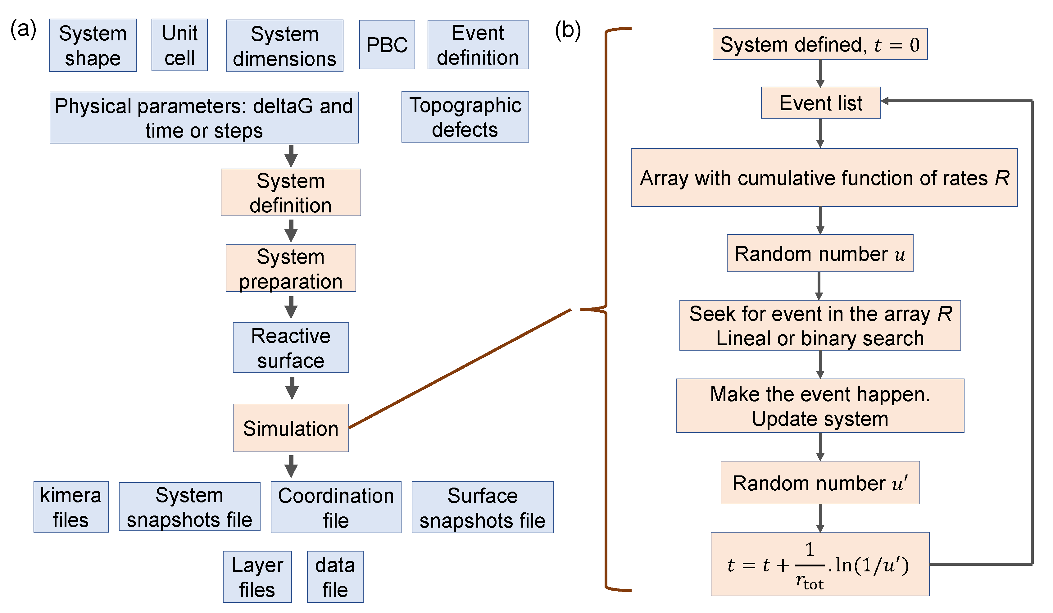
3.1. Operation

The workflow of the program can be differentiated in three parts (see Figure 1a):

3.1.1. System Definition

The user defines the essential parameters of the simulation in an input file. The order in which commands are given is relevant, as some instructions can overwrite previous ones, totally, or partially. In these cases KIMERA always takes into account the last command. Some important steps are:

• The mineral structure. The program can either read it from a standard ‘.xyz’ file, or can be defined by commands, or a combination of both. The ‘.xyz’ file [43] is easily obtained by tools such as VESTA [44] from downloadable ‘.cif’ files in mineralogical databases [45]. In principle KIMERA is thought to construct mineral surfaces replicating a small unit cell. Nevertheless, it is also possible to define a complex system within a ‘.xyz’ file and threat it as the whole system box. Coarse grained systems can be also simulated.
• The system dimensions. The program replicates the unit cell in the three spatial directions. Studies of different planes are possible by unit cell transformations with external programs such as VESTA [46]. KIMERA can apply periodic boundary conditions (PBC) in the three spatial directions.
• System shape. The program has commands to create different crystalline shapes of the system into complex surfaces or particles. For the moment the available geometries are cubic, spherical, parallelepiped, ellipsoidal, tick planes, or a combination of them.
• Topographic defects can be defined in the system, such as insoluble regions, dislocations, impurities and vacancies. There are two ways of defining impurities; it is possible to define them in the unit cell indicating their occupancy, or introducing them ex post once the system has been defined.
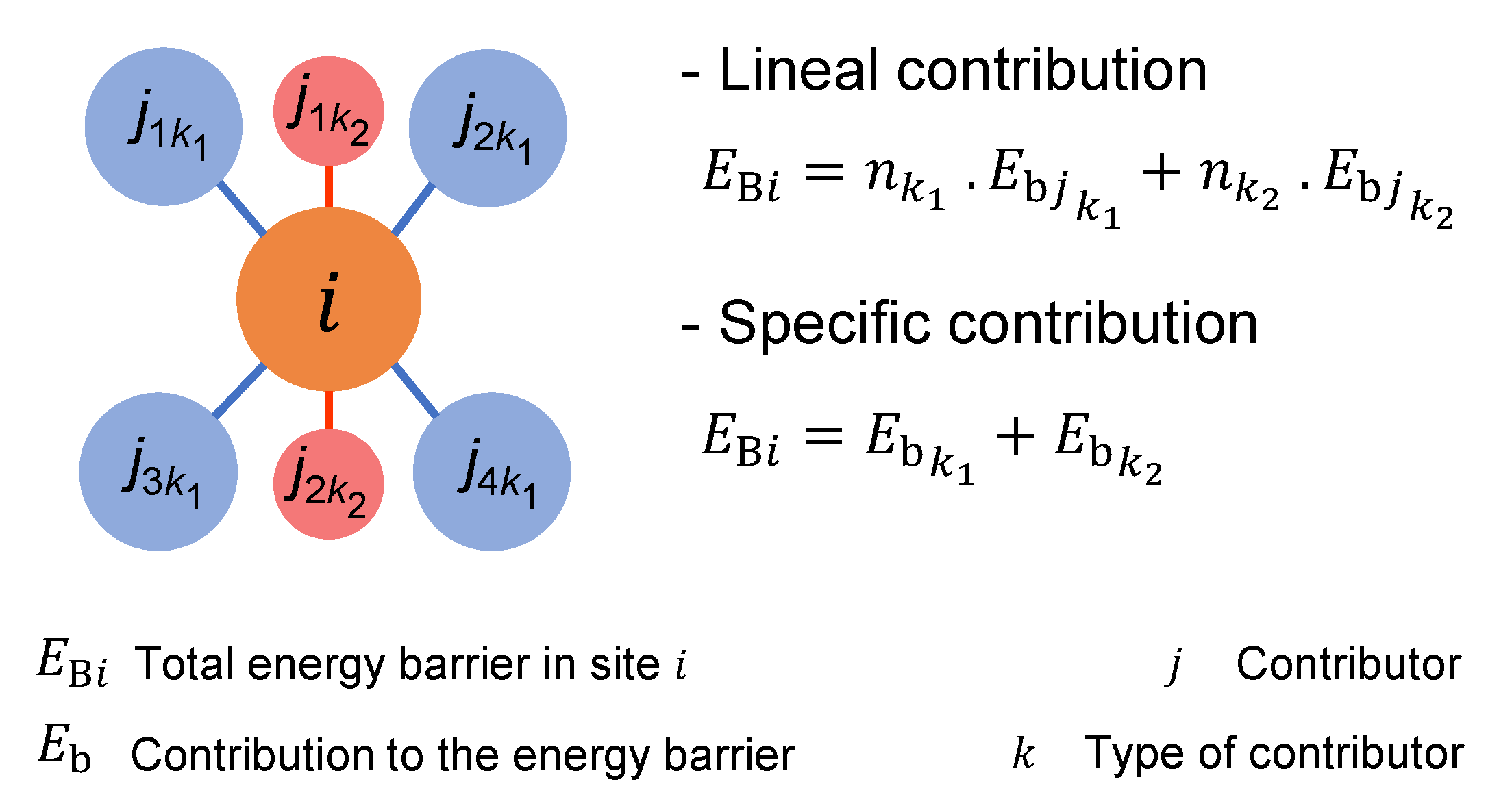
• Event definition. The KMC algorithm simulates the time evolution of a system as a set of possible events. These events take place at a rate that follows an Arrhenius equation (Equation (1)). A recent study demonstrates that the net dissolution of a mineral can be characterized using decoupled reactions of dissolution and precipitation [29]. Hence, we use that KMC scheme, so the fundamental frequency of the Arrhenius equation, f, splits into $f_{\mathrm{D}}$ or $f_{\mathrm{P}}$, and $E_{\mathrm{B}}$ into $E_{\mathrm{D}}$ or $E_{\mathrm{P}}$ depending if considering a dissolution or a precipitation event respectively. The energy barrier is characteristic of each chemical reaction and its neighbourhood, and can be obtained from the bibliography and/or ab initio calculations [22,23]. Supposing n neighbours of an atom, KIMERA can set $E_{\mathrm{D}}$ and $E_{\mathrm{P}}$ as a linear (Equation (6)) or a specific (Equation (7)) function of each neighbour j [23,47] (see Figure 2):

  $$E_{{\mathrm{D}}_k}=E_{\mathrm{d}}·n{E}_{{\mathrm{P}}_k}=E_{\mathrm{p}}·n$$

  (6)

  $$E_{{\mathrm{D}}_k}=f\left(j\right)E_{{\mathrm{P}}_k}=g\left(j\right)$$

  (7)
  Note that Equation (6) is a specific case of Equation (7). Moreover, since the contribution to the energy barrier can be determined for several types of neighbours, k represents each set of contributors with the same characteristics and $E_{{\mathrm{D}}_k}$ and $E_{{\mathrm{P}}_k}$ its contribution for dissolution and precipitation energy barrier respectively.

  $$E_{\mathrm{D}}=\sum _{k=1}^m{E}_{{\mathrm{D}}_k}{E}_{\mathrm{P}}=\sum _{k=1}^m{E}_{{\mathrm{P}}_k}$$

  (8)
  With these two ways of defining the energy barrier, two different approaches can be considered to describe the dissolution events:

  1

  A bond by bond description: Each linking bond breaks sequentially so that when an atom has no bonds left, it is released from the mineral.

  2

  A site by site description: All bonds reactions are unified in only one event, and each site dissolves with joint probability.

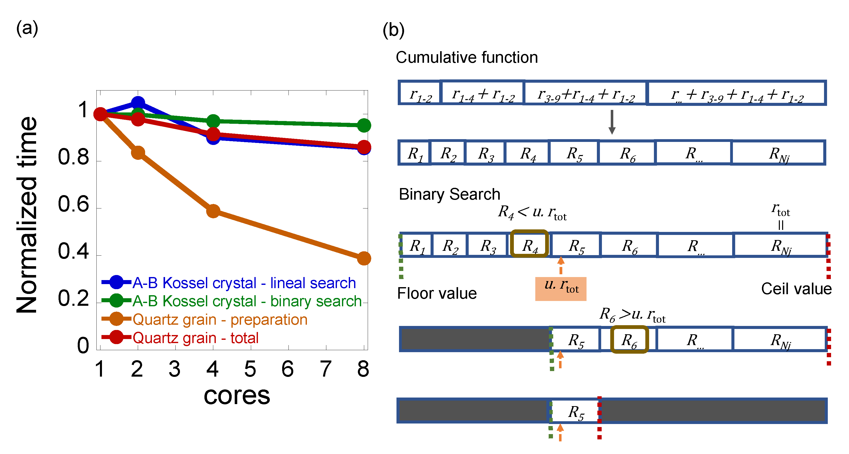
  As an additional element, KIMERA supports conditional event definition. Furthermore, it is possible to define the events based on ghost positions in the unit cell without physical meaning and to make a differentiation between atoms of the same type, for example it is possible to split the atoms of silica into Si1, Si2, etc. in the unit cell and then define events for each sub-element.
• Target time (s). Predicting the time scale beforehand in a complex system can be tough. There are two options for the simulation to finish. The simplest option is to indicate the number of simulation steps, that is, the number of events to accomplish. The other option is to specify the target time (s) until the simulation is going to run. The user can request the program to do an estimation of it by considering the initial possible events. Given s initial sorted groups of rates corresponding to atom removals with different coordination $r_1<r_2<\cdots <r_s$, the program approximates the total time for the system to dissolve as if all atoms $N_{\mathrm{a}}$ had the same rate value; the previous to the middle one.

  $$t_{\mathrm{approx}}=\frac{N_{\mathrm{a}}}{r_{\frac{s}{2}-1}}$$

  (9)
  This approximation arises from considering as limiting step the removal of the atom which leads to a kink atom, always with half of the mineral coordination [29,48].
• Optional parameters related with the output files. As we will see, output files contain information of the system time evolution like snapshots for visualization or the quantity of dissolved atoms.

3.1.2. System Preparation

Once KIMERA has read the input commands, taking into account the event definition and the PBC, it elaborates a list with all the neighbours for each atom. This step consumes a relatively large computational time, and KIMERA can use the output file from previous simulations as starting point to improve the performance. If restarting files are used, some previous commands have necessarily to be the same, but some commands can be changed to modify the simulation conditions. Most common changes are the values of $\Delta G$ or the energy barriers.

From the neighbour data, the program elaborates a list with the reactive initial surface. Nevertheless, the surface can be modified ad-hoc by the user via commands.

3.1.3. Simulation Process

A key step of the KMC algorithm is to find a random event from the list of possible events looking at its rate [39] (see Figure 1b). This step is the most time consuming. KIMERA has two possible ways to do the search. By default, the binary search method [49] is done. Briefly, it consists of successively dividing the search range in two and discarding the one without the wanted value (see Figure 3b). The other method is the common lineal search, which compares one by one all the values of the list. The relation between the computing time and the number of elements to compute N is named computational complexity O. The complexity of binary search is $O(log(N\left)\right)$. The complexity of lineal search is higher, $O\left(N\right)$, but it can be parallelized. Later we will discus the performance of both search methods in Section 3.2 and Figure 3a.

During the simulation, the output files generated by KIMERA are:

• Initial KIMERA file of the system in its own format (‘.initialkimerabox’). It is designed to save time in calculating neighbourhood, linked and affected atoms. A later simulation which reads this file will not need to do the preparation step.
• Final KIMERA file of the system (‘.finalkimerabox’). When the simulation has finished, or has encountered an error, the system is printed in KIMERA format.
• File with system snapshots (‘.box’) in LAMMPS format [33] for visualization. As this file can contain a lot of data, it may be better to handle the surface file unless for checking reasons.
• File with surface snapshots (‘.surface’) in LAMMPS format. Instead of the whole system, only the atoms on the surface are printed in this file.
• Data file with the time evolution of the following parameters (‘.data’): The total number of atoms dissolved of each type, its fraction, the surface dispersion, the gyradius (in no PBC systems) as well as all their derivatives.
• Coordination file with the mean coordination to each type of atom along the dissolution process (‘.meandiscoord’). This data is key to calculate correctly $\Delta G$ value as explained below.
• Layer atom files with the amount of atoms in each layer and each spatial direction (‘.alayer’, ‘.blayer’, ‘.clayer’). For example, the ‘.clayer’ file contains the total number of atoms of the cells in plane ab, layer by layer in c direction.

3.2. Parallelization Level

The parallelization level of a program is defined as the maximum speedup that a program can have. The speedup of a program from parallelization is limited by how much of the program can be parallelized [50]. For example, if 90% of the program can be parallelized, the theoretical maximum speedup using parallel computing would be 10 times no matter how many processors are used.

We have used the openMP library [42] to parallelize our code. As we have seen, the program presents three different parts: The system definition, the system preparation by KIMERA, and the simulation itself. The last two are the more time consuming and thus, they define the total simulation parallelization level. In Figure 3 the performance of the two first examples studied afterwards in Section 5 is plotted.

The preparation phase of the Kossel crystal example is very quick and hardly influences the total simulation time. Therefore it is a good example to get the parallelization level of the simulation phase. A decrease of $5\%$ by increasing the number of cores from 1 to 8 is obtained when using binary search. With lineal search the decrease is higher, $16\%$. Such difference is due to the former search method cannot be parallelized. While lineal search seems to be more efficient, the roles are expected to be swapped in simulations with bigger systems and low number of cores.

On the other hand, the quartz grain example needs a long system preparation time, which has been tracked separately. While the total time presents a reduction of $14\%$ with 8 cores, the system preparation phase shows a good parallelization level with a reduction of $61\%$. Therefore, best strategy to reduce the simulation time in a study with the same system is to use several cores to print only the initial Kimera file, to later used it in a set of subsequent simulations with only one processor and the default binary search.

4. Gibbs Free Energy Difference, $\Delta \mathbf{G}$

The Gibbs free energy difference $\Delta G$ is the driving force of a hydrolysis reaction in a mineral and it is related to the concentration of the chemical species of the mineral in the solvent. It is possible to obtain the dependence of the dissolution rate with Gibbs free energy in KMC simulations. The origin of this dependence has been demonstrated to reside at atomic scale and can be modeled by the interplay between dissolution and precipitation reactions, i.e., the microscopic reversibility [29]. The Gibbs free energy difference $\Delta G$ is related to the ion activity product, $\Pi$, of the dissolved material in water, divided by the solubility product $K_{\mathrm{s}}$:

$$\Delta G=R·T·ln\left(\Pi /K_{\mathrm{s}}\right)=R·T·ln\left(\beta \right)$$

(10)

R is the ideal gas constant ($8.3145$ J mol⁻¹ K⁻¹) and T the temperature (K). The term $\Pi /K_{\mathrm{s}}$ is more commonly known as saturation index $\beta$ and sets the distance to equilibrium, where no dissolution happens.

Due to concentration gradients, and accumulation of anions and cations in the Stern layer [51], there is a difference between macroscopic concentrations in solution and that close the surface. Therefore, we can define a “local” or microscopic free energy difference $\Delta G^{*}$:

$$\Delta G^{*}=R·T·ln\left({\beta }^{*}\right)$$

(11)

In principle, the dissolution will be driven by this microscopic free energy difference. The local and macroscopic $\Delta G$ can then be related by:

$$\Delta G=\Delta G^{*}-R·T·ln\left(\frac{{\beta }^{*}}{\beta }\right)$$

(12)

Numerically, we cannot establish a direct relationship between both quantities, because we do not know the microscopic saturation index ${\beta }^{*}$. However, we can relate them using the thermodynamic equilibrium condition and the dissolution and precipitation reaction rates. The thermodynamic equilibrium condition is define as the state when $\Delta G=0$. In that state, the net reaction rate must be also equal to zero, and therefore $r_{\mathrm{D}}=r_{\mathrm{P}}$. Using these conditions, together with Equations (4) and (5), we can obtain the following relationship for a monocomponent mineral:

$$\Delta G=\Delta G^{*}+\left(E_{{\mathrm{D}}_j}-E_{{\mathrm{P}}_j}\right)-ln\frac{f_{\mathrm{D}}}{f_{\mathrm{P}}}$$

(13)

In Equation (13) we assume that the total dissolution and precipitation rates correspond to those of the reaction step that limits the dissolution close to equilibrium, usually a kink site. In addition, if a multicomponent mineral is considered, the macroscopic $\Delta G$ is given by coupling the concentration of each constituent element [48]. The difference between the macroscopic and local free energies is implicitly taken into account in the $E_{\mathrm{D}}$ and $E_{\mathrm{P}}$ values. Supposing a mineral with l atoms types, m sets of contributor, and $n_k$ neighbours for each contributor set, the Gibbs free energy difference, $\Delta G$, is related with local $\Delta G^{*}$ by considering that the net dissolution rate of the kink atoms of each type (${\overline{n}}_k$ for all k) is 0 when $\Delta G=0$ ($k_{\mathrm{B}}T$ units):

$$\Delta G=\sum _{i=1}^l{\chi }_i·{\overline{N}}_i·\left(\Delta G^{*}+\left(\sum _{k=1}^m{E}_{{\mathrm{D}}_k}\left({\overline{n}}_k\right)-E_{{\mathrm{P}}_k}\left({\overline{n}}_k\right)\right)-ln\frac{f_{\mathrm{D}}}{f_{\mathrm{P}}}\right)$$

(14)

where ${\chi }_i$ is the fraction of atoms of type i, ${\overline{N}}_i$ is its average amount of broken bonds to dissolve, ${\overline{n}}_k$ is the average number of neighbours of each contributor set to the atom type i in a bond breakage or formation, and $E_{\mathrm{D}}\left({\overline{n}}_k\right)$ and $E_{\mathrm{P}}\left({\overline{n}}_k\right)$ are their respective energy barrier values. Both ${\chi }_i$ and ${\overline{n}}_k$ can be obtained from the output data of KIMERA, from the ‘.data’ and ‘.meandiscoord’ files respectively. Since these values can change with the considered $\Delta G^{*}$ value, the relation between $\Delta G^{*}$ and $\Delta G$ may not be constant. Nevertheless, in practice the deviation is not high and can be considered as constant by calculating them from simulation at far from equilibrium conditions, when $\Delta G^{*}\to -\infty$ and no precipitation events take place. The user must identify the value of ${\overline{N}}_i$ by recognising the number of broken bonds during a dissolution process. This differentiation arises for example if we want to group several bond breaking events in only one event of different f and $E_{\mathrm{B}}$, such as a coarse grain simulation. In the examples of the following section the $\Delta G$ calculus is explicitly highlighted.

5. Examples of KIMERA Capabilities

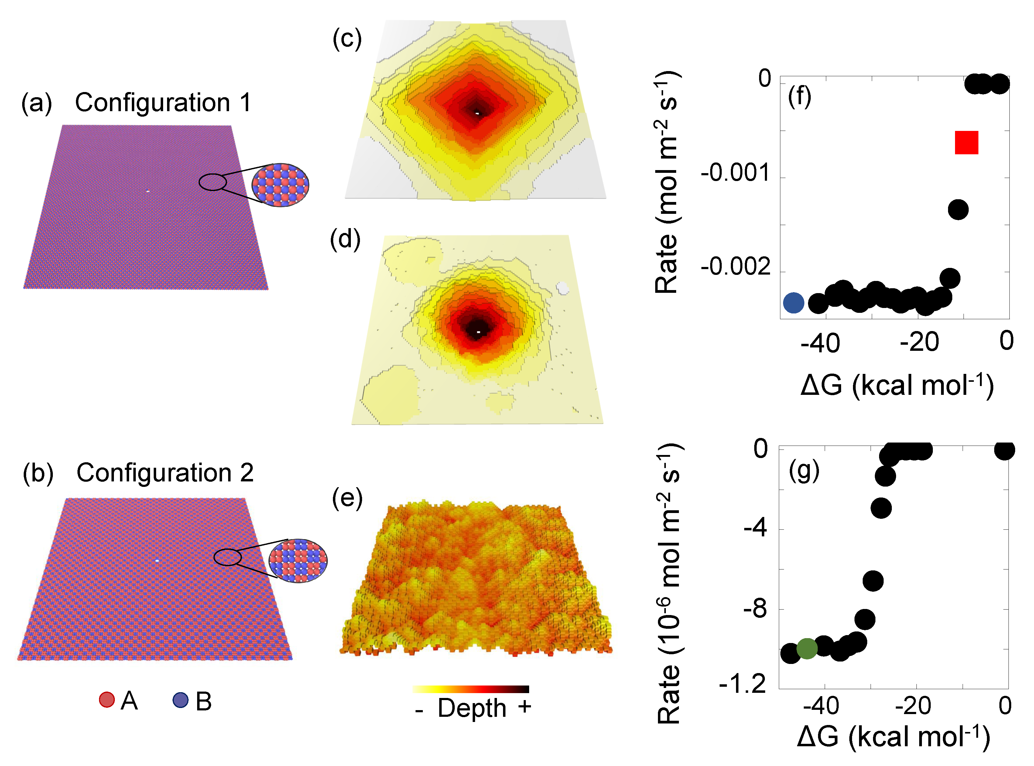
5.1. Model A-B Kossel Crystals

In this section the dissolution with $\Delta G$ of two different configurations of a Kossel crystal consisting of two elements is described. A Kossel crystal, or Terrace Ledge Kink system (TLK), is a simple mineral structure consisting of a cubic lattice with six first neighbours [52]. Despite the simplicity of this system, it ensures enough topographic details so as to reproduce the mechanisms attributed to the dissolution process.

The systems in this model have two elements, A and B. In one of them, named ‘configuration 1’, the atoms are distributed alternately along x and y axes (not in z) within a box of 120 × 120 × 30 atoms (see Figure 4a). In the other one, named ‘configuration 2’ groups of 2 × 2 × 2 atoms of the same element are distributed alternately along x, y and z axes (see Figure 4b). In both cases one dislocation of 2 × 2 atoms wide and 20 atoms depth is set in the center of the system. The dissolution study is done in the {001} plane using PBC.

Both cases are similarly defined. The simulation parameters for the ‘configuration 2’ are first described, and then the minor changes for the other case are indicated.

• The system dimensions are indicated; 60 × 60 × 15 unit cells.
• The unit cell parameters. We used $a=b=c=5$ Å and $\alpha =\beta =\gamma ={90}^{\circ }$. Inside the cell, we define the 8 positions of the atoms in the unit cell that later on is repeated along the system. The positions are: (0,0,0), (2.5,0,0), (0,0,2.5), (2.5,0,2.5), (0,2.5,0), (2.5,2.5,0), (0,2.5,2.5) and (2.5,2.5,2.5) Å. All the positions are initially define as A atoms, and we later will redefine half of them as B type. Note that although the unit cell has $5.0$ Å the distance between atoms is $2.5$ Å, which is a typical distance reported for minerals [54].
  In ‘configuration 1’, the positions are the same, but half of them are of type B. Specifically, atoms in (0,0,0), (0,0,2.5), (2.5,2.5,0) and (2.5,2.5,2.5) are B type. Since the alternating disposition of the atoms is already taken into account with this definition, no additional commands to modify the system are needed.
• We set periodic boundary conditions along x and y axes.
• Physical parameters for the simulation. The target time $t_{\mathrm{target}}=4.0·{10}^2$ s and the local $\Delta G^{*}=-100$ $k_{\mathrm{B}}T$ units, which ensures far from equilibrium conditions. In ‘configuration 1’ the time scale is different due to its faster dissolution and $t_{\mathrm{target}}=4.0·{10}^{-1}$ s.
• Event definition. We have chosen for this example an energy barrier for A-A atoms of $E_{{\mathrm{D}}_{\mathrm{A}-\mathrm{A}}}=12$ $k_{\mathrm{B}}T$ units, for B-B $E_{{\mathrm{D}}_{\mathrm{B}-\mathrm{B}}}=4$ $k_{\mathrm{B}}T$ units, which are respectively the higher and lower limit value for most minerals [27]. For the AB interaction the energy barrier is obtained from the Lorentz–Berthelot rule [55], $E_{{\mathrm{D}}_{\mathrm{A}-\mathrm{B}}}=\sqrt{E_{{\mathrm{D}}_{\mathrm{A}-\mathrm{A}}}·E_{{\mathrm{D}}_{\mathrm{B}-\mathrm{B}}}}=6.92$ $k_{\mathrm{B}}T$ units. The precipitation energy barrier for all the cases is $E_{{\mathrm{P}}_{\mathrm{A}-\mathrm{B}}}=E_{{\mathrm{P}}_{\mathrm{A}-\mathrm{A}}}=E_{{\mathrm{P}}_{\mathrm{B}-\mathrm{B}}}=1$ $k_{\mathrm{B}}T$ units.
  For the frequency $f_{\mathrm{D}}=f_{\mathrm{P}}=4·{10}^{13}$ s⁻¹ s which lies in the range of values for atomic vibration in a mineral (${10}^{10}$–${10}^{13}$ s⁻¹ at 300 K) [56].
  Lastly, KIMERA requires the number of neighbours that a bulk atom has to later define the initial reactive surface. For both for A and B atoms, a bulk atom has 3 A type neighbours and 3 B type neighbours. In ‘configuration 1’ the event definition is similar, but the number which defines a bulk atom changes. A bulk A atom has 2 A and 4 B neighbours. A bulk B atom has 4 A and 2 B neighbours.
• Topographic defects. We define the last plane $z=0$ as insoluble and we include one partial dislocation in the center with one third of the system depth. Since there are atoms within the dislocation that have a lower coordination than a bulk atom, the program recognised them as initial reactive surface. Therefore, we remove such condition because it is physically meaningless.

With those instructions KIMERA can start the simulations. Once the simulations are finished, we can relate $\Delta G^{*}$ and $\Delta G$ with Equation (14). The ‘.meandiscoord’ file reports the average bond breakage of each atom type during all the simulation. The final steady values are collected in

Table 1. Average bond breakage for each type of atom in the A-B Kossel crystal configurations and $\Delta G$ and $\Delta G^{*}$ relation.

	A-A	A-B	B-B	B-A	$\Delta \mathit{G}$
Configuration 1	1.0	1.33	1.0	2.66	$3·(\Delta G^{*}+18.76)$
Configuration 2	1.5	0.423	1.5	2.576	$3·(\Delta G^{*}+19.52)$

. Besides, the ‘.data’ files report the same dissolution rate for A and B atoms in both cases, thus ${\chi }_A={\chi }_B=0.5$. The relation between $\Delta G^{*}$ and $\Delta G$ is calculated from these values and Equation (14), and it is shown in Table 1. By changing the $\Delta G^{*}$ value, the dissolution rate versus $\Delta G$ is obtained in the Figure 4f,g from the slope of the number of atoms removed versus time normalized to the surface area (${(60·5.0·{10}^{-10})}^2=9·{10}^{-16}$ m²) and moles. Note that the rate may not be constant during the system dissolution. In ‘configuration 2’ the dissolution rate is constant with time since the dislocation has no effect. In contrast, in ‘configuration 1’ the dislocation opening provokes a progressive increase of the dissolution rate until dislocation coalescence. Thus we have taken the dissolution rate when it reaches the steady value after coalescence.

In ‘configuration 1’ the dislocation is not opened until enough energy is reached at $\Delta G=-9$ kcal mol⁻¹. The shape of the pit at this point is square (Figure 4c) but turns into a circular one (Figure 4d) with a small energy deviation. Besides, once the $\Delta G=-16.5$ kcal mol⁻¹ is reached, the spontaneous pit opening or mechanism III [29] is produced.

Regarding ‘configuration 2’, at close to equilibrium conditions only the very first B exposed atoms on the surface dissolve until only A atoms are exposed. The dissolution rate in this first zone is close to 0. Once the $\Delta G$ is negative enough at $-27$ kcal mol⁻¹ the release of A atoms starts and the dissolution rate increases drastically. It presents a random dissolution pattern over all the surface without any influence of the dislocation (see Figure 4e). The onset is only due to the beginning of the dissolution of the limiting A atoms. Note that, as expected, with the same $E_{\mathrm{D}}$ and $E_{\mathrm{P}}$ energies the dissolution rate is much lower in ‘configuration 2’ since groups of A atoms restrict it. Moreover the energy needed to activate its dissolution is much higher; the onset is at much lower $\Delta G$.

This type of theoretical examples on a Kossel crystal are very useful to study a general behaviour valid as a first approach for most minerals. However, as detailed below, more specific studies are possible in KIMERA.

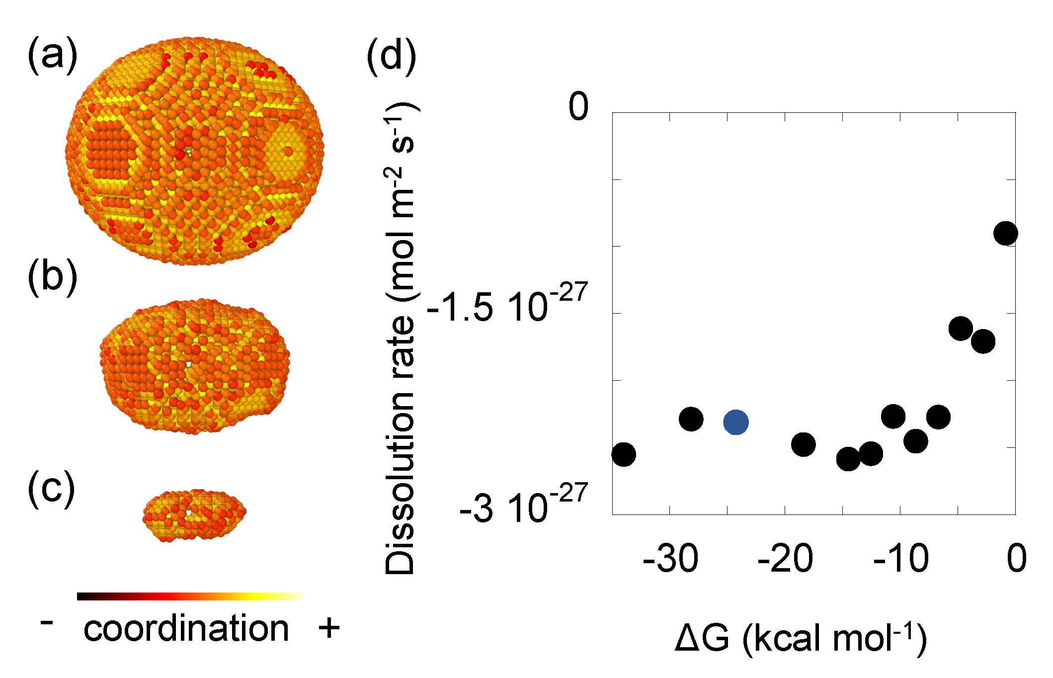
5.2. Quartz Model I: Dissolution of an Ellipsoidal Grain

KIMERA is able to simulate the dissolution of real minerals with full atomistic structure resolution. As example, we simulate the dissolution of an ellipsoid grain of quartz with $\Delta G$ using the SCS-L1 model described by Kurganskaya and Luttge [23]. Briefly, the SCS-L1 model proposed in [23] considers that the energy barrier for a silicon atom dissolution depends linearly with the amount of first surrounding silicon atoms $n_1$ and, to a lesser extend, with the second surrounding silicon atoms $n_2$ and hydroxils groups $n_3$ bonded to the surface.

$$E_{\mathrm{B}}=n_1·E_{{\mathrm{B}}_{\mathrm{Si}-\mathrm{Si}1}}+(n_2+n_3)·E_{{\mathrm{B}}_{\mathrm{Si}-\mathrm{Si}2}}$$

(15)

Note that $n_2+n_3=12$ in quartz. The specific energies are those proposed by [23]. Herein, we describe the instructions to run the simulation:

• System dimensions. A box in which we will define the ellipsoid is created with 50 × 40 × 30 unit cells.
• The unit cell parameters. For $\alpha$-quartz $a=b=5.01$, $c=5.47$, $\alpha =\beta ={90}^{\circ }$ and $\gamma ={120}^{\circ }$. Inside the cell, we load a ‘.xyz’ file containing the positions, which has been converted from a ‘.cif’ file downloaded from The American Mineralogist crystal structure database [45]. Oxygen atoms can be removed for performance purposes since they are not explicitly taken into account for the quartz dissolution reaction in this case. The dissolution of a SiO₂ is considered in a single step with a joint probability (Equation (6)). This can be interpreted as a coarse grain of a SiO₂ unit in each Si site.
• Physical parameters. The target time $t_{\mathrm{target}}=2.0·{10}^{20}$ s and the local $\Delta G^{*}=-100$ $k_{\mathrm{B}}T$ units.
• Topographic defects. An ellipsoid with radius in the three axes, $r_x=65$ Å, $r_y=85$ Å and $r_z=75$ Å is defined as the simulation system. A dislocation along the x axis is placed in the middle.
• Event definition. The energy barrier with first neighboring silicon atom is $E_{{\mathrm{D}}_{\mathrm{Si}-\mathrm{Si}1}}=28$ $k_{\mathrm{B}}T$ units and with second $E_{{\mathrm{D}}_{\mathrm{Si}-\mathrm{Si}2}}=4$ $k_{\mathrm{B}}T$. Precipitation energies of $E_{{\mathrm{P}}_{\mathrm{Si}-\mathrm{Si}1}}=10$ $k_{\mathrm{B}}T$ and $E_{{\mathrm{P}}_{\mathrm{Si}-\mathrm{Si}2}}=1$ $k_{\mathrm{B}}T$ are used. All the four first silicon neighbours are at 3.09832 Å. If an atom is surrounded by the four first neighbours, it is considered to be in bulk. 12 second silicon neighbours are at 5.01 Å. Finally, the fundamental frequencies values are $f_{\mathrm{D}}=f_{\mathrm{P}}=1.0·{10}^{12}$ s⁻¹ [57].

The relation between $\Delta G^{*}$ and $\Delta G$ is calculated using Equation (14) looking at the ‘.meandiscoord’ file to get the average breakage of atoms (see

Table 2. Average breakage value for each bond for the quartz grain example and $\Delta G^{*}$ and $\Delta G$ relation.

Si-Si-3.09832	Si-Si-5.0100	Si-Si-5.66774	Si-Si-4.42416	$\Delta \mathit{G}$
1.95	1.92	1.92	1.95	$1.95·(\Delta G^{*}+52.47)$

).

Figure 5 reports the dissolution rate versus $\Delta G$ and the time evolution of the grain, which is similar for all $\Delta G$ values. The grain dissolves maintaining an ellipsoidal shape with an irregular surface until its complete dissolution. The dissolution rate changes constantly as the exposed surface decreases. Therefore, we report the values when half of the forming atoms remains. The surface value is taken as a geometrical approximation in this point (see Figure 5b), $A_{1/2}=4·{10}^{-16}$ m².

The results show little influence of the dislocation in the dissolution rate. The local coordination at the dislocation does not decrease with respect to other grain regions, so it is not a preferential spot for dissolution. In this case the dissolution rate decreased gradually while getting close to equilibrium following a typical TST curve [56].

5.3. Quartz Model II: Dissolution of a Wulff Shape Particle

The previous quartz dissolution model is not able to reproduced jointly the experimental dissolution rate and activation energy [58]. If the dissolution parameters are fitted to reproduce the macroscopic activation energy, the dissolution rate is overestimated by several orders of magnitude, and vice versa. In this section we describe an example based on an alternative model proposed in [58]. In that work, in contrast to the previous site-by-site dissolution model, a bond-by-bond scheme is used, which is able to obtain both quantities along with the experimental topographies. The system is a wulff shape particle, the geometry with minimum surface energy of a mineral. For quartz it is a prism with hexagonal section and pyramidal tips [59] (see Figure 6a).

Instead of considering a coarse grain approximation where the quartz dissolves site by site, each oxygen bond breakage is explicitly considered. The energy barrier to break or reform the bond depends on its connectivity. We consider the connectivity by evaluating the number of unreacted oxygen atoms around the oxygen atom of interest. All of them are in a cutoff distance of $2.58\pm 0.01$ Å. If one hydrolysis reaction occurs in one of this neighbouring linking oxygen atoms, the bond breaks reducing the connectivity and, consequently, the energy barrier for the hydrolysis of the oxygen atom of interest. This way it can be defined the energy barrier for a hydrolysis as a function of the surrounding oxygen atoms in bridging sites (see

Table 3. Model energy barrier values with the bond surroundings in kJ mol⁻¹.

Bond	${\mathit{E}}_{\mathbf{D}}$	${\mathit{E}}_{\mathbf{P}}$	Surrounding Oxygen Atoms
Q1-Q1	-	-	0
Q1-Q2	75	60	1
Q1-Q3	85	70	2
Q1-Q4	95	80	3
Q2-Q2	85	70	2
Q2-Q3	95	80	3
Q2-Q4	105	105	4
Q3-Q3	105	105	4
Q3-Q4	135	135	5
Q4-Q4	-	-	6

).

• System dimensions. A box in which the wulff shape fit in is created with 16 × 16 × 47 units cells
• Same unit cell parameters as the previous example. $a=b=5.01$, $c=5.47$, $\alpha =\beta ={90}^{\circ }$ and $\gamma ={120}^{\circ }$. The ‘.xyz’ file is also called, but this time the oxygen atoms do play an important role and they cannot be removed.
• This time instead of target time, we define a target step $S_{\mathrm{target}}$ = 62,700 steps, which is approximately the total amount of silicon and oxygen atoms forming the particle.
• Topographic defects. The wulff shape is sculpted from the system by defining planes in which the atoms are removed. The equations of these planes are taken from GEODEBRA3D tool [60] which was used to visualise the system beforehand. Besides, two dislocations are defined and inner atoms removed from the initial surface. One dislocation is placed transversally in the center of the {100} plane, and another one perpendicular to the previous and longitudinally to the wulff shape
• Event definition. The $E_{\mathrm{D}}\left(n\right)$ and $E_{\mathrm{P}}\left(n\right)$ for the linking oxygen bond is directly related with the number of oxygen atoms within $2.585$ Å. 6 surrounding oxygen atoms indicates that the considered one is in a bulk position and therefore it is not reactive. Besides, the silicon atom must be automatically released if all of its four surrounding oxygen atoms have reacted. Finally, the fundamental frequency values $f_{\mathrm{D}}=f_{\mathrm{P}}=2.45·{10}^{10}$ s⁻¹ are indicated [61]. The $\Delta G^{*}=-200$ $k_{\mathrm{B}}T$ value sets very far from equilibrium conditions.

The next step is to determine the relation between $\Delta G^{*}$ and $\Delta G$. From the ‘.meandiscoord’ file, most oxygen atoms react when three oxygen atoms are around ($\overline{n}=3$). That means that the reference position to determine the $\Delta G$ value is a Q₁-Q₄ with $E_{\mathrm{D}}=24.1$ and $E_{\mathrm{P}}=20.3$$k_{\mathrm{B}}T$ units at 473 K (see Table 3). The relation between $\Delta G^{*}$ and $\Delta G$ is $\Delta G=\Delta G^{*}+3.8$.

It is important to highlight that in this process the number of broken bonds is ${\overline{N}}_i=1$, not like the previous model where the broken bonds corresponded to the number of surrounding silicon atoms.

Results of dissolution rate with $\Delta G$ is shown in Figure 6. They follow a typical TST curve. For all the simulations with $\Delta G$, initial wulff shape is distorted into an elongated grain which reduces its size until the complete extinction. Same as the previous model, dislocations do not represent a preferential spot for dissolution. The surface area and the dissolution rate values are calculated at the time when the grain has lost half of its atoms (see Figure 6b). The estimated surface area is $A_{1/2}=3.3·{10}^{-16}$ m².

6. Conclusions

In this paper we have introduced KIMERA, an open source KMC code to study mineral dissolution. The code offers portability thanks to its implementation in C++11 language and a good performance thanks to efficient algorithms and its parallelization feature. KIMERA is a versatile code thanks to the multiple ways to define reaction events, and the possibility of performing studies with specific atomistic structures, coarse grained systems, periodic systems or particles.

To illustrate it, three different models in four different systems are studied. First, a lineal dependence of the energy barrier of dissolution with the number of first neighbours is considered to study two different Kossel crystal systems. Second, a lineal dependence of the energy barrier with the number of first and second neighbours is considered to study the dissolution of an ellipsoidal grain of quartz. Finally, a specific dependence of the energy barrier with surroundings to represent the sequential breakage of bridging oxygen bonds is used to study the quartz wulff shape dissolution.

Future enhancements of KIMERA will include: (1) An improvement and widening of the event definition, to even consider a differentiation of $\Delta G^{*}$, $f_{\mathrm{D}}$ and $f_{\mathrm{P}}$ with positions, (2) an extension of the code to consider growth and (3) the development of a tool, webpage or IDE to create and display the system of study.

KIMERA is available as open-source software under the GNU General Public License. Thus, KIMERA can be used free of charge, everyone can contribute to the software, extend it to his own needs and share newly developed plug-ins with other users. The C++ source code of KIMERA, all input file examples, as well as the ‘.xyz’ needed for the quartz examples can be downloaded from the bitbucket repository https://mgp9999@bitbucket.org/mgp9999/kimera-publico.git.

References

- Van Breemen, N.; Buurman, P. Soil Formation; Springer: Berlin/Heidelberg, Germany, 2002. [Google Scholar]
- Kalbitz, K.; Solinger, S.; Park, J.H.; Michalzik, B.; Matzner, E. Controls on the dynamics of dissolved organic matter in soils: A review. Soil Sci. 2000, 165, 277–304. [Google Scholar] [CrossRef]
- Krouse, H.R.; Viau, C.A.; Eliuk, L.S.; Ueda, A.; Halas, S. Chemical and isotopic evidence of thermochemical sulphate reduction by light hydrocarbon gases in deep carbonate reservoirs. Nature 1988, 333, 415. [Google Scholar] [CrossRef]
- Canals, M.; Meunier, J.D. A model for porosity reduction in quartzite reservoirs by quartz cementation. Geochim. Cosmochim. Acta 1995, 59, 699–709. [Google Scholar] [CrossRef]
- Lal, R. Carbon sequestration. Philos. Trans. R. Soc. Lond. B Biol. Sci. 2008, 363, 815–830. [Google Scholar] [CrossRef] [PubMed]
- Lal, R. Soil Carbon Sequestration Impacts on Global Climate Change and Food Security. Science 2004, 304, 1623–1627. [Google Scholar] [CrossRef] [Green Version]
- Blain, S.; Quéguiner, B.; Armand, L.; Belviso, S.; Bombled, B.; Bopp, L.; Bowie, A.; Brunet, C.; Brussaard, C.; Carlotti, F.; et al. Effect of natural iron fertilization on carbon sequestration in the Southern Ocean. Nature 2007, 446, 1070. [Google Scholar] [CrossRef]
- Giammar, D.E.; Bruant, R.G., Jr.; Peters, C.A. Forsterite dissolution and magnesite precipitation at conditions relevant for deep saline aquifer storage and sequestration of carbon dioxide. Chem. Geol. 2005, 217, 257–276. [Google Scholar] [CrossRef]
- Juilland, P.; Gallucci, E. Morpho-topological investigation of the mechanisms and kinetic regimes of alite dissolution. Cem. Concr. Res. 2015, 76, 180–191. [Google Scholar] [CrossRef]
- Juilland, P.; Gallucci, E.; Flatt, R.; Scrivener, K. Dissolution theory applied to the induction period in alite hydration. Cem. Concr. Res. 2010, 40, 831–844. [Google Scholar] [CrossRef]
- Lasaga, A.C.; Blum, A.E. Surface chemistry, etch pits and mineral-water reactions. Geochim. Cosmochim. Acta 1986, 50, 2363–2379. [Google Scholar] [CrossRef]
- Brand, A.S.; Bullard, J.W. Dissolution kinetics of cubic tricalcium aluminate measured by digital holographic microscopy. Langmuir 2017, 33, 9645–9656. [Google Scholar] [CrossRef] [PubMed]
- Brand, A.S.; Feng, P.; Bullard, J.W. Calcite dissolution rate spectra measured by in situ digital holographic microscopy. Geochim. Cosmochim. Acta 2017, 213, 317–329. [Google Scholar] [CrossRef] [PubMed]
- Feng, P.; Brand, A.S.; Chen, L.; Bullard, J.W. In situ nanoscale observations of gypsum dissolution by digital holographic microscopy. Chem. Geol. 2017, 460, 25–36. [Google Scholar] [CrossRef] [PubMed]
- Cama, J.; Ganor, J.; Ayora, C.; Lasaga, C.A. Smectite dissolution kinetics at 80 °C and pH 8.8. Geochim. Cosmochim. Acta 2000, 64, 2701–2717. [Google Scholar] [CrossRef]
- Dove, P.M.; Han, N.; De Yoreo, J.J. Mechanisms of classical crystal growth theory explain quartz and silicate dissolution behavior. Proc. Natl. Acad. Sci. USA 2005, 102, 15357–15362. [Google Scholar] [CrossRef] [Green Version]
- Shvab, I.; Brochard, L.; Manzano, H.; Masoero, E. Precipitation mechanisms of mesoporous nanoparticle aggregates: Off-lattice, coarse-grained, kinetic simulations. Cryst. Growth Des. 2017, 17, 1316–1327. [Google Scholar] [CrossRef] [Green Version]
- Wang, Q.; Manzano, H.; Guo, Y.; Lopez-Arbeloa, I.; Shen, X. Hydration mechanism of reactive and passive dicalcium silicate polymorphs from molecular simulations. J. Phys. Chem. C 2015, 119, 19869–19875. [Google Scholar] [CrossRef]
- Wang, Q.; Manzano, H.; López-Arbeloa, I.; Shen, X. Water adsorption on the β-dicalcium silicate surface from DFT simulations. Minerals 2018, 8, 386. [Google Scholar] [CrossRef] [Green Version]
- Manzano, H.; Gartzia-Rivero, L.; Bañuelos, J.; López-Arbeloa, I.N. Ultraviolet–visible dual absorption by single BODIPY dye confined in LTL zeolite nanochannels. J. Phys. Chem. C 2013, 117, 13331–13336. [Google Scholar] [CrossRef]
- de Assis, T.A.; Reis, F.D.A. Dissolution of minerals with rough surfaces. Geochim. Cosmochim. Acta 2018, 228, 27–41. [Google Scholar] [CrossRef]
- Kurganskaya, I.; Luttge, A. Kinetic Monte Carlo approach to study carbonate dissolution. J. Phys. Chem. C 2016, 120, 6482–6492. [Google Scholar] [CrossRef]
- Kurganskaya, I.; Luttge, A. Kinetic Monte Carlo Simulations of Silicate Dissolution: Model Complexity and Parametrization. J. Phys. Chem. C 2013, 117, 24894–24906. [Google Scholar] [CrossRef]
- Rohlfs, R.D.; Fischer, C.; Kurganskaya, I.; Luttge, A. Crystal dissolution kinetics studied by a combination of Monte Carlo and Voronoi methods. Minerals 2018, 8, 133. [Google Scholar] [CrossRef] [Green Version]
- Briese, L.; Arvidson, R.S.; Luttge, A. The effect of crystal size variation on the rate of dissolution—A kinetic Monte Carlo study. Geochim. Cosmochim. Acta 2017, 212, 167–175. [Google Scholar] [CrossRef]
- Lasaga, A.C.; Luttge, A. Variation of crystal dissolution rate based on a dissolution stepwave model. Science 2001, 291, 2400–2404. [Google Scholar] [CrossRef]
- Meakin, P.; Rosso, K.M. Simple kinetic Monte Carlo models for dissolution pitting induced by crystal defects. J. Chem. Phys. 2008, 129. [Google Scholar] [CrossRef]
- Fischer, C.; Luttge, A. Pulsating dissolution of crystalline matter. Proc. Natl. Acad. Sci. USA 2018, 115, 897–902. [Google Scholar] [CrossRef] [Green Version]
- Martin, P.; Manzano, H.; Dolado, J.S. Mechanisms and Dynamics of Mineral Dissolution: A New Kinetic Monte Carlo Model. Adv. Theory Simul. 2019, 2, 1900114. [Google Scholar] [CrossRef] [Green Version]
- Artacho, E.; Anglada, E.; Diéguez, O.; Gale, J.D.; García, A.; Junquera, J.; Martin, R.M.; Ordejón, P.; Pruneda, J.M.; Sánchez-Portal, D.; et al. The SIESTA method; developments and applicability. J. Phys. Condens. Matter 2008, 20, 064208. [Google Scholar] [CrossRef]
- Gale, J.D. GULP: A computer program for the symmetry-adapted simulation of solids. J. Chem. Soc. Faraday Trans. 1997, 93, 629–637. [Google Scholar] [CrossRef]
- Giannozzi, P.; Andreussi, O.; Brumme, T.; Bunau, O.; Nardelli, M.B.; Calandra, M.; Car, R.; Cavazzoni, C.; Ceresoli, D.; Cococcioni, M.; et al. Advanced capabilities for materials modelling with Quantum ESPRESSO. J. Phys. Condens. Matter 2017, 29, 465901. [Google Scholar] [CrossRef] [PubMed] [Green Version]
- Plimpton, S. Fast Parallel Algorithms for Short-Range Molecular Dynamics; Technical Report; Sandia National Labs.: Albuquerque, NM, USA, 1993.
- Plimpton, S.; Thompson, A.; Slepoy, A. Stochastic Parallel PARticle Kinetic Simulator; Technical Report; Sandia National Laboratories: Albuquerque, NM, USA, 2008.
- Jørgensen, M.; Grönbeck, H. MonteCoffee: A programmable kinetic Monte Carlo framework. J. Chem. Phys. 2018, 149, 114101. [Google Scholar] [CrossRef] [PubMed] [Green Version]
- Hoffmann, M.J.; Matera, S.; Reuter, K. Kmos: A lattice kinetic Monte Carlo framework. Comput. Phys. Commun. 2014, 185, 2138–2150. [Google Scholar] [CrossRef] [Green Version]
- Holm, E.A.; Hoffmann, T.D.; Rollett, A.D.; Roberts, C.G. Particle-Assisted Abnormal Grain Growth; IOP Conference Series: Materials Science and Engineering; IOP Publishing: Risø, Denmark, 2015; Volume 89, p. 012005. [Google Scholar]
- Rodgers, T.M.; Madison, J.D.; Tikare, V.; Maguire, M.C. Predicting mesoscale microstructural evolution in electron beam welding. JOM 2016, 68, 1419–1426. [Google Scholar] [CrossRef] [Green Version]
- Jansen, A.P.J. An Introduction to Kinetic Monte Carlo Simulations of Surface Reactions; Springer: Berlin/Heidelberg, Germany, 2012; Volume 856. [Google Scholar]
- Bortz, A.B.; Kalos, M.H.; Lebowitz, J.L. A new algorithm for Monte Carlo simulation of Ising spin systems. J. Comput. Phys. 1975, 17, 10–18. [Google Scholar] [CrossRef]
- Dybeck, E.C.; Plaisance, C.P.; Neurock, M. Generalized temporal acceleration scheme for kinetic monte carlo simulations of surface catalytic processes by scaling the rates of fast reactions. J. Chem. Theory Comput. 2017, 13, 1525–1538. [Google Scholar] [CrossRef]
- Tian, X.; Bik, A.; Girkar, M.; Grey, P.; Saito, H.; Su, E. Intel® OpenMP C++/Fortran Compiler for Hyper-Threading Technology: Implementation and Performance. Intel Technol. J. 2002, 6, 36–46. [Google Scholar]
- Unofficial XYZ File Format Specification. Available online: http://en.wikipedia.org/wiki/XYZ_file_format (accessed on 1 October 2019).
- Momma, K.; Izumi, F. VESTA: A three-dimensional visualization system for electronic and structural analysis. J. Appl. Crystallogr. 2008, 41, 653–658. [Google Scholar] [CrossRef]
- Downs, R.T.; Hall-Wallace, M. The American Mineralogist crystal structure database. Am. Mineral. 2003, 88, 247–250. [Google Scholar]
- Unit Cell Rotation with VESTA. Available online: https://ma.issp.u-tokyo.ac.jp/en/app-post/1788 (accessed on 15 March 2020).
- Kohli, C.; Ives, M. Computer simulation of crystal dissolution morphology. J. Cryst. Growth 1972, 16, 123–130. [Google Scholar] [CrossRef]
- Lasaga, A.C.; Lüttge, A. Mineralogical approaches to fundamental crystal dissolution kinetics. Am. Mineral. 2004, 89, 527–540. [Google Scholar] [CrossRef]
- Williams, L.F., Jr. A modification to the half-interval search (binary search) method. In Proceedings of the 14th Annual Southeast Regional Conference, Birmingham, AL, USA, 22–24 April 1976; pp. 95–101. [Google Scholar]
- Hill, M.D.; Marty, M.R. Amdahl’s law in the multicore era. Computer 2008, 41, 33–38. [Google Scholar] [CrossRef] [Green Version]
- Dukhin, S.S.; Kretzschmar, G.; Miller, R. Dynamics of Adsorption at Liquid Interfaces: Theory, Experiment, Application; Elsevier: Amsterdam, The Netherlands, 1995. [Google Scholar]
- Oura, K.; Katayama, M.; Saranin, A.; Lifshits, V.; Zotov, A. Surface Science; Springer: Berlin/Heidelberg, Germany, 2003; Volume 602, pp. 229–233. [Google Scholar] [CrossRef]
- Stukowski, A. Visualization and analysis of atomistic simulation data with OVITO–the Open Visualization Tool. Model. Simul. Mater. Sci. Eng. 2010, 18, 015012. [Google Scholar] [CrossRef]
- Gibbs, G.V.; Downs, R.T.; Cox, D.F.; Ross, N.L.; Prewitt, C.T.; Rosso, K.M.; Lippmann, T.; Kirfel, A. Bonded interactions and the crystal chemistry of minerals: A review. Z. Krist. Cryst. Mater. 2008, 223, 1–40. [Google Scholar] [CrossRef]
- Berthelot, D. Sur le mélange des gaz. Compt. Rendus 1898, 126, 1703–1855. [Google Scholar]
- Lasaga, A.C. Kinetic Theory in the Earth Sciences; Princeton University Press: Princeton, NJ, USA, 2014. [Google Scholar]
- Pelmenschikov, A.; Leszczynski, J.; Pettersson, L.G. Mechanism of dissolution of neutral silica surfaces: Including effect of self-healing. J. Phys. Chem. A 2001, 105, 9528–9532. [Google Scholar] [CrossRef]
- Martin, P.; Gaitero, J.J.; Dolado, J.S.; Manzano, H. A Kinetic Monte Carlo Model for Quartz Dissolution. 2020; in preparation. [Google Scholar]
- Wendler, F.; Okamoto, A.; Blum, P. Phase-field modeling of epitaxial growth of polycrystalline quartz veins in hydrothermal experiments. Geofluids 2016, 16, 211–230. [Google Scholar] [CrossRef] [Green Version]
- Geodebra3d. Available online: https://www.geogebra.org/3d?lang=en (accessed on 15 March 2020).
- Casey, W.H.; Lasaga, A.C.; Gibbs, G. Mechanisms of silica dissolution as inferred from the kinetic isotope effect. Geochim. Cosmochim. Acta 1990, 54, 3369–3378. [Google Scholar] [CrossRef]