Article

pXRF Measurements on Soil Samples for the Exploration of an Antimony Deposit: Example from the Vendean Antimony District (France)

1
BRGM, F-45060 Orléans, France
2
Université du Maine, Géosciences, F-72000 Le Mans, France
3
CSTAT—Computational Statistics, Vienna University of Technology, 1040 Wien, Austria
4
GTK (Geological Survey of Finland), Environmental Solutions, 96101 Rovaniemi, Finland
*
Author to whom correspondence should be addressed.
Minerals 2020, 10(8), 724; https://doi.org/10.3390/min10080724
Submission received: 24 July 2020 / Accepted: 8 August 2020 / Published: 18 August 2020

Abstract

:
Mineral exploration is increasingly challenging in inhabited areas. To evaluate the potential of soil analysis by pXRF (portable X-ray fluorescence) as a low-footprint exploration technique, we revisited a historic Sb district in an agricultural area and performed shallow-soil sampling (Ah and B horizons) along profiles across known veins to capture the endogenic geochemical anomaly signals. Despite an expected bias between pXRF measurements and laboratory analyses, the former effectively located the Sb veins, especially when using their multi-element capabilities. Composition data processing (CoDa) and horizon-selective sampling significantly improved the method’s efficiency. On-site measurements allow dynamic sampling and mapping, helping with faster, cost-effective sample selection for further laboratory investigations. Based on this case study, where similar geochemical patterns were obtained for both horizons, application of an on-site approach to a humic horizon can increase survey efficiency and decrease impacts.

1. Introduction

For companies, the competitiveness of mineral exploration is based on reducing costs and capital intensity, improving dynamics and shortening delays between target testing and feasibility analysis. The exploration industry faces several constraints depending on the geographical location of projects, often developed far from infrastructure and analytical laboratories. Establishing field laboratories in remote areas and the shipping of samples involve significant logistics challenges and create data-transmission bottlenecks caused by distance between experts. While drill-core geochemistry for resource and reserve estimates for feasibility studies still requires traditional laboratory analysis as an essential step in regional exploration, commodity detection, target investigation and ranking can become significantly cheaper and quicker with the use of field analysers. This is because the goal is not the absolute accuracy of the measurements, but rather the relative ranking of the element concentrations and their anomaly to background contrast. Portable X-ray fluorescence (pXRF) technology allows dynamic decision-making and agile exploration management and facilitates cost-effective exploration [1].
Minimising sample preparation and shipping greatly reduces the environmental footprint of exploration. Case studies of pXRF applications on exploring different metals need to be presented to increase its acceptance.

1.1. Objectives

This study was carried out as part of the European EIT Raw Materials project UpDeep [2]. It is part of a demonstration of surface geochemical methods in southern European conditions, while similar studies are being carried out also in Finland and Greenland to demonstrate the applicability of the methods in northern Europe. Surface geochemistry is tested to provide means for geochemical exploration across Europe besides deep geochemistry [3,4]. The aim of surface geochemistry is to prioritise potential exploration targets by reducing time and cost while improving reliability in target detection. The key benefit is insignificant or non-existing environmental impact in the sampling phase that allows sampling in environmentally sensitive terrains. Low-footprint exploration strategies are necessary in Europe, where social acceptance of surface mining activities is particularly low.
Several methods based on wet chemistry are currently being tested, including partial-extraction soil analysis and plant analysis. Surface geochemical exploration is based on analysing trace amounts of metals or other elements and soil hydrocarbons in plants and soil horizons to discover deep-buried mineralisations. [3,4]. pXRF technology has been tested to greatly reduce impacts even further by diminishing sample shipping and the use of sample digestions. In addition, pXRF would also allow dynamic sampling design and on-site decision making of sample selection for further wet chemistry and survey orientation. To test the applicability of pXRF, two French sites were studied: the Echassières Li-Ta-Sn-W deposit [5] and the Les Brouzils Sb deposit (this study).
Antimony is considered a critical metal and is on the EU’s list of critical substances [6] due to its very high dependence (87% in 2017) on its import from China. Antimony is required for a variety of industrial materials such as flame-retardants, plastics, paint pigments, glassware and ceramics, ammunition alloys and batteries [7]. As a result, global Sb consumption has increased to more than 140 kt each year [8,9]. Its most promising use may be in producing rechargeable lithium-ion and sodium-ion batteries, since Sb-based materials are promising ultra-fast high-capacity anodes [10]. On the other hand, monitoring Sb concentrations in soils is also a key aspect of constraining its environmental and possible health [11] impact, in particular on former mining areas [12].
In this context, Sb is a desirable target commodity element for exploration companies. Syngenetic antimony deposits are known in young orogenic belts (Sedex or epithermal, [13]). The most important Sb deposits are orogenic veins of the slate-belt type, like Les Brouzils. In older belts, most Sb occurs as epizonal remobilisation through hydrothermal, fracture-bound circulations [14,15,16]. In such settings, the surficial footprint of mineralisation is usually elongated and thin (from 1 m to 50 m wide), while the irregular shape of orebodies makes them challenging targets for drilling. Trenching and soil surveys are, therefore, the traditional preferred exploration methods [17]. Reducing the footprint of high-density soil profiles and vegetation surveys is desirable. High-density soil sampling transects are required to detect the veins in addition to laboratory confirmation analyses on a subset of samples, usually selected on site. We try here to demonstrate how pXRF, definitely a low-footprint technique, can be effective for the precise delineation of Sb anomalies if adequate statistical treatment is applied.

1.2. Site and Geology

The study area (Figure 1) belongs to the Vendée antimony district located in western France, southeast of Brittany. The Vendée district has been known for a long time, with the first mention of mining activities on antimony ore deposits during the 18th century at La Ramée [18]. Operations started in the area during this period on several mineralised structures. At the beginning of the 19th century, the discovery of a rich vein at Rochetrejoux led to new activities until 1925. After the discovery of mineralised quartz during the 1950–1970s, the French Geological Survey (BRGM) conducted a stream-sediment geochemical survey [19] followed by soil sampling focusing on sediment anomalies, which led to the discovery of around 20 new prospects distributed on a 50 × 20 km area [18], in particular at Les Brouzils, La Télachère and La Copechagnière (Figure 1). Mining operations started again until the mid-1990s at the Les Brouzils mine.
The geological framework of the area is Variscan metamorphic rocks (gneiss and amphibolites) and slightly metamorphised sedimentary rocks. The western part of the Vendée Sb district is located on the northern side of the Chantonnay syncline. It is made of slightly metamorphised sedimentary rocks (sandstones, conglomerates and schists), locally crosscut by hectometric dolerite dykes. The edge of the syncline is affected by a regional-scale 120–140° N shear-zone, which is believed to be the structural control of the antimony deposits. Indeed, thrust and shear generated a network of conjugated tension fractures, controlling Sb mineralisations. The Copechagnière mineralised veins occur in the Les Essarts metamorphic complex, which comprises orthogneiss and paragneiss with high-pressure metamorphic relics, amphibolite derived from eclogite and banded amphibolite.
The Les Brouzils ore deposits consists of a principal lode system dipping at 70° towards the southeast.
It extends over at least 800 m horizontally and is recognised up to 100 m vertically [19]. It is a cataclastic zone 6–7 m thick, with a progressive transition towards host rocks. Brecciation intensively developed at the vicinity of the mylonites. Richer veins are localised at the border or the lode systems, but some satellite veins cement breccia elements. Distribution of mineralisation in the lode system is heterogeneous, and five richly mineralised columns were described, with horizontal extension of 30–120 m. The principal characteristic of this ore deposit is the presence of large blades of stibnite. Berthierite, pyrite and arsenopyrite complete the paragenesis. Formation of the deposit is polyphased, with vein infill from several successive hydrothermal episodes [21,22,23]. The Les Brouzils ore-deposit resources were estimated in the 1990s at 9250 t of metal Sb, with 4800 t of proven reserves with 7.5% ore [19].
In the La Télachère prospects, trenches and drill holes on the two principal anomalies determined the presence of a quartz lode system with associated stibnite. The best results in the area yielded 0.20 m at 9% Sb, and 0.30 m at 12.60% Sb. Paragenesis comprises stibnite, arsenopyrite, galena, sphalerite, berthierite, chalcopyrite, tetrahedrite and pyrrhotite in a quartz gangue. Gold was also observed. In La Télachère, several other Sb anomalies have not yet been investigated further.
In the southern part of the study area, near La Copechanière, two other vein systems were discovered by soil geochemistry and VLF (Very low frequency) investigations during the 1980s. They are subvertical quartz NW-SE veins with stibnite, and with a thickness of 0.2–0.3 m.
The entire area is partially covered by plateaux silts and gravels of mixed allochtonous (eolian) and autochtonous origin. Thickness of the plateau loess can be comprised in the range 0.5–2 m. Its age is assumed to be Würm [24].
Most of the geochemical patterns in soil are endogenic, driven by the underlying bedrock. The aeolian component behaves as a homogeneous dilutant. Soils in the area are well developed, with thickness often exceeding 1 m [25]. Weathering of underlying bedrock can lead to alteration profiles reaching 15 m thick. The typical profile starts, from top to bottom, with a relatively thin humic horizon (Ah, maximum 10 cm), passing to a thick horizon of clay accumulation (B, maximum 1.5 m) and a thick C horizon (up to 10 m).

2. Materials and Methods

2.1. Sampling

At the study area, 73 sampling points were spread over six profiles and three Sb prospects (Figure 2). After a first survey to observe typical soil profiles of the area, samples from Ah horizon were carefully collected after removing surficial vegetation and pebbles. The B horizon was sampled by hand auger at a constant 30 to 60 cm sampling depth (Figure 3).
Raw soil samples collected in the field (200–300 g) in dry conditions were carried in kraft paper bags closed with wire, and were received with some clay agglomerates. They were subsequently disaggregated and further air dried, and then sieved to 2 mm for removal of gravel and vegetation. A riffle splitter was used to prepare subsamples for pXRF and laboratory work. This ensured homogenisation through splitting. Soil material was placed in a Niton sample cup without a film cover, hand pressed and shot from above using a Niton mini-field stand.
Samples collected from Ah and B horizons were processed as independent data sets in order to assess the efficiency of the horizons for Sb exploration by identifying spatial anomaly patterns.
The sampling transects were designed to be perpendicular to the known mineralised structures (Figure 2). At the time of sampling, the Les Brouzils site was grassland. For La Télachère and La Copechagnière, northern profiles were cultivated (maize), whereas southern profiles are located in wild forest environments. To minimise possible anthropic contaminations, samples were collected at hedges between agricultural fields. The southern profiles were located in the forested woodland.

2.2. pXRF Analyses

To fit best the objectives of the project, the pXRF survey should have been conducted on-site during sampling. However, this was not possible for logistical reasons, so samples were analysed by pXRF in the laboratory one week after the campaign, using almost the same method as usually performed on-site (on-site sieving being performed without drying). This allowed simulation of the on-site selection of samples for laboratory analyses [1]. It is well-known [27,28,29,30] that moisture and sample preparation significantly affect raw pXRF measurements, and that a laboratory-type sample preparation offers results closer to laboratory analyses, but at the expense of a slower and more difficult workflow on the field. For the needs of our demonstration, it was chosen to perform measurements the same way as they would have been on site, i.e., on roughly homogenised samples without drying, and with moderate porosity reduction. No matrix-specific calibration was attempted. For the same reason, only the usual certified reference materials (CRMs) were used for quality monitoring, without the acquisition of matrix-matching CRMs, as would have been the case on-site.
Measurements were performed in soil mode with a Niton XL3t-980 pXRF spectrometer (Thermo Fischer, Billerica, MA, USA) and a lab stand. The spectrometer uses a 50-kV tube with an Ag anode, a large silicon drift detector (SDD) and a set of three filters. Soil mode (Compton) was used and counting time was 90 s (30 s per filter). Sb measurements are made using the Kα and Lα lines according to the instrument’s software. The LOD was defined as the 3σ standard deviation of the blank, and was reported for each sample according to its matrix composition.
Samples were analysed as air dried but not fully dry. The impact of residual moisture is limited under 20%, especially as linearity is more important than absolute accuracy.
The spectrometer’s built-in analysis program reports results for Ag, As, Au, Ba, Ca, Cd, Co, Cr, Cs, Cu, Fe, Hg, K, Mn, Mo, Ni, Pb, Pd, Rb, S, Sb, Sc, Se, Sn, Sr, Te, Th, Ti, U, V, W, Zn and Zr. Among these, Au, Hg, Pd and Te were not kept, as they are often affected by interferences, and because their distribution is too heterogeneous and prone to nugget effects in most samples. Some elements were found to be below the analytical limit of the spectrometer for most samples and do not appear in the Results Section 3.

2.3. QA/QC

Quality assurance (QA) and quality control (QC) were performed similar to any type of laboratory analysis, using blanks at regular intervals, certified reference materials (CRMs), internal standards and duplicates. QA/QC methods are fully applicable to pXRF [27].

2.4. Laboratory Analyses

Laboratory analyses were performed by ACME Bureau Veritas (Vancouver, BC, Canada) using the AQ250 method, which includes aqua regia digestion of 0.5 g of sample at 95 °C and ultra-trace analysis by ICP/AES (Inductively coupled plasma atomic emission spectroscopy) and ICP/MS (Inductively Coupled Plasma Mass Spectrometry) for Ag, Al, As, Au, B, Ba, Be, Bi, Ca, Cd, Ce, Co, Cr, Cs, Cu, Dy, Er, Eu, Fe, Ga, Gd, Ge, Hf, Hg, Ho, In, K, La, Li, Lu, Mg, Mn, Mo, Na, Nb, Nd, Ni, P, Pb, Pd, Pr, Pt, Rb, Re, S, Sb, Sc, Se, Sm, Sn, Sr, Ta, Tb, Te, Th, Ti, Tl, Tm, U, V, W, Y, Yb, Zn and Zr.
The aqua regia digestion method is not total, while pXRF is a total analysis technique. This may introduce biases for refractory elements [1,31]. The elements discussed in Section 3 are not refractory enough to lead to significant biases.

2.5. Data Processing

Classical statistical analysis requires that the data be normal or log-normal and represent one population. With typical geochemical data, the samples are compositions of chemical element contributions, and this interdependence already reflects that the relevant information is not contained in the absolute concentration values but rather in their (log-)ratios. Compositional data analysis (CoDa) [32,33] allows analysis of these log-ratios, and thus, the relative information rather than the absolute information.
Therefore, concentrations do not vary independently and should not be plotted in the Euclidean geometry. This is particularly true for pXRF analyses, which are multielement data, and include both major and trace elements. Element concentrations should, thus, be treated as relative information. Multivariate techniques such as PCA (Principal Component factor Analysis) and correlation analysis [32] are particularly affected by compositional data structure. Hence, absolute concentrations must be first opened by pairwise log ratios of transform techniques, such as the centred log ratio (clr) [33,34,35].
To avoid the biases mentioned by [33,34], the most significant variables and their correlations were not identified from correlation analysis on raw element concentrations, but were deduced from PCA (Principal Component factor Analysis) and CA (correspondence analysis). PCA was used to understand the relationships and possible dependencies between variables, while CA allowed us to understand the relationships between observations and variables. The Cochran C test was then used to identify the variables with an estimate of variance significantly larger than others. Statistics were provided by the XLSTAT package version 2019.3.2 (Addinsoft, Bordeaux, France), which offers most of the classical functions through an Excel add-on, and a window on R for more elaborate features. Further processing is currently being performed using R, with a dedicated interface currently being developed by the UpDeep project, which should allow processing in the field.

3. Results

3.1. Exploratory Data Analysis

Data analysis is conducted here with the pXRF results alone, in order to simulate what exploration geologists would do without laboratory results, the latter being used only for later quality assessment. Our objective is to make full use of the multi-element capabilities of the pXRF, which need no extra time or cost, rather than using it as a single-element analyser. Beyond this, we also wish to demonstrate the benefit of CoDa analysis of multielement data over raw data. Both raw and clr data sets were processed. It might seem that such data processing would affect the real time benefits of pXRF, but it can be achieved by mobile software in field conditions [2].
According to [33,34], the most significant variables and their correlations were identified by PCA (Principal Component factor Analysis) and CA (correspondence analysis) [35] on raw values first (Figures S1–S11 in Supplementary File), and then on clr-transformed values (Figure 4, Figure 5, Figure 6, Figure 7, Figure 8 and Figure 9 below). Among the 29 elements measured by pXRF (Ag, As, Ba, Ca, Cd, Co, Cr, Cs, Cu, Fe, K, Mn, Mo, Ni, Pb, Rb, S, Sb, Sc, Se, Sn, Sr, Th, Ti, U, V, W, Zn and Zr), nine elements (Ag, Cd, Co, Cs, Sc, Se, Sn, U and W) had no or little values above the lower analytical limit (LOD) reported by the instrument. Descriptive statistics for the other 20 elements are provided in Tables 1 and 3 for elements with over 20% measurements above LOD.
The accuracy of pXRF analyses is often debated because pXRF measurements on raw or roughly prepared loose samples often differ from laboratory analyses of the same samples. There are many possible reasons for discrepancies, apart from instrumental ones: a more thorough sample preparation in the laboratory, the use of a wet chemical analysis method instead of XRF and the type of digestion used. Comparisons should be based on pressed pellet XRF in the laboratory, but this is seldom used, and most laboratory work nowadays is based on ICP/AES and ICP/MS.
However, measurement data sets are consistent and usually exhibit quasi-linear relationships with laboratory analyses, provided that a total digestion method is used [1]. Censored data (under the LOD) were replaced by the maximum 3σ value reported by the instrument. This value is greater than the most probable value under the pXRF calibration, but is not necessarily an accurate value. The only important feature is that such values are consistent with the regular (>LOD) data. Element associations were investigated through the PCA and CA analyses. They were used to identify the elements carrying most of the variance in the data set. This was performed separately for the Ah and B data sets.

3.1.1. B Horizon

Samples from the B horizon (mineral subsoil) were usually collected at a depth of 30 to 60 cm. Descriptive statistics are provided in Table 1.
Pearson correlations on raw data (Figures S2 and S9 in Supplementary File) show no significant meaningful trend in connection with Sb and chalcophile elements, apart from Mn. Most trends observed are related with parent lithology. The data set was then converted to clr—centred log ratios [32]. The Pearson correlation matrix clearly separates one lithology-related group of elements (Rb, K, Ti, Sr, Th, Zr) and another mineralisation-related group of elements (Sb, As), which includes Mn and Fe in heat map format (Figure 4). A second group of elements (S, Pb, Ba) seems to be unrelated with (Sb, As, Mn) and closer to the lithology group.
The Cochran C test was then used to identify the variables with an estimate of variance significantly larger than others. Among these elements, only Sb, As and Mn show significant anomalies (Figure 5), and Fe is also controlled by lithology.
To reduce compositional data bias, we examined element relationships through PCA. The correlation matrix was used, 18 eigenvalues were calculated and graphs were selected from six eigenvectors. Rotation was not applied. An Sb-As-Mn association appears more clearly for Factor F3 (Figure 6 and Table 2).
A Pb-Ba association is noted for F5, but with less than 6.5% of total variance. Correspondence analysis (CA) was used to relate these associations with specific samples and possibly with mineralisation signatures or alteration phenomena.
The association between Sb and As is a major driver for F1 (Figure 7), while Mn is less clearly supported by F1 and appears clearly on F2. When reporting samples along these factors, samples BV0065 and BV0069 are highlighted, and sample BV0043 is opposed on F2. Samples BV0065 and BV0069 are high-Mn, with only BV0069 with high Sb, while sample BV0043 has low Mn and high Sb. The positive driver for F1 is a Zr-Th-K-Rb association, most likely related with lithology (heavy minerals, micas). BV0043 differs also by its contents in Ca, while all other samples are extremely depleted.

3.1.2. Ah Horizon

Samples from the Ah horizon (humic topsoil) were collected usually between 2–7 cm deep. Elementary statistics are provided in Table 3.
Pearson correlations on raw data are given in Figure 8. We observed Sb-As and Cu-Zn correlations separately.
We then examined element relationships through PCA. An Sb-As association appears more clearly (Table 4, Figure 8 and Figure 9). The Sb-Pb association is carried by factor F4 (Table 4). S is in relation with both groups.
The Pearson correlation matrix clearly separates one lithology-related group of elements (Rb, K, Ti, Sr, Th, Zr) and one mineralisation-related group of elements (Sb, As, Mn, Figure 10), which includes Fe in heat map format (Figure 8). The lithology-related group of elements (Rb, K, Ti, Sr, Th, Zr, Pb) also includes Pb in the heat-map format, and the mineralisation-related group of elements includes Ca and Fe in this format (Sb, As, Mn, Fe, Ca), suggesting that Ca and Fe are controlled at least partly by mineralisation processes. Among the elements, As, Sb and Mn show significant anomalies (Figure 9), as do Ba and Ca.

3.1.3. Variations Between Ah and B Horizons

The concentration ranges do not differ significantly between B and Ah horizons (Table 2 and Table 3). Differences in geochemical behaviour are observed in the geochemical signatures (Section 3.1.1 and Section 3.1.2) and spatial distribution (Section 3.2). Variations were, therefore, analysed as ratios and enrichment factors (Figure 11). Average and median values were similar between B and Ah for As, Cr, Cu, K, Mn, Rb and Ti. Higher values were observed in the B horizon for Ba, Fe, Sb, V and Zr compared to the Ah horizon. Lower values were observed for Ca, Pb, S and Zn. Sb and As seem to display a moderate depletion in the Ah horizon (Figure 11).

3.2. Spatial Anomaly Mapping

To better understand the possible benefits of pXRF soil surveys in exploration, samples from the Ah and B horizons were processed and mapped as independent data sets. Maps were also drawn using PCA and CA factor scores for samples. They do not show much more information than single-element maps, but might be useful for other data sets.
On the element maps (Figure 12, Figure 13, Figure 14, Figure 15, Figure 16 and Figure 17), the classes boundaries for each element were selected according to quantiles. Unlike distribution breaks, this allows the lower values of each element’s concentration to be put forward in order to show low-level anomalies best.

3.2.1. Sb Spatial Anomaly Patterns

The profiles sampled in the three areas illustrated in Figure 2 are shown in Figure 10, Figure 11, Figure 12, Figure 13, Figure 14, Figure 15 and Figure 16, separately for the horizons Ah and B.
In the La Télachère area, a moderate but conspicuous Sb anomaly was observed both on Ah (Figure 12) and B (Figure 13) data, with higher Sb concentrations in the latter. A similar pattern was observed for As (Figure 14 and Figure 15), while the Mn anomaly was weaker, which was mainly observable in the topsoil (Figure 16) and slightly shifted to the east.
In La Copéchagnière, the Sb anomaly was weak, close to the LOD of the pXRF instrument. It would require a careful comparison with laboratory analyses to determine whether Sb variations by pXRF are meaningful or not, and properly located. We observed arsenic anomalies in the B horizon, but they are less obvious in the Ah horizon. A weak Mn signal was observed in the Ah horizon data.
The most prominent anomalies were observed in the Les Brouzils area near the abandoned mine works. Sb anomalies were located near the expected position of the quartz-Sb vein on both profiles, in both horizons (Figure 12 and Figure 13). The distance to reported mineralisation was no more than 50 m. Additional single sample anomalies were observed further away, but their position near roads or tracks might be related to the past mining activity.

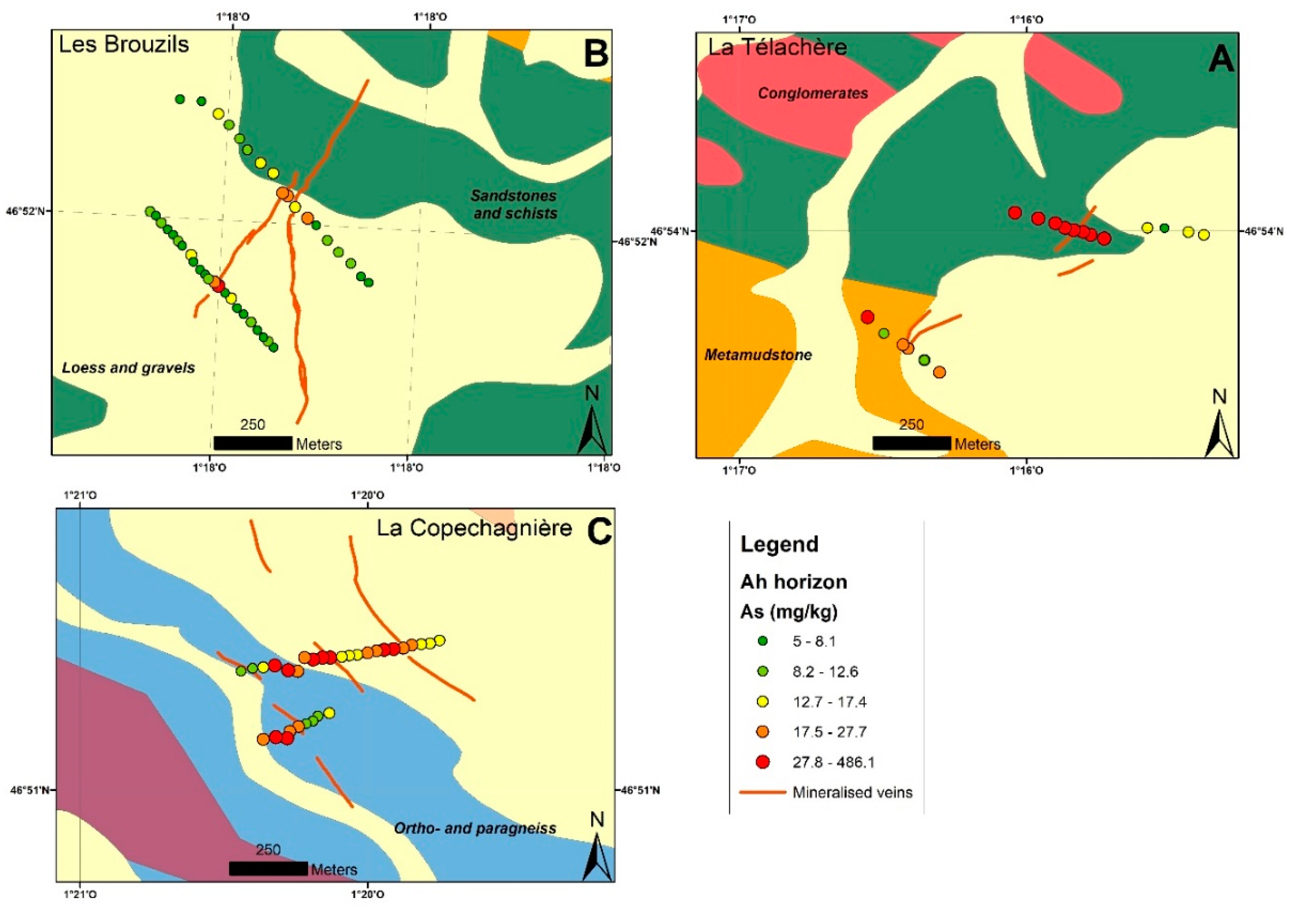
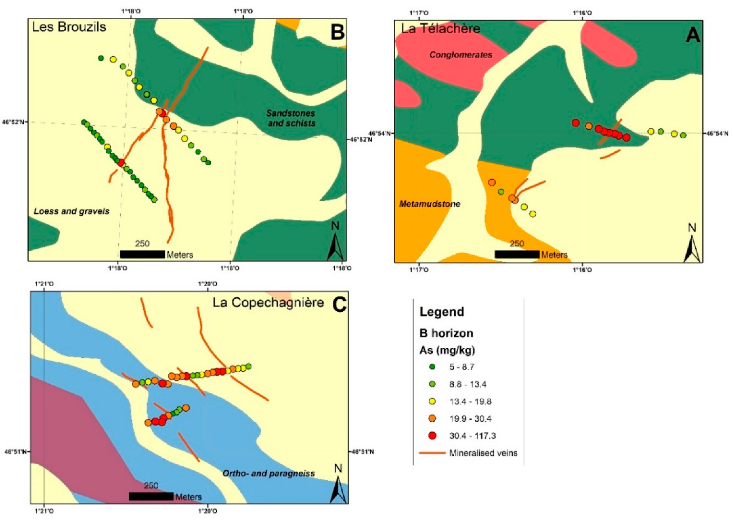
3.2.2. As Spatial Anomaly Patterns

Sharp anomalies were observed in the Les Brouzils area, south profile; La Télachère, north profile; and la Copechagnière, north profile. Weaker As anomalies are observable on the other profiles, especially on the B horizon (Figure 14 and Figure 15). Similar to Sb, the distance to reported mineralisation was no more than 50 m.

3.2.3. Mn Spatial Anomaly Patterns

The anomalies for Mn are observed on a slightly wider area (Figure 16 and Figure 17), though still centred on known mineralisation, with a slight drift towards the southeast. This may reflect the larger contrast between Mn’s lower analytical limit and observed Mn concentrations. Sb has more intense gradients than Mn along the profiles.
Maps drawn with PCA factor scores (Figure 18) did not bring a significant advantage. They are similar to Mn maps, but represent the La Télachère orebody better.

3.3. Quality Control

3.3.1. pXRF QA/QC

On the basis of regular pXRF measurements of CRMs, all reported elements showed satisfactory agreement for at least one CRM (Table 5). Discrepancies may reflect matrix incompatibility. Blank sample measurements are satisfactory.
To assess reproducibility, triplicate measurements were made on a subset, shooting on slightly different locations (Table 6). Thus, the reproducibility also includes the sample heterogeneity. This explains higher (10 to 20%) variation rates for As, Sb, S, Cr, Mo, Ni and V, which are controlled by mineralised grains. Variability is less than 10% for the other elements.

3.3.2. pXRF Quality Control by Laboratory Analyses

Usually, external control of pXRF measurements is performed on a subset of the analysed samples by submitting this subset to an external laboratory analysis, operating under its own QA/QC scheme [27]. It would be ideal to perform this by comparing pXRF results with laboratory XRF analyses to avoid possible biases related to digestion. This was not possible within the budget and time frame, but the comparison of pXRF measurements with aqua regia ICP/AES and ICP/MS analyses provided confirmation of consistency and LODs. This was possible because the main elements under investigation (Sb, As, Mn, Pb and Zn, see the Exploratory data analysis section) are readily soluble in aqua regia for the mineral paragenesis observed. Another possible source for discrepancies lies in sample preparation, as pXRF measurements were carried on dried and sieved but not milled soil samples, instead of lab-ready pulps. This was chosen to better simulate on-site measurements.
Although laboratory analyses were performed on lab-ready pulps after aqua regia digestion, and our measurements were on dried raw samples, an acceptable linear correlation was observed (Figure 19, and similar patterns for Mn and Zn). Both Sb and As showed a positive bias for pXRF (27 and 14%), which did not affect sample ranking.
Overestimation for Sb and As cannot be caused by porosity. Underestimation due to partial dissolution by aqua regia is possible, but unlikely, because most Sb and As minerals are not refractory. In other projects, negative bias for these elements may be observed. We believe that standard calibration in soil mode is not optimal for Sb below 200 mg/kg. One possible explanation is that the factory calibration and standards did not closely match the samples’ ranges. Having a custom calibration with matching standards, or better, with spiked SRMs from the same matrix, might improve this bias, but would need repeated measurements. We did not investigate this in detail, as the ranking of the samples was not affected. The bias for As, combined with good linearity (R2 = 0.955), is acceptable for exploration. Good correlations were also observed for Mn and Zn, with minor bias (−5% and +3%).

4. Discussion

4.1. CoDa Processing

Raw data processing results are less efficient than clr data processing results, demonstrating that CoDa interpretation is more efficient. Raw data are what the geochemist will see while sampling and analysing. CoDa processing may seem complex but can be performed on the same day or the next, using an ordinary laptop. On-site selection and dynamic sampling are still possible as the geochemist is still on site.

4.2. Soil Horizons

No systematic variations were observed between horizons Ah and B, apart from Ca and Ba. Variations of Sb and pathfinder elements (As, Mn) are of the same order of magnitude. Arsenic anomalies observed in the B horizon are less obvious than in the Ah horizon. The weak Mn signal in the Ah horizon is shifted, and thus, we suspect that it reflects surficial enrichment.
The strong Ca enrichment in the Ah horizon (Figure 11) may reflect pedogenetic processes or lime addition for agricultural practices in acid soils. Ba enrichment could not be explained.

4.3. Spatial Anomaly Mapping

The richer profiles at area B (Les Brouzils) showed small but conspicuous Sb anomalies (Figure 12 and Figure 13), while area A (La Télachère) and area C (La Copéchagnière) profiles showed weaker anomalies. Using a lower concentration profile for Sb at area A (La Télachère) improved the resolution, despite the poor absolute accuracy, as the numbers were very close to the LOD.
Using quantiles, Sb classes boundaries were selected preferentially in the lower range of the element concentration, in order to show better low-level anomalies (Figure 12 and Figure 13).
It seems that Mn anomalies are less sharp, from a spatial point of view, or more diffuse than Sb or As anomalies. Mn is known for scavenging Sb during Sb mobility under reducing conditions [36]. However, this does not explain the spatial distribution of Mn. Other possibilities would be an earlier Mn deposition during mineralisation events, or a wider diffusion of Mn in the vein selvages due to higher mobility.

4.4. Application to Exploration

We were able, using pXRF measurements, to detect shallow Sb mineralisation based on single-element Sb patterns, but this did not give positive results for all occurrences. The mineralisation was missed at the La Télachère south profile and the La Copechagnière north profile. Detection was improved using Sb and pathfinder elements (As, Mn) patterns where single-element Sb patterns failed. At least one pathfinder could be detected at profiles where Sb was not detected. Threshold values can be estimated for these elements (As: 30 mg/kg, Mn: 400 mg/kg). The larger contrast between the lower Mn analytical limit and observed Mn concentrations makes Mn a more sensitive pathfinder than As. We cannot provide mineralogical evidence for ore-forming or hydrothermal processes explaining this, as we did not have access to any vein outcrop or to historic drill cores, but the association is confirmed statistically and spatially. It is not often cited [36,37] and it might be related to the aptitude of Mn hydroxides to scavenge Sb by changing its redox state [12,38]. However, this is not applicable to geochemical dispersion under surface conditions, as the cartographic distribution of Mn is linked with vein position. It is more likely that Mn was part of the mineralising event, either by deposition or by selvage alteration.
We did not attempt deeper ore detection from soil profiles, as previous prospection did not target deeper ore. The profiles we tested were set across known anomalies and were too short to have a chance to cross other anomalies. Longer profiles or grid patterns would be needed.
On the Les Brouzils mineral occurrences, soil anomalies appeared no further than 50 m from the known position of antimony veins. Single-sample anomalies were observed further away, but their position near roads or tracks might be caused by the past mining activity.
The representativeness of pXRF data alone is satisfactory according to two criteria:
-
Ranking samples according to Sb and pathfinder concentrations, as a linear relationship is observed between pXRF measurements and laboratory analyses, even with a bias affecting absolute accuracy.
-
Delineating precise anomalies, as the spatial consistency of anomalies with known mineralisation location is good.
Beyond the absolute accuracy issues, exploration decisions based on the pXRF geochemical data set are reliable, in terms of the dynamic sampling plan. Sampling uncertainties and matrix heterogeneity issues in laboratory analyses can be reduced by using multiple measurements by pXRF on site, prior to shipping, allowing optimised sample selection.
This selection can be based on pXRF results due to linearity [1,39]. Decisions with financial consequences, such as drilling programs or detailed investigations, will require this laboratory confirmation. However, decisions on further reconnaissance investigations, such as higher density sampling or area extensions, can be made on the basis of pXRF measurements and geology alone.
The lower accuracy of field analyses is compensated for by the much larger number of analyses made possible by on-site methods. An added benefit of pXRF analyses is the quantified uncertainty for each sample, allowing direct integration into geostatistics.
More detailed multielement processing based on the CoDa toolbox has yet to be completed in the UpDeep project. It may be tested later on promising structures without known mineralisation.
The B horizon is generally the preferred medium target for geochemical exploration, as it concentrates most indicator elements. Similar geochemical contrasts between the B and humic horizon (Ah) have already been demonstrated [40]. Earlier, [41] demonstrated that it could also be representative of the C horizon. For the Vendée case study, our results agree well with these statements. Ah can be sampled quickly and easily.

5. Conclusions: Prospecting for Sb with a pXRF

This work contributes to evaluating whether pXRF is an effective tool for focusing investigations at the early stage, defining geochemical patterns and allowing fast vectorisation based on quasi-real time measurements. It also allows for the more effective selection of samples for laboratory analyses, focusing on critical samples and reducing the number of routine ones. Further benefits would be more efficient field campaigns and reducing sampling and drilling needs in Sb exploration. To achieve that, data quality are ensured by denser measurements and by QA/QC monitoring.
Samples were lain densely (10 to 30 m) on predefined profiles, so narrow and shallow veins were located effectively. It would have been beneficial to further reduce the spacing between sampling points. From multielement pXRF measurements, we conclude that:
-
Based on single-element Sb patterns, mineralisation can often be detected, but not for all intercepts.
-
Based on Sb, As and Mn patterns, Sb mineralisation can be detected using pathfinders. A composite signature search (Sb, As, Mn) turned out to be more effective for mineralisation detection than single Sb maps. The pathfinder signature needs to be determined prior to the survey. Maps drawn with PCA factor scores did not bring a significant advantage, but this may be due to the rather simple signature and to the lack of lithogeochemical influence. Factor-score maps might be useful at other sites.
-
Sb, As and Mn contrast is good, but the background values are not much above the lower analytical limit of the instrument on raw samples.
-
Using the same signature (Sb, As, Mn) for deeper ore detection is theoretically possible but more difficult. Based on the thickness of the surficial cover and on the structural control, a weaker signal could be expected.
-
Detection of weak anomalies may be hampered by background noise and scatter. No demonstration was made on the site, as previous prospection did not target the deeper ore.
Portable XRF measurements on soil samples from carefully selected horizons Ah and B provide relevant information while exploring for vein-type or structure-hosted antimony mineralisations. The low cost and fast execution of pXRF measurements allow high spatial density on profiles or grids, therefore reducing the potential uncertainty of the significance of measurements close to the lower analytical limit.
The execution of pXRF profiles by auger does not require heavy field work and may be conducted at high spatial density. In terms of footprint, analysing soil for selected horizons is similar to the collection of surficial pedological samples. It is easily accepted by landowners and farmers, as it causes very limited damage to the vegetation cover. This damage can be further minimised by careful sampling procedures with cover restoration, and by focusing on the Ah horizon. Analyses with portable XRF of the Ah horizon are a cost-effective and efficient method to target such Sb ore deposits.
It might look difficult to conduct multivariate analysis or result mapping using GIS (Geographic information systems) while on site, but the computing capabilities of laptops, tablets and even smartphones are now sufficient to allow proper data interpretation on site, within minutes. The objective of the UpDeep project [2] is to provide a high level of data integration and processing, in a smooth and robust way, in order to overcome limitations on interpretation.
Elemental signatures and spatial patterns can be determined while sampling and can be used for planning further sampling points. The immediate availability of results allows sampling plans, profiles and grids to be refined according to observed anomalies. This approach, based on dynamic workplans [42] and adaptive sampling (ASAP) strategies [43], is both time- and cost-effective at the early stages. The main limitation is determining absolute concentrations, which may need time-consuming sample preparation or matrix-specific calibration to reduce bias, but bias does not affect spatial patterns or anomaly detection, which are the primary objectives of a survey.
Due to the relatively low cost of pXRF measurements, much higher density sampling is possible than for laboratory analyses, resulting in higher quality data sets [44]. On-site soil analyses by pXRF are effective for outlining anomalies, creating maps and locating mineralisation. However, the analyses need careful confirmation in the laboratory, such as anomaly ranking and deposit pre-evaluation before exploration moves to the next stage.
Field methods provide invaluable help for laboratory sample selection and screening. They improve the cost-effectiveness of analytical programs. Field methods help to control the representativeness of laboratory samples, for instance by assessing heterogeneity by multiple shots while sampling. The availability of a large field data set reduces the risk of overlooking sampling and preparation uncertainties with laboratory results.
The Vendée case study highlights that the humic horizon can increase efficiency of the survey and decrease its impacts, with faster access to the sample.

Supplementary Materials

The following are available online at https://www.mdpi.com/2075-163X/10/8/724/s1, Figure S1: pXRF measurements with over 20% observations above LOD, B horizon soils (pXRF, in mg/kg), Figure S2: Pearson correlations on pXRF raw data for B horizon soils (as heat map). The use of colour shading and its interpretation is described in [1], Figure S3: Contribution of each element to the 6 main factors for B horizon observations, pXRF raw data. Coloured cells indicate meaningful positive contributions, Figure S4: PCA factor diagrams for F1, F2 (a) and F3 (b). Samples from B horizon, pXRF raw data, Figure S5: CA symmetric plots for F1, F2 (a) and F3 (b). Samples from B horizon, pXRF raw data, Figure S6: Pearson correlations on clr data for B horizon Group B observations, pXRF measurements. The use of colour shading and its interpretation is described in [1], Figure S7: Cochran’s C test. Samples from B horizon, pXRF data. The C test detects one exceptionally large variance value at a time, Figure S8: Elementary statistics for Ah horizon observations, pXRF measurements (in mg/kg), Figure S9: Pearson correlations on raw data for Ah horizon, pXRF raw measurements (as heat map). The use of colour shading and its interpretation is described in [1], Figure S10: Contribution of each element to the 6 main factors for Ah horizon, pXRF measurements. Coloured cells indicate meaningful positive contributions, Figure S11: PCA factor diagrams for F1, F2 (a) and F3 (b). Samples from group Ah, pXRF raw data.

Author Contributions

Conceptualization methodology and validation, B.L. and J.M.; sampling, V.D., E.G., L.B.; investigation, P.A., V.D.; data curation, B.L., D.M., P.F.; writing—original draft preparation, review and editing, B.L., J.M., P.F., M.M.; visualization, J.M.; supervision and project administration, J.M., M.M. All authors have read and agreed to the published version of the manuscript.

Funding

This research is part of an upscaling project UpDeep, Upscaling deep buried geochemical exploration techniques into European business, funded by the European EIT Raw Materials. This activity received funding from the European Institute of Innovation and Technology (EIT), a body of the European Union, under the Horizon 2020, the EU Framework Programme for Research and Innovation.

Acknowledgments

Karen M. Tkaczyk, professional editor, proofread the manuscript and checked the language.

Conflicts of Interest

The authors declare no conflict of interest.

References

  1. Lemiere, B. A review of pXRF (field portable X-ray fluorescence) applications for applied geochemistry. J. Geochem. Explor. 2018, 188, 350–363. [Google Scholar] [CrossRef] [Green Version]
  2. Middleton, M.S.; Nykänen, V.; Melleton, J.; Lemiere, B.; Sarala, P.; Filzmoser, P.; Järvinen, P.; Rinkkala, M.; Rönnqvist, J.; Thaarup, S. Upscaling deep buried geochemical exploration techniques into European business—UpDeep. In Proceedings of the Resources for Future Generations—RFG2018, Vancouver, BC, Canada, 16–21 June 2018; p. 1227. [Google Scholar]
  3. Cameron, E.M.; Hamilton, S.M.; Leybourne, M.I.; Hall, G.E.M.; McClenaghan, M.B. Finding deeply buried deposits using geochemistry. Geochem. Explor. Environ. Anal. 2004, 4, 7–32. [Google Scholar] [CrossRef]
  4. Heberlein, D.; Dunn, C. Sweat, Sap And Emanations—What Trees and Snow Can Reveal About Hidden Mineralization. In Proceedings of the Resources for Future Generations—RFG2018, Vancouver, BC, Canada, 16–21 June 2018; p. 1941. [Google Scholar]
  5. Melleton, J.; Lemière, B.; Derycke, V.; Serrand, A.S.; Fournier, E.; Gloaguen, E.; Lacquement, F.; Auger, P.; Middleton, M.; Nykänen, V. Exploration geochemistry: Comparison between classic trace elements geochemistry, soil partial leaches, portable XRF, on soils and biogeochemistry in Western Europe Environment. Example from Li-Ta-Sn and W deposits. In Proceedings of the Resources for Future Generations—RFG2018, Vancouver, BC, Canada, 16–21 June 2018; p. 1395. [Google Scholar]
  6. European Commission. Communication from the Commission to the European Parliament, the Council, the European Economic and Social Committee and the Committee of the Regions Tackling the Challenges in Commodity Markets and on Raw Materials (COM/2011/0025 Final). 2011. Available online: https://eur-lex.europa.eu/legal-content/EN/TXT/?uri=CELEX:52011DC0025 (accessed on 20 December 2018).
  7. USGS 2015 Minerals Yearbook—Antimony. Available online: https://minerals.usgs.gov/minerals/pubs/commodity/antimony/myb1-2015-antim.pdf (accessed on 20 December 2018).
  8. Guo, X.; Wu, Z.; He, M.; Meng, X.; Jin, X.; Qiu, N.; Zhang, J. Adsorption of antimony onto iron oxyhydroxides: Adsportion behavior and surface structure. J. Hazard. Mater. 2014, 276, 339–345. [Google Scholar] [CrossRef]
  9. Henckens, M.L.C.M.; Driessen, P.P.J.; Worrell, E. How can we adapt to geological scarcity of antimony? Investigation of antimony’s substitutability and of other measures to achieve a sustainable use. Resour. Conserv. Recycl. 2016, 108, 54–62. [Google Scholar] [CrossRef]
  10. He, J.; Wei, Y.; Zhai, T.; Li, H. Antimony-based materials as promising anodes for rechargeable lithium-ion and sodium-ion batteries. Mater. Chem. Front. 2018, 3, 437–455. [Google Scholar] [CrossRef]
  11. ATSDR, Public Health Statement for Antimony, in Toxic Substances Portal. Available online: https://www.atsdr.cdc.gov/phs/phs.asp?id=330&tid=58 (accessed on 31 January 2020).
  12. Herath, I.; Vithanage, M.; Bundschuh, J. Antimony as a global dilemma: Geochemistry, mobility, fate and transport. Environ. Pollut. 2017, 545–559. [Google Scholar] [CrossRef] [PubMed]
  13. Pohl, W. Economic Geology: Principles and Practice: Metals, Minerals, Coal and Hydrocarbons—Introduction to Formation and Sustainable Exploitation of Mineral Deposits; Wiley-Blackwell: Chichester, UK, 2011. [Google Scholar]
  14. Munoz, M.; Courjault-Rade, P.; Tollon, F. The massive stibnite veins of the French Palaeozoic basement: A metallogenic marker of Late Variscan brittle extension. Terra Nova 2007. [Google Scholar] [CrossRef]
  15. Pochon, A.; Gloaguen, E.; Branquet, Y.; Poujol, M.; Ruffet, G.; Boiron, M.C.; Boulvais, P.; Gumiaux, C.; Cagnard, F.; Gouazou, F.; et al. Variscan Sb-Au mineralization in Central Brittany (France): A new metallogenic model derived from the Le Semnon district. Ore Geol. Rev. 2018, 97, 109–142. [Google Scholar] [CrossRef]
  16. Scratch, R.B.; Watson, G.P.; Kerrich, R.; Hutchinson, R.W. Fracture-controlled antimony-quartz mineralization, Lake George Deposit, New Brunswick; mineralogy, geochemistry, alteration, and hydrothermal regimes. Econ. Geol. 1984, 79, 1159–1186. [Google Scholar] [CrossRef]
  17. Sainsbury, C.L. Geochemical exploration for antimony in southeastern Alaska. USGS Open-File Rep. 1955, 55–158. [Google Scholar] [CrossRef]
  18. Marcoux, E.; Serment, R.; Allon, A. Les gites d’antimoine de Vendée (Massif armoricain, France); historique des recherches et synthèse métallogénique. Chron. Rech. Min. 1984, 476, 3–30. [Google Scholar]
  19. Le Fur, Y.; Allon, A.; Biron, R.; Lequertier, M.; Roussel, M. La découverte du gisement d’antimoine des Brouzils en Vendée (Massif Armoricain, France). Historique des travaux, description du gisement et projet d’exploitation. Chron. Rech. Min. 1988, 492, 5–18. [Google Scholar]
  20. Godard, G.; Bouton, P.; Poncet, D.; Carlier, G.; Chevallier, M. Geological Map 1:50,000, Montaigu; BRGM Editions: Orleans, France, 2007; p. 536. [Google Scholar]
  21. Bailly, L.; Bouchot, V.; Beny, C.; Milesi, J.-P. Fluid inclusion study of stibnite using infrared microscopy: An example from the Brouzils antimony deposit (Vendee, Armorican massif, France). Econ. Geol. 2000, 95, 221–226. [Google Scholar] [CrossRef]
  22. Pochon, A.; Gapais, D.; Gloaguen, E.; Gumiaux, C.; Branquet, Y.; Cagnard, F.; Martelet, G. Antimony deposits in the Variscan Armorican belt, a link with mafic intrusives? Terra Nova 2016, 28, 138–145. [Google Scholar] [CrossRef]
  23. Pochon, A.; Branquet, Y.; Gloaguen, E.; Ruffet, G.; Poujol, M.; Boulvais, P.; Gumiaux, C.; Cagnard, F.; Baele, J.-M.; Kéré, I.; et al. A Sb ± Au mineralizing peak at 360 Ma in the Variscan belt, BSGF. Earth Sci. Bull. 2019, 190, 4. [Google Scholar] [CrossRef] [Green Version]
  24. Ters, M. Action morphologique des phénomènes périglaciaires dans la region littorale vendéenne. Bull. Assoc. Géogr. Fr. 1953, 232–233, 78–87. [Google Scholar] [CrossRef] [Green Version]
  25. INRA. Base de Données Géographique des Sols de France à 1/1,000,000. 1998. Available online: www.gissol.fr (accessed on 24 July 2020).
  26. Béchennec, F. Carte Géologique Harmonisée du Département de Loire-Atlantique. BRGM Report RP-55703-FR. 2007. 369p. Available online: http://infoterre.brgm.fr/rapports/RP-55703-FR.pdf (accessed on 18 August 2020).
  27. Hall, G.; Buchar, A.; Bonham-Carter, G. Quality Control Assessment of Portable XRF Analysers: Development of Standard Operating Procedures, Performance on Variable Media and Recommended Uses. Canadian Mining Industry Research Organization (Camiro) Exploration Division, Project 10E01 Phase I Report. 2012. Available online: https://www.appliedgeochemists.org/index.php/publications/other-publications/2-uncategorised/106-portable-xrf-for-the-exploration-and-mining-industry (accessed on 24 July 2020).
  28. Gray, A. Form, Distribution, and Genesis of Precious Metal Mineralization within the Bald Hill Antimony Deposit, South-Central New Brunswick, Canada. Master’s Thesis, University of New Brunswick, Fredericton and Saint John, NB, Canada, 2019. [Google Scholar]
  29. Bastos, R.O.; Melquiades, F.L.; Biasi, G.E.V. Correction for the effect of soil moisture on in situ XRF analysis using low-energy background. X-Ray Spectrom. 2012, 41, 304–307. [Google Scholar] [CrossRef]
  30. Ge, L.; Lai, W.; Lin, Y. Influence of and correction for moisture in rocks, soils and sediments on in situ XRF analysis. X-Ray Spectrom 2005, 34, 28–34. [Google Scholar] [CrossRef]
  31. Caporale, A.G.; Adamo, P.; Capozzi, F.; Langella, G.; Terribile, F.; Vingiani, S. Monitoring metal pollution in soils using portable-XRF and conventional laboratory-based techniques: Evaluation of the performance and limitations according to metal properties and sources. Sci. Total Environ. 2018, 643, 516–526. [Google Scholar] [CrossRef]
  32. Aitchison, J. The Statistical Analysis of Compositional Data. Monographs on Statistics and Applied Probability; Chapman & Hall Ltd.: London, UK, 1986; p. 416. [Google Scholar]
  33. Filzmoser, P.; Hron, K.; Reimann, C. The bivariate statistical analysis of environmental (compositional) data. Sci. Total Environ. 2010, 408, 4230–4238. [Google Scholar] [CrossRef]
  34. Filzmoser, P.; Hron, K.; Reimann, C.; Garrett, R. Robust factor analysis for compositional data. Comput. Geosci. 2009, 35, 1854–1861. [Google Scholar] [CrossRef] [Green Version]
  35. Reimann, C.; Filzmoser, P.; Hronc, K.; Kynčlová, P.; Garrett, R.G. A new method for correlation analysis of compositional (environmental) data—A worked example. Sci. Total Environ. 2017, 607–608, 965–971. [Google Scholar] [CrossRef]
  36. Nicholson, K. Contrasting mineralogical-geochemical signatures of manganese oxides; guides to metallogenesis. Econ. Geol. 1992, 87, 1253–1264. [Google Scholar] [CrossRef]
  37. Ashley, P.M.; Craw, D.; Graham, B.P.; Chappell, D.A. Environmental mobility of antimony around mesothermal stibnite deposits, New South Wales, Australia and southern New Zealand. J. Geochem. Explor. 2003, 7, 1–14. [Google Scholar] [CrossRef]
  38. Belzile, N.; Chen, Y.; Wang, Z. Oxidation of antimony(III) by amorphous iron and manganese oxyhydroxides. Chem. Geol. 2001, 174, 379–387. [Google Scholar] [CrossRef]
  39. Young, K.E.; Evans, C.A.; Hodges, K.V.; Bleacher, J.E.; Graff, T.G. A review of the handheld X-ray fluorescence spectrometer as a tool for field geologic investigations on Earth and in planetary surface exploration. Appl. Geochem. 2016, 72, 77–87. [Google Scholar] [CrossRef] [Green Version]
  40. Cook, S.J.; Dunn, C.E. Final report on Results of the Cordilleran Geochemistry Project: A comparative assessment of soil geochemical methods for detecting buried mineral deposits. Geosci. BC Pap. 2007, 7, 225. [Google Scholar]
  41. Baker, B.E. An application of soil humix substances to geochemical exploration. Appl. Geochem. 1986, 2, 307–310. [Google Scholar] [CrossRef]
  42. Robbat, J.R.A. Dynamic Workplans and Field Analytics: The Keys to Cost-Effective Site Investigations; Case Study; Tufts University: Medford, MA, USA, 1997. [Google Scholar]
  43. US Department of Energy. Adaptive Sampling and Analysis Programs (ASAPs); Report DOE/EM-0592; US Department of Energy: Washingon, DC, USA, 2001.
  44. Ramsey, M.H.; Boon, K.A. Can in situ geochemical measurements be more fit-for-purpose than those made ex situ? Appl. Geochem. 2012, 27, 969–976. [Google Scholar] [CrossRef]
Figure 1. Geological map of the study area (modified from the geological maps at 1/50,000 scale of the Vendée district, [20]). The study areas are: A: La Télachère. B: Les Brouzils, C: La Copechagnière. Size of insert map is 1000 × 1000 km.
Minerals 10 00724 g001
Figure 2. Map of sample locations on geological background map [26]. (A): La Télachère; (B): Les Brouzils; (C): La Copechagnière.
Minerals 10 00724 g002
Figure 3. Flow chart showing sample collection and sample preparation.
Minerals 10 00724 g003
Figure 4. Pearson correlations on clr data for B horizon Group B observations, pXRF measurements. The use of colour shading and its interpretation is described in [35].
Minerals 10 00724 g004
Figure 5. Cochran’s C test. Samples from B horizon, pXRF data. The C test detects one exceptionally large variance value at a time.
Minerals 10 00724 g005
Figure 6. PCA factor diagrams for F1-F2 (a) and F1-F3 (b). Samples from B horizon, pXRF clr data.
Minerals 10 00724 g006
Figure 7. CA symmetric plots for F1-F2 (a) and F1-F3 (b). Samples from B horizon, pXRF clr data.
Minerals 10 00724 g007
Figure 8. Pearson correlations on clr data for Group Ah, pXRF measurements (as heat map). The use of colour shading and its interpretation is described in [35].
Minerals 10 00724 g008
Figure 9. Cochran’s C test. Samples from Ah horizon, pXRF raw data.
Minerals 10 00724 g009
Figure 10. PCA factor diagrams for F1-F2 (a) and F1-F3 (b). Samples from group Ah, pXRF clr data.
Minerals 10 00724 g010
Figure 11. B vs. Ah enrichment factors by element (B concentration/Ah concentration, averaged pXRF raw data for all points).
Minerals 10 00724 g011
Figure 12. Sb map of Ah horizon samples, (pXRF measurements in mg/kg). (A): La Télachère; (B): Les Brouzils; (C): La Copechagnière.
Minerals 10 00724 g012
Figure 13. Sb map of B horizon samples (pXRF measurements in mg/kg). (A): La Télachère; (B): Les Brouzils; (C): La Copechagnière.
Minerals 10 00724 g013
Figure 14. As map of Ah horizon samples (pXRF measurements in mg/kg). (A): La Télachère; (B): Les Brouzils; (C): La Copechagnière.
Minerals 10 00724 g014
Figure 15. As map of B horizon samples (pXRF measurements in mg/kg). (A): La Télachère; (B): Les Brouzils; (C): La Copechagnière.
Minerals 10 00724 g015
Figure 16. Mn map of Ah horizon samples (pXRF measurements in mg/kg). (A): La Télachère; (B): Les Brouzils; (C): La Copechagnière.
Minerals 10 00724 g016
Figure 17. Mn map of B horizon samples (pXRF measurements in mg/kg). (A): La Télachère; (B): Les Brouzils; (C): La Copechagnière.
Minerals 10 00724 g017
Figure 18. PCA F3 map of B horizon samples (pXRF measurements in mg/kg). (A): La Télachère; (B): Les Brouzils; (C): La Copechagnière.
Minerals 10 00724 g018
Figure 19. pXRF measurements vs. ICP/AES analyses, Ah horizon soils, in mg/kg: (a) Sb; (b) As.
Minerals 10 00724 g019
Table 1. pXRF measurements with over 20% observations above LOD, B horizon soils (pXRF, in mg/kg).
MeasurementsAsBaCaCrCuFeKMnMoNi
number7996966027969687175
min813595828215188926668746
max1174979471986649,07722,6654177971
avg283062696462820,36715,440474757
med193072180432719,51715,048386749
MeasurementsPbRbSSbSrThTiVZnZr
number9696133969496949296
min942 1949548525311181
max329387951513415918417067433
avg2067 10781956379327310
med2067 5279956138924302
Table 2. Contribution of each element to the six main factors for B horizon observations, pXRF clr data.
ContributionF1F2F3F4F5F6
As0.273−0.1470.3891−0.141−0.1160.035
Ba0.2860.070−0.168−0.019−0.177−0.402
Ca0.206−0.312−0.254−0.1280.1520.446
Cr0.2680.229−0.0390.054−0.159−0.217
Cu0.157−0.0020.0250.0480.6370.150
Fe0.3590.0050.0440.0860.024−0.166
K0.2430.066−0.329−0.451−0.1120.064
Mn0.293−0.0540.21010.2080.041−0.209
Pb0.1250.4330.2570.0470.1660.311
Rb0.1360.488−0.178−0.2690.0060.105
S0.325−0.0430.0380.0260.1710.121
Sb0.143−0.0050.6041−0.1390.061−0.088
Sr0.125−0.157−0.2940.5020.328−0.234
Th−0.0430.527−0.1320.1060.239−0.105
Ti0.0510.0940.0110.533−0.4040.507
V0.2770.092−0.0800.215−0.3090.022
Zn0.2800.031−0.0080.0070.0180.196
Zr−0.3090.2620.1580.1250.051−0.036
1 Bold figures indicate meaningful positive contributions.
Table 3. Elementary statistics for Ah horizon observations, pXRF measurements (in mg/kg).
MeasurementAsBaCaCrCuFeKMnMoNi
number8170963819969691130
min7621297271968378811787
max48640969,0438618332,73221,67819928
avg291695511424117,98214,8654097
med161633329402416,92114,4423347
MeasurementPbRbSSbSrThTiVZnZr
number96962727968496939496
min12435232052526724913170
max601133252436137126667156330390
avg236412048079853268738284
med21649794476852828326280
Table 4. Contribution of each element to the six main factors for Ah horizon, clr pXRF measurements.
ContributionF1F2F3F4F5F6
As−0.627−0.035−0.4010.5161−0.140−0.084
Ba−0.4250.573−0.449−0.232−0.1450.133
Ca−0.807−0.371−0.017−0.198−0.040−0.028
Cr−0.6820.4180.045−0.1700.015−0.004
Cu−0.520−0.6450.1790.025−0.1790.291
Fe−0.8240.3670.0160.0450.1370.003
K−0.5820.461−0.006−0.285−0.300−0.402
Mn−0.7630.182−0.0960.0750.1850.283
Pb−0.0170.2920.5740.53610.2860.085
Rb−0.2510.6350.413−0.101−0.4540.029
S−0.311−0.5810.586−0.008−0.092−0.131
Sb−0.419−0.323−0.3120.5331−0.4300.231
Sr−0.431−0.158−0.079−0.3680.5160.460
Th0.2770.5120.280−0.132−0.4050.482
Ti0.2010.788−0.0390.2230.2300.172
V−0.4330.6870.1730.2330.179−0.157
Zn−0.811−0.3150.250−0.045−0.0710.177
Zr0.8340.125−0.068−0.008−0.2350.341
1 Bold figures indicate meaningful positive contributions.
Table 5. Blank and CRM (soil and waste) pXRF measurements (mg/kg). na: not available, nc: not calculated
ReferenceAsBaCaCrCuFeKMnMoNiPbRbSSbSrThTiVZnZr
Blank
average<LD<LD668<LD<LD281446<LD<LD<LD<LD<LD<LD<LD102<LD99<LD<LD20
std deviation 15 26 5 14 3
NIST 2709
average1687518,8921133733,87818,8184925741790<LOD1622111347411786136
std deviation440883259507387772832 511101986
recommended1896818,9001303535,00020,30053828819968908na113420112106160
+/−14050041110060017nc51nc201nanc24053nc
NIST 2710
average1790<LOD16221113474117861365548126252541316332659756894115
std deviation32 511101986193414721377257162755
recommended19968908na1134201121061605532120240038330132830776952na
+/−1nc201nanc24053nc80nc603ncnc100291na
NIST 2710a
average1689877822160339547,58722,1042273950557211211,92653250493052904363207
std deviation9983385 4984409004083 2536 186 120401961
recommended1540792964023342043,20021,7002140na85520117na53255183110824180na
+/−10036450650800130060na1303na270709150na
NIST 2780
average<LOD110623943618428,61933,9774991243515218312,2621752333468592412167175
std deviation 2946115181157223653231863710348355171811
recommended4999319504421627,84033,8004621112577017512,6301602171269902682570176
+/−371200nc8800260021ncnc410nc420nc18nc19013160nc
Table 6. Replicate pXRF measurement statistics (in triplicates, in mg/kg).
MeasurementsAsBaCaCrCuFeKMnMoNiPbRbSSbSrThTiVZnZr
average43129810,0707744765,34930,65317693710658822779586078393961113209240
median of averages385412543707426,95230,80364015819823378684269273921100102242
average of standard deviations6421511120698437835171061646193512316135
median of standard deviations529129101231039155513751986133410912105
sdev/average 13%3%1%15%4%1%1%5%12%16%2%2%21%32%3%11%3%15%6%2%

