Wald Intervals via Profile Likelihood for the Mean of the Inverse Gaussian Distribution

Abstract

The inverse Gaussian distribution, known for its flexible shape, is widely used across various applications. Existing confidence intervals for the mean parameter, such as profile likelihood, reparametrized profile likelihood, and Wald-type reparametrized profile likelihood with observed Fisher information intervals, are generally effective. However, our simulation study identifies scenarios where the coverage probability falls below the nominal confidence level. Wald-type intervals are widely used in statistics and have a symmetry property. We mathematically derive the Wald-type profile likelihood (WPL) interval and the Wald-type reparametrized profile likelihood with expected Fisher information (WRPLE) interval and compare their performance to existing methods. Our results indicate that the WRPLE interval outperforms others in terms of coverage probability, while the WPL typically yields the shortest interval. Additionally, we apply these proposed intervals to a real dataset, demonstrating their potential applicability to other datasets that follow the IG distribution.

1. Introduction

The inverse Gaussian (IG) distribution, also known as the Wald distribution, is of considerable significance in various scientific and applied research fields owing to its distinctive properties and flexibility [1]. Researchers have widely applied the IG distribution across multiple disciplines since Schrödinger [2] introduced it and Wald [3] extensively studied it. Notably, its skewness and relationship with Brownian motion make it particularly effective for modeling asymmetric data. Folks and Chhikara [1] have thoroughly explored the mathematical and statistical properties of this distribution.

Researchers utilized the IG distribution to examine particle movement in bloodstreams [4], while Onar and Padgett [5] applied it to determine the tensile strength of carbon fibers. Jain and Jain [6] used it for estimating device failure time reliability. In finance, it has been instrumental in modeling stock returns, particularly addressing data skewness [7]. Environmental applications include modeling ecological phenomena and air pollution, as explored in various studies [8,9]. The IG distribution has proven invaluable in medical research, especially in survival analysis, due to its efficacy in handling time-to-event data [10]. Its application extends to engineering and quality control, aiding in reliability and life data analysis [11].

The IG distribution has found applications in traffic engineering, where it models vehicular flow [12], and in neuroscience, particularly in the study of spike-response variability in locust auditory neurons, which helps identify two noise sources that impact spike timing [13]. Its adaptability is also evident in agricultural settings for modeling growth rates [14]. In the field of insurance and risk analysis, the IG distribution has been used to model bodily injury claims and to analyze economic data concerning Italian households’ incomes [15].

The IG distribution for a random variable X has a probability density function given by:

$$f(x;\mu ,\lambda )=\sqrt{\frac{\lambda }{2\pi x^3}}\exp \left\{\frac{-\lambda {(x-\mu )}^2}{2{\mu }^{2}x}\right\},$$

(1)

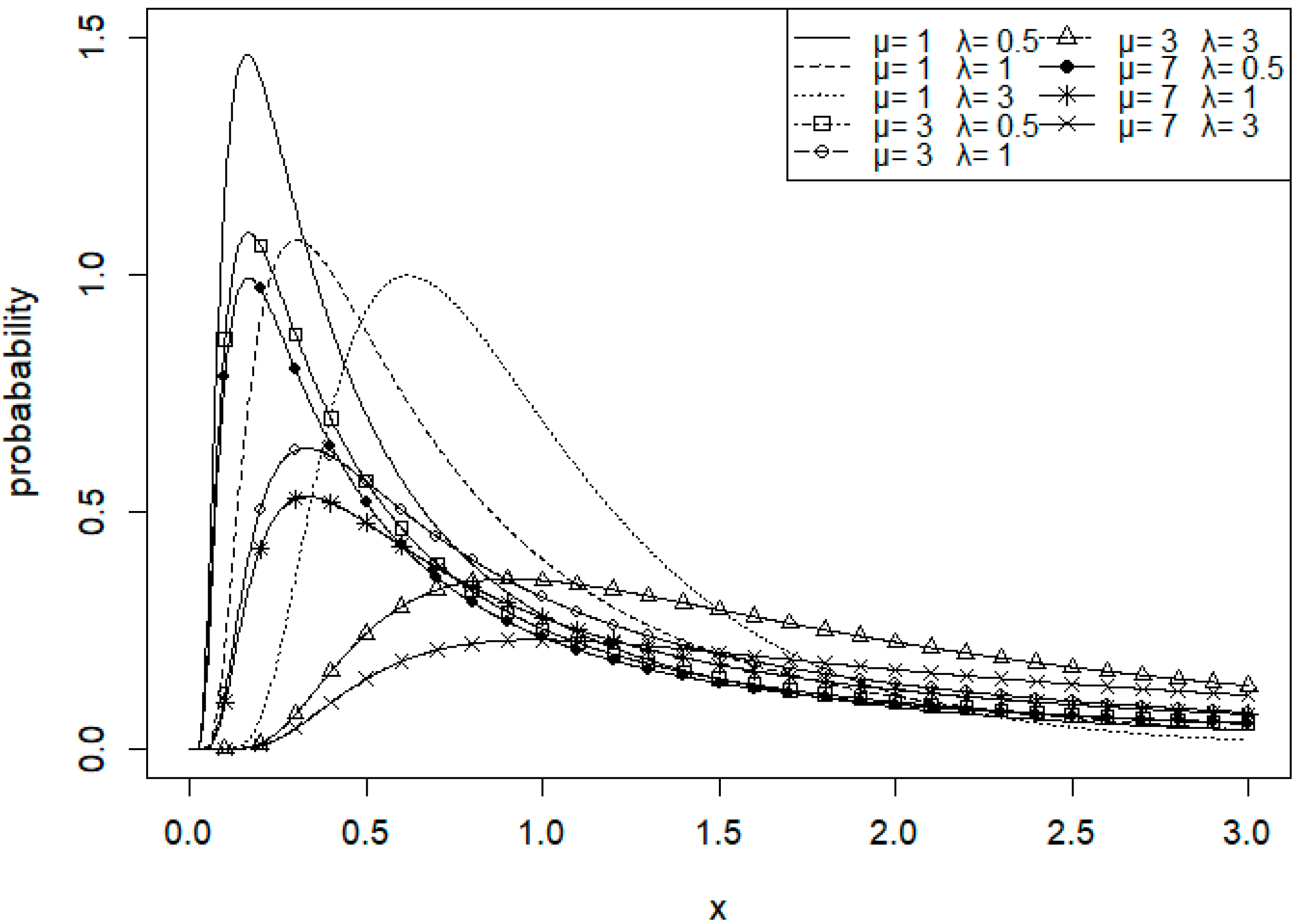
where $x>0,\hspace{0.33em}\mu >0,$ and $\lambda >0$. The shapes of the IG distributions with varying parameter sets are depicted in Figure 1. For lower values of $\lambda$ (0.5), the distribution demonstrates a higher peak and a steep decline in probability, which suggests a sharper distribution. As $\lambda$ increases, the peak becomes less pronounced, indicating a distribution with a heavier tail. Furthermore, an increase in $\mu$ causes a rightward shift in the distribution, representing higher mean values.

The mean of the IG distribution is μ, and the variance is ${\mu }^3/\lambda$ [3]. The maximum likelihood estimates (MLEs) of μ and λ are:

$${\widehat{\mu }}_{ML}=\overline{X}={\displaystyle \sum _{i=1}^n{X}_i}/n \mathrm{and} {\widehat{\lambda }}_{{}_{ML}}=n/{\displaystyle \sum _{i=1}^n\left(1/X_i-1/\overline{X}\right)},$$

(2)

where $X_1,\hspace{0.33em}\dots ,X_n$ are random samples from IG($\mu ,\lambda )$. Furthermore, it is also known that $\overline{X}~IG(\mu ,n\lambda )$, $\lambda {\displaystyle \sum _{i=1}^n\left(1/X_i-1/\overline{X}\right)}~{\chi }_{n-1}^2$, and $\overline{X}$ and $\lambda {\displaystyle \sum _{i=1}^n\left(1/X_i-1/\overline{X}\right)}$ are independent [16]. Folks and Chhikara [1] proved that the uniformly minimum variance unbiased estimators for μ and λ are:

$${\widehat{\mu }}_{UMVUE}=\overline{X}={\displaystyle \sum _{i=1}^n{X}_i}/n \mathrm{and} {\widehat{\lambda }}_{{}_{UMVUE}}=\left(n-3\right)/{\displaystyle \sum _{i=1}^n\left(1/X_i-1/\overline{X}\right)}.$$

The necessity of using confidence intervals (CIs) for estimating the mean of the IG distribution rather than relying solely on point estimators is pivotal in statistical analysis. Confidence intervals provide a range within which the true mean is likely to fall, reflecting the uncertainty inherent in using sample data to estimate population parameters. In contrast to a single point estimate, confidence intervals offer a more nuanced and informative picture, essential for rigorous statistical inference and decision-making in fields like survival analysis and reliability engineering, where precise estimation is key [17].

This paper focuses on Wald’s interval, a fundamental tool in statistical inference known for its simplicity and broad applicability. Wald’s interval is derived from the Wald test, which is based on the asymptotic normality of maximum likelihood estimators. It offers a direct method for constructing confidence intervals, particularly when the sample size is large [18]. However, the finite sample distributions of Wald tests are often not well defined [19]. Constructing Wald CIs for single-parameter models is straightforward, but when dealing with the IG distribution, which involves two parameters, the profile likelihood method is more advantageous. Non-normal distributions or small sample sizes may render Wald CIs unsuitable. To fix this, we can use reparameterization to create Wald CIs using the profile likelihood method. This makes sure that the sampling distribution is more like the normal distribution, which is a key assumption of the Wald method. Furthermore, using expected Fisher information in Wald CIs can offer more stability and be less sensitive to sample-specific irregularities.

In this study, CIs for the mean parameter of the IG distribution are constructed for scenarios where the shape parameter is unknown, focusing primarily on marginal intervals. We investigate two specific types of CIs: the first is the Wald-type CI using profile likelihood without reparameterization, and the second is the Wald-type CI incorporating reparameterization and utilizing expected Fisher information. These two proposed intervals are compared with existing intervals through simulation studies.

The rest of the paper is structured as follows: Section 2 presents intervals in literature. Section 3 presents the mathematical derivation of the Wald-type profile likelihood and Wald-type reparametrized profile likelihood with expected Fisher information intervals. Section 4 details the properties of these proposed intervals. Section 5 describes the simulation studies conducted to compare the performance of the proposed intervals with existing methods. Section 6 applies the proposed intervals to a real dataset. The paper concludes with a discussion in Section 7, where the findings are summarized and potential avenues for future research are outlined.

Table 1. List of abbreviations and acronyms used in the paper.

Abbreviations	Definitions
AIC	Akaike information criterion
AIL	Average interval length
CI	Confidence interval
CP	Coverage probability
IG	Inverse Gaussian
MLE	Maximum likelihood estimator
PL	Profile likelihood
RPL	Reparameterized profile likelihood
WPL	Wald-type profile likelihood (without reparameterization)
WRPLE	Wald-type reparameterized profile likelihood using expected Fisher information
WRPLO	Wald-type reparameterized profile likelihood using observed Fisher information

provides a list of detailed abbreviations and definitions used in this paper.

2. Intervals in Literature

2.1. Wald-Type Confidence Interval

The Wald confidence interval is typically constructed around a maximum likelihood estimator (MLE), leveraging the properties of a normal distribution, especially for large samples [20]. The calculation of this interval is based on the Wald test, which is used to evaluate the null hypothesis $H_0:\theta ={\theta }_0$ against an alternative $H_a:\theta ={\theta }_1$. Under $H_0$, two key statistics are used, both exhibiting asymptotic normal distributions as the sample size increases:

$$\sqrt{I\left({\hat{\theta }}_{ML}\right)}\left({\hat{\theta }}_{ML}-{\theta }_0\right)\hspace{0.33em}\stackrel{a}{~}\hspace{0.33em}N(0,1) \mathrm{and} \sqrt{J\left({\widehat{\theta }}_{ML}\right)}\left({\widehat{\theta }}_{ML}-{\theta }_0\right)\hspace{0.33em}\stackrel{a}{~}\hspace{0.33em}N(0,1),$$

(3)

where $I\left({\widehat{\theta }}_{ML}\right)$ and $J\left({\widehat{\theta }}_{ML}\right)$ represent the estimated observed and expected Fisher information, respectively [21]. The observed and expected Fisher information are defined as:

$$I\left(\theta \right)=-\frac{{\partial }^{2}L\left(\theta ;\underset{˜}{x}\right)}{\partial {\theta }^2} \mathrm{and} J\left(\theta \right)=-E\left[\frac{{\partial }^{2}L\left(\theta ;\underset{˜}{X}\right)}{\partial {\theta }^2}\right].$$

(4)

Construct the Wald confidence interval using the formula:

$${\widehat{\theta }}_{ML}\pm z_{\alpha /2}\sqrt{1/I\left({\widehat{\theta }}_{ML}\right)} \mathrm{or} {\widehat{\theta }}_{ML}\pm z_{\alpha /2}\sqrt{1/J\left({\widehat{\theta }}_{ML}\right)}.$$

(5)

It is worth noting that the Wald statistics can be written in

$$W=I\left({\widehat{\theta }}_{ML}\right)\left({\widehat{\theta }}_{ML}-\theta \right){\hspace{0.33em}}^2,$$

(6)

which is the quadratic approximation of $-2\log \Lambda (\theta )=-2\log \left(L\left(\theta ;\underset{˜}{x}\right)/L({\widehat{\theta }}_{ML};\underset{˜}{x})\right)$. The Wald statistic follows an asymptotic chi-squared distribution, with the degrees of freedom equal to the number of parameters being tested.

2.2. Profile-Likelihood-Based Confidence Interval

Statistical inference uses the profile likelihood confidence interval method to estimate confidence intervals for a parameter of interest in a model with multiple parameters. This approach is particularly useful in complex models where direct computation of the confidence interval for a parameter is challenging due to the presence of nuisance parameters—other parameters in the model that are not of primary interest [22,23]. In the profile likelihood method, the process involves:

• The likelihood function: Suppose we have a likelihood function $L(\theta ,\varphi )$, where $\theta$ is the parameter of interest and $\varphi$ represents nuisance parameters. The full likelihood is a function of both of these sets of parameters.
• Profiling out nuisance parameters: To focus on $\theta$, we maximize the likelihood function over the nuisance parameters $\varphi$for each fixed value of $\theta$. This gives us the profile likelihood function for $\theta$: $L_P(\theta )={\max }_{\varphi }L(\theta ,\varphi )$.
• Estimation of the parameter of interest: The estimate $\widehat{\theta }$ is obtained by maximizing the profile likelihood as follows:

$$\widehat{\theta }=\arg {\max }_{\theta }{L}_P(\theta );$$

4.

Constructing the confidence interval: The confidence interval for $\theta$ is then constructed based on the profile likelihood, so the interval is as follows:

$$\left\{\theta \left|-2\log \left(\frac{L_P(\theta )}{L_P(\widehat{\theta })}\right)\le {\chi }_{1-\alpha ,\mathrm{d}.\mathrm{f}.}^2\right.\right\},$$

(7)

where ${\chi }_{1-\alpha ,\mathrm{d}.\mathrm{f}.}^2$ is the critical value from the chi-squared distribution with degrees of freedom equal to the number of parameters being estimated (often 1 for a single parameter), and $\alpha$ is the significance level (e.g., 0.05 for a 95% confidence interval).

While likelihood-based and profile-likelihood-based intervals typically lack a closed form, which can be seen as a drawback compared to the more straightforward Wald-type interval with its closed-form solutions for many situations, this study focuses on applying the construction of a Wald-type interval to the profile likelihood. This approach aims to leverage the benefits of both methods, offering a more practical solution for statistical analysis.

2.3. Existing Confidence Intervals

For the IG distribution, as shown in (1), there are two parameters. In cases where the shape parameter is known, Arefi et al. [24] proposed CIs for the mean parameter, which are (1) the Wald CI: $\overline{X}\pm z_{1-\alpha /2}{\overline{X}}^{3/2}/\sqrt{n\lambda }$; (2) the score CI, derived from solving $-z_{1-\alpha /2}\le \sqrt{n\lambda }\left(\overline{X}-\mu \right)/\sqrt{{\mu }^3}\le z_{1-\alpha /2}$; and (3) the CI obtained from the likelihood ratio:

$$\frac{n\lambda \overline{X}}{n\lambda +k\sqrt{n\lambda \overline{X}}}\le \mu \le \frac{n\lambda \overline{X}}{n\lambda -k\sqrt{n\lambda \overline{X}}},$$

(8)

where $k=\sqrt{{\chi }_{1,(1-\alpha )}^2}$ and $0<k<\sqrt{n\lambda /\overline{X}}$. In a case where both parameters are unknown, Srisuradetchai [25] proposed the formula for the profile-likelihood-based (PL) CI as:

$$\frac{-n+\sqrt{n^2+Bn\overline{X}}}{B}\le \mu \le \frac{-n-\sqrt{n^2+Bn\overline{X}}}{B},$$

(9)

where $B=\left(\frac{\widehat{\mu }{\displaystyle \sum _{i=1}^n{X}_i^{-1}-n}}{\widehat{\mu }\exp \left(-{\chi }_{1,(1-\alpha )}^2/n\right)}\right)-{\displaystyle \sum _{i=1}^n{X}_i^{-1}}$. Díaz-Francés [26] derived the reparameterized profile likelihood (RPL) CI as:

$${\left(\widehat{\phi }+\frac{\sqrt{n(c^{-2/n}-1)}}{\sqrt{\widehat{\lambda }{\displaystyle {\sum }_{i=1}^n{X}_i}}}\right)}^{-1}\le \mu \le {\left(\widehat{\phi }-\frac{\sqrt{n(c^{-2/n}-1)}}{\sqrt{\widehat{\lambda }{\displaystyle {\sum }_{i=1}^n{X}_i}}}\right)}^{-1},$$

(10)

where $c=\exp \left(-{\chi }_{1-\alpha ,1}^2/n\right)$ and $\widehat{\phi }={\widehat{\mu }}^{-1}=n/{\displaystyle {\sum }_{i=1}^n{X}_i}$. Srisuradetchai [27] used reparameterized profile likelihoods to construct a Wald-type reparameterized profile likelihood using observed Fisher information (WRPLO) CI for the mean of the IG distribution. The interval is:

$${\left(\frac{n}{{\displaystyle {\sum }_{i=1}^n{X}_i}}+z_{1-\frac{\alpha }{2}}\sqrt{\frac{1}{\widehat{\lambda }{\displaystyle {\sum }_{i=1}^n{X}_i}}}\right)}^{-1}\le \mu \le {\left(\frac{n}{{\displaystyle {\sum }_{i=1}^n{X}_i}}-z_{1-\frac{\alpha }{2}}\sqrt{\frac{1}{\widehat{\lambda }{\displaystyle {\sum }_{i=1}^n{X}_i}}}\right)}^{-1},$$

(11)

where $\widehat{\lambda }={\left(\frac{{\displaystyle {\sum }_{i=1}^n{X}_i^{-1}}}{n}-\frac{1}{\overline{X}}\right)}^{-1}$.

In the literature, the Wald-type profile-likelihood-based (WPL) interval and the Wald-type reparameterized profile-likelihood interval with expected Fisher information (WRPLE) are not present. Using expected Fisher information generally leads to intervals that are more stable across different samples, while intervals based on observed Fisher information can be more sensitive to the specificities of the data set. Furthermore, these two types of CIs will be derived and compared to the PL, RPL, and WRPLO through Monte Carlo simulations.

3. Mathematical Results

This section will focus on the mathematical derivation of two statistical intervals: the WPL and the WRPLE.

3.1. Wald-Type Profile-Likelihood-Based Interval

The full log-likelihood function based on the observed random sample size of $n$, $x_{obs}=\left(x_1,x_2,\dots ,x_n\right),$ is as follows:

$$l(\mu ,\lambda )=\log L(\mu ,\lambda )=\frac{n}{2}\log \lambda -\frac{n}{2}\log (2\pi )-\frac{3}{2}{\displaystyle \sum _{i=1}^n\log x_i}-\frac{\lambda }{2}\left(\frac{{\displaystyle \sum _{i=1}^n{x}_i}}{{\mu }^2}+{\displaystyle \sum _{i=1}^n\frac{1}{x_i}}\right)+\frac{n\lambda }{\mu }.$$

To focus on $\mu$, we maximize the likelihood function over the nuisance parameters $\lambda$ for each fixed value of $\mu$ by solving $\frac{\partial }{\partial \lambda }l(\mu ,\lambda )\stackrel{set}{=}0$. Then,

$$\tilde{\lambda }={\left(\frac{{\displaystyle \sum _{i=1}^n{x}_i^{}}}{n{\mu }^2}+\frac{{\displaystyle \sum _{i=1}^n{x}_i^{-1}}}{n}-\frac{2}{\mu }\right)}^{-1}.$$

(12)

This gives us the log profile likelihood function for $\theta$:

$$l_P(\mu )=l(\mu ,\tilde{\lambda })=c-\frac{n}{2}+\frac{n}{2}\log (n\mu )-\frac{n}{2}\log \left(\mu {\displaystyle \sum _{i=1}^n{x}_i^{-1}+\frac{{\displaystyle \sum _{i=1}^n{x}_i^{}}}{\mu }}-2n\right).$$

The estimate $\widehat{\mu }$ is obtained by maximizing the profile likelihood $l_P(\mu )$. Consider

$$\begin{array}{l}{S}_p(\mu )=\frac{\partial l_p(\mu )}{\partial \mu }=\frac{\partial }{\partial \mu }\left(c-\frac{n}{2}+\frac{n}{2}\log (n\mu )-\frac{n}{2}\log \left(\mu {\displaystyle \sum _{i=1}^n{x}_i^{-1}+\frac{1}{\mu }}{\displaystyle \sum _{i=1}^n{x}_i^{}}-2n\right)\right)\\ \hspace{1em}\hspace{1em}=\frac{n}{2\mu }-\frac{n}{2}\frac{\left({\displaystyle \sum _{i=1}^n{x}_i^{-1}}-\frac{n\widehat{\mu }}{{\mu }^2}\right)}{\left(\mu {\displaystyle \sum _{i=1}^n{x}_i^{-1}+\frac{1}{\mu }}{\displaystyle \sum _{i=1}^n{x}_i^{}}-2n\right)}=\frac{n}{2\mu }-\frac{n}{2\mu }\frac{\left({\displaystyle \sum _{i=1}^n{x}_i^{-1}}-\frac{1}{{\mu }^2}{\displaystyle \sum _{i=1}^n{x}_i^{}}\right)}{\left({\displaystyle \sum _{i=1}^n{x}_i^{-1}}+\frac{1}{{\mu }^2}{\displaystyle \sum _{i=1}^n{x}_i^{}}-\frac{2n}{\mu }\right)}\\ \hspace{1em}\hspace{1em}=\frac{n}{2\mu }-\frac{n}{2\mu }{\left({\displaystyle \sum _{i=1}^n{x}_i^{-1}}+\frac{1}{{\mu }^2}{\displaystyle \sum _{i=1}^n{x}_i^{}}-\frac{2n}{\mu }\right)}^{-1}\left({\displaystyle \sum _{i=1}^n{x}_i^{-1}}-\frac{1}{{\mu }^2}{\displaystyle \sum _{i=1}^n{x}_i^{}}\right).\end{array}$$

Then, solving $S_p(\mu )\stackrel{set}{=}0$ will give $\widehat{\mu }={\displaystyle \sum _{i=1}^n{x}_i}/n$. Next, we will find the observed Fisher information:

$$I_p(\mu )=-\frac{\partial S_p(\mu )}{\partial \mu }=-\left(-\frac{n}{2{\mu }^2}-\left(\frac{3n}{2{\mu }^4}{\displaystyle \sum _{i=1}^n{x}_i^{}}-\frac{n{\displaystyle \sum _{i=1}^n{x}_i^{-1}}}{2{\mu }^2}\right){\left({\displaystyle \sum _{i=1}^n{x}_i^{-1}}+\frac{1}{{\mu }^2}{\displaystyle \sum _{i=1}^n{x}_i^{}}-\frac{2n}{\mu }\right)}^{-1}\right.$$

$$\left.-\left(\frac{n{\displaystyle \sum _{i=1}^n{x}_i^{-1}}}{2\mu }-\frac{n}{2{\mu }^3}{\displaystyle \sum _{i=1}^n{x}_i^{}}\right)\left(\frac{2n}{{\mu }^2}-\frac{2}{{\mu }^3}{\displaystyle \sum _{i=1}^n{x}_i^{}}\right){\left({\displaystyle \sum _{i=1}^n{x}_i^{-1}}+\frac{1}{{\mu }^2}{\displaystyle \sum _{i=1}^n{x}_i^{}}-\frac{2n}{\mu }\right)}^{-2}\right).$$

And the inverse of the Fisher information is $I_p^{-1}(\mu )=1/I_p(\mu )$. Term $I_p^{-1}(\mu )$ can be simplified as follows:

$$\begin{array}{l}{I}_p^{-1}(\widehat{\mu })=\\ \left[\frac{n}{2{\overline{x}}^2}+\left(\frac{3n^2}{2{\overline{x}}^3}-\frac{n{\displaystyle \sum _{i=1}^n{x}_i^{-1}}}{2{\overline{x}}^2}\right){\left({\displaystyle \sum _{i=1}^n{x}_i^{-1}}+\frac{n}{\overline{x}}-\frac{2n}{\overline{x}}\right)}^{-1}\right.+{\left.\left(\frac{n{\displaystyle \sum _{i=1}^n{x}_i^{-1}}}{2\overline{x}}-\frac{n^2}{2{\overline{x}}^2}\right)\left(\frac{2n}{{\overline{x}}^2}-\frac{2n}{{\overline{x}}^2}\right){\left({\displaystyle \sum _{i=1}^n{x}_i^{-1}}+\frac{n}{\overline{x}}-\frac{2n}{\overline{x}}\right)}^{-2}\right]}^{-1}\\ ={\left[\frac{n}{2{\overline{x}}^2}-\frac{n}{2{\overline{x}}^2}\left({\displaystyle \sum _{i=1}^n{x}_i^{-1}}-\frac{3n}{\overline{x}}\right){\left({\displaystyle \sum _{i=1}^n{x}_i^{-1}}-\frac{n}{\overline{x}}\right)}^{-1}\right]}^{-1}={\left[\frac{n}{2{\overline{x}}^2}\left[1-\frac{\left({\displaystyle \sum _{i=1}^n{x}_i^{-1}}-\frac{n}{\overline{x}}\right)}{\left({\displaystyle \sum _{i=1}^n{x}_i^{-1}}-\frac{n}{\overline{x}}\right)}+\frac{\frac{2n}{\overline{x}}}{\left({\displaystyle \sum _{i=1}^n{x}_i^{-1}}-\frac{n}{\overline{x}}\right)}\right]\right]}^{-1}\\ ={\left[\frac{n}{2{\overline{x}}^2}\frac{\frac{2n}{\overline{x}}}{\left({\displaystyle \sum _{i=1}^n{x}_i^{-1}}-\frac{n}{\overline{x}}\right)}\right]}^{-1}={\left[\frac{n^2}{{\overline{x}}^3}{\left({\displaystyle \sum _{i=1}^n{x}_i^{-1}}-\frac{n}{\overline{x}}\right)}^{-1}\right]}^{-1}=\frac{{\overline{x}}^3}{n\widehat{\lambda }}.\end{array}$$

(13)

Thus, the $(1-\alpha )\%$ WPL interval is

$$\overline{X}-z_{1-\frac{\alpha }{2}}\sqrt{\frac{{\overline{X}}^3}{n\widehat{\lambda }}}\le \hspace{1em}\mu \hspace{1em}\le \overline{X}+z_{1-\frac{\alpha }{2}}\sqrt{\frac{{\overline{X}}^3}{n\widehat{\lambda }}},$$

(14)

and when we substitute $\widehat{\lambda }=n/{\displaystyle {\sum }_{i=1}^n(1/X_i-1/\overline{X})}$, the corresponding WPL interval for $\mu$ will be

$$\overline{X}-z_{1-\frac{\alpha }{2}}\frac{\overline{X}}{n}\sqrt{\overline{X}{\displaystyle \sum _{i=1}^n\left(\frac{1}{X_i}-\frac{1}{\overline{X}}\right)}} \le \hspace{1em}\mu \hspace{1em}\le \overline{X}+z_{1-\frac{\alpha }{2}}\frac{\overline{X}}{n}\sqrt{\overline{X}{\displaystyle \sum _{i=1}^n\left(\frac{1}{X_i}-\frac{1}{\overline{X}}\right)}},$$

(15)

where $z_{1-\frac{\alpha }{2}}$ is the $(1-\alpha /2)$th quantile of the standard normal.

3.2. Wald-Type Reparameterized Profile Likelihood with Expected Fisher Information

The full log-likelihood function based on the observed random sample size of $n$, $x_{obs}=\left(x_1,x_2,\dots ,x_n\right),$ is as follows:

$$l(\mu ,\lambda )=\log L(\mu ,\lambda )=\frac{n}{2}\log \lambda -\frac{n}{2}\log (2\pi )-\frac{3}{2}{\displaystyle \sum _{i=1}^n\log x_i}-\frac{\lambda }{2}\left(\frac{{\displaystyle \sum _{i=1}^n{x}_i}}{{\mu }^2}+{\displaystyle \sum _{i=1}^n\frac{1}{x_i}}\right)+\frac{n\lambda }{\mu }$$

Using reparameterization $\mu ={\phi }^{-1}$, the full log-likelihood function becomes

$$l(\phi ,\lambda )=\frac{n}{2}\log (\lambda )-\frac{n}{2}\log (2\pi )-\frac{3}{2}{\displaystyle \sum _{i=1}^n\log x_i}-\frac{\lambda {\phi }^2{\displaystyle {\sum }_{i=1}^n{x}_i}}{2}-\frac{\lambda }{2}{\displaystyle {\sum }_{i=1}^n{x}_i^{-1}}+n\lambda \phi .$$

To focus on $\phi$, we maximize $l(\phi ,\lambda )$ over the nuisance parameters $\lambda$ for each fixed value of $\mu$ by solving $\frac{\partial }{\partial \lambda }l(\phi ,\lambda )\stackrel{set}{=}0$. Then,

$$\tilde{\lambda }(\phi )=n{\left({\phi }^2{\displaystyle \sum _{i=1}^n{x}_i}-2n\phi +{\displaystyle \sum _{i=1}^n{x}_i^{-1}}\right)}^{-1},$$

(16)

By plugging in $\tilde{\lambda }(\phi )$ into $l(\phi ,\lambda )$, we obtain the log reparameterized profile likelihood function as follows:

$$\begin{array}{ll}{l}_p(\phi ,\tilde{\lambda }(\phi ))& =\frac{n}{2}\log (\tilde{\lambda }(\phi ))-\frac{\tilde{\lambda }(\phi ){\phi }^2{\displaystyle {\sum }_{i=1}^n{x}_i}}{2}-\frac{\tilde{\lambda }(\phi )}{2}{\displaystyle {\sum }_{i=1}^n{x}_i^{-1}}+n\tilde{\lambda }(\phi )\phi +c\\ & =\frac{n}{2}\log (\tilde{\lambda }(\phi ))-\frac{\tilde{\lambda }(\phi )}{2}\left({\phi }^2{\displaystyle {\sum }_{i=1}^n{x}_i}-2n\phi +{\displaystyle {\sum }_{i=1}^n{x}_i^{-1}}\right)+c\\ & =\frac{n}{2}\log (n)-\frac{n}{2}\log ({\phi }^2{\displaystyle \sum _{i=1}^n{x}_i}-2n\phi +{\displaystyle \sum _{i=1}^n{x}_i^{-1}})-\frac{n}{2}+c,\end{array}$$

where $c=-\frac{n}{2}\log (2\pi )-\frac{3}{2}{\displaystyle \sum _{i=1}^n\log x_i}$. The score function of log reparametrized profile likelihood is as follows:

$$\begin{array}{ll}{S}_p(\phi )& =\frac{\partial l_p(\phi ,\tilde{\lambda }(\phi ))}{\partial \phi }=-\frac{n}{2}{\left({\phi }^2{\displaystyle \sum _{i=1}^n{x}_i}-2n\phi +{\displaystyle \sum _{i=1}^n{x}_i^{-1}}\right)}^{-1}\left(2\phi {\displaystyle \sum _{i=1}^n{x}_i}-2n\right)\\ & =-n\left(\phi {\displaystyle \sum _{i=1}^n{x}_i}-n\right){\left({\phi }^2{\displaystyle \sum _{i=1}^n{x}_i}-2n\phi +{\displaystyle \sum _{i=1}^n{x}_i^{-1}}\right)}^{-1}.\end{array}$$

The observed Fisher information is the negative of the second derivative of log reparameterized profile likelihood, as follows:

$$\begin{array}{l}{I}_p(\phi )=-\frac{\partial S_p(\phi )}{\partial \phi }\\ =-\left(\frac{(n\phi {\displaystyle \sum _{i=1}^n{x}_i}-n^2)(2\phi {\displaystyle \sum _{i=1}^n{x}_i}-2n)}{{\left({\phi }^2{\displaystyle \sum _{i=1}^n{x}_i}-2n\phi +{\displaystyle \sum _{i=1}^n{x}_i^{-1}}\right)}^2}-\frac{n{\displaystyle \sum _{i=1}^n{x}_i}}{\left({\phi }^2{\displaystyle \sum _{i=1}^n{x}_i}-2n\phi +{\displaystyle \sum _{i=1}^n{x}_i^{-1}}\right)}\right)\\ =\frac{n{\displaystyle \sum _{i=1}^n{x}_i}}{\left({\phi }^2{\displaystyle \sum _{i=1}^n{x}_i}-2n\phi +{\displaystyle \sum _{i=1}^n{x}_i^{-1}}\right)}-\frac{(n\phi {\displaystyle \sum _{i=1}^n{x}_i}-n^2)(2\phi {\displaystyle \sum _{i=1}^n{x}_i}-2n)}{{\left({\phi }^2{\displaystyle \sum _{i=1}^n{x}_i}-2n\phi +{\displaystyle \sum _{i=1}^n{x}_i^{-1}}\right)}^2}\\ =\frac{-n{\phi }^2{\left({\displaystyle \sum _{i=1}^n{x}_i}\right)}^2+n{\displaystyle \sum _{i=1}^n{x}_i}{\displaystyle \sum _{i=1}^n{x}_i^{-1}}+2n^2\phi {\displaystyle \sum _{i=1}^n{x}_i}-2n^3}{{\left({\phi }^2{\displaystyle \sum _{i=1}^n{x}_i}-2n\phi +{\displaystyle \sum _{i=1}^n{x}_i^{-1}}\right)}^2}.\end{array}$$

The expectation of the observed Fisher information can be calculated as follows:

$$J_p(\phi )=E\left[I_p(\phi )\right]=E\left[\frac{-n{\phi }^2{\left({\displaystyle \sum _{i=1}^n{X}_i}\right)}^2+n{\displaystyle \sum _{i=1}^n{X}_i}{\displaystyle \sum _{i=1}^n{X}_i^{-1}}+2n^2\phi {\displaystyle \sum _{i=1}^n{X}_i}-2n^3}{{\left({\phi }^2{\displaystyle \sum _{i=1}^n{X}_i}-2n\phi +{\displaystyle \sum _{i=1}^n{X}_i^{-1}}\right)}^2}\right]$$

(17)

Using a first-order Taylor approximation for a function of two variables, the expectation becomes:

$$J_p(\phi )\approx \frac{E\left[-n{\phi }^2{\left({\displaystyle \sum _{i=1}^n{X}_i}\right)}^2+n{\displaystyle \sum _{i=1}^n{X}_i}{\displaystyle \sum _{i=1}^n{X}_i^{-1}}+2n^2\phi {\displaystyle \sum _{i=1}^n{X}_i}-2n^3\right]}{E\left[{\left({\phi }^2{\displaystyle \sum _{i=1}^n{X}_i}-2n\phi +{\displaystyle \sum _{i=1}^n{X}_i^{-1}}\right)}^2\right]}.$$

(18)

Since $E\left(X\right)=\mu$, $Var\left(X\right)={\mu }^3/\lambda$, $E\left(1/X\right)=1/\mu +1/\lambda ,$$Var\left(1/X\right)=1/\left(\mu \lambda \right)+$$2/{\lambda }^2,$ and $E\left[{\displaystyle \sum _{i=1}^n{X}_i}{\displaystyle \sum _{i=1}^n{X}_i^{-1}}\right]=n^2+n^2\mu /\lambda -n\mu /\lambda$, term

$$\begin{array}{l}E\left[-n{\phi }^2{\left({\displaystyle \sum _{i=1}^n{X}_i}\right)}^2+n{\displaystyle \sum _{i=1}^n{X}_i}{\displaystyle \sum _{i=1}^n{X}_i^{-1}}+2n^2\phi {\displaystyle \sum _{i=1}^n{X}_i}-2n^3\right]\\ \hspace{1em}\hspace{1em}=-n{\phi }^{2}E\left[{\left({\displaystyle \sum _{i=1}^n{X}_i}\right)}^2\right]+nE\left[{\displaystyle \sum _{i=1}^n{X}_i}{\displaystyle \sum _{i=1}^n{X}_i^{-1}}\right]+2n^2\phi E\left[{\displaystyle \sum _{i=1}^n{X}_i}\right]+E\left[-2n^3\right]\\ \hspace{1em}\hspace{1em}=-n{\phi }^2\left(\frac{n{\mu }^3}{\lambda }+n^2{\mu }^2\right)+n\left(n^2+\frac{n^2\mu }{\lambda }-\frac{n\mu }{\lambda }\right)+2n^2\phi \left(n\mu \right)-2n^3\\ \hspace{1em}\hspace{1em}=-\frac{n^2{\phi }^2{\mu }^3}{\lambda }-n^3{\phi }^2{\mu }^2+n^3+\frac{n^3\mu }{\lambda }-\frac{n^2\mu }{\lambda }+2n^3\phi \mu -2n^3\\ \hspace{1em}\hspace{1em}=-\frac{n^2{\phi }^2}{{\phi }^3\lambda }-\frac{n^3{\phi }^2}{{\phi }^2}+n^3+\frac{n^3}{\phi \lambda }-\frac{n^2}{\phi \lambda }+\frac{2n^3\phi }{\phi }-2n^3=\frac{n^3}{\phi \lambda }-\frac{2n^2}{\phi \lambda }=\frac{n}{\lambda }\left(\frac{n(n-2)}{\phi }\right).\end{array}$$

The denominator of (18) can also be expressed as:

$$\begin{array}{l}E\left[{\left({\phi }^2{\displaystyle \sum _{i=1}^n{X}_i}-2n\phi +{\displaystyle \sum _{i=1}^n{X}_i^{-1}}\right)}^2\right]\\ \hspace{1em}=E\left[{\phi }^4{\left({\displaystyle \sum _{i=1}^n{X}_i}\right)}^2-4n{\phi }^3{\displaystyle \sum _{i=1}^n{X}_i}+2{\phi }^2{\displaystyle \sum _{i=1}^n{X}_i}{\displaystyle \sum _{i=1}^n{X}_i^{-1}}+4n^2{\phi }^2-4n\phi {\displaystyle \sum _{i=1}^n{X}_i^{-1}}+{\left({\displaystyle \sum _{i=1}^n{X}_i^{-1}}\right)}^2\right].\end{array}$$

(19)

Because

$$E\left[{\displaystyle \sum _{i=1}^n{X}_i^{-1}}\right]=\frac{n}{\mu }+\frac{n}{\lambda } \mathrm{and} E\left[{\left({\displaystyle \sum _{i=1}^n{X}_i^{-1}}\right)}^2\right]=\frac{n}{\mu \lambda }+\frac{2n}{{\lambda }^2}+\frac{n^2}{{\mu }^2}+\frac{2n^2}{\mu \lambda }+\frac{n^2}{{\lambda }^2},$$

(19) will become:

$$\begin{array}{l}E\left[{\left({\phi }^2{\displaystyle \sum _{i=1}^n{x}_i}-2n\phi +{\displaystyle \sum _{i=1}^n{x}_i^{-1}}\right)}^2\right]={\phi }^4\left(\frac{n{\mu }^3}{\lambda }+n^2{\mu }^2\right)-4n{\phi }^3\left(n\mu \right)+2{\phi }^2\left(n^2+\frac{n^2\mu }{\lambda }-\frac{n\mu }{\lambda }\right)\\ \hfill +4n^2{\phi }^2-4n\phi \left(\frac{n}{\mu }+\frac{n}{\lambda }\right)+\left(\frac{n}{\mu \lambda }+\frac{2n}{{\lambda }^2}+\frac{n^2}{{\mu }^2}+\frac{2n^2}{\mu \lambda }+\frac{n^2}{{\lambda }^2}\right).\end{array}$$

With $\mu ={\phi }^{-1}$,

$$\begin{array}{l}E\left[{\left({\phi }^2{\displaystyle \sum _{i=1}^n{X}_i}-2n\phi +{\displaystyle \sum _{i=1}^n{X}_i^{-1}}\right)}^2\right]\\ ={\phi }^4\left(\frac{n}{\lambda {\phi }^3}+\frac{n^2}{{\phi }^2}\right)-4n{\phi }^3\left(\frac{n}{\phi }\right)+2{\phi }^2\left(n^2+\frac{n^2}{\phi \lambda }-\frac{n}{\phi \lambda }\right)\\ \hfill +4n^2{\phi }^2-4n\phi \left(n\phi +\frac{n}{\lambda }\right)+\left(\frac{n\phi }{\lambda }+\frac{2n}{{\lambda }^2}+n^2{\phi }^2+\frac{2n^2\phi }{\lambda }+\frac{n^2}{{\lambda }^2}\right)=\frac{n}{\lambda }\left(\frac{n+2}{\lambda }\right)\end{array}$$

The expected Fisher information is calculated as follows:

$$J_p(\phi )=\frac{(n-2)}{(n+2)}\frac{n\lambda }{\phi },$$

(20)

and the corresponding standard error of the estimator $\phi$ is as follows:

$$\mathrm{s}.\mathrm{e}.(\widehat{\phi })=\sqrt{J_p^{-1}(\widehat{\phi })}=\sqrt{\frac{(n+2)}{(n-2)}\frac{\widehat{\phi }}{n\widehat{\lambda }}}=\sqrt{\frac{(n+2)}{(n-2)}\left(\frac{{\displaystyle {\sum }_{i=1}^n(1/X_i-1/\overline{X})}}{n^2\overline{X}}\right)}.$$

(21)

The WRPLE interval of $\phi$ will be

$$\frac{1}{\overline{X}}-z_{1-\frac{\alpha }{2}}\frac{1}{n}\sqrt{\frac{(n+2)}{(n-2)\overline{X}}{\displaystyle \sum _{i=1}^n\left(\frac{1}{X_i}-\frac{1}{\overline{X}}\right)}} \le \hspace{1em}\phi \hspace{1em}\le \hspace{0.33em}\hspace{0.33em}\frac{1}{\overline{X}}+z_{1-\frac{\alpha }{2}}\frac{1}{n}\sqrt{\frac{(n+2)}{(n-2)\overline{X}}{\displaystyle \sum _{i=1}^n\left(\frac{1}{X_i}-\frac{1}{\overline{X}}\right)}},$$

(22)

where $z_{1-\frac{\alpha }{2}}$ is the $(1-\alpha /2)$th quantile of the standard normal. Therefore, the WRPLE interval of $\mu$ is as follows:

$${\left[\frac{1}{\overline{X}}+z_{1-\frac{\alpha }{2}}\frac{1}{n}\sqrt{\frac{(n+2)}{(n-2)\overline{X}}{\displaystyle \sum _{i=1}^n\left(\frac{1}{X_i}-\frac{1}{\overline{X}}\right)}} \right]}^{-1}\le \hspace{1em}\mu \hspace{1em}\le \hspace{0.33em}\hspace{0.33em}{\left[\frac{1}{\overline{X}}-z_{1-\frac{\alpha }{2}}\frac{1}{n}\sqrt{\frac{(n+2)}{(n-2)\overline{X}}{\displaystyle \sum _{i=1}^n\left(\frac{1}{X_i}-\frac{1}{\overline{X}}\right)}}\right]}^{-1}.$$

(23)

4. Some Properties of the Proposed Intervals

Because the Wald statistics in (6) is the quadratic approximation of $-2\log \Lambda (\theta )$ and from (7), some conditions are required for constructing a confidence interval.

4.1. A Condition for the WPL Interval

Let $X_1,X_2,\dots ,X_n$ be a random sample of size n from a population with an inverse Gaussian distribution with unknown mean parameter $\mu$ and shape parameter $\lambda .$ Because the Wald statistics is a quadratic approximation of $-2\log \Lambda (\mu )=$$-2\log \left(L_P\left(\mu ;\underset{˜}{x}\right)/L_P(\widehat{\mu };\underset{˜}{x})\right)$, and $-2\log \Lambda (\mu )$ has asymptotically chi-squared distribution, the lower and upper bounds of the WPL interval can be obtained if

$$\underset{\mu \to 0^{+}}{\lim }\hspace{0.33em}\hspace{0.33em}{I}_p(\widehat{\mu }){(\mu -\widehat{\mu })}^2\hspace{0.33em}\ge \hspace{0.33em}\hspace{0.33em}{\chi }_{1-\alpha ,1}^2 \mathrm{and} \underset{\mu \to \infty }{\lim }\hspace{0.33em}\hspace{0.33em}{I}_p(\widehat{\mu }){(\mu -\widehat{\mu })}^2\hspace{0.33em}\ge \hspace{0.33em}\hspace{0.33em}{\chi }_{1-\alpha ,1}^2,$$

respectively. Because $\underset{\mu \to 0^{+}}{\lim }\hspace{0.33em}\hspace{0.33em}{I}_p(\widehat{\mu }){(\mu -\widehat{\mu })}^2\hspace{0.33em}=I_p(\widehat{\mu }){\widehat{\mu }}^2$, and from (14) $I_p(\widehat{\mu })=n\widehat{\lambda }/{\widehat{\mu }}^3,$$\underset{\mu \to 0^{+}}{\lim }\hspace{0.33em}\hspace{0.33em}{I}_p(\widehat{\mu }){(\mu -\widehat{\mu })}^2\hspace{0.33em}=$$n\widehat{\lambda }/\widehat{\mu }.$ By substituting $\widehat{\mu }=\overline{X}$ and $\widehat{\lambda }=n/{\displaystyle {\sum }_{i=1}^n(1/X_i-1/\overline{X})}$, the condition for the lower bound of the WPL interval is as follows:

$$\frac{n^2}{\overline{X}}{\displaystyle \sum _{i=1}^n\left(\frac{1}{X_i}-\frac{1}{\overline{X}}\right)}\ge \hspace{0.33em}\hspace{0.33em}{\chi }_{1-\alpha ,1}^2.$$

And $\underset{\mu \to \infty }{\lim }\hspace{0.33em}\hspace{0.33em}{I}_p(\widehat{\mu }){(\mu -\widehat{\mu })}^2=\infty$, which is always greater than ${\chi }_{1-\alpha ,1}^2$. This means that an upper bound for the WPL interval does always exist, but a lower bound does depend on the data.

4.2. A Condition for the WRPLE Interval

Like the conditions of the WPL interval, the WRPLE interval can be found if and only if

$$\underset{\phi \to 0^{+}}{\lim }\hspace{0.33em}\hspace{0.33em}{J}_p(\widehat{\phi }){(\phi -\widehat{\phi })}^2\hspace{0.33em}\ge \hspace{0.33em}\hspace{0.33em}{\chi }_{1-\alpha ,1}^2 \mathrm{and} \underset{\widehat{\phi }\to \infty }{\lim }\hspace{0.33em}\hspace{0.33em}{J}_p(\widehat{\phi }){(\phi -\widehat{\phi })}^2\hspace{0.33em}\ge \hspace{0.33em}\hspace{0.33em}{\chi }_{1-\alpha ,1}^2.$$

(24)

Because $\underset{\phi \to 0^{+}}{\lim }\hspace{0.33em}\hspace{0.33em}{J}_p(\widehat{\phi }){(\phi -\widehat{\phi })}^2=J_p(\widehat{\phi }){\widehat{\phi }}^2$ and from (18), the condition for the lower bound of the WPL interval is

$$\frac{n^2}{\overline{X}}\frac{(n-2)}{(n+2)}{\left({\displaystyle {\sum }_{i=1}^n(1/X_i-1/\overline{X})}\right)}^{-1}\ge \hspace{0.33em}\hspace{0.33em}{\chi }_{1-\alpha ,1}^2.$$

(25)

For the upper bound, $\underset{\widehat{\phi }\to \infty }{\lim }\hspace{0.33em}\hspace{0.33em}{J}_p(\widehat{\phi }){(\phi -\widehat{\phi })}^2\hspace{0.33em}=\infty$, so the upper bound does always exist.

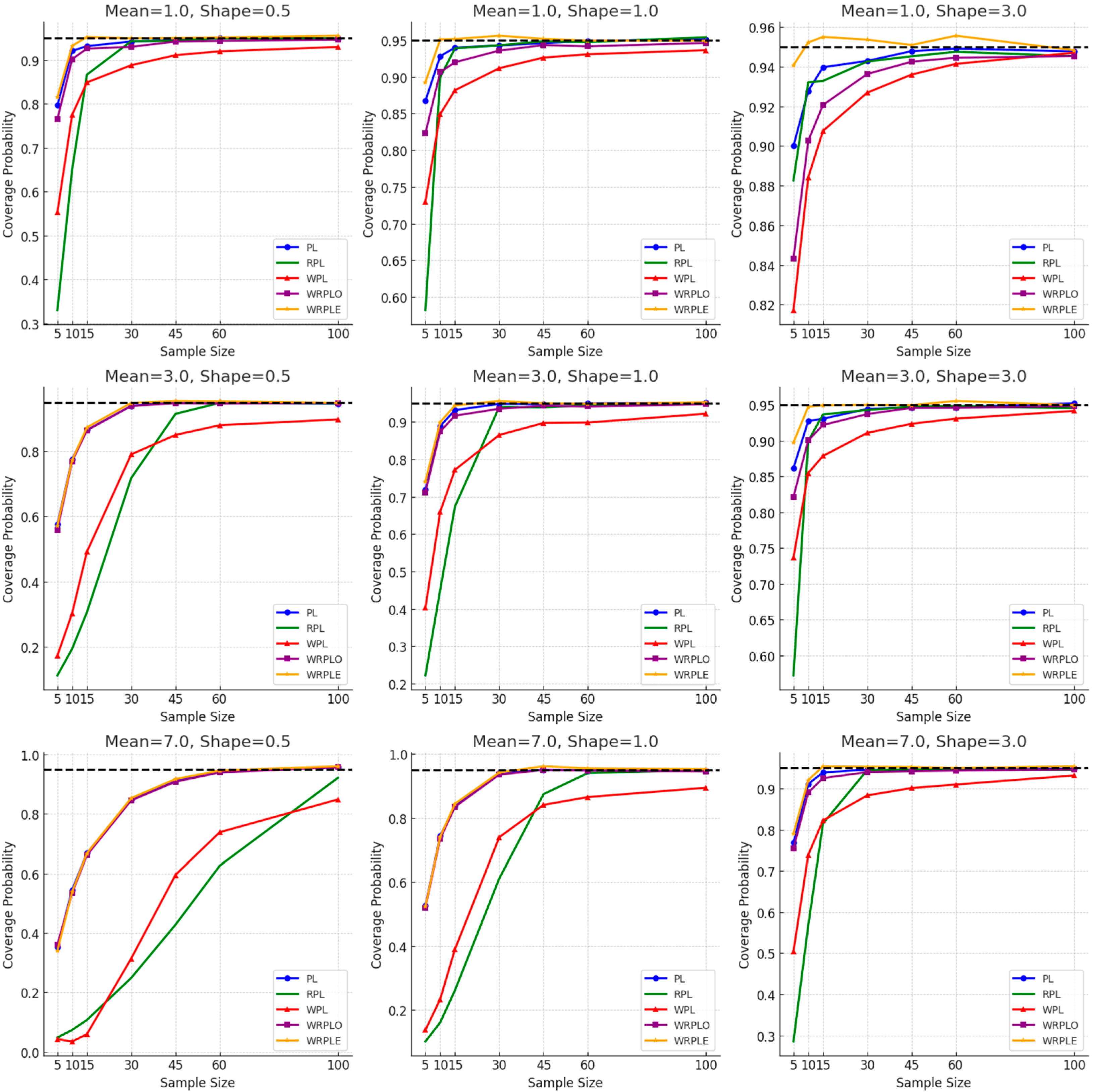
5. Simulation Studies

In the simulation studies, the sample sizes vary, including 5, 10, 15, 30, 45, 60, and 100. The mean parameter values are set at 1, 3, and 7, while the shape parameter values are 0.5, 1, and 3. The performance of two proposed distributions will be compared with the PL interval proposed by Srisuradetchai [25], the RPL approach by Díaz-Francés [26], and the WRPLO interval by Srisuradetchai [27]. Performance is evaluated in terms of coverage probability (CP) and average interval length (AIL). Results for the PL, RPL, and WRPLO are summarized in

Table 2. CPs and AILs of the PL interval proposed by Srisuradetchai [25].

$\mathit{\lambda }$ (Shape)	n	Coverage Probability			Average Interval Length
		$\mathit{\mu }$ (Mean)			$\mathit{\mu }$ (Mean)
		1	3	7	1	3	7
0.5	5	0.7964	0.5760	0.3520	22.5367	24.4815	33.5161
	10	0.9208	0.7760	0.5451	22.2293	43.1449	122.6111
	15	0.9315	0.8651	0.6673	8.1085	101.0214	79.8984
	30	0.9421	0.9393	0.8488	1.5772	48.3700	238.8934
	45	0.9453	0.9506	0.9129	1.0463	25.0285	151.0399
	60	0.9506	0.9499	0.9435	0.8505	8.8848	170.8275
	100	0.9486	0.9458	0.9566	0.6091	4.0184	93.0158
1	5	0.8673	0.7191	0.5269	33.0340	36.8387	50.0072
	10	0.9282	0.8887	0.7439	5.0073	49.1924	96.2266
	15	0.9398	0.9314	0.8373	1.7234	131.7031	125.8797
	30	0.9428	0.9479	0.9407	0.8561	12.5698	210.7568
	45	0.9459	0.9470	0.9507	0.6504	4.5521	112.0056
	60	0.9491	0.9495	0.9490	0.5468	3.4503	29.6077
	100	0.9510	0.9513	0.9487	0.4101	2.3437	10.9928
3	5	0.9000	0.8619	0.7681	2.9671	31.4322	94.2752
	10	0.9278	0.9276	0.9107	0.8994	14.7727	125.6737
	15	0.9397	0.9309	0.9388	0.6658	5.2189	68.1577
	30	0.9429	0.9445	0.9457	0.4372	2.5664	13.3481
	45	0.9478	0.9468	0.9453	0.3516	1.9552	8.3623
	60	0.9491	0.9468	0.9461	0.3011	1.6459	6.6398
	100	0.9477	0.9525	0.9477	0.2304	1.2300	4.6786

,

Table 3. CPs and AILs of the RPL approach proposed by Díaz-Francés [26].

$\mathit{\lambda }$ (Shape)	n	Coverage Probability			Average Interval Length
		$\mathit{\mu }$ (Mean)			$\mathit{\mu }$ (Mean)
		1	3	7	1	3	7
0.5	5	0.3295	0.1119	0.0472	6.4585	5.4885	5.3135
	10	0.6504	0.1939	0.073	1.0830	11.8711	33.6625
	15	0.8665	0.3058	0.1064	2.8495	3.7286	15.1804
	30	0.9427	0.7177	0.2481	1.5366	7.3637	55.9877
	45	0.9439	0.9147	0.4273	1.0440	4.2846	57.7240
	60	0.9494	0.9485	0.6258	0.8431	7.1018	23.9830
	100	0.9489	0.9470	0.9209	0.6089	3.9953	102.7412
1	5	0.5821	0.2221	0.101	2.9889	5.2536	6.6847
	10	0.8994	0.4506	0.1606	2.5446	4.5644	31.1419
	15	0.9390	0.6735	0.2613	1.6503	7.4503	6.2086
	30	0.9430	0.9399	0.6112	0.8524	7.2613	59.9609
	45	0.9484	0.9389	0.8747	0.6516	4.5042	26.5516
	60	0.9474	0.9446	0.9407	0.5494	3.4511	33.0396
	100	0.9539	0.9483	0.9502	0.4103	2.3522	10.9170
3	5	0.8826	0.5718	0.2852	0.4542	11.3641	23.5666
	10	0.9321	0.8996	0.5670	0.8896	2.2913	10.6808
	15	0.9328	0.9368	0.8145	0.6661	5.1338	35.5910
	30	0.9426	0.9431	0.9448	0.4393	2.5513	13.2340
	45	0.9452	0.9476	0.9464	0.3519	1.9498	8.3212
	60	0.9475	0.9484	0.9452	0.3004	1.6465	6.6264
	100	0.9453	0.9456	0.9455	0.2303	1.2319	4.6810

and

Table 4. CPs and AILs of the WRPLO proposed by Srisuradetchai [27].

$\mathit{\lambda }$ (Shape)	n	Coverage Probability			Average Interval Length
		$\mathit{\mu }$ (Mean)			$\mathit{\mu }$ (Mean)
		1	3	7	1	3	7
0.5	5	0.7648	0.5589	0.3605	27.1944	28.6415	33.6888
	10	0.9019	0.7685	0.5335	13.7167	47.1982	64.8575
	15	0.9258	0.8642	0.6606	41.7971	69.0019	77.2883
	30	0.9299	0.9391	0.8450	1.4503	60.1097	109.0317
	45	0.9419	0.9473	0.9078	1.0094	20.2874	236.1456
	60	0.9436	0.9463	0.9392	0.8315	7.8830	210.4629
	100	0.9460	0.9484	0.9565	0.6034	3.9255	54.9630
1	5	0.8231	0.7120	0.5208	14.1464	42.5124	66.7006
	10	0.9064	0.8742	0.7348	3.3469	51.0088	137.9784
	15	0.9199	0.9165	0.8348	1.4419	56.3881	139.6932
	30	0.9358	0.9349	0.9357	0.8242	8.5811	112.2808
	45	0.9433	0.9429	0.9505	0.6347	4.3697	101.5731
	60	0.9416	0.9409	0.9480	0.5385	3.3564	34.0264
	100	0.9462	0.9470	0.9461	0.4058	2.3274	10.7083
3	5	0.8433	0.8216	0.7539	2.2341	79.7818	63.8266
	10	0.9026	0.9005	0.8899	0.7785	12.3920	115.2107
	15	0.9207	0.9221	0.9250	0.6161	4.3373	69.4735
	30	0.9363	0.9374	0.9397	0.4228	2.4487	11.9999
	45	0.9425	0.9460	0.9418	0.3426	1.9033	8.0710
	60	0.9445	0.9461	0.9432	0.2960	1.6115	6.4183
	100	0.9453	0.9485	0.9465	0.2280	1.2217	4.6426

, and those for the proposed intervals are in

Table 5. CPs and AILs of the WPL interval.

$\mathit{\lambda }$ (Shape)	n	Coverage Probability			Average Interval Length
		$\mathit{\mu }$ (Mean)			$\mathit{\mu }$ (Mean)
		1	3	7	1	3	7
0.5	5	0.5525	0.1726	0.0420	1.0580	1.7659	2.0279
	10	0.7749	0.3031	0.0339	1.2895	2.3467	2.6358
	15	0.8488	0.4913	0.0586	1.3239	2.9065	3.3715
	30	0.8880	0.7904	0.3135	1.0114	4.0526	5.5555
	45	0.9109	0.8500	0.5950	0.8222	4.1752	7.3170
	60	0.9197	0.8799	0.7379	0.7182	3.8010	8.7419
	100	0.9296	0.8976	0.8482	0.5554	2.9112	9.9903
1	5	0.7302	0.4029	0.1370	1.1727	3.6745	3.6544
	10	0.8492	0.6596	0.2333	1.1591	3.4925	4.8826
	15	0.8818	0.7718	0.3898	0.9894	3.9176	6.0905
	30	0.9118	0.8648	0.7396	0.7104	3.7168	8.8713
	45	0.9263	0.8970	0.8410	0.5785	3.0658	9.9320
	60	0.9308	0.8981	0.8655	0.5030	2.6446	9.4724
	100	0.9364	0.9217	0.8947	0.3900	2.0447	7.3870
3	5	0.8172	0.7364	0.5044	0.8597	3.5417	7.0483
	10	0.8842	0.8549	0.7385	0.6686	3.4748	8.8143
	15	0.9076	0.8788	0.8220	0.5607	2.9499	9.4084
	30	0.9269	0.9111	0.8830	0.4044	2.1150	7.6076
	45	0.9360	0.9238	0.9009	0.3327	1.7348	6.2790
	60	0.9414	0.9310	0.9094	0.2896	1.5055	5.3961
	100	0.9470	0.9418	0.9315	0.2250	1.1740	4.2096

and

Table 6. CPs and AILs of the WRPLE interval.

$\mathit{\lambda }$ (Shape)	n	Coverage Probability			Average Interval Length
		$\mathit{\mu }$ (Mean)			$\mathit{\mu }$ (Mean)
		1	3	7	1	3	7
0.5	5	0.8153	0.5725	0.3391	31.7213	30.5061	23.4398
	10	0.9322	0.7728	0.5380	18.5406	44.8999	54.5505
	15	0.9523	0.8732	0.6671	23.4037	284.2358	89.1180
	30	0.9494	0.9482	0.8528	1.6982	81.8574	176.3652
	45	0.9500	0.9543	0.9168	1.0811	25.1390	122.5613
	60	0.9513	0.9533	0.9457	0.8660	10.1873	131.8133
	100	0.9553	0.9485	0.9599	0.6175	4.0827	74.6419
1	5	0.8928	0.7409	0.5241	16.0907	44.3857	66.7506
	10	0.9511	0.8992	0.7410	16.4258	111.8300	89.6045
	15	0.9516	0.9437	0.8447	2.1310	125.7302	125.1637
	30	0.9561	0.9558	0.9424	0.8933	11.1814	145.2397
	45	0.9518	0.9495	0.9619	0.6745	4.7340	124.8338
	60	0.9494	0.9482	0.9552	0.5590	3.5254	39.7383
	100	0.9493	0.9522	0.9529	0.4150	2.3912	11.1029
3	5	0.9407	0.8976	0.7898	6.5136	56.5863	120.0086
	10	0.9522	0.9476	0.9201	1.0494	21.7278	187.6656
	15	0.9550	0.9498	0.9536	0.7255	6.1024	165.2150
	30	0.9536	0.9503	0.9526	0.4533	2.6947	15.6644
	45	0.9509	0.9499	0.9521	0.3588	2.0194	8.5897
	60	0.9556	0.9557	0.9498	0.3068	1.6788	6.7826
	100	0.9483	0.9499	0.9538	0.2324	1.2438	4.7345

.

From Table 2, Table 3, Table 4, Table 5 and Table 6, we observe that with a constant shape parameter and sample size, an increase in the mean of the IG distribution tends to decrease the CP value, while the AIL increases noticeably. Conversely, with a fixed mean and sample size, an increase in the shape parameter slightly raises the CP. For instance, Table 5 shows that with a mean of 3 and a sample size of 15, the CPs are 0.4913, 0.7718, and 0.8788 for shape parameters of 0.5, 1, and 3, respectively. Moreover, as the sample size increases, the CP generally increases, but the AIL decreases. Table 3 illustrates that for the RPL approach, a larger sample size is required as the mean and/or shape of the IG distribution increase.

Generally, the average lengths of the intervals PL, RPL, WRPLO, WRPLE, and WPL vary notably. The WPL tends to provide shorter intervals compared to WRPLE, which exhibits longer average lengths in many scenarios. PL and RPL usually fall in between these extremes, with WRPLO showing variable performance.

Figure 2 shows the performance of the proposed intervals WRPLE and WPL compared with the existing intervals PL, RPL, and WRPLO. The WRPLE method demonstrates high CP across various sample sizes and distribution parameters, making it a strong contender. Interestingly, the PL method also shows robust performance, particularly in certain conditions, potentially ranking as the second best in terms of CP. For instance, with a mean of 3 and a shape parameter of 0.5 at a sample size of 15, PL achieves a CP of around 0.92, notably higher than WPL. This highlights PL’s effectiveness under specific parameter configurations.

Both the mean and shape parameters of the IG distribution indeed affect the CP. A higher mean tends to decrease CP across most methods, indicating sensitivity to central tendency changes. Conversely, an increase in the shape parameter generally leads to a slight increase in CP, reflecting its impact on data skewness and variability.

Sample size is a crucial factor affecting CP. As the sample size increases, the CP generally improves, aligning more closely with the nominal level. This increase in CP with larger sample sizes is particularly pronounced for the WRPLE and WPL methods, underscoring their suitability for larger datasets.

In summary, the WRPLE method consistently shows the highest CP, making it the top performer. The PL method, often outperforming the WPL, ranks second in many scenarios. The WRPLO method follows, demonstrating solid performance but not quite matching the PL. The RPL and WPL methods, while effective, generally show lower CPs, positioning them lower in the hierarchy. This ranking, based on our simulation studies, suggests that while the WRPLE method is the most reliable overall, the effectiveness of each method varies significantly depending on the specific sample size, mean, and shape parameters of the inverse Gaussian distribution.

6. Application to a Real Dataset

The dataset, sourced from Lu and Chi [28], comprises 30 sequential observations of March precipitation in Minneapolis/St. Paul. The dataset is as follows:

0.77, 1.74, 0.81, 1.20, 1.95, 1.20, 0.47, 1.43, 3.37, 2.20, 3.00, 3.09, 1.51, 2.10, 0.52,

1.62, 1.31, 0.32, 0.59, 0.81, 2.81, 1.87, 1.18, 1.35, 4.75, 2.48, 0.96, 1.89, 0.90, 2.05.

Table 7. Descriptive statistics of March precipitation.

$\mathit{n}$	Minimum	Maximum	Median	Mean	Skewness	SD
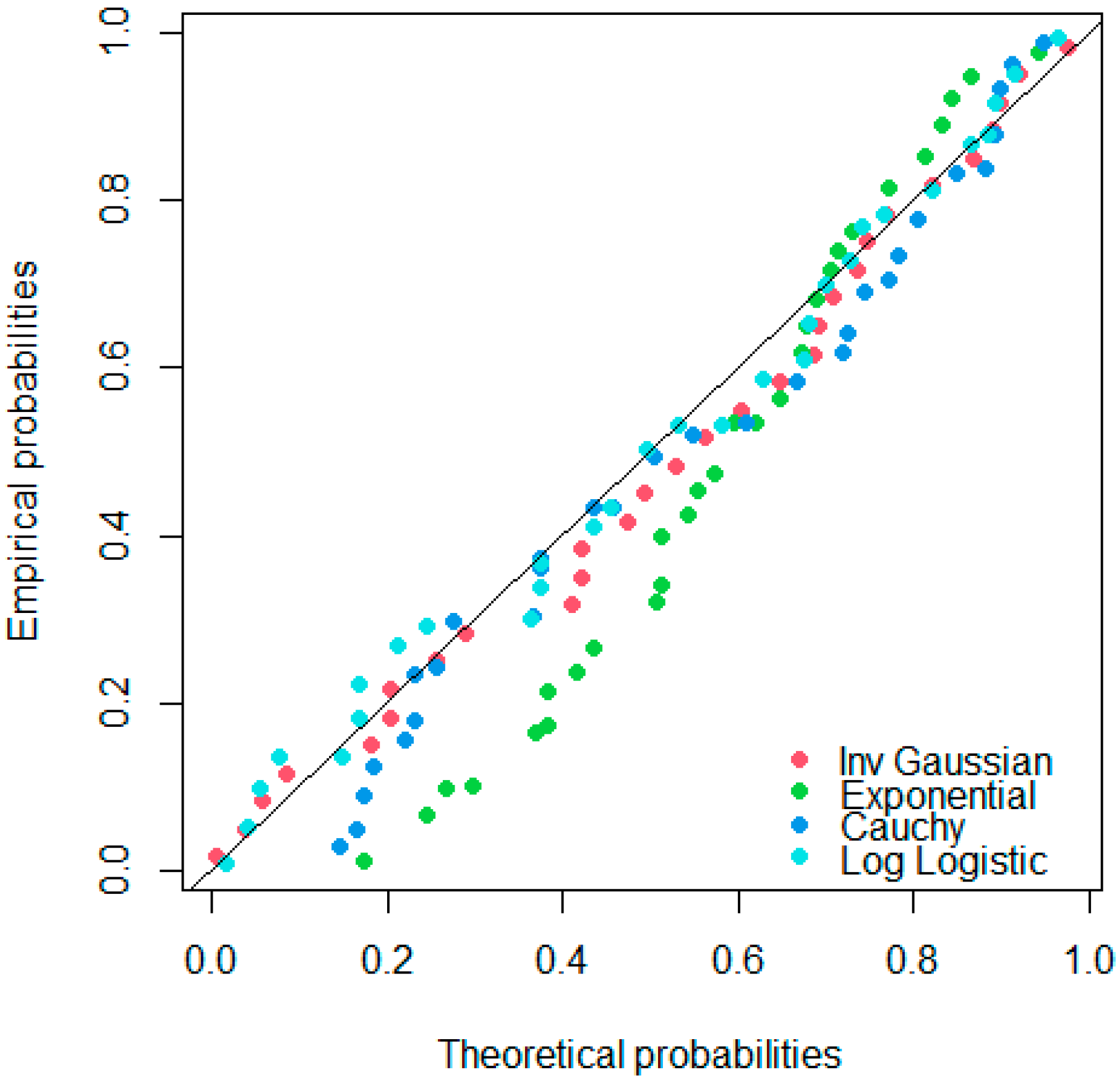
30	0.320	4.750	1.470	1.675	1.1447	1.0006

summarizes the descriptive statistics. The mean and standard deviation of precipitation are 1.675 and 1, respectively. Four candidate distributions—exponential, Cauchy, log-logistic, and inverse Gaussian—are fitted to the dataset. The results, summarized in

Table 8. Maximum likelihood estimates, goodness-of-fit testing, and AIC for the March precipitation dataset.

Distribution	Estimates	Chi-Squared Statistic	p-Value	AIC
Exponential	$\hat{\mathit{\theta }}=0.5970$	9.0049	0.1088	92.9487
Cauchy	$\hat{\mathit{\theta }}=\left(1.4251,\hspace{0.33em}0.5457\right)$	3.6964	0.4486	94.8484
Log-logistic	$\hat{\mathit{\theta }}=\left(2.7880,\hspace{0.33em}1.4407\right)$	2.5873	0.6290	81.8615
Inverse Gaussian	$\hat{\mathit{\theta }}=\left(1.6749, 3.5840\right)$	2.5662	0.6328	81.2077

, indicate that the fitted inverse Gaussian distribution has the highest p-value and the lowest Akaike information criterion (AIC), suggesting that it is the most suitable for this dataset. The estimated mean and shape parameters for the inverse Gaussian distribution are 1.675 and 3.584, respectively. From Figure 3, which displays the probability plot, it is evident that the points of the log-logistic and inverse Gaussian distributions align more closely with the diagonal line compared to the exponential and Cauchy distributions.

The 95% confidence intervals for the March precipitation dataset are computed using formulas (9), (10), (11), (15), and (23) for the PL, RPL, WRPLO, WPL, and WRPLE methods, respectively. Observation of the interval lengths in

Table 9. 95% confidence intervals for the means of the March precipitation dataset.

Interval	95% Confidence Interval	Interval Length
Existing intervals:
PL	$\left(1.3371, 2.2413\right)$	0.9042
RPL	$\left(1.3392, 2.2587\right)$	0.9195
WRPLO	$\left(1.3457, 2.2175\right)$	0.8718
Proposed intervals:
WPL	$\left(1.2652, 2.0847\right)$	0.8197
WRPLE	$\left(1.3277, 2.2682\right)$	0.9405

indicates that the results align with the simulation study. This study found that WPL typically produces shorter intervals compared to WRPLE, while both PL and RPL generally fall between these two in terms of interval length.

7. Conclusions

The mathematically derived WPL and WRPLE intervals have a closed form, making them easy for users to calculate for a given dataset. Simulation studies show the WRPLE interval provides a coverage probability close to 0.95, the nominal confidence level, compared to other intervals. For large sample sizes (at least 30), WRPLE and WRPLO are comparable, but WRPLE is superior for small sample sizes. The WPL, however, seems to have lower performance relative to WRPLE and other existing intervals in many cases; this implies that reparameterization is essential for constructing Wald-type confidence intervals. Additionally, as sample size increases, coverage probability improves for all interval types.

Future research could explore the simultaneous confidence interval construction for both parameters of the IG distribution. Additionally, there is potential to focus on other characteristics as parameters of interest, such as the variance of the IG distribution. This could broaden the applicability of confidence intervals in various statistical contexts. Another significant direction for future work includes developing software packages to facilitate the practical application of these intervals, enhancing their usability in statistical analysis.

References

- Folks, J.L.; Chhikara, R.S. The Inverse Gaussian Distribution and Its Statistical Application—A Review. J. R. Stat. Soc. Ser. B Methodol. 1978, 40, 263–289. [Google Scholar] [CrossRef]
- Schrödinger, E. Theory of Parabolic and Rising Experiments on Particles with Brownian Motion. Phys. Z. 1915, 16, 289–295. [Google Scholar]
- Wald, A. Sequential Analysis; Wiley: New York, NY, USA, 1947. [Google Scholar]
- Wise, M.E. Skew Distributions in Biomedicine Including Some with Negative Powers of Time. In A Modern Course on Statistical Distributions in Scientific Work; Patil, G.P., Kotz, S., Ord, J.K., Eds.; NATO Advanced Study Institutes Series; Springer: Dordrecht, The Netherlands, 1975; Volume 17. [Google Scholar]
- Onar, A.; Padgett, W.J. Accelerated Test Models with the Inverse Gaussian Distribution. J. Stat. Plan. Inference 2000, 89, 119–133. [Google Scholar] [CrossRef]
- Jain, R.K.; Jain, S. Inverse Gaussian Distribution and Its Application to Reliability. Microelectron. Reliab. 1996, 36, 1323–1335. [Google Scholar] [CrossRef]
- Barndorff-Nielsen, O.E.; Shephard, N. Modelling by Lévy Processes for Financial Econometrics. In Lévy Processes; Barndorff-Nielsen, O.E., Resnick, S.I., Mikosch, T., Eds.; Birkhäuser: Boston, MA, USA, 2001. [Google Scholar]
- McCarthy, M. Bayesian Methods for Ecology; Cambridge University Press: Cambridge, UK, 2007. [Google Scholar]
- Chankham, W.; Niwitpong, S.; Niwitpong, S. Measurement of Dispersion of PM 2.5 in Thailand Using Confidence Intervals for the Coefficient of Variation of an Inverse Gaussian Distribution. PeerJ 2022, 10, e12988. [Google Scholar] [CrossRef] [PubMed]
- Hougaard, P. Frailty Models for Survival Data. Lifetime Data Anal. 1995, 1, 255–273. [Google Scholar] [CrossRef] [PubMed]
- Lai, C.-D.; Xie, M. Stochastic Ageing and Dependence for Reliability, 1st ed.; Springer: New York, NY, USA, 2006. [Google Scholar]
- Krbálek, M.; Hobza, T.; Patočka, M.; Krbálková, M.; Apeltauer, J.; Groverová, N. Statistical Aspects of Gap-Acceptance Theory for Unsignalized Intersection Capacity. Physica A Stat. Mech. Appl. 2022, 594, 127043. [Google Scholar] [CrossRef]
- Fisch, K.; Schwalger, T.; Lindner, B.; Herz, A.V.M.; Benda, J. Channel Noise from Both Slow Adaptation Currents and Fast Currents Is Required to Explain Spike-Response Variability in a Sensory Neuron. J. Neurosci. 2012, 32, 17332–17344. [Google Scholar] [CrossRef]
- Stein, A.J.; Lindsey, J.K. Statistical Analysis of Stochastic Processes in Time. Environ. Ecol. Stat. 2006, 13, 247–248. [Google Scholar]
- Punzo, A. A New Look at the Inverse Gaussian Distribution with Applications to Insurance and Economic Data. J. Appl. Stat. 2019, 46, 1260–1287. [Google Scholar] [CrossRef]
- Tweedie, M.C.K. Statistical Properties of Inverse Gaussian Distributions. II. Ann. Math. Statist. 1957, 28, 696–705. [Google Scholar] [CrossRef]
- Hougaard, P. Univariate Survival Data. In Analysis of Multivariate Survival Data. Statistics for Biology and Health; Springer: New York, NY, USA, 2000. [Google Scholar]
- Davidson, R.; MacKinnon, J.G. Estimation and Inference in Econometrics; Oxford University Press: New York, NY, USA, 1993. [Google Scholar]
- Martin, V.; Hurn, S.; Harris, D. Econometric Modelling with Time Series: Specification, Estimation and Testing; Cambridge University Press: Cambridge, UK, 2013; p. 138. [Google Scholar]
- Rohde, C.A. Introductory Statistical Inference with the Likelihood Function, 1st ed.; Springer: London, UK, 2014. [Google Scholar]
- Kummaraka, U.; Srisuradetchai, P. Interval Estimation of the Dependence Parameter in Bivariate Clayton Copulas. Emerg. Sci. J. 2023, 7, 1478–1490. [Google Scholar] [CrossRef]
- Pawitan, Y. In All Likelihood: Statistical Modelling and Inference Using Likelihood; Clarendon Press: Oxford, UK, 2001. [Google Scholar]
- Murphy, S.A.; van der Vaart, A.W. On Profile Likelihood. J. Am. Stat. Assoc. 2000, 95, 449–465. [Google Scholar] [CrossRef]
- Arefi, M.; Mohtashami Borzadaran, G.R.; Vaghei, Y. A Note on Interval Estimation for the Mean of Inverse Gaussian Distribution. SORT 2008, 32, 49–56. [Google Scholar]
- Srisuradetchai, P. Simple Formulas for Profile- and Estimated-Likelihood Based Confidence Intervals for the Mean of Inverse Gaussian. J. KMUTNB 2017, 27, 467–479. (In Thai) [Google Scholar]
- Díaz-Francés, E. Simple Estimation Intervals for Poisson, Exponential, and Inverse Gaussian Means Obtained by Symmetrizing the Likelihood Function. Am. Stat. 2016, 70, 171–180. [Google Scholar] [CrossRef]
- Srisuradetchai, P. Using Re-Parametrized Profile Likelihoods to Construct Wald Confidence Intervals for the Mean of Inverse Gaussian Distribution. In Proceedings of the 19th National Graduate Research Conference, Khon Kaen University, Khon Kaen, Thailand, 9 March 2018. (In Thai). [Google Scholar]
- Lu, W.; Shi, D. A New Compounding Life Distribution: The Weibull–Poisson Distribution. J. Appl. Stat. 2012, 39, 21–38. [Google Scholar] [CrossRef]