Challenges of Engineering Applications of Descriptive Geometry

Abstract

Descriptive geometry has indispensable applications in many engineering activities. A summary of these is provided in the first chapter of this paper, preceded by a brief introduction into the methods of representation and mathematical recognition related to our research area, such as projection perpendicular to a single plane, projection images created by perpendicular projection onto two mutually perpendicular image planes, but placed on one plane, including the research of curves and movements, visual representation and perception relying on a mathematical approach, and studies on toothed driving pairs and tool geometry in order to place the development presented here among them. As a result of the continuous variability of the technological environment according to various optimization aspects, the engineering activities must also be continuously adapted to the changes, for which an appropriate approach and formulation are required from the practitioners of descriptive geometry, and can even lead to improvement in the field of descriptive geometry. The imaging procedures are always based on the methods and theorems of descriptive geometry. Our aim was to examine the spatial variation in the wear of the tool edge and the machining of the components of toothed drive pairs using two cameras. Resolving contradictions in spatial geometry reconstruction research is a constant challenge, to which a possible answer in many cases is the searching for the right projection direction, and positioning cameras appropriately. A special method of enumerating the possible infinite viewpoints for the reconstruction of tool surface edge curves is presented in the second part of this paper. In the case of the monitoring the shape geometry, taking into account the interchangeability of the projection directions, i.e., the property of symmetry, all images made from two perpendicular directions were taken into account. The procedure for determining the correct directions in a mathematically exact way is also presented through examples. A new criterion was formulated for the tested tooth edge of the hob to take into account the shading of the tooth next to it. The analysis and some of the results of the Monge mapping, suitable for the solution of a mechanical engineering task to be solved in a specific technical environment, namely defining the conditions for camera placements that ensure reconstructibility are also presented. Taking physical shadowing into account, conclusions can be drawn about the degree of distortion of the machined surface from the spatial deformation of the edge curve of the tool reconstructed with correctly positioned cameras.

1. Introduction

One of the objectives of this paper is to highlight the constant challenges of engineering communication, which can sometimes be accompanied by the need for a new aspect-based approach to the descriptive geometry, which forms a basis for engineering communication. Today’s technological progress requires the continuous renewal of knowledge necessary for the operation and development of more modern devices, primarily engineering knowledge in particular. Engineering ideas are translated into technical drawings based on descriptive geometry, independent of the device, but always on the 2D plane with a mutually clear correspondence between the elements of the 3D space and those of the 2D plane (supplemented by additional informative data).

One of the many challenges of descriptive geometry is the recognition, highlighted by Stachel [1], that the essence of descriptive geometry is not that the drawings are “made by hand”, because even Gaspar Monge, from whom descriptive geometry originates, did not refer to it as being an essential part of it [2]; in summary, it can be stated that a manual drawing is not a feature of descriptive geometry. We should not be fooled by the fact that even with the introduction of 3D-CAD/CG, the essence of hand-drawing descriptive geometry is that one of the most useful ways to facilitate understanding and firmly fix memories is to simultaneously use the senses, namely the “eyes” and motor organs, such as the “hand”, since these things are connected in a similar way when acquiring any type of knowledge [3].

Visual perception and its modeling, control and learnability have been investigated by neuroscience research. The connection between visual perception and consciousness has also been analyzed [4]. According to Stachel, “Descriptive Geometry is the interplay between the 3D situation and its 2D representation, and between intuitive grasping and rigorous logical reasoning” [1]. Therefore, in addition to the theory of projection, descriptive geometry also includes the techniques of modeling curves and surfaces, as well as the intuitive approach of elementary differential geometry and 3D analytical geometry. Descriptive geometry has two main purposes. Firstly, it provides a method of imaging 3D objects, and secondly it facilitates the recognition of body shapes by their exact description, as well as to derive truths and mathematical regularities arising from their shape and position.

Orthogonal projection is the most commonly used method for mapping 3D space onto a 2D plane.

When projecting physical “real” surfaces of Euclidean space onto a plane using orthogonal projection, elevation data are usually also supplied. Cartography, geodesy, mining, road and railway construction and river regulation, as well as solving certain tasks in forestry require a special representation method of descriptive geometry, the one view representation with the indication of elevations [5].

In earth sciences, cartographic data are supplemented with a large amount of information during the recording and analysis of the results of seismic monitoring measurements [6]. The field observations of topography are supplemented with measurement data require global optimization tools and robust statistical techniques to manage the data and extract additional information in order to build an extended groundwater flow model of the research area [7]. The topographic representation of the complex surface of the terrain is the basis of digital elevation models DEMs in the professional terminology. In this case, there is a risk of losing a large amount of detailed topographical information due to traditional interpolation methods. To avoid this, a new method based on sliding windows has been proposed to improve the resolution of DEMs [8].

In another research area, the microtopography of machined surfaces is measured using sensor technology, based on metric orthogonal projection. The effect of the use of a round milling insert on the surface topography was studied at different cutting speeds. The surface roughness could be determined from the trace of the tool geometry on the workpiece taking into account the kinematics which in turn depends on the different cutting speed and possibly other process characteristics as well. By changing the surface roughness, the friction between the motion-transmitting machine parts, as well as the wear and corrosion resistance, and the creep strength of the parts can be influenced [9]. Although the evaluation of surface quality is applied with 2D parameters during engineering practice, the analysis of the microtopography of the curved surfaces with a 3D optical microscope also provides information about the integrity of the surface, for which it is also necessary to determine the appropriate viewpoints [10]. In an additional area of research, finite element tests of a 2D cross-section are carried out for the analysis of 3D cylindrical industrial facilities and the physical phenomena occurring in them, for example also in thermal models prepared for individual industrial applications. In a lumped heat capacity model prepared for transient heat convection analysis in cross-air flow, the Finite Element Analysis simulations used with the ANSYS Fluent code are also performed in 2D sections, the results of which also show that the geometric shape of the 2D section has a clear effect on heat loss as well [11].

Among the types of multi-view representation, the two-view Monge representation is the most frequently used during engineering activities [12]. The most important informational value of the descriptive geometric procedures is that the dimensions and location of the spatial shapes can be clearly determined (provided with additional information, such as regarding their movement) [13].

Monge realized that descriptive geometry has a great importance in the field of engineering, and the treatment of space in this way also gives rise to the study of the properties of curves. Though most of the lines in any industrially created objects are the straight lines, using of the curves is so frequently required that the designer should always be prepared to apply them with confidence and competence. Facility in handling curved lines can come only as effect of the accurate knowledge of the general principles for governing of the curve generation or from practice on some concrete cases.

One of Monge’s most talented students was Theodore Olivier, who is primarily known for creating three-dimensional moving models of descriptive geometric processes. Olivier’s moving models led to the study of movement transmission by means of descriptive geometry, which provided the basis for differential geometric analyses [14]. The time stability of steps leading to Olivier’s results can also be excellently observed in the typical case of the generation of 2D curves, according to which the interpretation of the synthetic geometric evolution of the roulettes is the basis of their analytical definition. For the computer 2D graphic representation and 2D animation of roulettes, their analytical formulation based on their synthetic geometric analysis is required, which leads all the way to the topic of related surface pairs and the gearing [15].

According to Olivier’s theory, an imaginative collaboration between the physical implementation of the synthetic geometric evolution of roulettes and the virtual display of its analytical determination can be realized by operating drawing educational robots combined with the Desmos dynamic geometry software developed for this purpose and operated with adjustable drive pairs [16]. The tooth profile of elliptical gears with a continuously variable gear ratio has a special geometry, an ellipse involute instead of the “standard” circular involute- Its 3D printed model of which was also created to support the developed process based on its mathematical geometrical definition [17]. The changing ratio noncircular gear drives are imaginative machine parts that offer a wide range of applications. In some special engineering fields, these solutions (determined by the use of transported lines of actions, resulting in variable axis distance and tooth profile [18], or even by applying the basic law of gearing, the function of alternating profile offsets at the constant axis distance was determined within certain limits [19]) can have many advantages over traditional solutions. In the field of novel approaches to the design of space curves corresponding to the most diverse boundary conditions, such as the optimization of the movement paths of robot arms, the industry constantly floods researchers with challenges. An up-to-date hybrid algorithm has been developed in its geometrically also new approach, which determine that trajectory of a robot arm with the lowest cycle time between two given points, avoiding obstacles from a space of possible ones [20].

The determination of the twisting, which replaces the movement between two different positions of the motion trajectories, was also inserted into the constructive geometric model developed for the investigation of kinematic drive pairs with the descriptive geometrical methods [21]. Following Theodore Olivier’s idea on the practical application of theoretical mathematical research should be tuned to physical realizations, the definition and visualization of the time-like axis of helical hypersurfaces [22] is also a possible connection point between mathematics and engineering research fields.

In the case of machining a spiroid worm with axis adjustment, the effectiveness of the knowledge of the momentary torsion axis and the correct choice of the descriptive geometrical projections is demonstrated, among other things, by the use of views following the motion transmission processes when determining the drive pin profile for eliminating the thread pitch fluctuation. In the case of machining with traditional thread grinding, the generatrix of the reference cone of the conical worm must be placed onto the path of the thread grinder, namely its axis must be set with the semi-angle of the reference cone, with a drive pin converting the direction of motion. The momentary screw axes of the time-dependent relative motion of interconnected space systems allow us to infer the momentary poles in the corresponding views. In the corresponding views, the radius drawn from the momentary pole to the moving point is perpendicular to the trajectory tangent. By selecting the appropriate length of the tangent, the drive pin profile can be constructed, namely accurately calculated, in an explicit form [23].

By defining the spatial kinematics method for following the operation of the drive pairs with mathematical precision, in the mathematical model built on properly interpreted views, the tooth surface points of the gear wheel connected to the Archimedean worm can be generated with the numerical procedure developed for this purpose, which is a mathematical geometrical modeling of the gear tooth surface [24].

The second of the two main purposes of descriptive geometry is to improve the mathematical visual perception of objects in three-dimensional space [25]. For the modeling procedures of the imaging of spatial objects, several concepts worthy of consideration have been created [26].

A serious challenge for applied optical research is to harmonize the operation of optical imaging systems and the toolbox of geometric optics with mathematical formulas in such a way that, by following the imaging processes perceptible to the human eye, it helps visual recognition while also supporting the evolving of geometric awareness [27].

Several computer imaging techniques exist that simulate a critical property of human vision namely imperfection resulting from highly effective wave front aberration that vary from person to person. In addition to existing vision simulation techniques, there are many new challenges in rendering algorithms to simulate aberrant human vision [28]. An exact solution for connecting visualization with conscious geometric interpretation is computer-enhanced descriptive geometry (CeDG), a modern scientific approach to solving and creating computer modelling of three-dimensional (3D) geometric systems through descriptive geometry procedures. The contribution of the new approach to the field of science is the inheritance of the laws of projective geometric invariants bearing the signs of duality, which ensure reliability and accuracy at the same time. To support the theoretical foundations, the procedure has been also presented by determining the intersection curve of two surfaces in a parametric implicit functional form [29].

A special form of modelling was published during a promising research of three-dimensional virtual data visualization tools and methods. The relationship of the different life formats that can be used as input data was represented using a sphere-based visualization technique, the ends of the nodes were placed on the sphere and the relationships were displayed with tube-like surfaces [30].

A number of concepts have been created for modelling spatial objects, which are widely recognized [31]. The relationships of the different file formats that can be used as input data were represented using a sphere-based visualization technique; the ends of the nodes were placed on the sphere with the relationships displayed as tube-like surfaces [32].

During the creation of a model of an existing physical 3D object, one of the many problems that arise can be classified as difficulties associated with the geometric accuracy of the data and the visualization quality of the result. The main reason mentioned for modelling problems is that none of the current computer-aided design (CAD) software packages have sufficient tools to accurately map the measurement data of an object to be modelled from all the necessary aspect. For this reason, the process of 3D modelling consists of a relatively large proportion of manual work, such as when arranging individual points and in the case of approximation of curves and surfaces. In some cases, it is necessary to generalize the model in the CAD system, which reduces the accuracy and field data quality. As a possible solution, the use of topological codes and the use of the new specific CAD services created was also proposed in a study by Bartonek and co-authors [33].

Only those with sufficient skills in descriptive geometry are able to professionally use CAD modelling programs due to communication based on views taken from descriptive geometry [34]. Just as the importance of mathematical knowledge continues to increase with the transfer of calculation work to computers, an increasingly high level of geometrical knowledge is also required to operate it increasingly sophisticated modelling software [35,36,37,38]. The spatial form imagined by the mathematical geometric definition is realized during the physical implementation (industrial production) and will be influenced by several technological and production processes related factors [39]. One possible abstract formulation of this process is mathematical geometric modelling [40]. A number of technological and processing parameters are added to the mathematical geometric parameters of the surfaces of parts during production, resulting in deviation from the originally defined ideal surface.

Among other things, production geometry focuses on the theory of the geometry of tools that machine the industrial parts, the examination and analysis of the surface deviation of the machined parts compared to the geometrically defined surfaces, and the development of the related manufacturing processes, all which are based on descriptive geometry. For production geometry challenges, an acceptable answer must be given every time which, while obviously limited by the available technologies and resources, should nevertheless result in the smallest deviations possible between the manufactured and the mathematically defined surfaces.

Olivier’s research was unique for a long time in the two main fields of the tooth-generation theory of mechanisms, teeth meshing conditions and manufacturing geometry. In his work published in 1842, he even separated the tooth surface theory from the analytical (mathematical) and enveloping (geometrical) methods [41]. According to his interpretation, the question of tooth meshing in its entirety belongs to descriptive geometry. According to Gohman, tooth theory is a special area of the discipline of mathematics, where researchers, in contrast to other areas of mathematics science, should only take small steps forward, always looking for the next safe point.

The essential role both scientists played in creating the foundations of today’s spatial tooth theory is indisputable [40]. In worm gear drive research, a “Worm Scientific School” has been established at the University of Miskolc, producing 13 defended doctoral dissertations. Synthetic geometry supported by analytical geometry was applied to analyze the structure and operation of technical constructions, such as for the production geometry development of the components of conical and cylindrical worm gear drive pairs during the creation of the constructive geometric model. The mathematical geometric generation of helicoidal surfaces in the constructive geometric model sets the direction for the development regarding the correct machining of cylindrical and conical worms and that of their production geometry [42].

A typical example of the production geometry examinations was aimed at comparing the modified geometric parameters of spur gears having normal involute teeth and the related technological parameters were compared with the manufacturing parameters to reveal the correlations in order to advance the technological design [43]. In the industrial applications, instead of the elemental toothing created by mutual enveloping, so-called profile offset toothing is often used, which can increase the load capacity and prevent malfunctions. However, since there is no solution that is favorable from all aspects at the same time for the selection of the profile shift coefficients, the basis of the decision is always a careful consideration of the operating conditions and the expected damages. However, with appropriate objective functions, it is possible to take into account several aspects at the same time to choose the profile shift coefficient, including the suitable lubricating film thickness, linear wear, gear tooth bending stress, and Hertzian stress, which affect tooth damage and operating conditions [44].

The production geometry of the components of the conical worm gear drives is a serious challenge, especially in connection with the analysis of the undercutting. The boundary line of the curvature interference has been investigated for the tooth surface of a gear enveloped by a conical helicoid surface. By analyzing the effect of the main design parameters on the curvature interference, the positions on the concave tooth surface of the gear with a chance of undercutting were delimited [45].

A detailed analysis of the contact between the worm gear tooth surfaces of the worm gear and the involute worm tooth surface can be made by applying the mathematical model for the dynamical analysis of the involute cylindrical worm gear drive tests regarding the load. Using the torsional oscillating dynamical model, which clearly follows the geometric interpretation, the influence of the geometric parameters the calculation of deviations, velocities or accelerations at any random node of the dynamic model can be investigated, and together with other dynamic characteristics the position of the lubricant in the contact zone between the tooth surfaces can be analyzed, because if it is displaced, metal contact and wear occur [46]. The geometry of worm teeth has a significant effect on the design of the lubricating wedge, which is important in terms of increasing wear resistance, service life and efficiency [47].

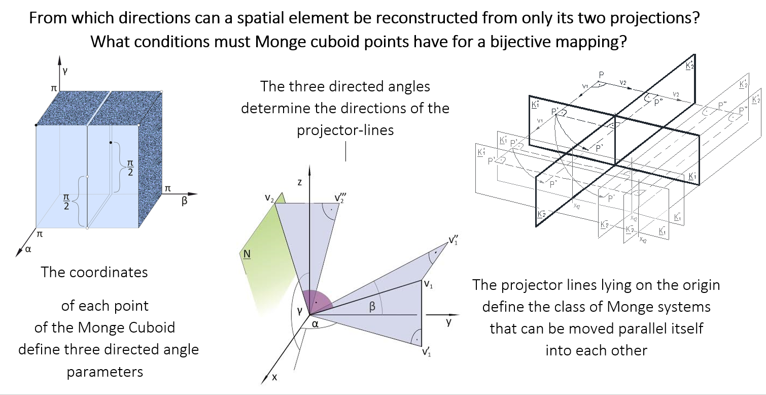
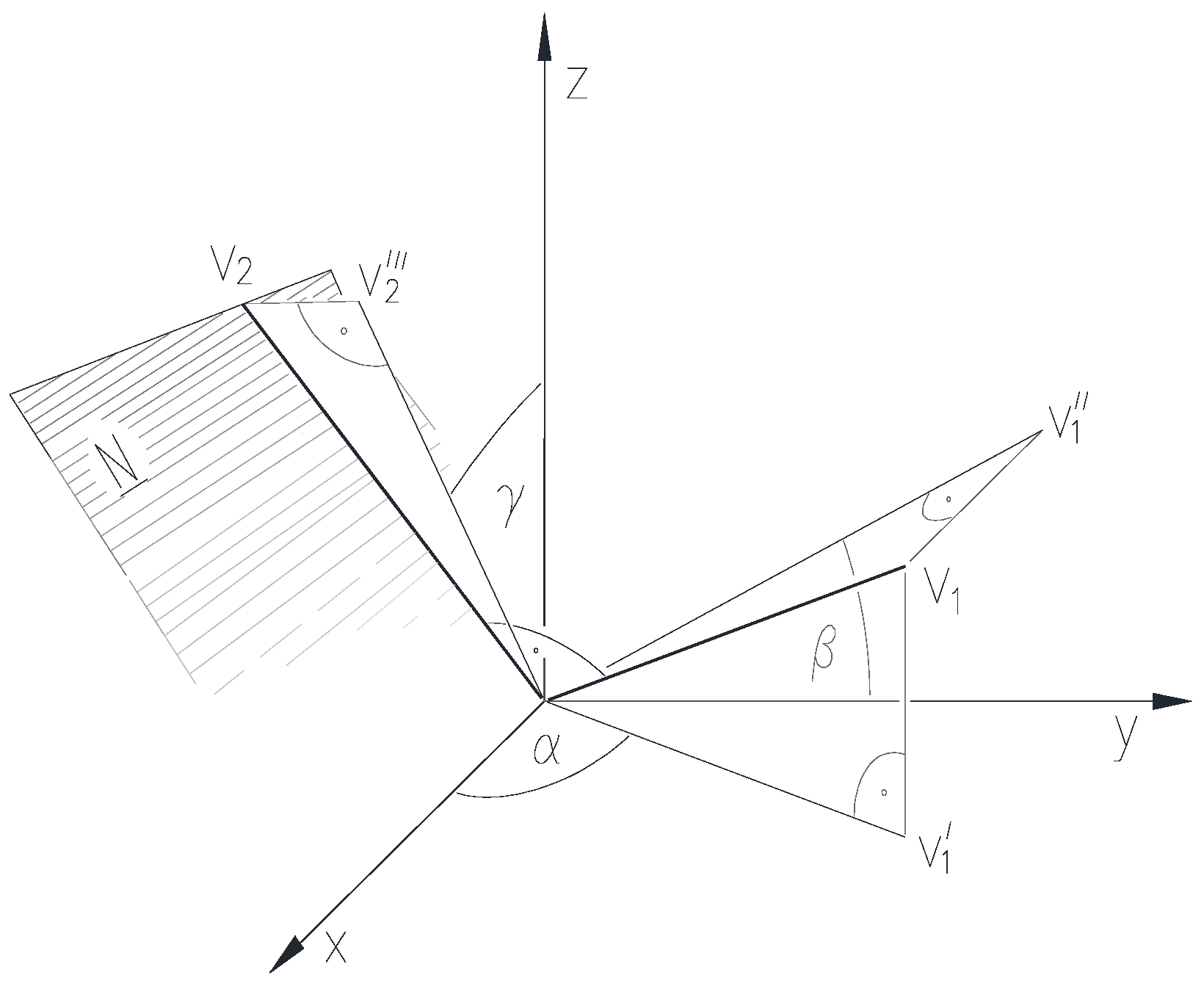
The operating surfaces of drive pair elements are produced by enveloping the surface of the machining tool surface. The increase in the variety of technological solutions also requires the continuous adaptation and investigation of tool geometry. And the development of tool geometry itself carries the geometrical challenges of descriptive geometry. The idea of the theoretical analysis of the descriptive geometry was related to the wear test of the tool, which was carried out by our Worm Scientific Research Group in the DifiCAD Engineering Office, which has a cooperation agreement with the University of Miskolc. A special approach to ensuring reconstruction from digitized images was proposed in the field of tool geometry research related to our Worm Scientific Research Group. Measuring the wear of the cutting edge of the tool with only one CCD (Charge-coupled Device) camera and a distance meter placed next to its lens already gave rise to doubts about the accuracy of the measurement [48]. It is preferable in terms of geometric accuracy to test the cutting-edge wear based on the true-to-size Monge representation with images taken with two CCD cameras positioned at right angles to each other, as can be seen in Figure 1.

For a given cutting edge curve, the image plane system can be defined in an infinite number of ways.

Definition 1.

An image plane system {K₁, K₂} consisting of mutually perpendicular image planes together with the first projector line v₁ perpendicular to the first image plane, and the second projector line v₂ perpendicular to the second image plane defines a Monge projection.

Hereinafter, the statements are made using the term as defined above. Therefore, not only the image plane system, but also the Monge projection can be used for a curve g in an infinite variety of ways. The formulated task was to determine the criteria for the positions of the image plane systems of the Monge mapping relative to an object fixed in the space, to be meet so that the fixed object of the space can be clearly reconstructed only from the two projections on the image planes of the Monge representation only, without any other information [49]. The reconstructibility of the g curve does not change when the image planes are exchanged, so taking this symmetry property into account, all possibilities were considered [50].

2. Method of Ensuring the Bijectivity of Monge’s Representation by Defining the Directions of the Views

The need to investigate bijectivity has been created by the requirement to reconstruct digitized Monge images during the research work in. Spatial objects are represented by their surface edges and lines, so as a first step the examination should be limited to these. While Monge’s representation of the point is always clear if the generally known conventions are met, anomalies may arise in the practical application of descriptive geometry, for example during the reconstruction of curves, which must be consciously kept in mind. For example, neither the representation of a circle in general location nor that representation of a profile straight line is clear due to reconstruction complications, so the reconstruction in these cases is not clear from only two digitized images without additional information. For these and similar occurrences the descriptive geometry has found special clarifications to ensure bijectivity up to now. In the case of curve mapping, the reconstruction may require some additional information such as correspondence marking. To ensure the reconstruction when representation of the curves g, the appropriate placement of the image plane system was formulated as tasks, in accordance with engineering expediency.

2.1. Examining the Spatial Curve

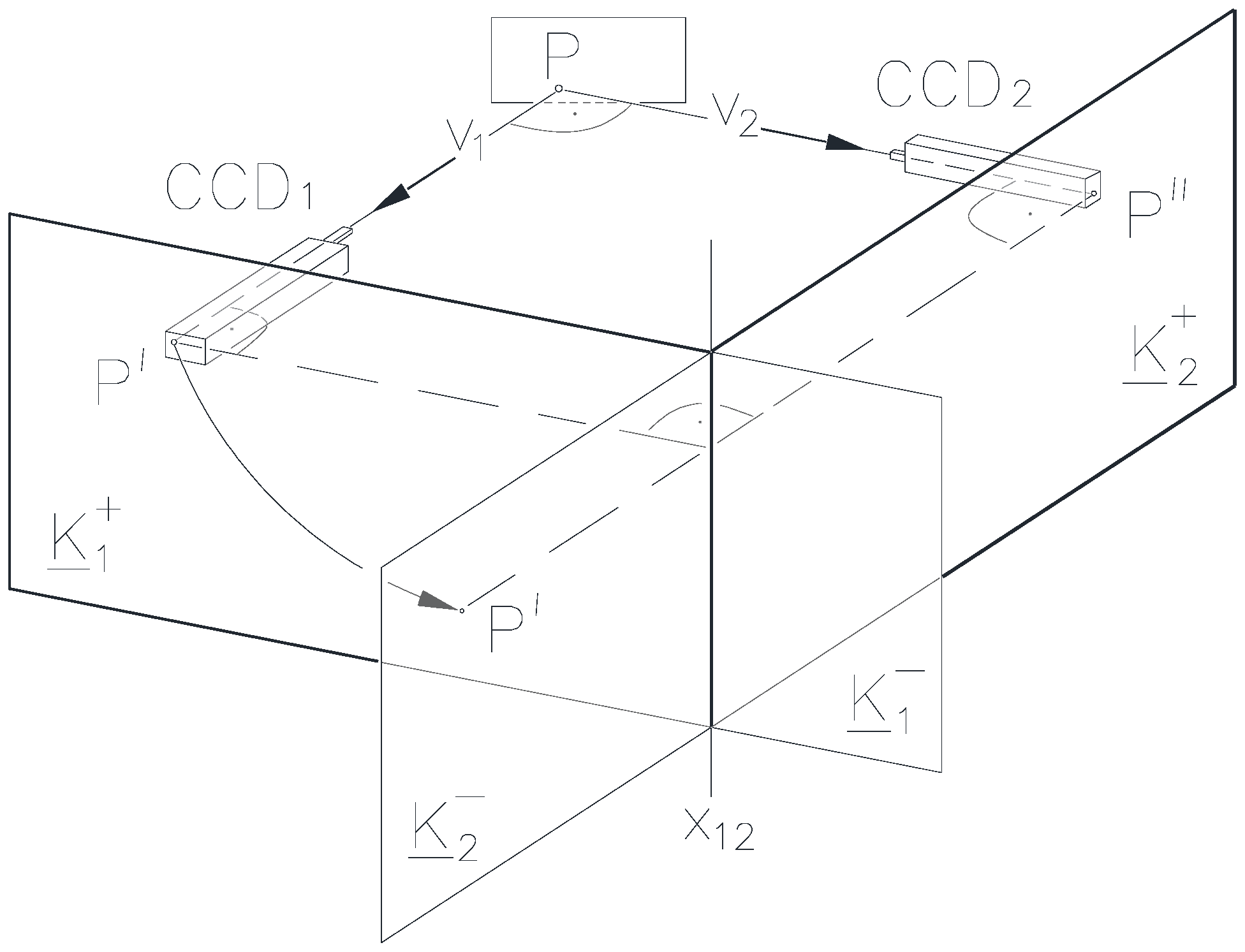
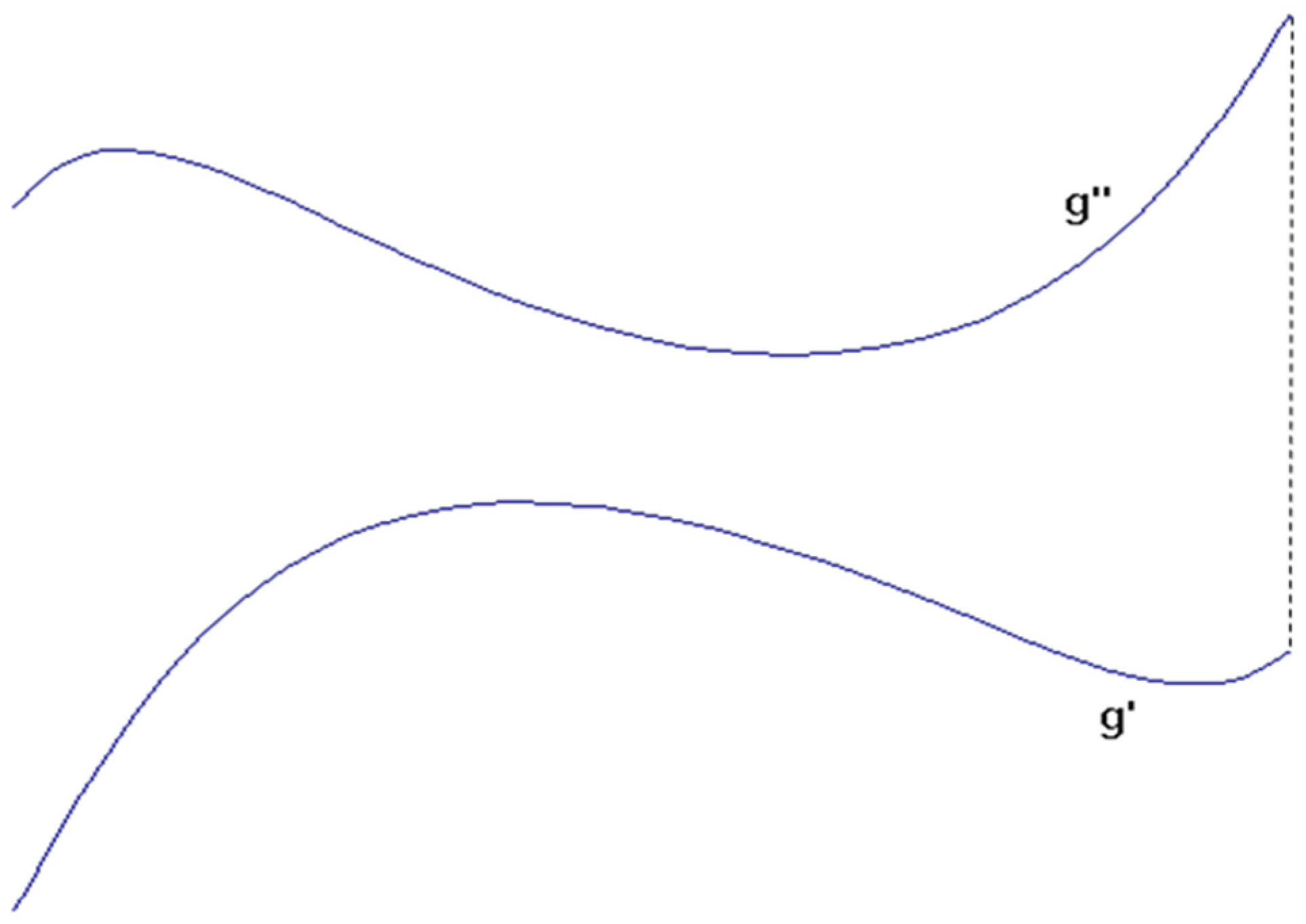
In the case of the Monge representation of the differential geometrically interpreted curve g, the coordinate planes [xy] and [yz] of a Cartesian coordinate system are fitted to the image planes K₁ and K₂ of the Monge representation, respectively. In this arrangement, the y coordinate axis will be the intersection straight line of the two image planes, namely the x₁₂ axis.

Theorem 1. 

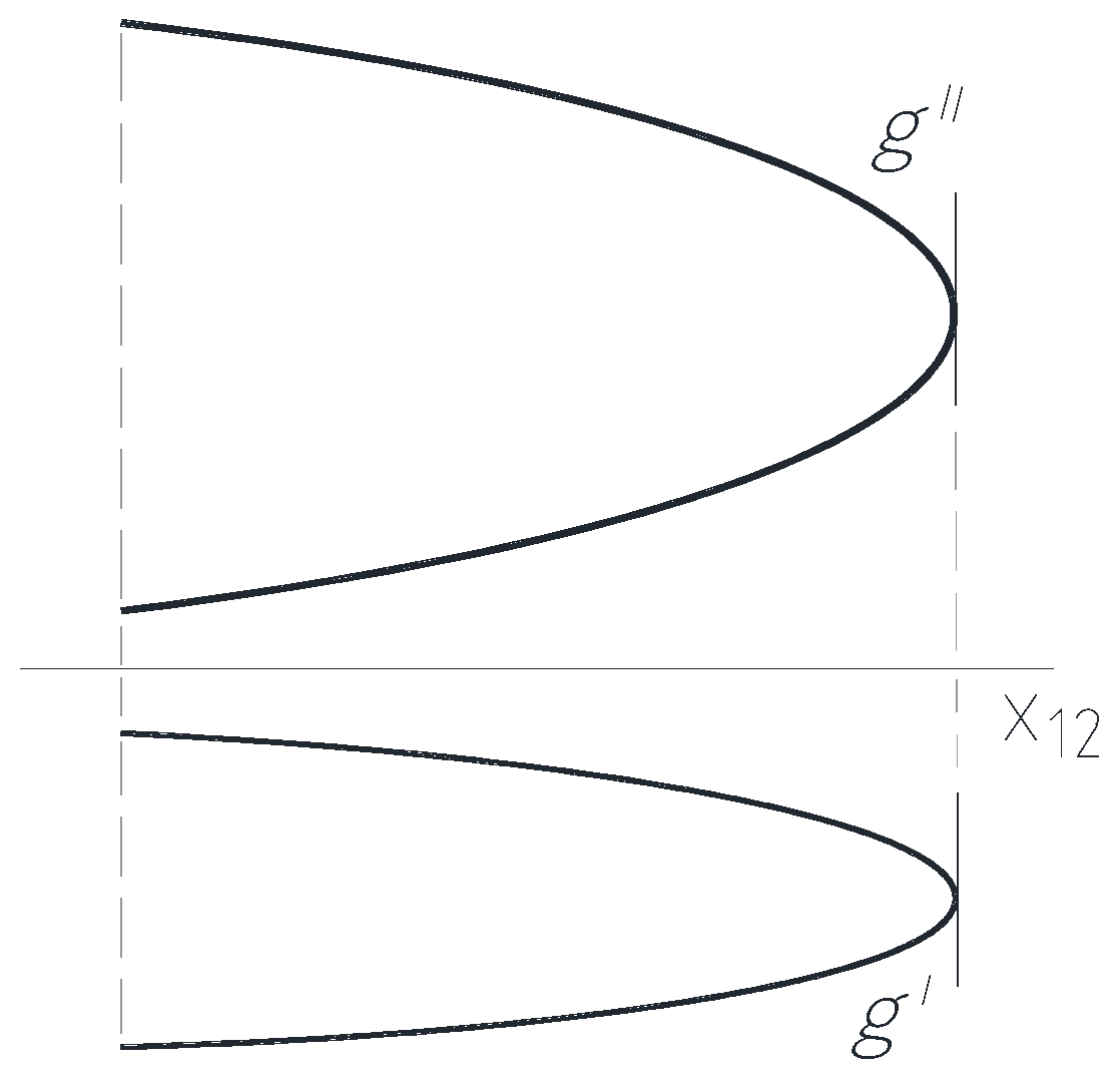
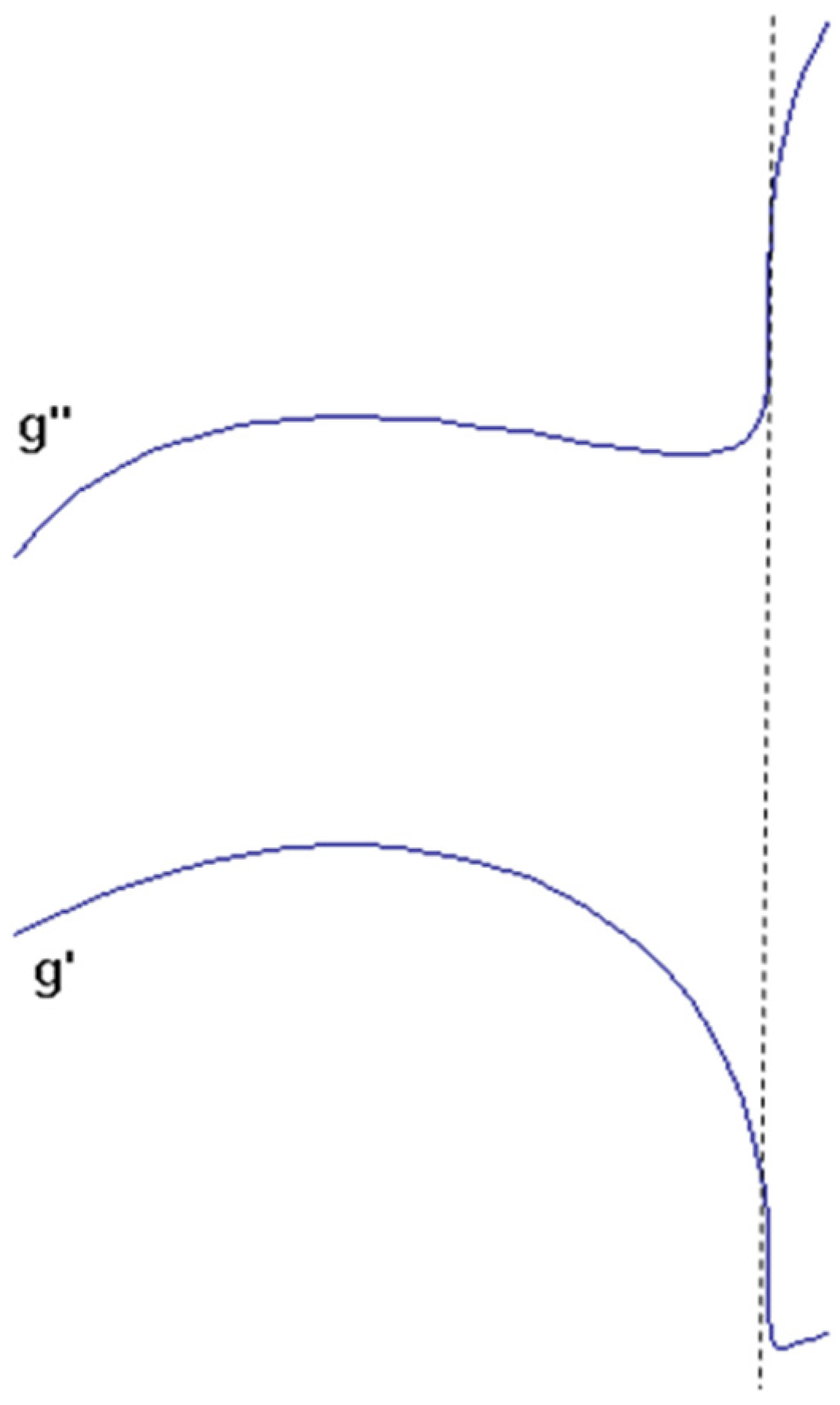
If the image curves g′ and g″ of the curve g can be described by the functions y→f₁(y) and y→f₂(y), respectively, in the corresponding Cartesian coordinate planes of the image planes, where x = f₁(y) and z = f₂(y) i.e., its points have coordinates P(f₁(y), y, f₂(y)), then any part of the curve g can be clearly reconstructed from its images.

A sketch of the curve, which can be clearly reconstructed from its projections, is shown in Figure 2.

Proof of Theorem 1. 

The function is such a subset of the Descartes product without identical first terms and no different second terms. Therefore, to one y there is assigned only one f₁(y) ≡ P′ fitting to the plane [xy] ≡ K₁ and one f₂(y) ≡ P″ fitting to the plane [yz] ≡ K₂. These lines assigning P′ and P″ to a single y value is located perpendicular to the coordinate axis y ≡ x₁₂ axis. Thus, after the merging of the image planes K₁ and K₂, the (P′, P″) forms an ordered pair of points to which only one spatial point P belongs. Therefore, any point of the curve g and thus any part of it can be clearly reconstructed. □

Corollary 1. 

If the images g′ and g″ of a curve g in the O[x, y, z] coordinate system of a Monge projection can be written separately as functions of y→f₁(y) and y→f₂(y), then no single profile plane of the Monge projection intersects more than one point each from g′ and g″ each.

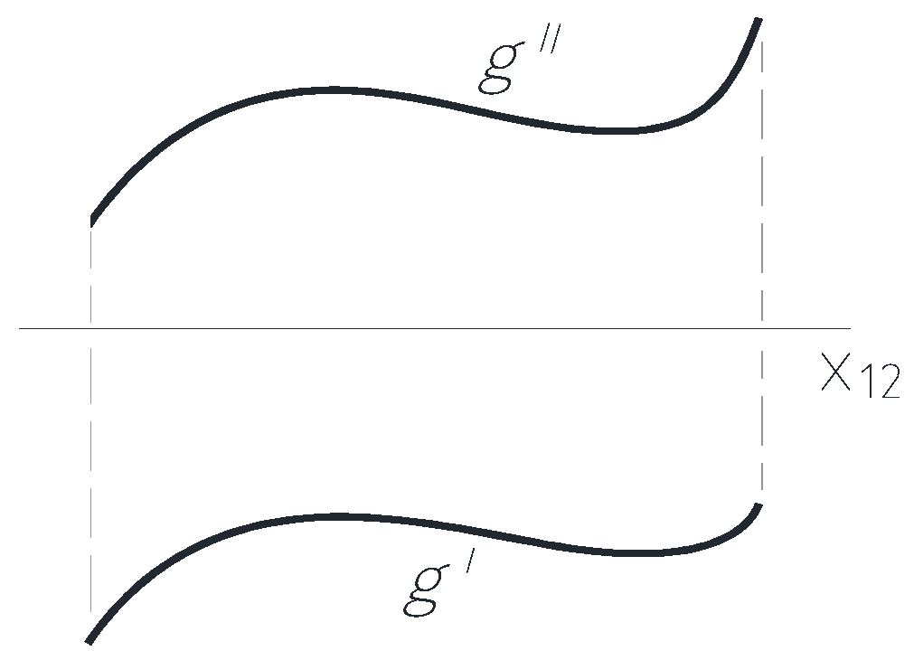
Theorem 2. 

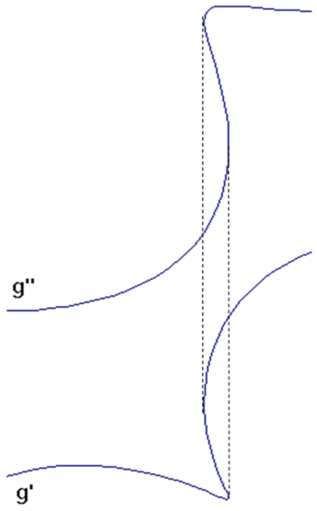
If the image curves g′ and g″ of the curve g cannot be written in the corresponding Cartesian coordinate planes as function x = f₁(y) and z = f₂(y), respectively the assignments and y→f₁(y) and y→f₂(y) are not functions, then there is a part of curve g, that cannot be clearly reconstructed from its two images.

A sketch of the curve, which cannot be clearly reconstructed from its projections without additional information, is shown in Figure 3.

Proof of Theorem 2.

Since the projected curves g′ and g″ of the spatial curve g cannot be formed as functions, but obviously they are curves, on the corresponding Cartesian coordinate planes, a single y has several f₁(y) ≡ P′ points lying on the plane [xy] ≡ K₁ and several points f₂(y) ≡ P″ lying on the plane [yz] ≡ K₂. These image points P′ and P″ fitting to a recall line perpendicular to the axis y ≡ x₁₂ can optionally be arranged to form ordered pairs of points, to which the spatial points P belong. So, there exists a point of the curve g and a neighbor of this point that cannot be reconstructed from only two images. □

Corollary 2. 

If the image curves g′ and g″ in the corresponding coordinate planes of the given Cartesian coordinate system cannot be written as functions x = f₁(y) and z = f₂(y) then

1. 

there exist profile planes of the Monge projection that intersect the curve g in more than one point, and

2. 

there is at least one profile plane tangent to g.

Theorem 3. 

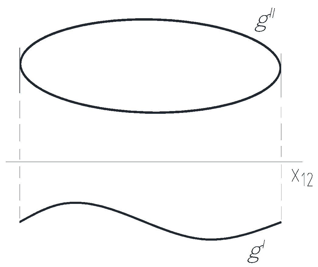
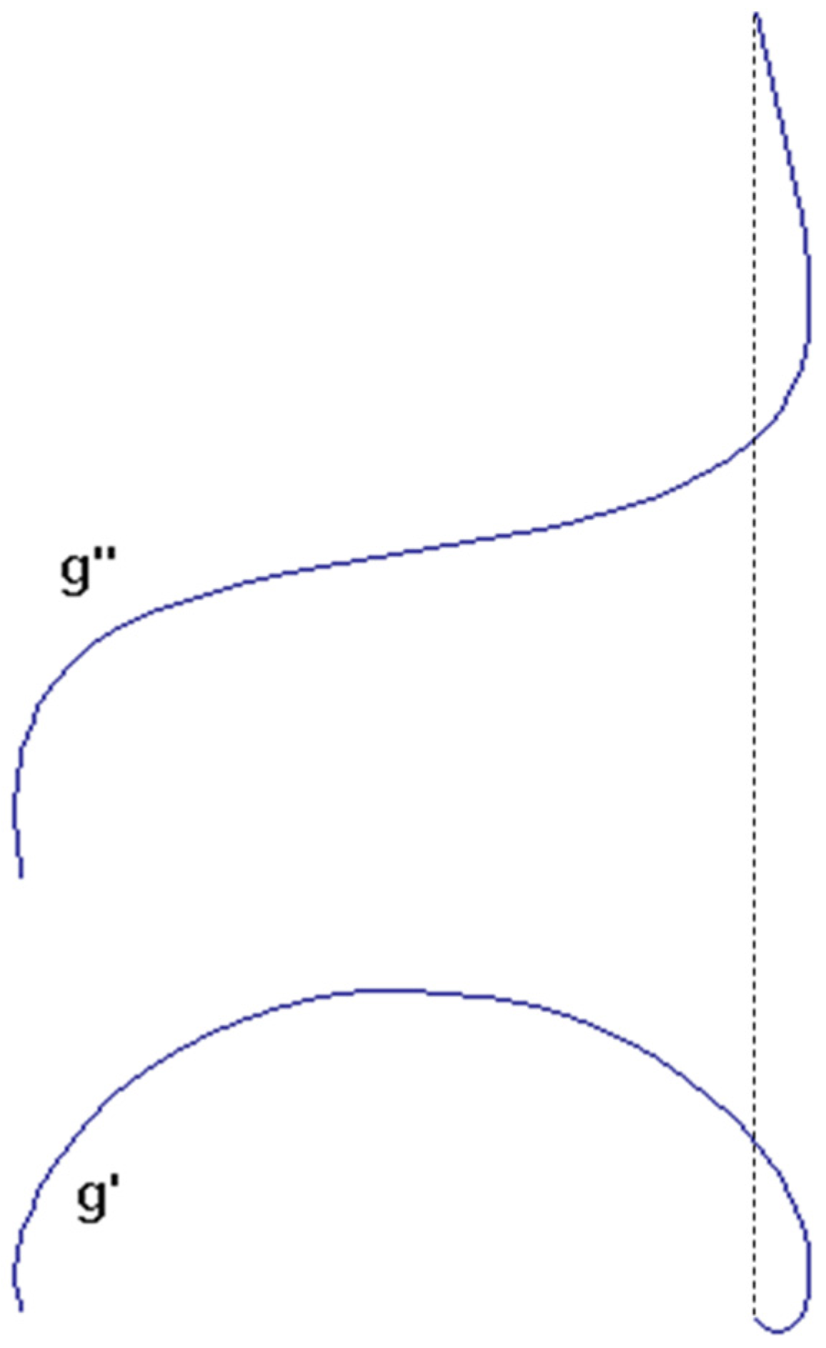
If either of the image curves g′ and g″ of the curve g cannot be written in the corresponding Cartesian coordinate plane as a function x = f₁(y) or z = f₂(y) but the other image is a double projection, and this can be written as functions z = f₂(y) or x = f₁(y), then any part of g can be clearly reconstructed from only two images.

A sketch of the projections of such a curve can be seen in Figure 4. One image of this curve cannot be written as a function on the corresponding Cartesian coordinate plane, but the other image is a double projection, that can be written as a function, so any part of the curve can be clearly reconstructed from only its two images.

Proof of Theorem 3. 

• Assume that from the image curves g′ and g″ of the curve g, g′ is a double projection, and it can be written as a function x = f₁(y), and the g″ cannot be written as a function z = f₂(y) on the corresponding Cartesian coordinate plane. In this case, a single y corresponds to a point f₁(y) ≡ P′ fitting to the plane [xy] ≡ K₁ and several points f₂(y) ≡ P″ fitting to the plane [yz] ≡ K₂. These one P′ and several P″ points located perpendicular to the y ≡ x₁₂ axis can be assigned to each other to form ordered pairs of points, to which several spatial P points belong. Thus, any point of the curve g and thus any part of it can be clearly reconstructed from only two images.
• If the image curve g″ is a double projection which can be written as a function z = f₂(y) and g′ cannot be written as a function x = f₁(y), the proof is the indices 1 and 2, as well as ′, and ″ can be done in the same way as in case 1 by exchanging the signs. □

Corollary 3. 

If either of the image curves g′ and g″ of the curve g cannot be written in the corresponding Cartesian coordinate plane as a function x = f₁(y) or z = f₂(y), but the other image is a double projection, and this can be written as a function z = f₂(y) or x = f₁(y), then there is at least one profile plane that touches g.

Theorem 4. 

If the curve g does not have a tangent parallel to the profile straight directional, then the representation of any part of the curve is bijective.

Proof of Theorem 4. 

If the curve g does not have a tangent in the profile direction, this means that the tangent at any point P₀ with parameter u₀ of its images is not in the direction of the recall line, namely the recall line intersects the examined curve in point P₀. So, there is no point P₀ of the curve g with parameter u₀, in the region of which all points P₋₁ and P₁ with parameters u₋₁ and u₁ are located on one side of the recall line of the point P₀, where u₋₁ < u₀ < u₁. This means that there is no curve segment that has two points on a recall straight line. Because each recall straight line has only one point on the curve g, any point on curve g can be reconstructed from its two images, which means that the representation of the curve is bijective. □

All of this follows from the fact that not all points of a curve can be marked with letter and comma.

2.2. Correspondence between Ordered Orthogonal Projections and Real Number Triplets

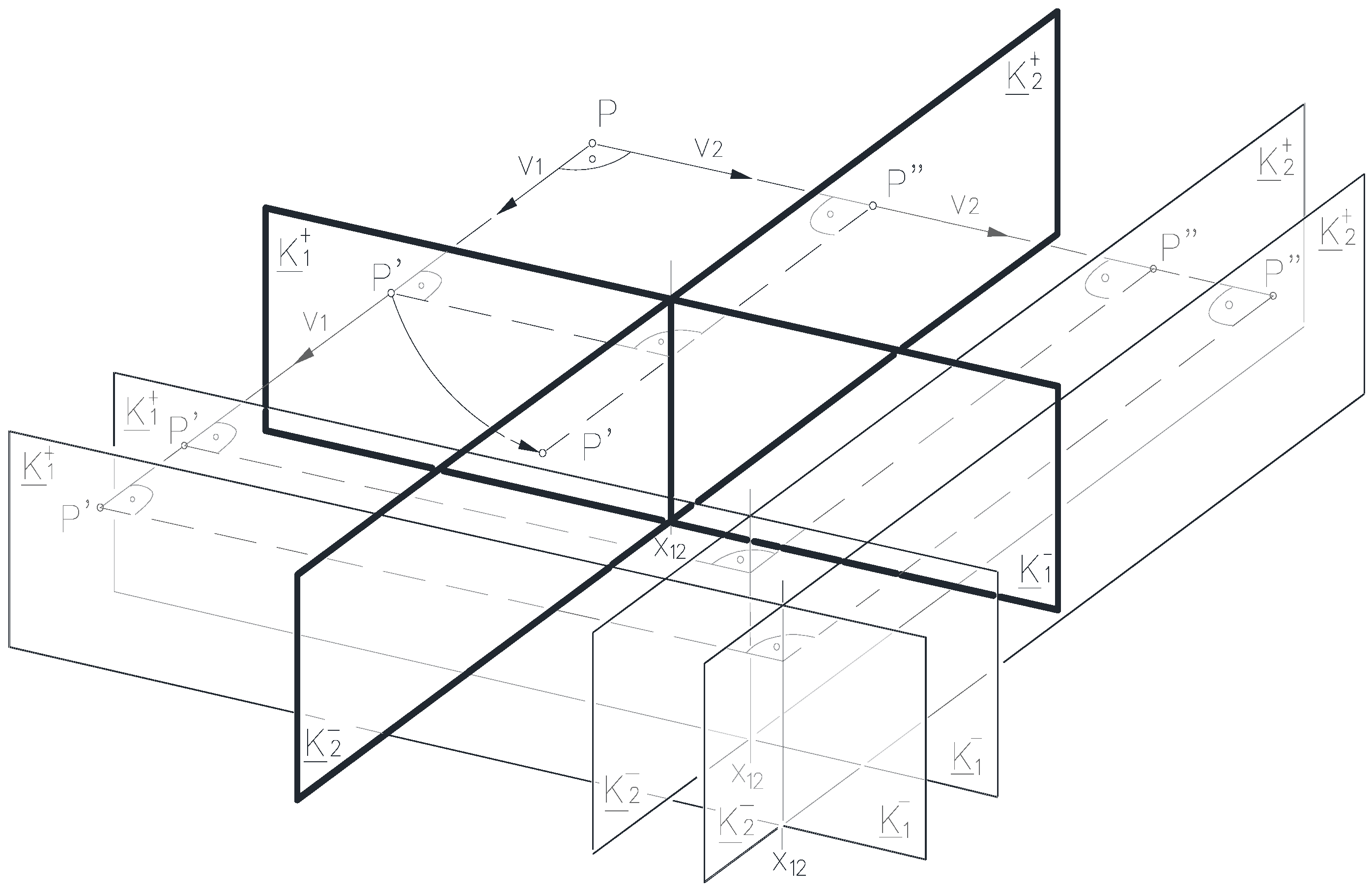
For a fixed curve of the space, the image plane system can be taken in an infinite number of ways. Among the Monge projections that can be added to a fixed curve of the space, there may be those in which the representation of any part of the curve is bijective, and other in which the representation of part of the curve is not bijective.

Theorem 5. 

Regarding a spatial object, the same result is obtained during the reconstruction procedure in all Monge projections that can be moved into each other by parallel displacement.

Proof of Theorem 5. 

Since the parallel translation is a congruence transformation, the translation does not change the image curves. □

Figure 5 shows some Monge projections that can be transformed into each other by parallel displacement.

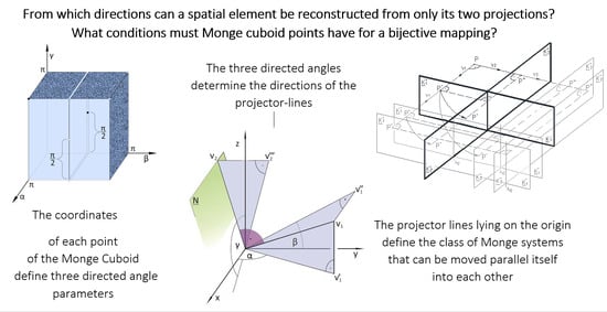
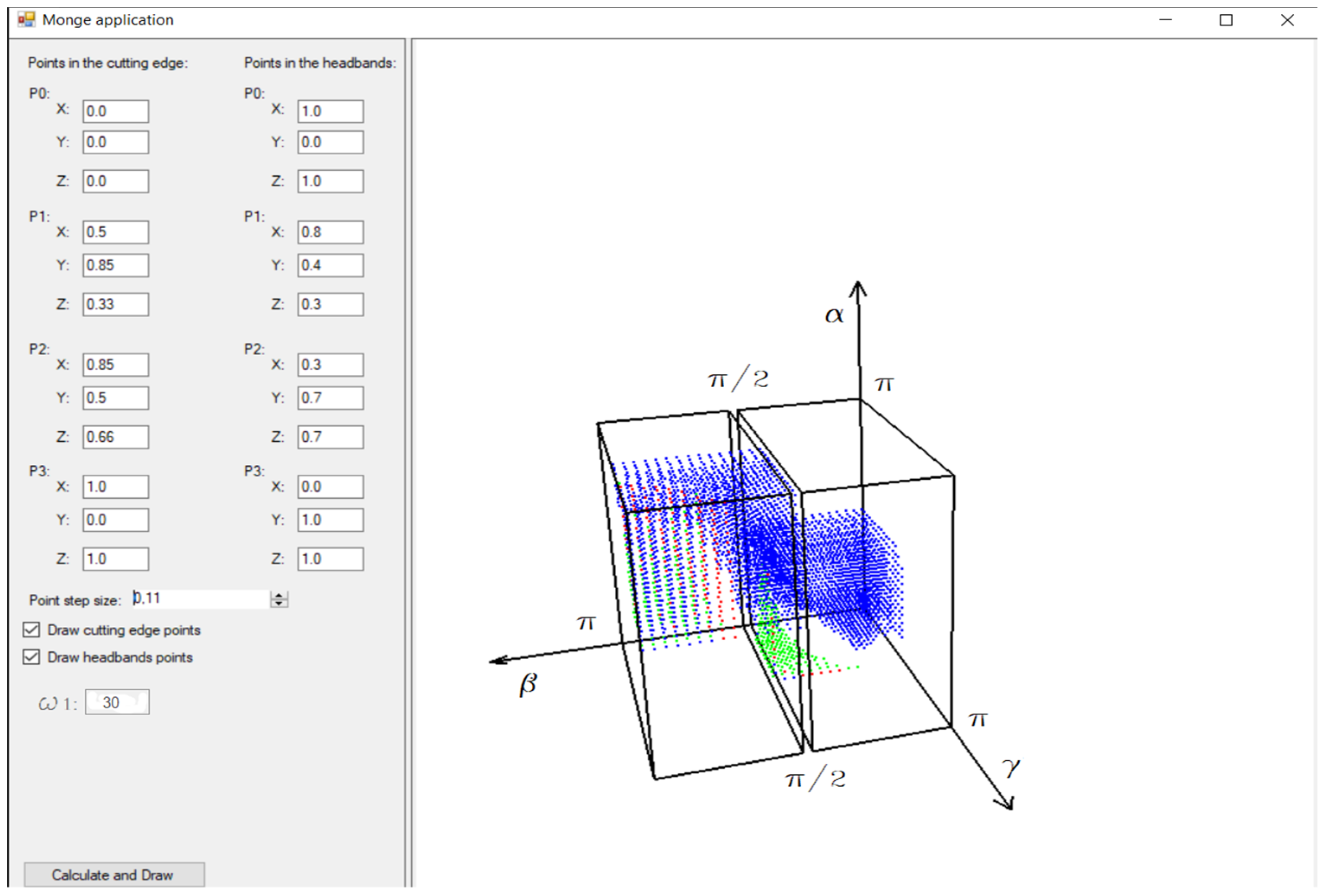
Therefore, in what follows, two Monge projections will be considered identical if their reference systems, namely their image plane systems can be moved into each other by parallel displacement. Based on the above, in order to facilitate the further investigations, a point O is fixed in the space, and it is expected that the image planes and projector lines of the Monge projections fit to this point. While the x₁₂ axis, namely the intersection line of the two image planes can be characterized by 2 free parameters, for example two spherical coordinates, the image planes can be described by 1 free parameter in the possibilities of rotation around the x₁₂ axis. Consequently, Monge projections can be described with 3 free parameters in addition to the previous restrictions. After all this, a number triple has been assigned to each Monge projection, with its elements having the geometric meaning of an angle. However, before assigning these, it is necessary to define the directed angles of the straight line.

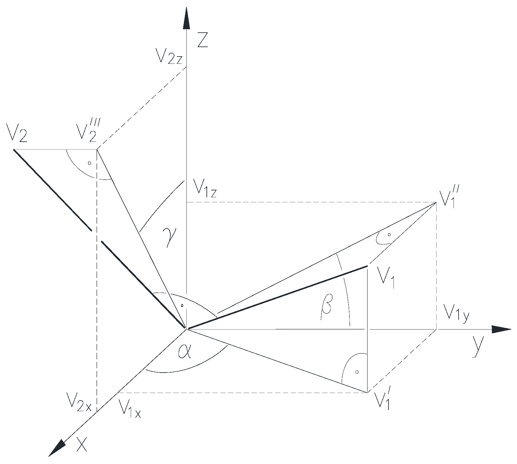
2.2.1. Directed Angles of the Straight Line

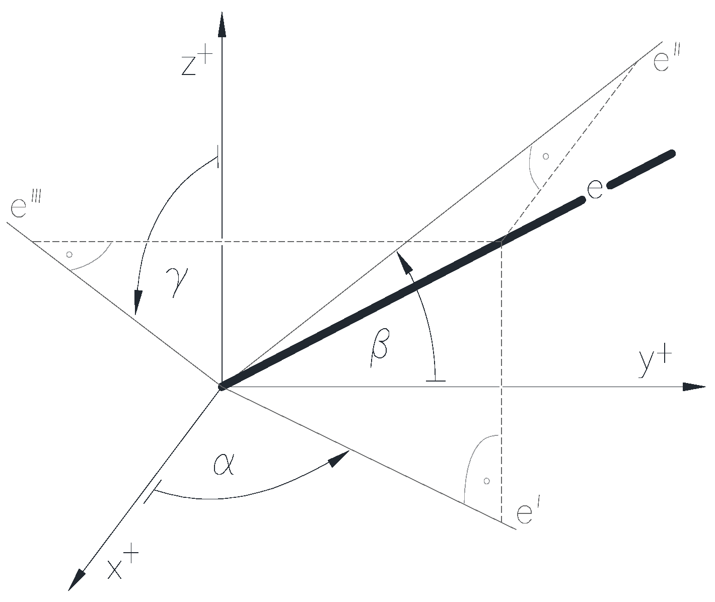
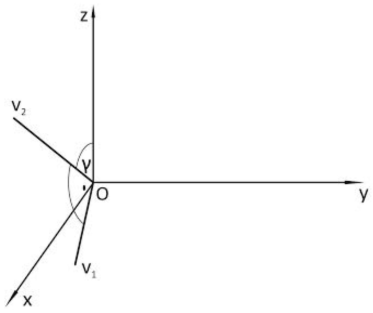
In order to create the definitions, an O[x, y, z] Cartesian coordinate system has to be fixed in the space. Directed angles of the straight line have been determined in this space fixed Cartesian coordinate system.

Definition 2. 

The first directed angle α (0 ≤ α ≤ π) of the straight line e passing through the origin point O is the angle, by which the semi-axis x⁺ can be rotated towards its first projection e′ of the straight line e on the plane [xy] in the direction of the semi-axis y⁺, counter- clockwise as viewed from a point at infinity on the semi-axis z⁺ (Figure 6). The first directed angle should be α = 0, if the straight line e coincides with the axis z. The first directed angle of the straight line bypassing the origin point O is the same as that of the one running parallel to it and passing through the origin point O.

Definition 3. 

The second directed angle β (0 ≤ β ≤ π) of the straight line e passing through the origin point O is the angle, by which the semi-axis y⁺ can be rotated to its second projection e″ of the straight line e on the plane [yz] in the direction of the semi-axis z⁺, counter- clockwise viewed from a point at infinity on the semi-axis x⁺ (Figure 6). The second directed angle should be β = 0, if the straight line e coincides with the axis x. The second directed angle of the straight line e bypassing the origin point O is the same as that of the one running parallel to it and passing through the origin O.

Definition 4. 

The third directed angle γ (0 ≤ γ ≤ π) of the straight line e passing through the origin point O is the angle by which the semi-axis z⁺ can be rotated to the third projection e‴ of the straight line e on the plane [zx] in the direction of the semi-axis x^+, counter-clockwise viewed from the infinity point of the semi-axis y⁺ (Figure 6). The third directed angle should be interpreted according to γ = 0, if the straight line e coincides with the axis y. The third directed angle of the straight line e bypassing the origin point O is the same as the third directed angle of the straight line parallel to it passing through the origin point O.

Theorem 6. 

If the image planes of the image planes system {K₁, K₂} of a Monge projection fit to a fix point O of the space, then the Monge projection is defined by its projector lines v₁ and v₂ passing through the origin O.

Proof of Theorem 6. 

The image planes K₁ and K₂ will be perpendicular v₁, and v_2, respectively. There are an infinite number of these pairs of planes, but the Monge systems are derived from each other with a parallel display, namely these are equivalent from the point of view of the present examination. □

Theorem 7. 

If a given Monge projection is bijective or nonbijective with respect to a given curve g, then the Monge projection obtained by exchanging the image planes K₁, K₂ and projector lines v₁, v₂ is also bijective or nonbijective with respect to the given curve g.

Proof of Theorem 7. 

By exchanging the image planes K₁ and K₂ and the projector lines v₁, v₂ the image curves g′ and g″ of the g curve do not modify, only their comma notations are exchanged, namely g′ becomes g″ and g″ becomes g′ because of the symmetry property. □

The goal is to create a mapping between the Monge projections and the number triplets that clearly characterize them, using the real directed angles defined above, in such a way that all ordered two-images must be discussed.

2.2.2. The Relationship between the Triplets of Directed Angles and the Monge Projections

Figure 5 shows some Monge projections that can be transformed into each other by parallel displacement.

Theorem 8. 

In addition to those Monge projections, whose projector lines v₁ and v₂ fulfil both the v₁ ∊ [zx] and v₂ ∉ [zx] conditions, define three independent parameters (α, β, γ) in a space fixed Cartesian coordinate system O[x, y, z] as follows: the first directed angle of the first projector line v₁ of the Monge projection should be parameter α, while the second directed angle should be parameter β, and the third directed angle of the second projector line v₂ should be parameter γ.

Figure 5 shows some Monge projections that can be transformed into each other by parallel displacement.

Remark 1. 

The mapping between the Monge projections satisfying the condition given in the Theorem 8 and the directed angles in the range 0 ≤ α, β, γ ≤ π is injective, but not surjective.

Proof of Theorem 8. 

The proof is divided into two parts: 1, when v₁ ∉ [zx], and 2, when v₁,v₂ ∈ [zx].

• The first projector line v₁ is not on the coordinate plane [zx] of the O[x, y, z] Cartesian coordinate system. The rotation of x⁺ on the plane [xy] by α into the direction of y⁺ yields the first image v₁′ of the projector line v₁, to which the plane V₁ fits and is perpendicular to the plane [xy]. Then, the rotation of y⁺ on the plane [yz] by into the direction of z⁺ results the second image v₁″ of the projector line v₁, to which the plane V₂ fits and is perpendicular to the plane [yz]. Since the assumption v₁∉ [zx] is hold, there exists a straight line of intersection of planes V₁ and V₂, serving as the first projector line v₁ of the sought Monge projection. Then, the rotation of z⁺ on the plane [zx] with γ into the direction of x⁺ yields the third image v₂‴ of the projector line v₂, to which the plane V₃ fits and is perpendicular to the plane [zx]. Again, due to our assumption v₁ ∉ [zx], the plane N perpendicular to v₁ can never coincides with plane V₃, so there is a straight line of intersection of planes N and V₃. This is the second projector line v₂ of the Monge projection (Figure 7).
  Based on Theorem 6, the projector lines v₁ and v₂ determine the Monge projection.
• The first and second projector lines v₁ and v₂ fit on the coordinate plane [zx] of the Cartesian coordinate system O[x, y, z]. In this case, the corresponding Monge projection is derived from the directed angles triplet (α, β, γ) by rotating z⁺ in the direction of x⁺ by γ on the plane [zx]. This will be the second projector line v₂ of the sought Monge projection, and then the first projector line of v₁ is perpendicular to it as shown in Figure 8. □

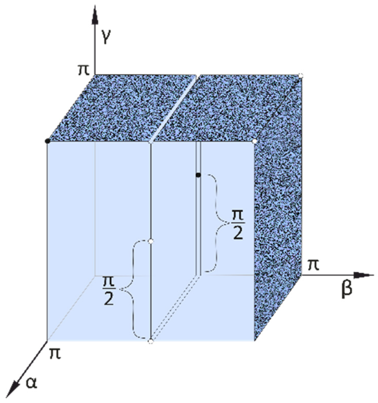
It must also be stated here that based on Theorem 6, the projector lines v₁ and v₂ determines the Monge projection. Since v₁ has a first and a second directed angle and v₂ has a third directed angle by definition, each Monge projection can be assigned one number triple only. According to the reverse assignment, each point of the Monge cuboid defines a triplet of real numbers, the geometric meaning of which is a directed angle, which provides a Monge projection respected to the given curve.

Definition 5. 

In the O[α, β, γ] Cartesian coordinate system, the subset of the elements of the directed angle triples (α, β, γ) within the range [0, π] to which a Monge projection clearly belongs is called a Monge cuboid.

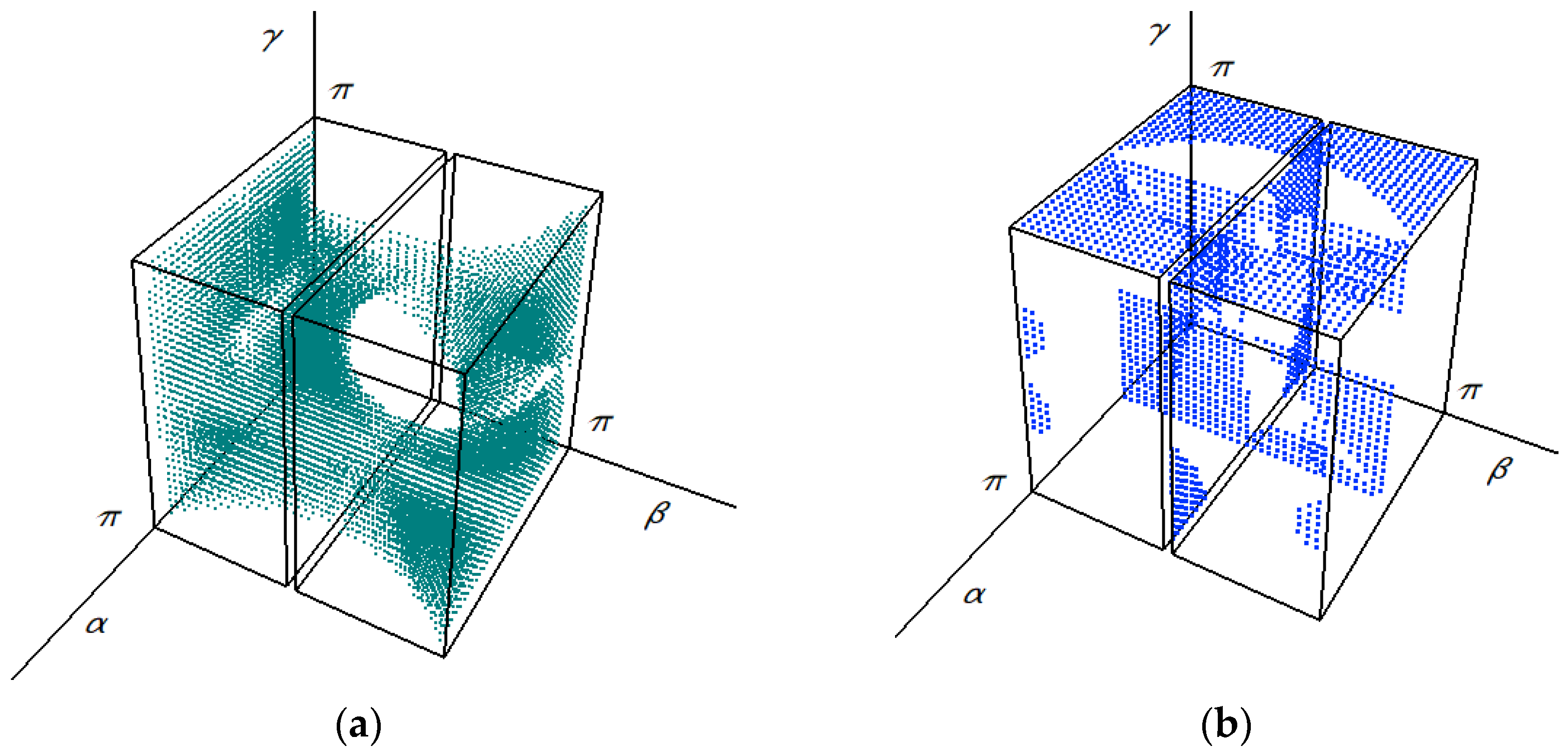
After examining which are the triplets satisfying the conditions 0 ≤ α, β, γ ≤ π that cannot be assigned to a Monge projection, due to the statements made previously, the points of the π × π × π cube that do not belong to the Monge projection to the Monge cuboid can also be determined.

The points satisfying the following condition are located inside the Monge cuboid as illustrated by Figure 9.

$$\begin{array}{ccccc} 0 < \alpha < \pi ,& 0 < \beta < \pi /2& \mathrm{and}& \pi /2 < \beta < \pi ,& 0 < \gamma < \pi \end{array}$$

(1)

Points satisfying the following conditions are located on the surface of the Monge cuboid as illustrated by Figure 9.

$$\left.\begin{array}{l}\begin{array}{llll}-& 0<\alpha <\pi ,& \beta =\pi ,& 0<\gamma <\pi \end{array}\\ \begin{array}{lllll}-& 0<\alpha <\pi ,& 0<\beta <\pi /2 \mathrm{and}& \pi /2<\beta <\pi ,& \gamma =\pi \end{array}\\ \begin{array}{lllll}-& \alpha =\pi ,& \beta =\pi /2,& 0<\gamma <\pi /2 \mathrm{and}& \pi /2<\gamma <\pi \end{array}\\ \begin{array}{llll}-& \alpha =0,& \beta =\pi /2,& \gamma =\pi /2\end{array}\\ \begin{array}{llll}-& \alpha =\pi ,& \beta =0,& \gamma =\pi \end{array}\end{array}\right\}$$

(2)

In summary, according to the presented procedure, a Monge projection is assigned to a point of the Monge cuboid by interpreting the triplet of angle parameters as coordinates. Inversely, any point of the Monge cuboid defines a Monge projection by interpreting its coordinates as a triplet of directed angles. A mathematical mapping is created between Monge projections and Monge cuboid points. This method covers all two orthogonal projections assigned to each other that are relevant in engineering due to their symmetry property due to their interchangeability. This is suitable for carrying out our analyses, because the test of reconstructability with respect to a curve results in the same conclusion by exchanging the first and second views. The presentation of the method was based on what was described in the literature [49].

2.3. Application of the Method

When applying the method, there are 3 important points to consider:

• The curve must be positioned in a fixed O[x, y, z] initial Cartesian coordinate system.
• The direction cone formed from the directions of the tangents of the curve must be determined, that is, the tangents of the curve must be moved parallel to themselves into a properly selected point of the z axis, such as the origin O, by parallel displacement.
• Examining the mutual positions of the profile planes of the Monge projections and the directional cone, it is necessary to find the cases when they do not have a common line.

The correctness of the method can be immediately checked and verified by the practitioners of descriptive geometry through the examples presented below.

2.3.1. Procedure for Representing a Straight Line

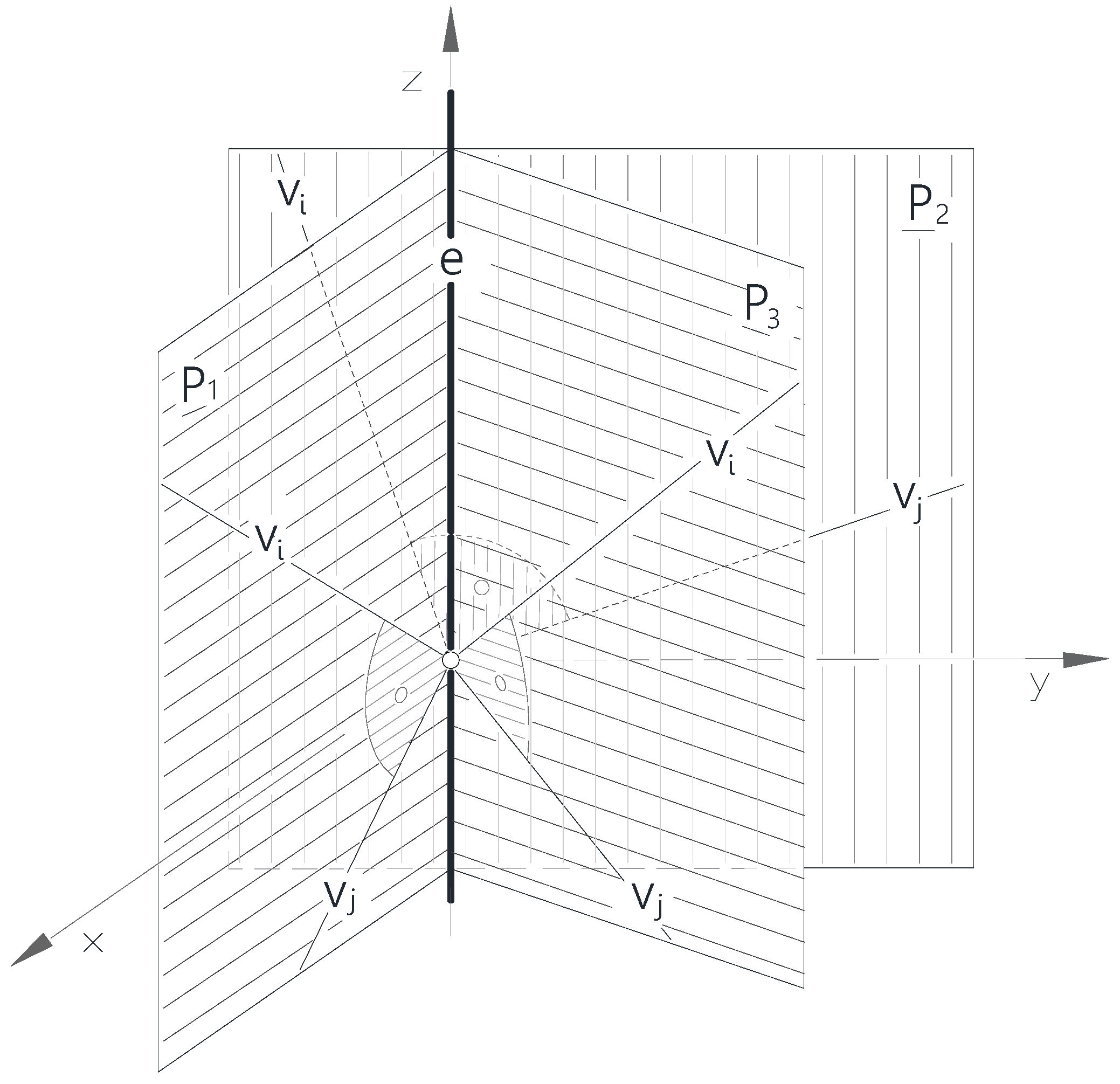
It is advisable to choose the mutual position of the straight line and the Cartesian coordinate system as simply as possible. Therefore, it is convenient to define line e as one coinciding with one of the coordinate axes, such as the z, as shown in Figure 10.

In this case, the direction cone of the straight line e is formed by the tangents moved to the point O characterized by coordinates (0, 0, 0), namely the axis z itself. Consequently, in any Monge projection, it is not possible to reconstruct the line e from only its two images, in which the profile plane P of the Monge projection also fits the axis z, namely P is an element of the planes series fitting on the axis z, unless the straight line e is a projector line. In the case of the representation of the line e coinciding with coordinate axis z, the nonbijective subset of the Monge cuboid can be determined in three position of the profile plane, which are explained in the following:

• In the first case, the profile plane labeled P₁ fits on the [zx] coordinate plane, namely P₁ ≡ [zx], as well as the projector lines v₁ and v₂ do not fit on either the z or x coordinate axes. In this case, the subset to be found is declared by angle triples satisfying the following conditions

$$\begin{array}{ccccc}\alpha =\pi ,& \beta =\pi /2,& 0 < \gamma < \pi /2& \mathrm{and}& \pi /2 <\gamma < \pi \end{array}$$

(3)

2.

In the second case, the profile plane labeled P2 fits on the [yz] coordinate plane, namely P2 ≡ [yz], as well as the projector lines v1 and v2 do not fit on either the y or x coordinate axes. In this case, the subset to be found is declared by angle triples satisfying the following conditions

$$\begin{array}{ccccc} \alpha =\pi /2,& 0 < \beta <\pi /2& \mathrm{and}& \pi /2< \beta < \pi ,& \gamma =\pi \end{array}$$

(4)

3.

In the third case, as outlined in Figure 10, the profile plane in position P₃ contains on the z coordinate axis, but does not contain either of the x or y coordinate axes, and none of the projector lines lie onto the z coordinate axis.

In this case, the first directed angle value can be chosen according to the conditions 0 < α < π/2 and π/2 < α < π. In the case of a fix α value, the second directed angle can be chosen according to the conditions 0 < β < π/2 and π/2 < β < π. In the case of a fixed α and β, what conditions γ fulfills was investigated.

To examine the projector lines lying the profile plane P₃ the direction vector of the first projector line v₁ should be v₁(v_1x, v_1y, v_1z), the direction vector of the second projection line v₂ should be v₂(v_2x, v_2y, v_2z) as shown in Figure 11.

In the case of P₃, the n normal vector of the first projector plane V₁ lying to the v₁ and v₂ projector lines should be n = (v_1y, −v_1x, 0).

Since v₂⊥v₁ and v₂⊥n, due to the following relation

$$v_2=v_1\times n$$

(5)

the coordinates of the v₂ second projector line are

$$\left({\mathrm{v}}_{1\mathrm{x}}\cdot {\mathrm{v}}_{1\mathrm{z} }{, \mathrm{v}}_{1\mathrm{y}}\cdot {\mathrm{v}}_{1\mathrm{z} }, -{\mathrm{v}}_{1\mathrm{x}}^2-{\mathrm{v}}_{1\mathrm{y}}^2\right)$$

(6)

As can be seen in Figure 11, in the case of conditions α, β, γ ≠ 0, π, relation

$${\cos }^2\mathsf{\alpha }={\mathrm{v}}_{1\mathrm{x}}^2/\left({\mathrm{v}}_{1 \mathrm{x}}^2+{\mathrm{v}}_{1\mathrm{y}}^2\right)$$

(7)

and based on Figure 11, under the α, β, γ ≠ 0, π conditions, the following simple relationships can be established

$$\left.\begin{array}{c}\mathrm{tg}\mathsf{\alpha }={ \mathrm{v}}_{1\mathrm{y}}/{\mathrm{v}}_{1\mathrm{x}}\\ \mathrm{tg}\mathsf{\beta }={ \mathrm{v}}_{1\mathrm{z}}/{\mathrm{v}}_{1\mathrm{y}}\\ \mathrm{tg}\mathsf{\gamma }={ \mathrm{v}}_{2\mathrm{x}}/{\mathrm{v}}_{2\mathrm{z}}\end{array}\right\}$$

(8)

and the α, β, γ ≠ π/2 exclusions, the following conclusions can be drawn

$$\left.\begin{array}{c}\mathrm{ctg}\mathsf{\alpha }={ \mathrm{v}}_{1\mathrm{x}}/{\mathrm{v}}_{1\mathrm{y}}\\ \mathrm{ctg}\mathsf{\beta }={ \mathrm{v}}_{1\mathrm{y}}/{\mathrm{v}}_{1\mathrm{z}}\\ \mathrm{ctg}\mathsf{\gamma }={ \mathrm{v}}_{2\mathrm{z}}/{\mathrm{v}}_{2\mathrm{y}}\end{array}\right\}$$

(9)

Based on the known trigonometric relations presented in (8) and (9), the following equation can be obtained for a fixed pair of (α, β)

$$\mathsf{\gamma }=\mathrm{arctg}\left(-\cos \mathsf{\alpha }\cdot \sin \mathsf{\alpha }\cdot \mathrm{tg}\mathsf{\beta }\right)$$

(10)

Coordinates of the points belonging to the nonbijective subset of the Monge cuboid fulfill the following conditions in the case of the straight line e lying on the z coordinate axis

$$\left.\begin{array}{l}\begin{array}{llll}- \mathsf{\alpha }=\mathsf{\pi },& \mathsf{\beta }=\mathsf{\pi }/2,& 0 < \mathsf{\gamma } < \mathsf{\pi }/2& \mathrm{and} \mathsf{\pi }/2 < \mathsf{\gamma } < \mathsf{\pi }\end{array}\\ \begin{array}{llll}- \mathsf{\alpha }=\mathsf{\pi }/2, & 0 < \mathsf{\beta } <\mathsf{\pi }/2 \mathrm{and}& \mathsf{\pi }/2< \mathsf{\beta } < \mathsf{\pi },& \mathsf{\gamma }=\mathsf{\pi }\end{array}\\ \begin{array}{lll}- 0 < \mathsf{\alpha }, \mathsf{\beta } <\mathsf{\pi }/2& \mathrm{and} \mathsf{\pi }/2 < \mathsf{\alpha }, \mathsf{\beta } < \mathsf{\pi },& \mathsf{\gamma }\ne 0\end{array}\Rightarrow \gamma =\mathrm{arctg}\left(-\cos \mathsf{\alpha }\cdot \sin \mathsf{\alpha }\cdot \mathrm{tg}\mathsf{\beta }\right)\end{array}\right\}$$

(11)

2.3.2. Procedure for Representing a Circle

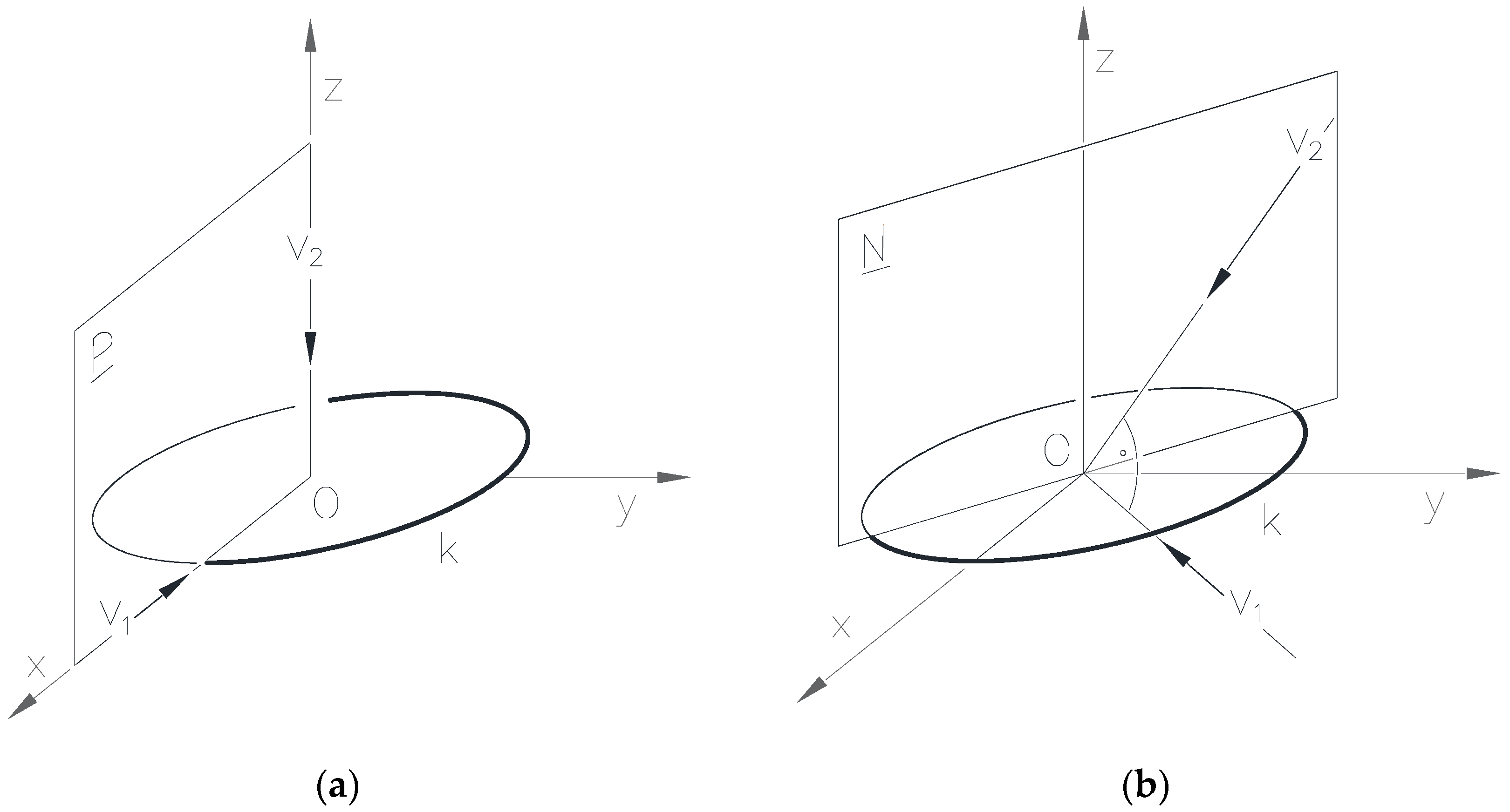
The examination has been carried out in the case of a circle on the [xy] plane with its center in the origin of the Cartesian coordinate system. In this case, by shifting the tangents of the circle to the origin point O, the special cone of the tangent directions is a series of straight lines in a radial position on the [xy] plane with the origin O as the center. The direction cone of the circle is intersected by the profile plane of every Monge projection passing through the origin, that is, the circle has a tangent in the profile direction. It should be noted that if the profile plane coincides with the plane [xy], the two images of the circle are each a diameter-length section. If the first projector line v₁ or the second projector line v₂ lies in the plane [xy], then one of the images of the circle is a diameter-length section, namely a double projection, so it can be described as a function on the corresponding Cartesian coordinate plane, while the other image is a circle or an ellipse. In this exceptional case, the representation of the circle with the given location is bijective. For the reasons listed earlier, there are two cases to be considered:

• If the v₁ ∈ [xy] and v₂ ∉ [xy] are fulfilled, the representation of the given circle is bijective. For v₁ ∉ x, see Figure 12a). For v₁∈x and v₂∈z, see Figure 12b).

2.

Where v₂ ∈ [xy] and v₁ ∉ [xy], the fulfillment of the v₁∈z condition is determined by the directed angles α = 0, β = π/2 and γ = π/2 as shown in Figure 13a), so the circle can be clearly represented. If v₂ ∈ [xy] and v₁ ∉ [xy] are fulfilled as shown in Figure 13b), the representation of the given circle is bijective.

Based on the reasoning, the triplets of directed angles that meet the following conditions are interpreted as coordinates and such as result the points of the bijective part of the Monge cuboid with respect to the circle placed in the determined position

$$\left.\begin{array}{l}\begin{array}{llll}- 0 < \mathsf{\alpha } < \mathsf{\pi },& \mathsf{\beta }=\mathsf{\pi },& 0 < \mathsf{\gamma } < \mathsf{\pi }/2& \mathrm{and} \mathsf{\pi }/2 <\mathsf{\gamma } < \mathsf{\pi }\end{array}\\ \begin{array}{lll}- \mathsf{\alpha }=\mathsf{\pi },& \mathsf{\beta }=0, & \mathsf{\gamma }=\mathsf{\pi }\end{array}\\ \begin{array}{llll}- 0 < \mathsf{\alpha } < \mathsf{\pi },& 0 < \mathsf{\beta } <\mathsf{\pi }/2 \mathrm{and}& \mathsf{\pi }/2< \mathsf{\beta } < \mathsf{\pi },& \mathsf{\gamma }=\mathsf{\pi }/2\end{array}\\ \begin{array}{lll}- \mathsf{\alpha }=0,& \mathsf{\beta }=\mathsf{\pi }/2,& \mathsf{\gamma }=\mathsf{\pi }/2\end{array}\end{array}\right\}$$

(12)

The three free parameters represented by the directed angle parameters satisfying the above conditions define suitable directions for locating the two CCD cameras, so that the circle can be reconstructed from the two images taken by them.

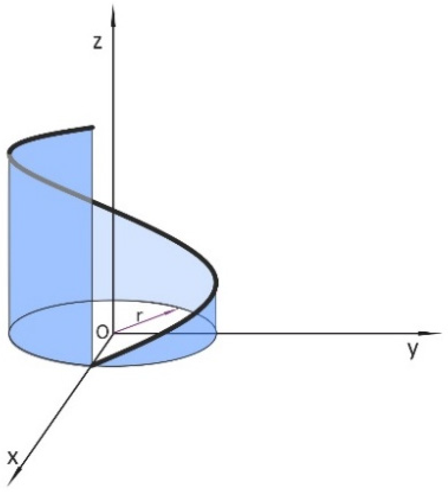
2.3.3. Procedure for Representing a Helix

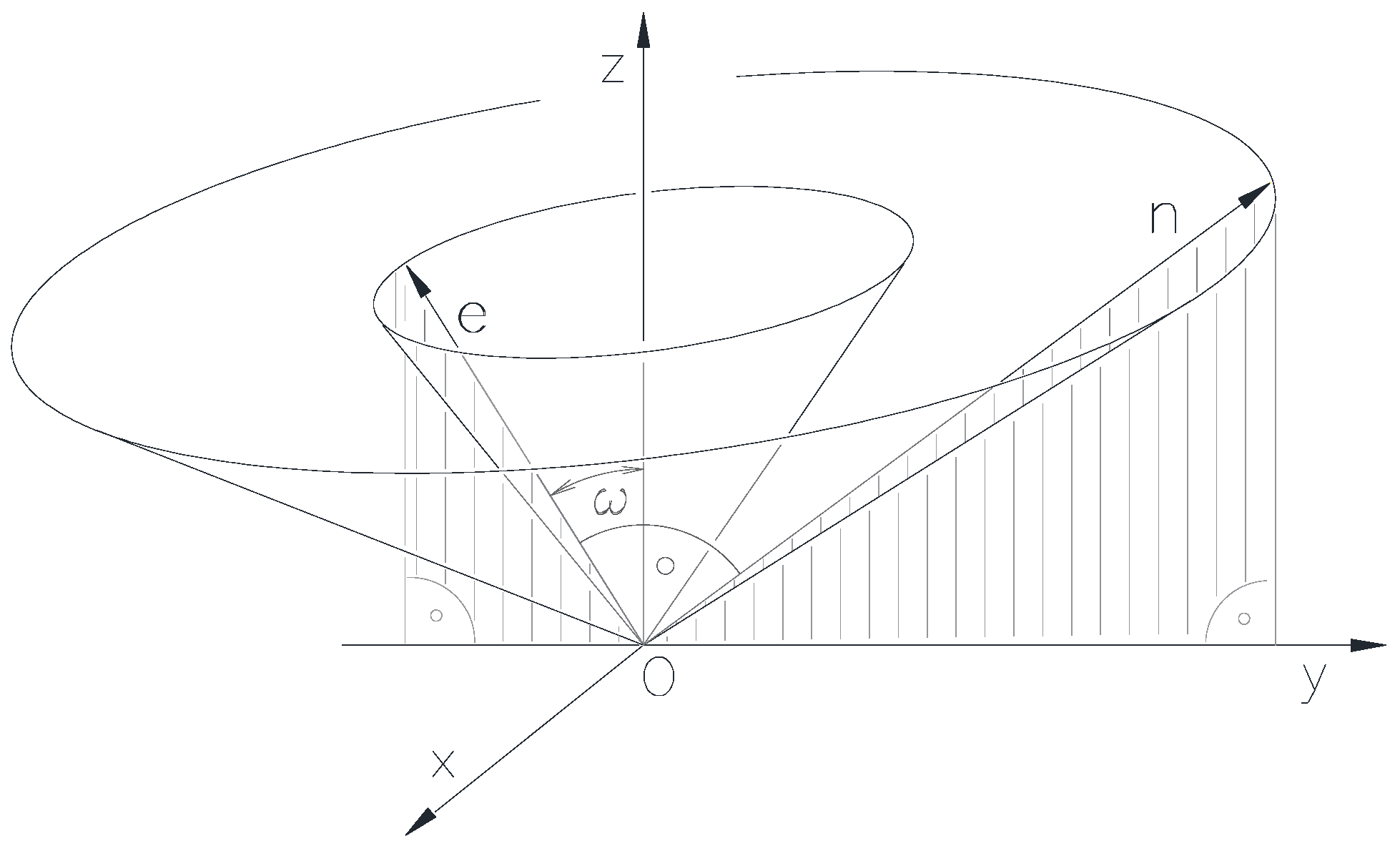
The center line of the helix should practically coincide with the z coordinate axis of the Cartesian coordinate system, as shown in Figure 14.

Because of the cyclicity of the curve, the helix has been examined for one thread pitch. The parametric equation of one thread of the helix with the thread pitch parameter p on a cylinder with radius r and axis z is

$$\left.\begin{array}{l}x=r\cdot \cos \phi \\ y=r\cdot \sin \phi \\ z=p\cdot \phi \end{array}\right\}$$

(13)

where p ∊ ℝ \{0}, r ∊ ℝ⁺, 0 ≤ φ < 2π.

The derivate coordinates of the helix result in the tangent vectors r_e

$$\left.\begin{array}{l}{\mathrm{x}}_{\mathrm{e}}=r\cdot \sin \mathsf{\phi }\\ {\mathrm{y}}_{\mathrm{e}}=-r\cdot cos\phi \\ {\mathrm{z}}_{\mathrm{e}}=p\end{array}\right\}$$

(14)

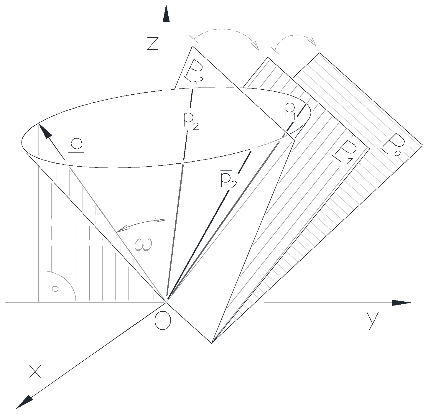
The direction cone of the helix is created by the tangents moved parallel to themselves to the origin point O. The half opening angle of the direction cone of the tangent vectors is the constant angle ω. In any Monge projection, whose profile plane P₂ contains two generatrixes of the direction cone of the tangents as shown in Figure 15, the representation of a pitch of the helix results two tangents in profile direction.

This means that there is a part of the helix whose representation is not clear, namely it is not bijective in the Monge projection belonging to the profile plane at position P₂.

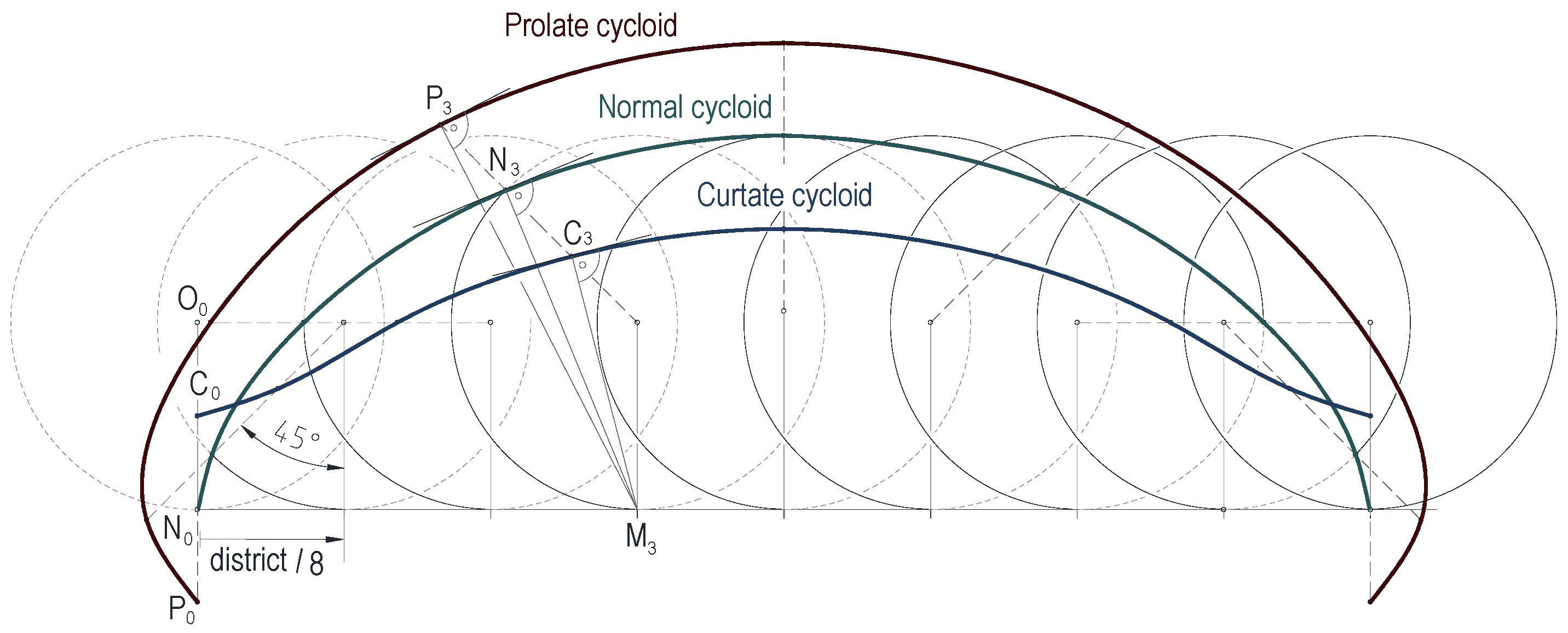
If the profile plane of a Monge projection contains one tangent straight line of the cone of tangents to one thread of the helix, as that can be seen in the profile plane at position P₁ in Figure 15, then at the point belonging to the profile-oriented tangent straight line of the helix, the tangent straight line intersects the image curves, namely this point is the singular points of the image curves, due to the cyclicity of the helix and its images. In this case, any part of the helix can be clearly reconstructed from its two images. If the cone of the tangential directions of the helix does not have a single common straight line with the profile plane of the Monge projection, namely the profile plane in position P₀ as shown in Figure 15. In this case, the images of the helix are curtate cycloids (Figure 16) or planar curves, which are in affine relationship to the curtate cycloids and contain inflection points. In the case of such a Monge projection, any segment of the helix can be unambiguously reproduced from its first and second images.

The normal vectors n(n_x, n_y, n_z) are perpendicular to the tangent planes of the cone of tangent directions of the helix. The normal vectors placed at the origin O create the normal cone, as shown in Figure 17.

The generatrixes of the normal cone of the helix are the normal of the tangent planes of the tangent cone. Let us take the direction vector of the normal cone generatrix n. Let us have the vector n(n_x, n_y, n_z) as the unit vector, namely |n| = 1, and z(0, 0, 1) defined as one coinciding with the axis z.

The scalar product of the unit vectors

$$n\cdot z=\left|n\right|\cdot \left|z\right|\cdot \cos \left(90°-\mathsf{\omega }\right)=\sin \mathsf{\omega }$$

(15)

and

$$n\cdot z={\mathrm{n}}_{\mathrm{x}}\cdot 0+{\mathrm{n}}_{\mathrm{y}}\cdot 0+{\mathrm{n}}_{\mathrm{z}}\cdot 1$$

(16)

so

$${ \mathrm{n}}_{\mathrm{z}}=\sin \mathsf{\omega }$$

(17)

Due to the condition $\left|n\right|=1$.

$${\mathrm{n}}_{\mathrm{x}}^2+{\mathrm{n}}_{\mathrm{y}}^2+{\mathrm{n}}_{\mathrm{z}}^2=1$$

(18)

Substituting the result of Equation (17) into Equation (18) yields the equation

$${\mathrm{n}}_{\mathrm{x}}^2+{\mathrm{n}}_{\mathrm{y}}^2+{\sin }^2\mathsf{\omega }=1$$

(19)

which may be converted into the following form

$${\mathrm{n}}_{\mathrm{x}}^2+{\mathrm{n}}_{\mathrm{y}}^2={\cos }^2\mathsf{\omega }$$

(20)

Equation (18) is the equation of a circle with a radius of cosω.

It can be established that the tangent direction cone of the stated helix and the profile plane P of a Monge projection, in event that the condition is fulfilled

$${\mathrm{n}}_{\mathrm{x}}^2+{ \mathrm{n}}_{\mathrm{y}}^{2 }{> \cos }^2\mathsf{\omega }$$

(21)

will have two common cone generatrixes, while in case of

$${\mathrm{n}}_{\mathrm{x}}^2+{ \mathrm{n}}_{\mathrm{y}}^2={\cos }^2\mathsf{\omega }$$

(22)

will have one common cone generatrix. If

$${\mathrm{n}}_{\mathrm{x}}^2+{ \mathrm{n}}_{\mathrm{y}}^2{ < \cos }^2\mathsf{\omega }$$

(23)

no common cone generatrix is present.

The aim is to determine the n(n_x, n_y, sinω) normal vectors satisfying relations (22) and (23), and to provide the coordinates α, β, γ of the points of the Monge cuboid that define bijective Monge projections for the given helix. Profile planes perpendicularly to the normal vectors, then the Monge projections belonging to the profile planes, and finally to specify some conditions of the relations between the α, β, γ coordinates of the points of the Monge cuboid.

In summary, the goal is to provide the coordinates α, β, γ of the points of the Monge cuboid that define bijective Monge projections for the given helix.

Since the projector lines v₁ and v₂ are perpendicular to each other, so their direction vectors v₁ and v₂ are also perpendicular to each other, as a result of which the following relation is fulfilled

$$v_1\cdot v_2=0$$

(24)

The relation (24) can be converted into the following forms using the coordinates of the direction vectors v₁(v_1x, v_1y, v_1z) and v₂(v_2x, v_2y, v_2z)

$${\mathrm{v}}_{1\mathrm{x}}\cdot {\mathrm{v}}_{2\mathrm{x}}+{ \mathrm{v}}_{1\mathrm{y}}\cdot {\mathrm{v}}_{2\mathrm{y}}+{\mathrm{v}}_{1\mathrm{z}}\cdot {\mathrm{v}}_{2\mathrm{z}}=0$$

(25)

This may be further converted as

$${\mathrm{v}}_{2\mathrm{y}}=-\left({\mathrm{v}}_{1\mathrm{x}}\cdot {\mathrm{v}}_{2\mathrm{x}}+{\mathrm{v}}_{1\mathrm{z}}\cdot {\mathrm{v}}_{2\mathrm{z}}\right)/{\mathrm{v}}_{1\mathrm{y}}$$

(26)

I.

In the first part of the examination, the assumptions α,β,γ ≠ 0,π/2,π are considered.

It is known that

$$n=v_1\times v_2$$

(27)

which can be written in the following forms

$${\mathrm{n}}_{\mathrm{x}}={\mathrm{v}}_{1\mathrm{y}}\cdot {\mathrm{v}}_{2\mathrm{z}}-{\mathrm{v}}_{2\mathrm{y}}\cdot {\mathrm{v}}_{1\mathrm{z}}$$

(28)

and based on Equations (8) and (9)

$${\mathrm{n}}_{\mathrm{x}}=\left(\mathrm{ctg}\mathsf{\beta }+\mathrm{ctg}\mathsf{\alpha }\cdot \mathrm{tg}\mathsf{\gamma }+\mathrm{tg}\mathsf{\beta }\right)\cdot {\mathrm{v}}_{1\mathrm{z}}\cdot {\mathrm{v}}_{2\mathrm{z}}$$

(29)

as well as

$${\mathrm{n}}_{\mathrm{y}}={\mathrm{v}}_{1\mathrm{z}}\cdot {\mathrm{v}}_{2\mathrm{x}}-{ \mathrm{v}}_{2\mathrm{z}}\cdot {\mathrm{v}}_{1\mathrm{x}}$$

(30)

and based on Equations (8) and (9)

$${\mathrm{n}}_{\mathrm{y}}=\left(\mathrm{tg}\mathsf{\gamma }-\mathrm{ctg}\mathsf{\beta }\cdot \mathrm{ctg}\mathsf{\alpha }\right)\cdot {\mathrm{v}}_{1\mathrm{z}}\cdot {\mathrm{v}}_{2\mathrm{z}}$$

(31)

furthermore

$${\mathrm{n}}_{\mathrm{z}}={\mathrm{v}}_{1\mathrm{x}}\cdot {\mathrm{v}}_{2\mathrm{y}}-{\mathrm{v}}_{2\mathrm{x}}\cdot {\mathrm{v}}_{1\mathrm{y}}$$

(32)

and based on Equations (8) and (9)

$${\mathrm{n}}_{\mathrm{z}}=\left(- \mathrm{ctg}\mathsf{\alpha }-\mathrm{tg}\mathsf{\beta }\cdot \mathrm{ctg}\mathsf{\gamma }-\mathrm{tg}\mathsf{\alpha }\right)\cdot {\mathrm{v}}_{1\mathrm{x}}\cdot {\mathrm{v}}_{2\mathrm{x}}$$

(33)

Since 0 < ω < π/2, the equation n_z = sinω ≠ 0 is fulfilled. In this case, the substitution with the equations (9) and (28)–(33) gives

$${\mathrm{n}}_{\mathrm{x}}/{\mathrm{n}}_{\mathrm{z}}=\left(\mathrm{tg}\mathsf{\alpha }\cdot \mathrm{ctg}\mathsf{\gamma }+\mathrm{tg}\mathsf{\beta }+\mathrm{tg}\mathsf{\alpha }\cdot {\mathrm{tg}}^2\mathsf{\beta }\cdot \mathrm{ctg}\mathsf{\gamma }\right)/\left(-\mathrm{ctg}\mathsf{\alpha }-\mathrm{tg}\mathsf{\beta }\cdot \mathrm{ctg}\mathsf{\gamma }-\mathrm{tg}\mathsf{\alpha }\right)$$

(34)

as well as

$${\mathrm{n}}_{\mathrm{y}}/{\mathrm{n}}_{\mathrm{z}}=\left(\mathrm{tg}\mathsf{\alpha }\cdot \mathrm{tg}\mathsf{\beta }-\mathrm{ctg}\mathsf{\gamma }\right)/\left(-\mathrm{ctg}\mathsf{\alpha }-\mathrm{tg}\mathsf{\beta }\cdot \mathrm{ctg}\mathsf{\gamma }-\mathrm{tg}\mathsf{\alpha }\right)$$

(35)

Substitution with the equation n_z = sinω gives

$${\mathrm{n}}_{\mathrm{x}}=\sin \mathsf{\omega }\cdot \left(\mathrm{tg}\mathsf{\alpha }\cdot \mathrm{ctg}\mathsf{\gamma }+\mathrm{tg}\mathsf{\beta }+\mathrm{tg}\mathsf{\alpha }\cdot {\mathrm{tg}}^2\mathsf{\beta }\cdot \mathrm{ctg}\mathsf{\gamma }\right)/\left(-\mathrm{ctg}\mathsf{\alpha }-\mathrm{tg}\mathsf{\beta }\cdot \mathrm{ctg}\mathsf{\gamma }-\mathrm{tg}\mathsf{\alpha }\right)$$

(36)

as well as

$${\mathrm{n}}_{\mathrm{y}}=\sin \mathsf{\omega }\cdot \left(\mathrm{tg}\mathsf{\alpha }\cdot \mathrm{tg}\mathsf{\beta }-\mathrm{ctg}\mathsf{\gamma }\right)/\left(-\mathrm{ctg}\mathsf{\alpha }-\mathrm{tg}\mathsf{\beta }\cdot \mathrm{ctg}\mathsf{\gamma }-\mathrm{tg}\mathsf{\alpha }\right)$$

(37)

From the above, the following conclusions can be drawn based on the relationships (22) and (23):

If the tangents and the axis of a helix form an angle ω, then the triplets (α, β, γ) satisfying the relation

$$\begin{array}{c}{(\left({\mathrm{tg}\mathsf{\alpha }·\mathrm{ctg}\mathsf{\gamma }+\mathrm{tg}\mathsf{\beta }+\mathrm{tg}\mathsf{\alpha }·\mathrm{tg}}^2\mathsf{\beta }·\mathrm{ctg}\mathsf{\gamma }\right)/\left(-\mathrm{ctg}\mathsf{\alpha }-\mathrm{tg}\mathsf{\beta }·\mathrm{ctg}\mathsf{\gamma }-\mathrm{tg}\mathsf{\alpha }\right))}^2\\ +{(\left(\mathrm{tg}\mathsf{\alpha }\cdot \mathrm{tg}\mathsf{\beta }-\mathrm{ctg}\mathsf{\gamma }\right)/\left(- \mathrm{ctg}\mathsf{\alpha }-\mathrm{tg}\mathsf{\beta }·\mathrm{ctg}\mathsf{\gamma }-\mathrm{tg}\mathsf{\alpha }\right))}^2\le {\mathrm{ctg}}^2\mathsf{\omega }\end{array}$$

(38)

are the coordinates of the points belonging to the bijective subset of the Monge cuboid.

It should be noted that in the Monge projections defined by the triplets satisfying condition (38), the images of the helix will contain singular points.

If ω = π/4, the triplets α = π/6, β = π/6 and γ = π/3 fulfills the condition (38), so as shown in Figure 18, any section of the helix can be reconstructed from only two of its images.

Condition (38) is fulfilled for ω = π/4 and for the angular triplet α = π/4, β = π/4, γ = π/4. Since the left and right sides of condition (38) are equal in this case, the helix has a profile direction tangent intersecting of a complete course of it, so any section of it can be clearly reconstructed from its two images, as shown in Figure 19.

In the case of ω = π/4, the triplet α = π/3, β = π/4, γ = 2·π/3 does not fulfill the condition (38), so in the Monge projection belonging to these directed angles there are parts of a complete run of the helix that cannot be clearly reconstructed based on their two images only, without any additional information (Figure 20).

Note that when the angles formed by the projection lines and the axis of the helix are greater than ω, then the profile plane of the Monge projection defined by the projection lines will intersect the direction cone of the helix in two generatrixes, so the two image curves g′ and g″ have two tangents in the profile direction.

II.

In the second part of the examination, the relation (38) should be modified for the coordinates n_x, n_y, n_z of the vectors n belonging to the previously excluded cases of α, β, γ ≠ 0, π/2, π;

1. The examination of the points on the surface of the Monge cuboid must be performed in several steps.

1.(i).

The points determined by the coordinates

• α = π, β = 0, γ = π belong to the nonbijective subset of the Monge cuboid;
• α = 0, β = π/2, γ = π/2, also belong to the nonbijective subset of the Monge cuboid;

1.(ii).

Among the points defined by coordinates corresponding to the conditions 0 < α < π, β = π, 0 < γ ≤ π, those whose coordinates correspond to the following sub-criteria, such as the

• 0 < α < π, β = π, γ = π/2, always result a bijective Monge projection due to the condition 0 < ω<π;
• 0 < α < π, β = π, γ = π, always result a nonbijective Monge projections to the given helix, because of the circle shown second image;
• 0 < α < π, β = π, 0 < γ < π/2, π/2 < γ < π, should be assumed in these cases, so that |v₁| = 1.

Then, the coordinates of the unit length direction vector of the first projector line are

$$v_1\left(\begin{array}{ccc}\cos \mathsf{\alpha },& \sin \mathsf{\alpha },& 0\end{array}\right)$$

(39)

and the coordinates of the direction vector of the second projector line is

$$v_2\left(\begin{array}{ccc}-\sin \mathsf{\alpha },& \cos \mathsf{\alpha },& \sin \mathsf{\alpha } · \mathrm{tg}\mathsf{\gamma }\end{array}\right)$$

(40)

The vector product of the vectors v₁ and v₂ is

$$n\left({\sin }^2\mathsf{\alpha }\cdot \mathrm{tg}\mathsf{\gamma }, -\cos \mathsf{\alpha }\cdot \sin \mathsf{\alpha }\cdot \mathrm{tg}\mathsf{\gamma }, 1\right)$$

(41)

Based on (38), if the condition

$${\sin }^4\mathsf{\alpha }\cdot {\mathrm{tg}}^2\mathsf{\gamma } +{\cos }^2\mathsf{\alpha }\cdot {\sin }^2\mathsf{\alpha }\cdot {\mathrm{tg}}^2\mathsf{\gamma } \le {\mathrm{ctg}}^2\mathsf{\omega }$$

(42)

is fulfilled, the helix representation is bijective in the Monge projections belonging to the resulting angle triplets;

1.(iii).

In the case of points defined by the coordinates corresponding to the conditions 0 < α < π, 0 < β < π/2, π/2 < β < π, γ = π, those whose coordinates correspond to the following sub-criteria

• α = π/2, 0 < β < π/2, π/2 < β < π, γ = π always results nonbijective Monge projections;
• 0 < α < π/2, π/2 < α < π, 0 < β < π/2, π/2 < β < π, γ = π, the v_2x = 0, and n_x, n_z, v_1x, v_1z ≠ 0,

Let us have n_z = sinω. Then, based on (8), (9), (26), (29), (31), (33) the coordinates of the normal vector will be as follows

$${\mathrm{n}}_{\mathrm{x}}=\sin \mathsf{\omega }\cdot \left(-\mathrm{tg}\mathsf{\beta }-\mathrm{ctg}\mathsf{\beta }\right)/\mathrm{ctg}\mathsf{\alpha }$$

(43)

$${\mathrm{n}}_{\mathrm{y}}=\sin \mathsf{\omega }\cdot \mathrm{ctg}\mathsf{\beta }$$

(44)

$${\mathrm{n}}_{\mathrm{z}}=\sin \mathsf{\omega }$$

(45)

In this particular case, when the condition

$${\left(-\mathrm{tg}\mathsf{\beta }-\mathrm{ctg}\mathsf{\beta }\right)}^2/{\mathrm{ctg}}^2\mathsf{\alpha }+{\mathrm{ctg}}^2\mathsf{\beta }\le {\mathrm{ctg}}^2\mathsf{\omega }$$

(46)

is satisfied, the resulting Monge projections will always be bijective;

2. Examination of the inner points of the Monge cuboid must also be carried out in several steps.

2.(i).

Among the points defined by coordinates corresponding to the conditions α = π/2, 0 < β < π/2 and π/2 < β < π, 0 < γ< π, those whose coordinates correspond to the following sub-criteria:

• in the case of α = π/2, 0 < β < π/2, π/2 < β < π and γ = π/2, the v_1x = 0, and the v₂ ∈ x, so v_2y, v_2z = 0

Then, let us have v_2x = 1. Furthermore, if the identities n_x = 0, n_y = v_1z and n_z = −v_1y = sinω, plus n_y = −sinω·tgβ are fulfilled, every triplet that satisfies

$${\mathrm{tg}}^2\mathsf{\beta }\le {\mathrm{ctg}}^2\mathsf{\omega }$$

(47)

condition, results a bijective Monge projection for the given helix;

• In the case of α = π/2, 0 < β < π/2, π/2 < β < π and 0 < γ < π/2, π/2 < γ < π, the v_1x = 0. Since γ ≠ π/2, therefore v₂ ∉ [xy], so n_x≠0, and since γ ≠ 0, π and the v₂ ∉ [yz], consequently n_z ≠ 0.

In the case of triplets also satisfying the condition

$${\left(\left(\mathrm{ctg}\mathsf{\beta }+\mathrm{tg}\mathsf{\beta }\right)+{\mathrm{tg}}^2\mathsf{\gamma }\right)}^2/{\mathrm{ctg}}^2\mathsf{\beta }\cdot {\mathrm{tg}}^2\mathsf{\gamma }\le {\mathrm{ctg}}^2\mathsf{\omega }$$

(48)

the resulting Monge projections will always be bijective for the given helix;

2.(ii).

The points with coordinates corresponding to the conditions 0 < α < π/2, π/2 < α < π, 0 < β < π/2, π/2 < β < π, γ = π/2 define Monge projections, the second projector line v₂ of which lies on the [xy] plane, so v_2z = 0. In the case of triplets also satisfying the condition

$${\mathrm{tg}}^2\mathsf{\beta }\cdot \left(1+{\mathrm{tg}}^2\mathsf{\alpha }\right)/\left(-\mathrm{tg}\mathsf{\beta }-\mathrm{tg}\mathsf{\alpha }\right)\le {\mathrm{ctg}}^2\mathsf{\omega }$$

(49)

the resulting Monge projections will always be bijective for the given helix.

In the case of ω = π/4, the number triplet α = π/3, β = π/3, γ = π/2 does not fulfill the condition, so in the resulting Monge projection the helix has a part which cannot be clearly reconstructed from only two images (Figure 21).

If the angle between the axis and the tangents of the helix is ω with each other, then the bijective subset of the Monge cuboid for the helix with the specified location will be created by number triplets (α, β, γ), that satisfy the following inequalities:

$$\left.\begin{array}{c}\left.\begin{array}{c}- \mathrm{in} \mathrm{case} \alpha , \beta , \gamma \ne 0, \pi /2, \pi :\\ {(\left(\mathrm{tg}\alpha ·\mathrm{ctg}\gamma +\mathrm{tg}\beta +\mathrm{tg}\alpha ·{tg}^2\beta ·\mathrm{ctg}\gamma \right)/\left(-\mathrm{ctg}\alpha -\mathrm{tg}\beta ·\mathrm{ctg}\gamma -\mathrm{tg}\alpha \right))}^2\\ +{(\left(\mathrm{tg}\alpha ·\mathrm{tg}\beta -\mathrm{ctg}\gamma \right)/\left(-\mathrm{ctg}\alpha -\mathrm{tg}\beta ·\mathrm{ctg}\gamma -\mathrm{tg}\alpha \right))}^2\le {ctg}^2\omega ;\end{array}\right\}\\ \left.\begin{array}{c}- \mathrm{in} \mathrm{case} 0<\alpha <\pi , \beta =\pi , \gamma =\pi /2;\end{array}\right\}\\ \left.\begin{array}{c}- \mathrm{in} \mathrm{case} 0<\alpha <\pi , \beta =\pi , 0<\gamma <\pi /2 \mathrm{and} \pi /2< \gamma <\pi :\\ {\sin }^4\alpha ·{\mathrm{tg}}^2\gamma +{ \cos }^2\alpha ·{\sin }^2\alpha ·{\mathrm{tg}}^2\gamma \le {\mathrm{ctg}}^2\omega ;\end{array}\right\}\\ \left.\begin{array}{c}- \mathrm{in} \mathrm{case} 0<\alpha <\pi /2 \mathrm{and} \pi /2<\alpha <\pi , 0<\beta <\pi /2 \mathrm{and} \pi /2<\beta <\pi , \gamma =\pi :\\ {(-\mathrm{tg}\beta -ctg\beta )}^2/{ctg}^2\alpha +{ctg}^2\beta \le {ctg}^2\omega ;\end{array}\right\}\\ \left.\begin{array}{c}- \mathrm{in} \mathrm{case} \alpha = \pi /2, 0<\beta < \pi /2 \mathrm{and} \pi /2<\beta <\pi , \gamma =\pi /2:\\ {tg}^2\beta \le {ctg}^2\omega ;\end{array}\right\}\\ \left.\begin{array}{c}- \mathrm{in} \mathrm{case} \alpha =\pi /2, 0<\beta <\pi /2 \mathrm{and} \pi /2<\beta <\pi , 0<\gamma <\pi /2 \mathrm{and} \pi /2<\gamma <\pi :\\ {\left(\left(\mathrm{ctg}\beta +\mathrm{tg}\beta \right)+{ \mathrm{tg}}^2\gamma \right)}^2{/\mathrm{ctg}}^2{\beta ·\mathrm{tg}}^2\gamma \le {ctg}^2\omega ;\end{array}\right\}\\ \left.\begin{array}{c}- \mathrm{in} \mathrm{case} 0<\alpha <\pi /2 \mathrm{and} \pi /2<\alpha <\pi , 0<\beta <\pi /2 \mathrm{and} \pi /2<\beta <\pi , \gamma =\pi /2:\\ {tg}^2\beta ·\left(1+{tg}^2\alpha \right)/\left(-\mathrm{tg}\beta -\mathrm{tg}\alpha \right)\le {ctg}^2\omega ;\end{array}\right\}\end{array}\right]$$

(50)

The bijective subset of the Monge cuboid for the helix of the specified position in the case of the complementary angle ω = π/4, has been displayed by the green inner points and blue bisector and surface points shown in Figure 22.

2.3.4. Procedure for Representing a Cubic Curve

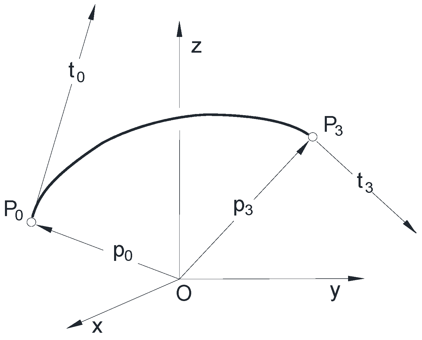
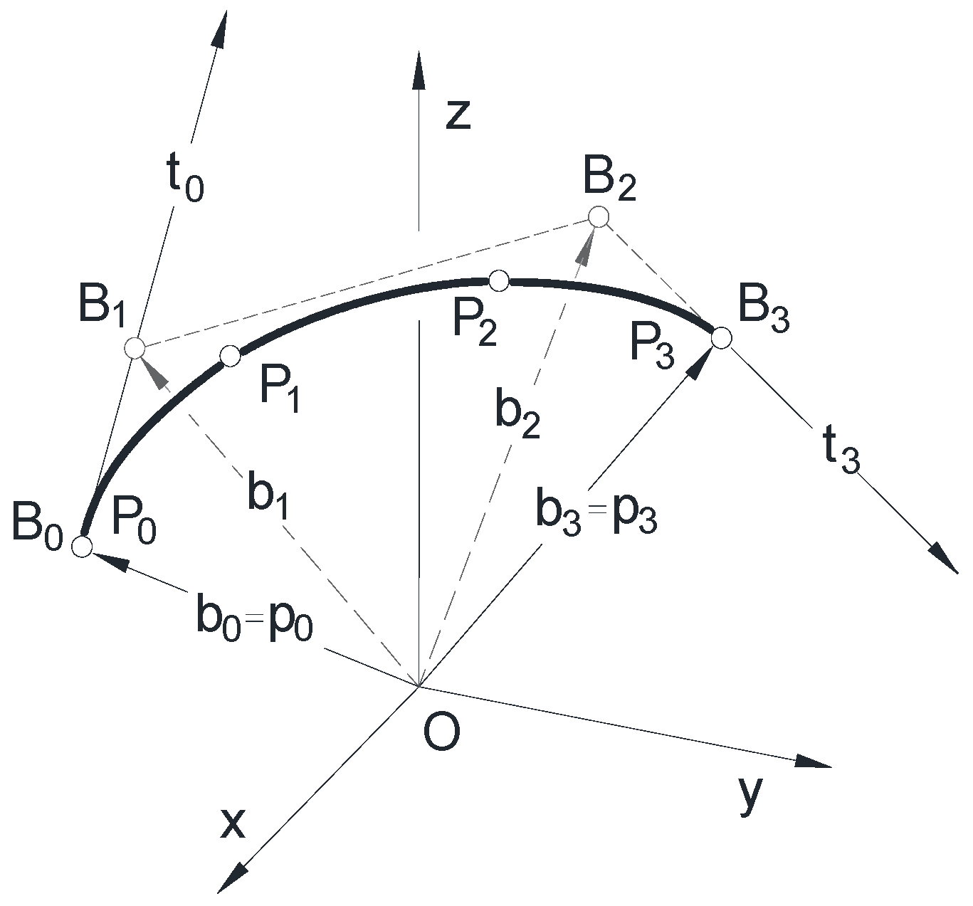
It also applies in this case that if none of the tangents of the curve are in the profile direction, then any part of the curve of the 3D Euclidean space can certainly be clearly reconstructed from only two mutually perpendicular orthogonal projections, namely the representation of any part of the curve is bijective. The examination of the spatial curve was carried out in the case of the third-order curve. Let the position vectors p₀ and p₃ pointing to the starting and ending points of the curve P₀ and P₃ be given, as well as the corresponding starting and ending tangent vectors t₀ and t₁, as shown in Figure 23.

The third-order parametrically determined polynomial form of the spatial curve is suitable for the examination of the reconstructibility from its images. The equation of the third-order curve, characterized by the parameter u can be written into the following form

$$r\left(u\right)=a_3·u^3+a_2·u^2+a_1·u+a_0$$

(51)

where practically u ∈ [0,1], and the derived tangent vectors are given in the form

$$r_{\mathrm{e}}\left(u\right)=e_1·u^2+e_2·u+e_3$$

(52)

Because of the condition u ∈ [0,1], the identities are obtained

$$\left.\begin{array}{l}{a}_0=p_0\\ a_1=p_3\\ a_2=-3\cdot p_0+3\cdot p_3-2\cdot t_0-t_3\\ a_3=2\cdot p_0-2\cdot p_3+t_0+t_3\end{array}\right\}$$

(53)

Accordingly, the tangent vectors will be

$$\left.\begin{array}{l}{e}_1=6\cdot p_0-6\cdot p_3+3\cdot t_0+3t_3\\ e_2=-6\cdot p_0+6\cdot p_3-4\cdot t_0-2\cdot t_3\\ e_3=t_0\end{array}\right\}$$

(54)

Tangent vectors pass through the origin point O. Any profile plane on which none of the tangent vectors lie determines a Monge projection, which always results in a bijective representation of the given curve. The normal vectors n(n_x, n_y, n_z) of the planes containing any of the tangent vectors are perpendicular to the tangent vectors lying in it; therefore, the following equation is fulfilled, namely

$$n·r_{\mathrm{e}}\left(u\right)=0$$

(55)

that can be formed in the following form

$${\mathrm{n}}_{\mathrm{x}}{·\mathrm{r}}_{\mathrm{ex}}\left(u\right){ + \mathrm{n}}_{\mathrm{y}}{·\mathrm{r}}_{\mathrm{ey}}\left(u\right){ + \mathrm{n}}_{\mathrm{z}}{·\mathrm{r}}_{\mathrm{ez}}\left(u\right) = 0$$

(56)

as well as

$$\left({\mathrm{n}}_{\mathrm{x}}{·\mathrm{e}}_{1\mathrm{x}}{ + \mathrm{n}}_{\mathrm{y}}{·\mathrm{e}}_{1\mathrm{y}}{ + \mathrm{n}}_{\mathrm{z}}{·\mathrm{e}}_{1\mathrm{z}}\right) · u^2 + \left({\mathrm{n}}_{\mathrm{x}}{·\mathrm{e}}_{2\mathrm{x}}{ + \mathrm{n}}_{\mathrm{y}}{·\mathrm{e}}_{2\mathrm{y}}{ + \mathrm{n}}_{\mathrm{z}}{·\mathrm{e}}_{2\mathrm{z}}\right) · u + \left({\mathrm{n}}_{\mathrm{x}}{·\mathrm{e}}_{3\mathrm{x}}{ + \mathrm{n}}_{\mathrm{y}}{·\mathrm{e}}_{3\mathrm{y}}{ + \mathrm{n}}_{\mathrm{z}}{·\mathrm{e}}_{3\mathrm{z}}\right)=0$$

(57)

To specify the conditions of bijective Monge projections, it is necessary to determine the vectors n(n_x, n_y, n_z), for which the quadratic equation for the parameter u has no solution.

In the following, the vectors n(n_x, n_y, n_z) in Equation (57) must be determined, for which the quadratic equation with respect to the u parameter has no solution in the case of the specified e_ij (i = 1,2,3 and j = x,y,z) values. The profile planes determined by such normal vectors do not have a tangent to the examined curve, therefore in the Monge projections related to these profile planes the curve representation is bijective. For the normal vector of the profile plane of all bijective Monge projections, the value of the discriminant of equality (57) is negative, that is

$${\left({\mathrm{n}}_{\mathrm{x}}{·\mathrm{e}}_{2\mathrm{x}}{ + \mathrm{n}}_{\mathrm{y}}{·\mathrm{e}}_{2\mathrm{y} }{ + \mathrm{n}}_{\mathrm{z}}{·\mathrm{e}}_{2\mathrm{z}}\right)}^2-4·\left({\mathrm{n}}_{\mathrm{x}}{·\mathrm{e}}_{1\mathrm{x}}{ + \mathrm{n}}_{\mathrm{y}}{·\mathrm{e}}_{1\mathrm{y}}{ + \mathrm{n}}_{\mathrm{z}}{·\mathrm{e}}_{1\mathrm{z}}\right)·\left({\mathrm{n}}_{\mathrm{x}}{·\mathrm{e}}_{3\mathrm{x}}{ + \mathrm{n}}_{\mathrm{y}}{·\mathrm{e}}_{3\mathrm{y}}{ + \mathrm{n}}_{\mathrm{z}}{·\mathrm{e}}_{3\mathrm{z}}\right)<0$$

(58)

For the sake of clarity, a reference [50], proposes writing the constant values of the condition of the negative discriminant in the forms c_i and c_ij (i,j = 1,2,3) giving a new form of the inequality:

$${\mathrm{c}}_1·{\mathrm{n}}_{\mathrm{x}}^2+{\mathrm{c}}_2·{\mathrm{n}}_{\mathrm{y}}^2+{\mathrm{c}}_3·{\mathrm{n}}_{\mathrm{z}}^2+{\mathrm{c}}_{12}·{\mathrm{n}}_{\mathrm{x}}·{\mathrm{n}}_{\mathrm{y}}+{\mathrm{c}}_{13}·{\mathrm{n}}_{\mathrm{x}}·{\mathrm{n}}_{\mathrm{z}}+{\mathrm{c}}_{23}·{\mathrm{n}}_{\mathrm{y}}·{\mathrm{n}}_{\mathrm{z}}<0$$

(59)

Monge cuboid points satisfying the equation formed from the inequality in the following way

$${\mathrm{c}}_1{·\mathrm{n}}_{\mathrm{x}}^2{ + \mathrm{c}}_2{·\mathrm{n}}_{\mathrm{x}}^2{ + \mathrm{c}}_1{·\mathrm{n}}_{\mathrm{y}}^2{ + \mathrm{c}}_3{·\mathrm{n}}_{\mathrm{z}}^2{ + \mathrm{c}}_{12}{·\mathrm{n}}_{\mathrm{x}}{·\mathrm{n}}_{\mathrm{y}}{ + \mathrm{c}}_{13}{·\mathrm{n}}_{\mathrm{x}}{·\mathrm{n}}_{\mathrm{z}}{ + \mathrm{c}}_{23}{·\mathrm{n}}_{\mathrm{y}}{·\mathrm{n}}_{\mathrm{z}}=0$$

(60)

separate the points resulting in bijective and nonbijective representations.

According to another reference [49], when α, β, γ ≠ 0, π, π/2, the reconstruction is ensured with the directions of the projector lines determined by the directed angles corresponding to the following condition

$$\left.\begin{array}{l}{c}_1· {\left(\mathrm{tg}\alpha ·\mathrm{ctg}\gamma + \mathrm{tg}\beta +{\mathrm{tg}\alpha ·\mathrm{tg}}^2\beta \cdot \mathrm{ctg}\gamma \right)}^2/{\left(-\mathrm{ctg}\alpha -\mathrm{tg}\beta \cdot \mathrm{ctg}\gamma -\mathrm{tg}\alpha \right)}^2+\\ c_2·{\left(\mathrm{tg}\alpha ·\mathrm{tg}\beta -\mathrm{ctg}\gamma \right)}^2/{\left(-\mathrm{ctg}\alpha -\mathrm{tg}\beta \cdot \mathrm{ctg}\gamma -\mathrm{tg}\alpha \right)}^2+{\mathrm{c}}_3+\\ {\mathrm{c}}_{12}·\left(\mathrm{tg}\alpha ·\mathrm{ctg}\gamma +\mathrm{tg}\beta +{\mathrm{tg}\alpha ·\mathrm{tg}}^2\beta \cdot \mathrm{ctg}\gamma \right)\cdot \left(\mathrm{tg}\alpha ·\mathrm{tg}\beta -\mathrm{ctg}\gamma \right)/\\ {\left(-\mathrm{ctg}\alpha -\mathrm{tg}\beta \cdot \mathrm{ctg}\gamma -\mathrm{tg}\alpha \right)}^2+\\ {\mathrm{c}}_{13}·\left(\mathrm{tg}\alpha · \mathrm{ctg}\gamma + \mathrm{tg}\beta +{\mathrm{tg}\alpha · \mathrm{tg}}^2\beta \cdot \mathrm{ctg}\gamma \right)/\left(-\mathrm{ctg}\alpha -\mathrm{tg}\beta \cdot \mathrm{ctg}\gamma -\mathrm{tg}\alpha \right)+\\ {\mathrm{c}}_{23}·\left(\mathrm{tg}\alpha · \mathrm{tg}\beta -\mathrm{ctg}\gamma \right)/\left(-\mathrm{ctg}\alpha -\mathrm{tg}\beta \cdot \mathrm{ctg}\gamma -\mathrm{tg}\alpha \right)<0\end{array}\right\}$$

(61)

3. Result and Application in Mechanical Engineering Practice

One of the special scientific research areas of our Worm School of Science, which deals with the geometry of the tooth surfaces of helicoid surfaces and connected gears [51,52,53,54,55,56], as well as the machining geometry approach to the mathematical determination in their production, is the analysis of the production geometry development in the case of the cylindrical worm with a circular profile in axial section as shown in Figure 24, and the gear connected to it.

The very complicated machining process of the gear tooth surface can be facilitated by enveloping the surface of the worm connected to the gear. This may be done by means of direct motion mapping (Figure 25), which can be performed with the worm cutter formed from the worm.

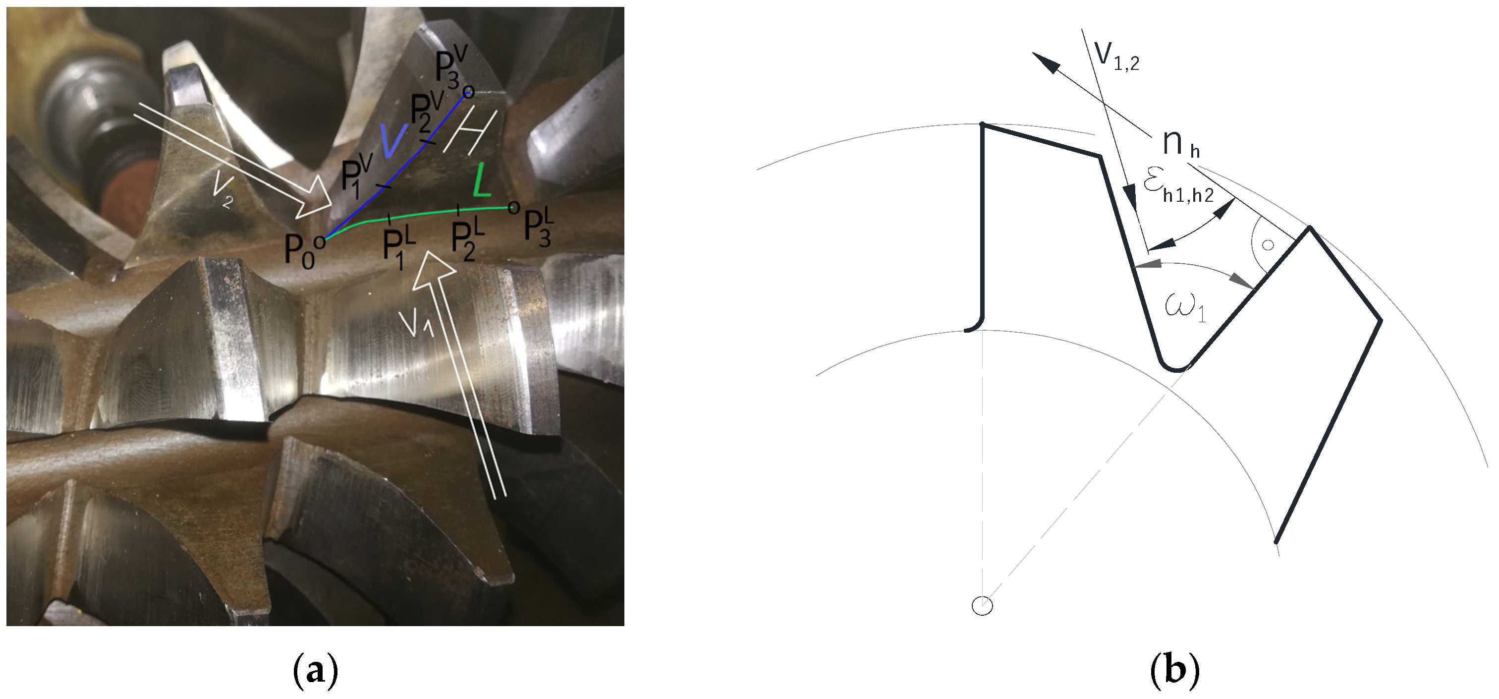
In order to increase the precision of the production, the wear of the hob can be monitored with CCD cameras during production. The use of two CCD cameras perpendicular to each other to facilitate precise monitoring utilizes the theoretical base provided by Monge mapping. In addition to the ratios of the tool edge size and the distance from the cameras, the geometric corrections to eliminate distortion were performed using the “Contour2” program on the digitized images, which can be considered as the two projection images [52]. The cutting edge may be considered as a cubic curve with its digitized images taken with the two CCD cameras serving as images projected onto the first and second image planes in Monge mapping. During the reconstruction from the images of the Monge mapping, it is indifferent which image is the first and which is the second, i.e., the images are interchangeable, i.e., they have symmetry properties, which also applies to the numbering of the CCD cameras. The wear test of the cutting-edge curve with CCD cameras can only be performed if any part of the curve can be clearly reconstructed from its two images.

As shown in Figure 26a, reconstructibility must be ensured not only for the cutting edge, but also for the intersected arc between the foot cylinder and the tooth face surface to set the tool into the same position for the testing.

The appropriate form of examination of the cutting-edge curve, which has changed as a result of the operation, is the interpolating third-order Bezier curve, whose connection with the Hermite arc is shown in Figure 27.

It is advisable to select the cutting-edge points P₃ and P₀ on the addendum and root cylinder, so that the points P₂ and P₁ between them could be defined proportionally to their distance from the axis. The interpolating Bezier curve has four selected points with their position vectors p₀, p_1, p₂, p₃ on the cutting edge of the hob, and its parameters u₀, u₁, u₂, u₃ satisfy the condition u_i ≠ u_j, if i ≠ j, as well as u₀ = 0 and u₃ = 1. The coordinates of the position vectors b₀, b_1, b₂, b₃ of the control points B₀, B_1, B₂, B₃ have to be calculated, which will determine the interpolation Bezier curve passing through the selected points so that the following equation is fulfilled

$$\begin{array}{cc}b\left(u_{\mathrm{i}}\right)=p_{\mathrm{i}}& \left(\mathrm{i}=0,\dots ,3\right)\end{array}$$

(62)

Bezier curve using the Bernstein polynomials is

$$\begin{array}{ccc}b\left(u\right)={\displaystyle {\displaystyle \sum }_{\mathrm{j}=0}^{\mathrm{n}}}{\mathrm{B}}_{\mathrm{j}}^{\mathrm{n}}\left(u\right) b_{\mathrm{j}}& {\mathrm{B}}_{\mathrm{j}}^{\mathrm{n}}\left(u\right)=\left(\begin{array}{c}\mathrm{n}\\ \mathrm{j}\end{array}\right)u^{\mathrm{j}}{\left(1-u\right)}^{\mathrm{n}-\mathrm{j}}& \left(\mathrm{i}=0,\dots ,3\right)\end{array}$$

(63)

Because of the Bezier curve passes through the selected points P₀, P₁, P₂ and P₃, it can be defined by the following equation

$$b\left(u\right)={\displaystyle {\displaystyle \sum }_{\mathrm{j}=0}^{\mathrm{n}}}{\mathrm{B}}_{\mathrm{j}}^{\mathrm{n}}\left(u\right) b_{\mathrm{j}} \left(\mathrm{j}=0,\dots ,3\right)$$

(64)

Using Equation (62) the following linear inhomogeneous equation system can be created

$$\left[\begin{array}{c}{p}_0\\ p_1\\ p_2\\ p_3\end{array}\right]=\left[\begin{array}{cccc}{B}_0^3\left(u_0\right)& B_1^3\left(u_0\right)& B_2^3\left(u_0\right)& B_3^3\left(u_0\right)\\ B_0^3\left(u_1\right)& B_1^3\left(u_1\right)& B_2^3\left(u_1\right)& B_3^3\left(u_1\right)\\ B_0^3\left(u_2\right)& B_1^3\left(u_2\right)& B_2^3\left(u_2\right)& B_3^3\left(u_2\right)\\ B_0^3\left(u_3\right)& B_1^3\left(u_3\right)& B_2^3\left(u_3\right)& B_3^3\left(u_3\right)\end{array}\right]·\left[\begin{array}{c}{b}_0\\ b_1\\ b_2\\ b_3\end{array}\right]$$

(65)

Calculation had to be performed separately for each coordinate, and its clear solution was the result of the condition specified by us. Thus, the b_i vectors (i = 0,…,3) pointing to control points B₀, B_1, B₂, B₃ of the Bezier curve passing through the selected points P₀, P_1, P₂, P₃ can be calculated based on Equation (65). The relationship between the p₀, p_1, p₂, p₃ position vectors of the control points of the Bezier curve and the position vectors of the start and end points p₀ and p₃, as well as the start and end tangents t₀ and t₃ of the Hermite arc can be characterized by the following relations based on the literature [49] and according to the guidance of Figure 27.

$$\left.\begin{array}{l}{p}_0=b_0\\ p_3=b_3\\ t_0=3\cdot b_1-3\cdot b_0\\ t_3=3\cdot b_3-3\cdot b_2\end{array}\right\}$$

(66)

According to our previous analyses [42], the third-degree Bezier curve approaches the cutting edge within the permitted tolerance zone, if the four points of the cutting edge are selected proportionally between the addendum and dedendum cylinder to specified the interpolating Bezier curve, and these were parameterized in proportional length of chord. The inequality (61) varies according to the coordinates of the points of the cutting edge. The CCD cameras positioned using these coordinates with defined directed angles can make in principle produce reconstructable images of the cutting edge.

In the field of view of the CCD cameras positioned according to inequality (61), additional conditions should be formulated for the nearby hob tooth surfaces also require the formulation of.

In addition, a third condition is discussed in this article, which eliminates the projector lines that do not reach in the axis direction the examined cutting edge due to the next hob tooth. If the normal vector n_h of the face surface is determined from the coordinates of the points P₃ and P₀ measured on the cutting edge, as well as the coordinates of the points L₃ and L₀ measured on the root cylinder curve by the cross product of the difference vectors of the position vectors pointing to the points according to the following relation

$$n_{\mathrm{h}}=\left(p_3-p_0\right)\times \left(l_3-l_0\right)$$

(67)

then a strong condition has been established. The angles between the n_h normal vector and the v₁ and v₂ direction vectors of the projector lines can be determined as follows

$$\arccos \left(n_{\mathrm{h}}\cdot v_1/\left|n_{\mathrm{h}}\right|\cdot \left|v_1\right|\right)={\mathsf{\epsilon }}_{\mathrm{h}1}$$

(68)

and

$$\arccos \left(n_{\mathrm{h}}\cdot v_2/\left|n_{\mathrm{h}}\right|\cdot \left|v_2\right|\right)={\mathsf{\epsilon }}_{\mathrm{h}2}$$

(69)

Furthermore, the angles between the face surface H of the hob tooth and the projector lines v₁ and v₂ projecting into the direction of the axis, can have a maximum value ω₁ as shown in Figure 26b). This means that the minimum value of the angles ε_h1 and ε_h2 between the direction vectors of the projector lines and the normal vector n_h must be ${90}^{\mathrm{o}}-{\mathsf{\omega }}_1$ for the chip groove angle of size ω₁, as it can be written as

$${\mathsf{\epsilon }}_{\mathrm{h}1},{\mathsf{\epsilon }}_{\mathrm{h}2}\le {90}^{\circ }-{\mathsf{\omega }}_1$$

(70)

With the visualized procedure, a solution can be selected simultaneously from the subset of solutions in the case of three unknown inequalities, as shown in Figure 28.

During the machining of parts, this procedure will facilitate the continuous monitoring of changes in the size and shape of the cutting edge of the tool, which affects the quality of the machined surface.

4. Discussion

The computer technology evolution greatly reduced the cost of designing and prototyping mechanisms. Software packages available on the market and the exponential development of computers offer a huge number of possibilities while results can be achieved in a much shorter time. The primary task of those engineers who undertake the whole process from design to implementation is to select compatible software packages that meets industrial requirements. During the design process of the drives, by examining the effect of several possible modifications of the geometric parameters of its elements (production accuracy, quality, standard profile angle and gear width), the optimal solution can be selected using a computer program based on the Taguchi method, which is an optimization procedure based a numerous steps of planning, transacting and interpreting results of matrix tests to determine the most suitable value of the control parameters [57].

A wide selection of tools is available for surface measurement, such as mechanical stylus profilometers, noncontact optical ones, and scanning probe microscopes to take a cross-sectional contour of the air topography data of the investigated surfaces [58]. Several recent reports deal with examinations on optical measurements [59], mainly with diffractive relief structures [60] as well as with interference microscopy [61] and confocal and spiral scanning [62], factoring in the comparative papers on various technologies [63]. Some researchers have also discussed the comparability of the surface parameters resulting from the profile and the areal measurements [64,65].

Each of these software’s means of communication between designers and constructors rely on Monge’s two-view representations of the 3D [66]. The importance of the production geometry is also demonstrated, for example, by the fact that in order to improve the operating characteristics of hypoid gears, which can be achieved by optimally changing the related tooth surfaces, that can be realized by modifying the settings of the machine tool. The purposes of the multi-objective optimization procedure created with numerical methods were to minimize the maximum contact pressure of the teeth, the transmission error, and the average temperature of the gears in their contact zone, and to maximize the mechanical efficiency in the case of hypoid gear drives [67]. The wear resistance and service life of cutting tools are also affected by the tribological behavior of the different coatings produced with different production parameters [68]. The design and construction of most mechanisms require a unique approach due to various considerations, which represents a constant challenge for today’s engineers. A lot of procedures have been prepared to generate the production geometry of machining tools for helicoidal surfaces with constant thread pitch based on the principle of mutual envelopment of surfaces according to the theorems of Olivier and Gohman. A numerical solution suitable for profiling the grinding wheels to generate the helicoidal surface of the threaded ball-nut motion conversion mechanism is based on the theory of derivation and intersection of surfaces. The points of the approximation tool profile accepted as the final result are the intersection curve points of the derivative surface and the workpiece surface, determined by an initial value problem of an ordinary differential equation system. The smallness of the deviation of the resulted approximation tool profile from the geometrically defined surface, namely its accuracy according to engineering terminology, also depends on the density of the calculated points [69].

The determination of the points of theoretical tooth surfaces for various drives components must be produced according to the machining process with a mathematical toolbox aimed at the format suitable for the purpose [70]. The theoretical tooth surface can be meshed by any number of its discrete points in the mathematical model made for checking the accuracy. Manufacturing accuracy, referring to the quality of the machined surface, is usually measured with a coordinate measuring machine, establishing the difference between the coordinates of the theoretical tooth surface points treated as a reference and the coordinates of the manufactured tooth surface points measured with the coordinate measuring machine. All this can be reviewed in the case of the creation of a mathematical model describing the machining of the tooth surfaces of bevel gears with curved teeth, where the coordinates of the known points of the theoretical tooth surface in the grid points are the reference values on the coordinate measuring machine, which can be compared with the coordinates of the points measured on the manufactured surface [71].

Using exact geometric construction, an interesting motion geometrical result has been published at the operating of the roller freewheel fulfilling the base requirement, that the housing profile, and the hub should create a taper gap, so the roller center has to be functional along a logarithmic spiral [72].

The geometrical design of the drive pair components has a significant effect on achieving the desired efficiency, since the correct formation of the lubricating wedge is essential in terms of reducing friction and wear during operation [73]. Many forward-looking developments have been also made using graphical systems for the further development of technical tools [74]. The simulation and movement study of the Mechanical Integrator 3D Model can also help to understand the processes [75].

When studying the production geometry of the drive pairs, tests can also be carried out regarding the profile error-free production [76] in order to avoid undercutting. Several geometry-based methods can be used to increase efficiency, such as the coordinate geometry toolbox supplemented with numerical methods [77] and simulation and analytical tools [78] for different type of drives.

By modeling the targeted theoretical tooth sides of the complicated worm gear that fits the cylindrical worm in the three-dimensional CAD software, and by manufacturing the worm gear using a CAM process, and then comparing the contact patterns of the experimental and analytical teeth, it can be concluded that they can be considered to be of the same approximation as required in the industry, and as a result, the manufacturing method has been already validated [79]. The selection of projections is decisive for examining changes in shape and kinematic geometry during machining with high-feed face milling, since at low feed, the effect of the material forming of the side edge has been the most critical, the chip becomes deformed perpendicular to it, while the primary part of chip removal gradually moves to an edge perpendicular to the tool axis as the feed increases. For effective chip removal, the two edges can be tested separately and together, for which a mathematical model was carried out to create the basis of the (Finite Element Method) FEM examinations [80]. The reliability of finite element simulations and other methods strongly depends on the applied constitutive models [81]. When forming materials with higher strength in the automotive industry, by increasing fuel efficiency, vehicles also achieve the necessary safety standards, taking into account that during production, the geometry also varies depending on the properties of the material [82].

An important part of our research work was also the examination of the profile distortions of the grinding wheel during worm surface machining with a CCD camera [83], which was able to recognize the contour of the working surface of the grinding wheel, from which it was possible to make decisions about the need for re-sharpening.

5. Conclusions

In the course of our research, during the machining of the worm gear with a hob, a new mathematical procedure has been developed for positioning the CCD cameras with mathematical precision to ensure that the cutting-edge curve can be reconstructed from digitized images for wear measurement. The cutting-edge wear tester must be in the same position for each measurement. To set the hob into one position, a surface element had to be selected that does not take part in the machining; therefore, its shape does not change. The cutting curve of the root cylinder and the face surface of the hob tooth are suitable for this purpose.

At the same time, by positioning CCD cameras, it is also necessary to ensure the reconstruction of the intersection curve between the face surface of the hob tooth and the bottom cylinder. In order to simultaneously correctly adjust the CCD cameras to the intersected curve between the tooth surface and the root cylinder and to the curve of the cutting edge, so that they only have to be reconstructed from two images taken as perpendicular projections, the data can be derived from the points of the bijective subset of the Monge cuboid with respect to both curves. The directed angles belonging to the point chosen from the bijective subsets of the Monge cuboid determine the directions, in which the CCD cameras should be positioned. This procedure has been developed to measure the wear of the cutting edge of the hob during processing, with which the spatial deformation of the cutting-edge curve can be reconstructed only from digitalized images taken with two CCD cameras using the methods of constructive descriptive geometry. A new third condition has been formulated mathematically, according to which the next tooth of the hob should not be an obstruction to record the images taken of the cutting edge, that is, the cameras facing to the direction of the axis could reach the cutting edge. To determine the condition to solve this problem, the relationship between the normal of the face surface of the hob tooth and the projector lines has been determined.

The aim of this endeavor was to make abstract mathematical ideas useful for practical implementations. The theoretical limitation of this study is that it only deals with edge curves, and the mechanical limitation is the dependence on the quality of the tools.

An open question in my future geometrically oriented research is how the parameters defining Monge mappings should be defined in the projective model instead of the Euclidean spatial model, so that their set shows additional advantages.

References

- Stachel, H. The status of today’s Descriptive Geometry related education (CAD/CG/DG) in Europe. J. Graph. Sci. Jpn. 2007, 41 (Suppl. S1), 15–20. [Google Scholar] [CrossRef]
- Forgó, Z.; Tolvaly-Roșca, F.; Pásztor, J.; Kővári, A. Energy Consumption Evaluation of Active Tillage Machines Using Dynamic Modelling. Appl. Sci. 2021, 11, 6240. [Google Scholar] [CrossRef]
- Suzuki, K. Traditional Descriptive Geometry Education in the 3D-CAD/CG Era. J. Geom. Graph. 2014, 18, 249–258. Available online: https://www.heldermann-verlag.de/jgg/jgg18/j18h2suzu.pdf (accessed on 16 November 2014).
- Tozzi, A.; Mariniello, L. Unusual Mathematical Approaches Untangle Nervous Dynamics. Biomedicines 2022, 10, 2581. [Google Scholar] [CrossRef]
- Guth, P.L.; van Niekerk, A.; Grohmann, C.H.; Muller, J.P.; Hawker, L.; Florinsky, I.V.; Gesch, D.; Reuter, H.I.; Herrera-Cruz, V.; Riazanoff, S.; et al. Digital Elevation Models: Terminology and Definitions. Remote Sens. 2021, 13, 3581. [Google Scholar] [CrossRef]
- Szarvas, B.; Virág, Z. Seismic effects of rock blasting in the Erdőbénye andesite quarry. Multidiscip. Sci. 2021, 11, 159–169. [Google Scholar] [CrossRef]
- Miklós, R.; Lénárt, L.; Darabos, E.; Kovács, A.; Pelczéder, Á.; Szabó, N.P.; Szűcs, P. Karst water resources and their complex utilization in the Bükk Mountains, northeast Hungary: An assessment from a regional hydrogeological perspective. Hydrogeol. J. 2020, 28, 2159–2172. [Google Scholar] [CrossRef]
- Yin, Q.; Chen, Z.; Zheng, X.; Xu, Y.; Liu, T. Sliding Windows Method Based on Terrain Self-Similarity for Higher DEM Resolution in Flood Simulating Modeling. Remote Sens. 2021, 13, 3604. [Google Scholar] [CrossRef]
- Kundrák, J.; Nagy, A.; Markopoulos, A.P.; Karkalos, N.E. Investigation of surface roughness on face milled parts with round insert in planes parallel to the feed at various cutting speeds. Cut. Tools Technol. Syst. 2019, 91, 87–96. [Google Scholar] [CrossRef]
- Cepova, L.; Cep, R.; Chalko, L.; Dvorackova, S.; Trochta, M.; Rucki, M.; Beranek, L.; Mizera, O.; Chyshkala, V. The Effect of Cutting Tool Geometry on Surface Integrity: A Case Study of CBN Tools and the Inner Surface of Bearing Rings. Appl. Sci. 2023, 13, 3543. [Google Scholar] [CrossRef]
- Cabezas, S.; Hegedűs, G.; Bencs, P. Transient heat convection analysis of a single rod in air cross-flow. Pollack Period. 2023, 18, 23–28. [Google Scholar] [CrossRef]
- Cvetković, I.D.; Stojićević, M.D.; Stachel, H.; Milićević, R.G.; Popkonstantinović, B.D. The Man who Invented Descriptive Geometry. FME Transactions 2019, 47, 331–336. [Google Scholar] [CrossRef]
- Bucur, C.; Máté, M. Theoretical Peculiarities Regarding the Definition and Representation of the Rolling Surfaces for Chain Transmission. Procedia Eng. 2017, 181, 206–213. [Google Scholar] [CrossRef]
- Hervé, J.M. Théodore Olivier (1793–1853). Disting. Fig. Mech. Mach. Sci. Hist. Mech. Mach. Sci. 2007, 1, 295–318. [Google Scholar] [CrossRef]
- Glaeser, G.; Stachel, H. Kinematics—Geometry of Motion. In Open Geometry: OpenGL® + Advanced Geometry; Springer: Berlin/Heidelberg, Germany, 1999; Volume 451, pp. 229–267. [Google Scholar] [CrossRef]
- Körei, A.; Szilágyi, S. Displaying Parametric Curves with Virtual and Physical Tools. Teach. Math. 2022, 25, 61–73. [Google Scholar] [CrossRef]
- Maláková, S.; Urbanský, M.; Fedorko, G.; Molnár, V.; Sivak, S. Design of Geometrical Parameters and Kinematical Characteristics of a Non-circular Gear Transmission for Given Parameters. Appl. Sci. 2021, 11, 1000. [Google Scholar] [CrossRef]
- Bendefy, A.; Horák, P. Gear pair generation with the method of transposed lines of action. In Proceedings of the 14th International Design Conference, DESIGN 2016, Zagreb, Croatia, 16–19 May 2016; pp. 129–136. Available online: https://www.designsociety.org/publication/38822/GEAR+PAIR+GENERATION+WITH+THE+METHOD+OF+TRANSPOSED+LINES+OF+ACTION (accessed on 31 October 2023).
- Bendefy, A.; Horák, P. Cylindrical Gears with Changing Ratio. Period. Polytech. Mech. Eng. 2017, 61, 130–134. [Google Scholar] [CrossRef]
- Benotsmane, R.; Dudás, L.; Kovács, G. Newly Elaborated Hybrid Algorithm for Optimization of Robot Arm’s Trajectory in Order to Increase Efficiency and Provide Sustainability in Production. Sustainability 2021, 13, 8193. [Google Scholar] [CrossRef]
- Balajti, Z. Development of the Manufacturing Geometry of Conical and Cylindrical Worms by Analyzing of Their Axoids. Manuf. Technol. 2020, 20, 3–10. [Google Scholar] [CrossRef]
- Güler, E. Generalized Helical Hypersurfaces Having Time-like Axis in Minkowski Spacetime. Universe 2022, 8, 469. [Google Scholar] [CrossRef]
- Balajti, Z.; Mándy, Z. Proposed solution to eliminate pitch fluctuation in case of conical screw surface machining by apex adjustment. Procedia Manuf. 2021, 55, 266–273. [Google Scholar] [CrossRef]
- Bonata, C.I.; Bolos, V. The mathematical model of generating kinematic for the worm face gear with modified geometry. Procedia Technol. 2014, 12, 442–447. [Google Scholar] [CrossRef]
- Hogyai, N.; Máté, M.; Tolvaly-Roșca, F.; Drăgoi, M.V. Peculiarities of the Grinding Process of a Gear Hob Helical Rake Face. Acta Univ. Sapientiae Electr. Mech. Eng. 2021, 13, 39–51. [Google Scholar] [CrossRef]
- Tolvaly-Roșca, F.; Forgó, Z.; Máté, M. Evaluation of a Mixed CAD Gear Modeling from Time and Precision Point of View. Procedia Technol. 2015, 19, 28–33. [Google Scholar] [CrossRef]
- Ábrahám, G.; Wenzelné Gerőfy, K.; Antal, Á.; Kovács, G. Technical Optics, 1st ed.; Institute of Mechatronics, Optics, and Mechanical Engineering Informatics, Budapest University of Technology and Economics: Budapest, Hungary, 2015; p. 308. ISBN 978-963-313-202-9. Available online: https://mogi.bme.hu/TAMOP/muszaki_optika/index.html (accessed on 31 October 2023).
- Csoba, I.; Kunkli, R. Rendering algorithms for aberrated human vision simulation. Vis. Comput. Ind. Biomed. Art 2023, 6, 5. [Google Scholar] [CrossRef] [PubMed]
- Prado-Velasco, M.; García-Ruesgas, L. Intersection and Flattening of Surfaces in 3D Models through Computer-Extended Descriptive Geometry (CeDG). Symmetry 2023, 15, 984. [Google Scholar] [CrossRef]
- Papp, G.; Papp, I.; Kunkli, R. Three-dimensional connection visualization based on tabular data. In Proceedings of the 8th IEEE International Conference on Cognitive Infocommunications (CogInfoCom), Debrecen, Hungary, 11–14 September 2017; pp. 289–290. [Google Scholar] [CrossRef]
- Ding, Z.; Liu, S.; Liao, L.; Zhang, L. A digital construction framework integrating building information modeling and reverse engineering technologies for renovation projects. Autom. Constr. 2019, 102, 45–58. [Google Scholar] [CrossRef]
- Papp, I.; Zichar, M. 3D Modelling and Printing Interpreted in Terms of Cognitive Infocommunication. In Cognitive Infocommunications, Theory and Applications Topics in Intelligent Engineering and Informatics; Springer: Berlin/Heidelberg, Germany, 2019; Volume 13. [Google Scholar] [CrossRef]
- Bartonek, D.; Buday, M. Problems of Creation and Usage of 3D Model of Structures and Theirs Possible Solution. Symmetry 2020, 12, 181. [Google Scholar] [CrossRef]
- Benardos, P.; Vosniakos, G.C. Removed material volume calculations in CNC milling by exploiting CAD functionality. Int. J. Comput. Aided Eng. Technol. 2018, 10, 495–503. [Google Scholar] [CrossRef]
- Dudás, I.; Balajti, Z. Modelling and development for describing the bearing pattern of spiroid drives. In Proceedings of the Sixth IASTED International Conference on Robotics and Applications, Cambridge, MA, USA, 31 October–2 November 2005; pp. 203–208, ISBN 0-88986-521-3. Available online: https://www.actapress.com/Abstract.aspx?paperId=22994 (accessed on 31 October 2023).
- Bodzás, S.; Békési, Z.; Kertész, J.; Szorcsik, T. The CAD Modelling Possibilities of Gear Pairs by Two Ways in the Mechanical Engineering Practice. Int. J. Eng. Manag. Sci. 2021, 6, 205–219. [Google Scholar]
- Kundrák, J.; Felhő, C.; Nagy, A. Analysis and Prediction of Roughness of Face Milled Surfaces using CAD Model. Manuf. Technol. 2022, 22, 558–572. [Google Scholar] [CrossRef]
- Máté, M.; Tolvaly-Roșca, F.; Hodgyai, N.; Drăgoi, M.V. A new approach of defining the grinding wheel profile of the Gear Hob’s Rake Face. In Proceedings of the IEEE Joint 22nd International Symposium on Computational Intelligence and Informatics and 8th International Conference on Recent Achievements in Mechatronics, Automation, Computer Science and Robotics (CINTI-MACRo 2022), Budapest, Hungary, 21–22 November 2022. [Google Scholar] [CrossRef]
- Hogyai, N.; Drăgoi, M.V.; Tolvaly-Roșca, F.; Máté, M. About the Grinding of Gear Hob’s Rake Face. Pap. Tech. Sci. Int. Sci. Ser. Transylv. Mus. Soc. 2022, 16, 31–35. [Google Scholar] [CrossRef]
- Dudás, I. The Theory and Practice of Worm Gear Drives; Penton Press: London, UK, 2000. [Google Scholar]
- Olivier, T. Theorie Geometrique Engrenager; Maurice Daumas: Paris, France, 1842; Available online: https://archive.org/details/thoriegomtrique01olivgoog/page/n117/mode/2up (accessed on 31 October 2023).
- Balajti, Z. Development of Production Geometry of Kinematical Drive Pairs. Ph.D. Thesis, University of Miskolc, Miskolc, Hungary, 2007; p. 171. Available online: http://midra.uni-miskolc.hu/document/5519 (accessed on 31 October 2023). (In Hungarian).
- Bodzás, S. Manufacturing of spur gears having normal teeth on different pressure angles by module disc milling cutter. Int. Rev. Appl. Sci. Eng. 2022, 13, 321–334. [Google Scholar] [CrossRef]
- Tomori, Z. An Optimal Choice of Profile Shift Coefficients for Spur Gears. Machines 2021, 9, 106. [Google Scholar] [CrossRef]
- Meng, Q.; Zhao, Y.; Yang, Z. Curvature interference characteristic of conical worm gear. Forsch Ingenieurwes 2019, 83, 759–773. [Google Scholar] [CrossRef]
- Pavlenko, S.; Mascenik, J.; Krenicky, T. Mathematical Modeling of Drive and Dynamic Load of Teeth of Cylindrical Worm Gear, 2022. In Sustainable Management of Manufacturing Systems in Industry 4.0, 1st ed.; James, M., Ed.; Springer: Cham, Switzerland, 2007; Volume 3, pp. 61–84. [Google Scholar] [CrossRef]
- Balajti, Z. Examination and adjustment of bearing pattern in case of helicoid drives. Procedia CIRP 2018, 77, 267–270. Available online: https://www.sciencedirect.com/journal/procedia-cirp/vol/77/suppl/C (accessed on 31 October 2023). [CrossRef]
- Dudás, I.; Szentesi, A.; Csapó, B. Measurement of grinding wheel wear with a CCD camera. In Proceedings of the Scientific Session of Young Technicians VI, 167-172, Cluj-Napoca, Romania, 23–24 March 2001; Enikő, B., Ed.; Transilvanian Museum Society: Gundelsheim, Germany, 2001. Available online: https://api.eda.eme.ro/server/api/core/bitstreams/91cc925d-072e-4370-9e76-3af6aaa19e90/content (accessed on 31 October 2023). (In Hungarian).
- Balajti, Z. Theoretical Analysis and Application of the Monge Representation in Engineering Practice; University of Miskolc: Miskolc, Hungary, 2015; 101p, ISBN 978-963-358-097-4. Available online: https://www.researchgate.net/publication/372855431_A_Monge_abrazolas_elmeleti_elemzese_es_alkalmazasa_a_mernoki_gyakorlatban_Miskolc_2015_ISBN_978-963-358-097-4_101_o (accessed on 31 October 2023).
- Balajti, Z.; Dudás, I. The Monge Theorem and Its Application in Engineering Practice. Int. J. Adv. Manufturing Technol. 2017, 91, 739–749. [Google Scholar] [CrossRef]
- Dudás, I.; Bányai, K.; Bodzás, S. Finishing production of spiroid worm shaft by varied center distance and by applying grinding wheel banking angle correction. Int. Rev. Appl. Sci. Eng. 2016, 7, 13–19. [Google Scholar] [CrossRef]
- Dudás, L. Modelling and simulation of a new worm gear drive having point-like contact. Eng. Comput. 2013, 29, 251–272. [Google Scholar] [CrossRef]
- Bodzás, S. Connection analysis of surfaces of conical worm, face gear and tool. Ph.D. Thesis, University of Miskolc, Miskolc, Hungary, 2016; p. 120. Available online: http://midra.uni-miskolc.hu/document/18016/11619.pdf (accessed on 31 October 2023). (In Hungarian).
- Mándy, Z. Intelligent Manufacturing System and Geometrically Exact Manufacture of the Helicoid Surfaces. Ph.D. Thesis, University of Miskolc, Miskolc, Hungary, 2022; p. 105. Balajti, Z., Ed. (In Hungarian). Available online: http://193.6.1.94:9080/JaDoX_Portlets/documents/document_40897_section_38553.pdf (accessed on 31 October 2023). (In Hungarian).
- Ábel, J. Computer Based Constructive Geometric and Analytical Development of the Manufacturing Geometry of Worm Gear Drive Pairs. Ph.D. Thesis, University of Miskolc, Miskolc, Hungary, 2023; p. 99. Balajti, Z., Ed. (In Hungarian). Available online: http://midra.uni-miskolc.hu/document/43049/41118.pdf (accessed on 31 October 2023). (In Hungarian).
- Balajti, Z. Determination of Undercutting Avoidance for Designing the Production Technology of Worm Gear Drives with a Curved Profile. Machines 2023, 11, 56. [Google Scholar] [CrossRef]
- Stanojevic, M.; Stojanovic, B.; Bankovic, N. Analysis of Influential Geometric Parameters on the Safety Factor on the Sides of Gear Pairs in the Gearbox Using Taguchi Method. In Proceedings of the 11th international conference on Quality System Condition for Successful Business and Competitiveness, Kopaonik, Serbia, 17–19 May 2023; Available online: https://www.researchgate.net/publication/373160923_ANALYSIS_OF_INFLUENTIAL_GEOMETRIC_PARAMETERS_ON_THE_SAFETY_FATOR_ON_THE_SIDES_OF_GEAR_PAIRS_IN_THE_GEARBOX_USING_TAGUCHI_METHOD (accessed on 31 October 2023).
- Gao, W.; Haitjema, H.; Fang, F.Z.; Leach, R.K.; Cheung, C.F.; Savio, E.; Linares, J.M. On-machine and in-process surface metrology for precision manufacturing. CIRP Ann. 2019, 68, 843–866. [Google Scholar] [CrossRef]
- Jiao, F.; Liu, L.; Cheng, W.; Li, C.; Zhang, X. Review of optical measurement techniques for measuring three-dimensional topography of inner-wall-shaped parts. Measurement 2022, 202, 111794. [Google Scholar] [CrossRef]
- Lu, W.; Chen, S.; Zhang, K.; Zhai, D. Characterization of diffractive relief structures over large areas by stitching interference microscopic topography. Measurement 2022, 202, 111850. [Google Scholar] [CrossRef]
- Guo, J.; Zhai, D.; Lu, W.; Chen, S. Topography measurement of helical grooves on a hemisphere based on stitching interference microscopy. Opt. Laser Technol. 2022, 152, 108133. [Google Scholar] [CrossRef]
- Ying, R.; Cui, Y.; Huang, J.; Liang, D.; Wang, Y. Precise measurement of surface topography with microstructures based on differential confocal and spiral scanning. Measurement 2021, 184, 110004. [Google Scholar] [CrossRef]
- Leksycki, K.; Królczyk, J.B. Comparative assessment of the surface topography for different optical profilometry techniques after dry turning of Ti6Al4V titanium alloy. Measurement 2021, 169, 108378. [Google Scholar] [CrossRef]
- Schmidt, J.; Thorenz, B.; Schreiner, F.; Döpper, F. Comparison of areal and profile surface measurement methods for evaluating surface properties of machined components. Procedia CIRP 2021, 102, 459–464. [Google Scholar] [CrossRef]
- Svetlik, J.; Baron, P.; Dobransky, J.; Kocisko, M. Implementation of computer system for support of technological preparation of production for technologies of surface processing. In Applied Mechanics and Materials, Proceedings of the ROBTEP 2014: 13th International Conference on Industrial, Service and Humanoid Robotics, High Tatras, Slovakia, 15–17 May 2014; Trans Tech Publications Ltd.: Zurich, Switzerland, 2014; Volume 613, pp. 418–425. ISBN 978-303835202-0. [Google Scholar]
- Stamenović, B.; Stoimenov, M.; Popkonstantinovic, B.; Jeli, Z. Presses for Designing Flexible Pipes Correction, Finite Elements Analysis and Prepearing “G” Code for Construction Elements of Plasma Cutter. In Proceedings of the 4th International Scientific Conference on Geometry and Graphics moNGeometrija, Vlasina, Serbia, 20–22 June 2014; pp. 141–156. Available online: http://mongeometrija.com/konferencije/mongeometrija-2014 (accessed on 31 October 2023).
- Simon, V. Multiobjective optimization of hypoid gears to improve operating characteristics. Mech. Mach. Theory 2019, 146, 905–914. [Google Scholar] [CrossRef]
- Jakab, M.; Ali, O.I.; Gyurika, I.G.; Korim, T.; Telegdi, J. The Tribological Behavior of TiN/TiC CVD Coatings under Dry Sliding Conditions against Zirconia and Steel Counterparts. Coatings 2023, 13, 832. [Google Scholar] [CrossRef]
- Hegedűs, G. Manufacturing Parameters Determination on Ball Nut Grinding. Des. Mach. Struct. 2015, 5, 33–38. Available online: https://www.uni-miskolc.hu/dms/docs/dms_vol5_nr1_2015.pdf (accessed on 31 October 2023).
- Dóka, T.; Horák, P. An Approach to Creating a Simple Digital Twin for Optimizing a Small Electric Concept Vehicle Drivetrain. In Proceedings of the 34th International ECMS Conference on Modelling and Simulation, European Council for Modelling and Simulation (ECMS), Wildau, Germany, 9–12 June 2020; pp. 328–333. [Google Scholar] [CrossRef]
- Várkuli, M.; Bognár, G.; Szente, J. Determination of Tooth Surface Points on Bevel Gears for Checking on a Coordinate Measuring Machine. Des. Mach. Struct. 2023, 13, 131–139. [Google Scholar] [CrossRef]
- Bihari, Z.; Szente, J. Determination of ideal curve having constant wedge angle for roller freewheels. Des. Mach. Struct. 2012, 2, 15–24. Available online: https://www.uni-miskolc.hu/dms/docs/dms_vol2_nr1_2012_contents.pdf (accessed on 31 October 2023).
- Bercsey, T.; Horák, P. Calculation of the Efficiency of ZTA-Type Worm Gear Drives on the Base of The Ethd Lubrication Theory. In Proceedings of the 5th International Meeting of the Carpathian Region Specialists in the Field of Gears, Bai Mare, Romania, 21 May 2004; pp. 34–38. Available online: https://www.researchgate.net/publication/237236853_5th_INTERNATIONAL_MEETING_OF_THE_CARPATHIAN_REGION_SPECIALISTS_IN_THE_FIELD_OF_GEARS_CALCULATION_OF_THE_EFFICIENCY_OF_ZTA-TYPE_WORM_GEAR_DRIVES_ON_THE_BASE_OF_THE_ETHD_LUBRICATION_THEORY (accessed on 31 October 2023).
- Jeli, Z.; Komatin, M.; Popkonstantinovic, B.; Regodic, M. Usage of modern graphical presentations in development of technical systems. In Proceedings of the 3th International Conference moNGeometrija, Novi Sad, Serbia, 21–24 June 2012; pp. 553–564, ISBN 978-86-7892-405-7. Available online: https://mongeometrija.com/media/mongeometrija/2012/MoNGeometrija_2012_Zbornik.pdf (accessed on 31 October 2023).
- Popkonstantinovic, B.; Stojicevic, M.; Jeli, Z.; Obradovic, M.; Dragos-Laurentiu, P. Simulation and Motion Study of Mechanical Integrator 3D Model. FME Trans. 2019, 47, 299–303. Available online: https://www.mas.bg.ac.rs/_media/istrazivanje/fme/vol47/2/12_b_popkonstantinovic_et_al.pdf (accessed on 31 October 2023). [CrossRef]
- Máté, M.; Hollanda, D.; Tolvaly-Roşca, F.; Forgó, Z.; Egyed-Faluvégi, E. Synthesis of a Profile Errorless Involute Shaper Cutter with Cylindrical Rake Face. In Proceedings of the 2019 IEEE 19th International Symposium on Computational Intelligence and Informatics and 7th IEEE International Conference on Recent Achievements in Mechatronics, Automation, Computer Sciences and Robotics (CINTI-MACRo), Szeged, Hungary, 14–16 November 2019; pp. 71–78. [Google Scholar] [CrossRef]
- Máté, M.; Hollanda, D. Numerical Evaluation of the Shaper Cutter with Cylindrical Rake Face. Pap. Tech. Sci. 2020, 12, 55–62. [Google Scholar] [CrossRef]
- Hodgyai, N.; Tolvaly-Roșca, F.; Máté, M. The Conditions of Undercut by Shaping Using a Rounded Profile Gear Shaper Cutter. Pap. Tech. Sci. Tech. Sci. Dep. Transylv. Mus.-Soc. 2021, 14, 30–36. (In Romania) [Google Scholar]
- Kawasaki, K.; Tsuji, I. Manufacturing Method for Large Cylindrical Worm Gear Set of ISO Type I on Universal CNC Machine Tools. J. Manuf. Mater. Process. 2023, 7, 53. [Google Scholar] [CrossRef]
- Karpuschewski, B.; Kundrák, J.; Felhő, C.; Varga, G.; Sztankovics, I.; Makkai, T.; Borysenko, D. Preliminary Investigation for the Effect of Cutting Tool Edge Geometry in High-Feed Face Milling. In Proceedings of the Vehicle and Automotive Engineering 2: Lecture Notes in Mechanical Engineering, Miskolc, Hungary, 9 May 2018; pp. 241–245. Available online: https://link.springer.com/chapter/10.1007/978-3-319-75677-6_20 (accessed on 31 October 2023).
- Kuznetsov, V.; Smolin, I.; Skorobogatov, A.; Akhmetov, A. Finite Element Simulation and Experimental Investigation of Nanostructuring Burnishing AISI 52100 Steel Using an Inclined Flat Cylindrical Tool. Appl. Sci. 2023, 13, 5324. [Google Scholar] [CrossRef]
- Gál, V.; Lukács, Z. Effect of Cooling Channels to the Press Hardening Tools Temperature. In Proceedings of the Vehicle and Automotive Engineering 3: Lecture Notes in Mechanical Engineering, Miskolc, Hungary, 25 November 2020; pp. 312–320. [Google Scholar] [CrossRef]
- Varga, G.; Balajti, Z.; Dudás, I. Advantages of CCD Camera Measurements for Profile and Wear of Cutting Tools. J. Phys. Inst. Phys. Publ. Lond. 2005, 13, 159–162. [Google Scholar] [CrossRef]
Figure 1.
Schematic layout of the relationship between the images taken by CCD cameras, arranged perpendicularly to each other and facing the v1 and v2 projector lines, and Monge mapping.
Figure 2.
Bijective representation of the curve g.
Figure 3.
Non bijective representation of the curve g.
Figure 4.
Representation of the g curve in the case of double projection of one of its images.
Figure 5.
The Monge projections that can be moved into each other with a parallel translation.
Figure 6.
The first directed angle α, the second directed angle β and the third directed angle γ of the straight line e.
Figure 7.
The relationship between the triplets of angle-parameters (α, β, γ) and the projector lines v1, v2 of Monge projections in a Cartesian coordinate system O[x, y, z] fixed in space.
Figure 8.
The lines v1, v2 of Monge projections fitting to the plane [zx] of the space fixed Cartesian coordinate system O[x, y, z].
Figure 9.
Schematic representation of the inside point and the surface points of the Monge cuboid.
Figure 10.
The straight line e coincides with axis z, and the profile planes fitted to it are in positions P1, P2 and P3 with contained projector lines vi and vj (i,j = 1,2 and i ≠ j), which do not coincide with any of the coordinate axes.
Figure 11.
The relationship between the triple of angle parameters (α, β, γ) and the projector lines v1, v2 of Monge projections in the space fixed Cartesian coordinate system O[x, y, z].
Figure 12.
The circle contained by the plane [xy] with its center origin. (a) The projector lines v1 and v2 coincide with the coordinate axes x and z, respectively. (b) The projector line v1 is contained by the coordinate plane [xy] but not coincides with any of the coordinate axes and the projector line v2 is on the normal plane N of the v1 projector line.
Figure 13.
The circle contained by the coordinate plane [xy] with its center in the origin O and (a) the v1 projector line coincide with the coordinate axis z, respectively the v2 projector line coincide with the coordinate axis x. (b) the v1 projector line is contained on the coordinate plane [xy] but not coincide with any of the coordinate axes and the projector line v2 is on its normal plane N.
Figure 14.
The axis of cylindrical helix coincides with the z coordinate axis.
Figure 15.
The schematic illustration of the relative positions between the direction cone of the tangents with the z-axis helix and the profile planes of the Monge projections, when they have two common component lines in the P2 position, one common component line in the P1 position and no common component line in the case of the P0 position of the profile plane.
Figure 16.
A complete turn of a curtate cycloid created by the inner point C0 of the circle rolling on a straight line without slipping.
Figure 17.
The cones of the tangent and normal directions of the helix.
Figure 18.
Demonstration of the bijective representation of the helix when of ω = π/4 in the Monge projection assigned to the triplet of directed angles (π/6, π/6, π) by the computer program developed for this purpose.
Figure 19.
Demonstration of the bijective representation of the helix when ω = π/4 in the Monge projection assigned to the triplet of directed angles (π/4, π/4, π/4) by using the computer program created for this procedure.
Figure 20.
A nonbijective representation of the helix in that Monge projection, which is determined by its projector lines directions calculated from the three directed angles (π/3, π/4, 2π/3) with the computer program developed for this purpose, in the case of ω = π/4.
Figure 21.
A nonbijective representation of the helix in that Monge projection, which is determined by its projector lines directions calculated from the three directed angles (π/3, π/3, π/2) with the computer program developed for this purpose, in the case of ω = π/4.
Figure 22.
Inner points of the bijective subset of the Monge cuboid are marked in green (a), and its boundary points and bisector points in blue (b), relative to the helix with the specified location.
Figure 23.
This schematic illustration of the shape of the Hermite arc of the third-order spatial curve.
Figure 24.
The helicoid worm with arc profile in axial section.
Figure 25.
Worm gear driving and the worm cutter [56].
Figure 26.
The worm gear hob tooth with (a) the cutting-edge curve marked with blue line and root cylinder curve marked with green line on the face surface H and the projector directions v1 and v2; (b) the angle of the chip groove ω1 in addition to the usual notations [40].
Figure 27.
Schematic sketch of the relationship between a Bezier curve and a Hermite arc interpolating to the same spatial curve.
Figure 28.
Points of the surfaces bounding the bijective subsets of the Monge cuboid are marked in green for setting the hob, in blue for measuring the wear of the cutting edge, in red for a fixed groove angle.
Disclaimer/Publisher’s Note: The statements, opinions and data contained in all publications are solely those of the individual author(s) and contributor(s) and not of MDPI and/or the editor(s). MDPI and/or the editor(s) disclaim responsibility for any injury to people or property resulting from any ideas, methods, instructions or products referred to in the content. |
© 2023 by the author. Licensee MDPI, Basel, Switzerland. This article is an open access article distributed under the terms and conditions of the Creative Commons Attribution (CC BY) license (https://creativecommons.org/licenses/by/4.0/).
Share and Cite
MDPI and ACS Style
Balajti, Z. Challenges of Engineering Applications of Descriptive Geometry. Symmetry 2024, 16, 50. https://doi.org/10.3390/sym16010050
AMA Style
Balajti Z. Challenges of Engineering Applications of Descriptive Geometry. Symmetry. 2024; 16(1):50. https://doi.org/10.3390/sym16010050
Chicago/Turabian StyleBalajti, Zsuzsa. 2024. "Challenges of Engineering Applications of Descriptive Geometry" Symmetry 16, no. 1: 50. https://doi.org/10.3390/sym16010050
Note that from the first issue of 2016, this journal uses article numbers instead of page numbers. See further details here.