1. Introduction
In recent years, with the increasing awareness of privacy protection and copyright among individuals, numerous models for privacy protection and identity confirmation have emerged in fields such as enterprise [
1], healthcare [
2,
3], and finance [
4]. Reversible data hiding, as a method of protecting digital copyright and privacy, reversibly embeds secret information into the carrier media without affecting the visual quality and content of the media.
To perform reversible data hiding, the confidential information to be embedded typically requires highly regular data, or at least data with a before and after sequence, such as text, images, sound, and videos. In contrast, three-dimensional geometry data are often represented as point clouds or triangle meshes. A point cloud is a collection of discrete vertices, each with its own coordinates and other property information. A triangle mesh is a collection of triangles, each consisting of the coordinates of three points. A triangle mesh not only records the three coordinates of each vertex but also the adjacency relationships between vertices.
Unlike the pixel array in an image, point clouds and triangle meshes are sets of unordered vertices. The lack of order in these two data structures is reflected in the fact that the vertices or triangles have no specific order. The vertices in a point cloud can be arranged in any order, while the triangles in a mesh can be combined in any order. In other words, the order of each vertex in a point cloud and the order of triangles in a mesh do not affect the representation of a three-dimensional model. If these non-regular and unordered point sets are directly embedded into the carrier, the original confidential information cannot be correctly retrieved due to the lack of relationship in the data. In order to meet the accuracy requirements of 3D models, the vertices of 3D models often need to be represented by multi-digit numbers; meanwhile, the triangle mesh needs to record the connections between vertices. These limitations mean that if a vertex of the mesh is embedded into a separate pixel of the corresponding carrier image, the pixel must contain a large amount of data, and if the vertex data of the mesh are split and distributed at different pixel points for embedding, it is difficult to recover the hiding information because of the lack of connection between the vertex set data. If the connection information between the vertices is also embedded into the carrier image, the problem of recovery can be solved, but the amount of embedding will increase sharply. If a method is found that can easily embed the vertex data into the carrier image, while ensuring that there is little difference compared with the original carrier image, and there is no need to record the connection between the vertices, this problem can be well solved.
The rapid increase in computing power and the decrease in prices for high-capacity storage devices have led to increasingly high resolutions of three-dimensional (3D) geometry models in various application scenarios. Consequently, the data size of a single 3D geometry model is becoming larger and larger. For instance, in a demonstration scene in Unreal Engine 5, there are 500 high-precision models, each containing 33 million triangles. Additionally, 3D geometry data typically need to record vertex information and topology information, which also contributes to the large data size of 3D geometry. As 3D technology continues to develop, the problem of the large data size in 3D models poses significant challenges to their storage, transmission, and processing.
To address the reversible embedding problem of 3D geometry data, it is essential to solve the regularization and high-capacity embedding issues of 3D models. In this paper, we propose a prediction error embedding method based on convolutional neural networks, as well as a two-dimensional parameter domain regularization method for 3D models. The prediction error embedding method based on convolutional neural networks uses a relatively symmetrical method of embedding and extraction, where the extraction process is the inverse of the embedding process and uses the same parameters. In order to simplify the process of 3D model restoration, the two-dimensional parameter domain regularization method proposed in the article is also a symmetric method, i.e., the restoration of the 3D model is the inverse process of the 2D transformation of the 3D model. The combined use of these two methods can effectively solve the aforementioned problems.
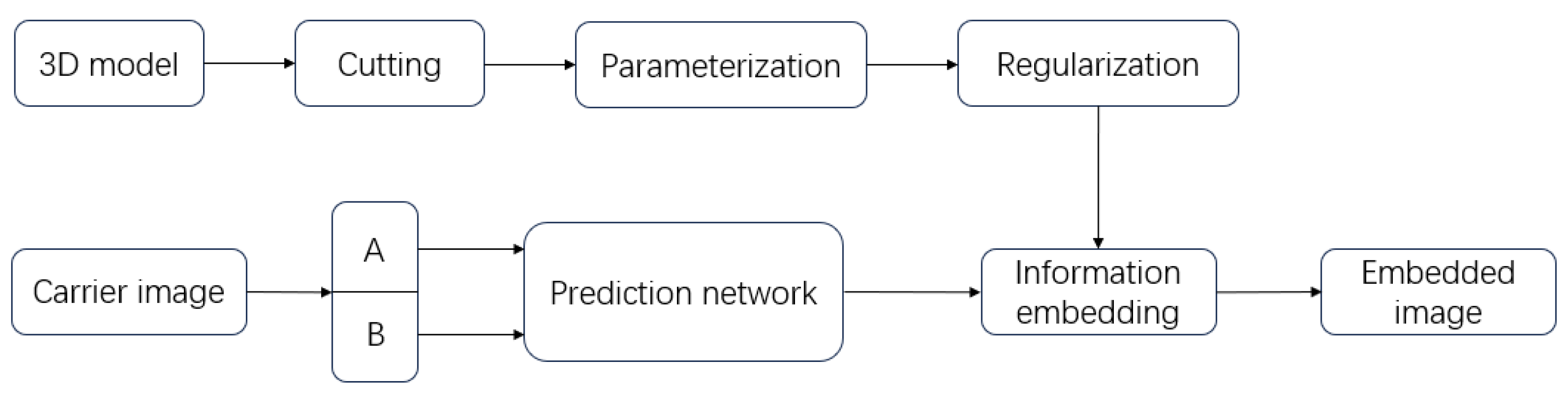
The schematic diagram of the entire project is shown in
Figure 1. We cut, parameterize, and regularize the 3D model to obtain the results for embedding. For the carrier image, we predict it through the proposed convolutional neural network, find points that can embed information, and finally embed the processed 3D model.
The main contributions of this research lie in addressing challenges associated with embedding 3D models into 2D images and increasing the embedding capacity. The presented methods offer innovative insights and avenues for applications in computer graphics and computer vision.
2. Previous Works
The primary objective of reversible data hiding is to preserve the confidentiality of embedded data while maintaining the integrity and reversibility of media data. To accomplish this, reversible data hiding technology typically employs specialized algorithms and techniques. The focus of reversible information hiding technology is mainly on the carrier and confidential information aspects. In this paper, images are used as carriers to conceal confidential information, with three-dimensional geometric data serving as the information to be embedded. Firstly, the development process of reversible data hiding in images, along with significant theories and methods, is discussed. Subsequently, feasible solutions for the regularization research of three-dimensional geometric data are introduced.
2.1. Reversible Data Hiding in Images
In the field of reversible data hiding in 2D images, data hiding is mainly divided into four categories: based on lossless compression, based on numerical transformation, based on error (difference) expansion, and based on histogram shifting. The method based on lossless compression obtains space for data embedding by compressing the original image. For example, Fridrich [
5] proposed a lossless compression encryption method based on bit planes. Then, Fridrich [
6] provided two general methodologies for lossless embedding and offered efficient, simple, and high-capacity methods for three common image format paradigms. Moreover, Celik [
7] presented a new framework for lossless image authentication that offers computational efficiency, public and private key support, and improved tamper localization accuracy. However, these methods usually have low embedding capacity, making it difficult to achieve the hiding of large amounts of data. Furthermore, the image may experience significant distortion after information embedding.
Numerical transformation methods mainly include techniques such as key-based encrypted images and LSB (MSB) replacement. Among them, Yi [
8] proposed a reversible data hiding method in encrypted images using adaptive block level prediction error extension (ABPEE-RDHEI), which encrypts the original image through block arrangement to maintain the spatial redundancy of data embedding and applies stream ciphers to block permutation images to further enhance the security levels. Hong [
9] proposed a method to address the issue of reduced accuracy by better measuring the block smoothness and using side matching schemes to reduce the error rate. Zhang [
10] introduced a separable reversible data hiding scheme for encrypted images; the proposed scheme achieved high embedding capacity and good visual quality of the recovered image. Then, Zhang [
11] introduced a novel method for reversible data hiding within encrypted images; unlike conventional techniques, this approach involves estimating certain pixels prior to encryption, allowing additional data to be concealed within the estimation errors. Yin [
12] proposed a high-capacity RDHEI algorithm based on multi-MSB (most significant bit) prediction and Huffman coding. It adaptively predicts the multi-MSBs of each pixel and marks them in the original image through Huffman coding. The image is encrypted using a stream cipher method, and additional data can be embedded in the available space through multiple MSB replacement. Moreover, Lu [
13] introduced a method of hiding messages using two camouflaged images. Experimental results demonstrate that the method suggested in this study maintains high-quality camouflage images while achieving substantial hiding capacity. Additionally, the quality of the two camouflage images surpasses average standards.
The error (difference) expansion method embeds data by finding errors between adjacent pixels. Tian [
14] first proposed a reversible data hiding method based on difference expansion, which embeds data by expanding the difference between adjacent pixels. Compared with traditional lossless compression methods, the embedding capacity is significantly improved. Li [
15] presented an efficient reversible watermarking technique based on adaptive prediction error expansion and pixel selection. This novel approach integrates two innovative strategies, adaptive embedding and pixel selection, into the PEE process. Furthermore, the adaptive PEE technique facilitates the integration of remarkably large payloads in a single embedding iteration, thus surpassing the capacity limitations of standard PEE. Thodi [
16] introduced a new reversible watermarking algorithm that combines histogram shifting and difference expansion techniques, improving the distortion performance and capacity control. Fallahpour [
17] introduced a novel lossless data hiding technique for digital images using image prediction. The method involves computing prediction errors and subtly altering them through shifting. With the gradual development of error expansion technology, various high-performance predictors have been proposed [
18,
19,
20,
21,
22,
23]. Coltuc [
19] focused on enhancing the embedding quality of prediction error expansion reversible watermarking. Instead of fully embedding the expanded difference into the current pixel, the difference is divided between the current pixel and its prediction context. Jafar [
21] suggested using multiple predictors to enhance embedding capacity without additional overhead. The choice of predictor depends on the prediction error polarity from all predictors. Li [
22] combined the pixel value ordering (PVo) prediction strategy with the prediction error expansion (PEE) technique. It divides the host image into non-overlapping blocks and predicts the maximum and minimum values within each block based on the pixel value orders. Hou [
24] proposed a reversible data hiding scheme that can embed messages in color images without modifying their corresponding grayscale versions. In this algorithm, the unchanged grayscale version is effectively utilized in both the embedding and extraction processes. The information is embedded into the red and blue channels of the color image, and the shift in the grayscale version caused by modifying the red and blue channels is eliminated by adaptively adjusting the green channel, achieving the dual goals of reversibility and grayscale invariance.
The histogram shifting method is a traditional algorithm that embeds data by moving the grayscale histogram. The maximum value of pixel modification is 1, and the algorithm is relatively simple but with low embedding capacity. To solve this problem, Fallahpour [
25] first proposed dividing the image into blocks and applying histogram shifting to embed secret information separately. This method significantly increases the embedding capacity compared to other similar algorithms. Ni [
26] proposed an algorithm that leverages the zero or minimum points in the image histogram and makes slight modifications to pixel grayscale values to embed data. Notably, it can embed more data. Moreover, Tsai [
27] introduced a scheme that employs prediction techniques to explore pixel similarities in the images and utilizes the residual histogram of predicted errors from the host image for data hiding. Furthermore, it leverages the overlap between peak and zero pairs to further enhance the hiding capacity.
2.2. Regularization of Three-Dimensional Geometric Data
Numerous scholars have devised effective techniques to tackle the issue of irregular formats in three-dimensional geometric data. One such method proposed by Qi [
28] is PointNet, which is specifically designed to handle unordered three-dimensional point cloud data. This is achieved through utilizing the coordinates of each point in the three-dimensional space as input parameters for a deep network, which then outputs global features via a max-pooling layer for model classification and segmentation. PointNet is capable of transforming point cloud data into an ordered form by treating them as an unordered set of points and subsequently using a series of transformations and feature extraction operations to convert them into an ordered form. The PointNet architecture comprises two main modules: a transformation network and a feature extraction network. The transformation network facilitates transformations such as rotation and translation on the input point cloud data, rendering it invariant to these transformations. Meanwhile, the feature extraction network can learn the local and global features of the point cloud data and transform them into an ordered form.
Other researchers have employed a different approach by projecting three-dimensional models onto a two-dimensional plane in order to obtain regular results. For instance, Su [
29] obtained two-dimensional images of three-dimensional models from multiple perspectives and fed these images into an MVCNN network to train parameters for model classification. Similarly, Shi [
30] projected three-dimensional models onto the panoramic image of a cylinder. These two methods obtain two-dimensional images of models from multiple perspectives, similar to taking photos of 3D models.
Voxel representation is a method of dividing a three-dimensional space into small, equally sized cubes, each of which contains information about its interior [
31,
32,
33]. A voxel is a three-dimensional extension of the two-dimensional pixel concept, and data based on voxel representation have a regular structure in three-dimensional space, like pixels in two dimensions. However, the disadvantage of using voxel representation is that it requires a lot of storage space to store three-dimensional data, which increases the storage and computation costs. In addition, because the resolution of a voxel representation is fixed, it may be difficult to deal with three-dimensional data with different scales and shapes.
While point-cloud-based techniques have shown success in certain scenarios, they inherently lack geometric topology, which is a crucial feature of three-dimensional geometry. Applications like automatic model generation and model shape retrieval require accurate topological structure information of three-dimensional models. On the other hand, multi-view image methods project three-dimensional models into two-dimensional images, leading to a loss of important geometric and spatial information about the three-dimensional models. Thus, this method cannot be implemented in fields that demand high-quality topological structures of three-dimensional models. Voxel representation, on the other hand, has a limited resolution and consumes a relatively large amount of computing resources. In situations where the network bandwidth is restricted and hardware storage is limited, this data structure is not conducive to data embedding.
3. Area-Preserving Mapping
Area-preserving mapping is achieved via the discrete optimal transportation theory. We use area-preserving mapping and a series of transformations to achieve the regularization of three-dimensional geometric models. This section introduces the relevant theoretical foundations and algorithms.
3.1. Discrete Optimal Transportation Problem
Suppose that we have two subsets in that satisfy the following: (1) is a bounded domain with positive continuous probability measures , and is required to have a convex domain as compact support; (2) is a discrete point set with discrete measure ; (3) the total measures of these two sets are the same.
If a scheme map
satisfies
then
f is called a measure-preserving map. Moreover, the total cost of any scheme map
f can be computed by
where
is the transportation cost function. The discrete OMT problem is to find a map
g with the minimal total cost among all measure-preserving maps.
3.2. Variational Method of the Discrete OMT
If the cost function is defined as
, then the discrete OMT problem can be solved using the following variational method given by Gu et al. [
34].
Given a height vector
, define a convex function as
where
is the dot product of
. The projection of the graph of
induces a power diagram—a polygonal partition of
, where each cell
is the projection of a facet of the graph of
onto
. Meanwhile, the gradient map of the function
on each cell
satisfies
Theorem 1. Suppose that are distinct; there exists a height vector , so that satisfies . Furthermore, h is the maximal point of the convex energy functionand is the OMT map with cost function . From the above theorem, the discrete OMT problem is transformed to define the maximal point of the volume energy . Moreover, because E is convex, the maximum can be computed by Newton’s method efficiently.
The gradient of
is formulated as the following:
Moreover, the Hessian of
is given by
,
where
is the length of the power Delaunay triangulation edge and
is the length of the power diagram edge.
3.3. Algorithm for Semi-Continuous Area-Preserving Mapping
Suppose that the surface
is represented by a discrete triangular mesh
M, and there exists a conformal mapping
from
to planar domain (
; the conformal factor
determines the measure by the formula
. The discrete measure
is defined as follows:
where the summation means to count all the triangles surrounding
.
For the conformal mapping
, we use the normalized Ricci flow algorithm, which preserves the total area of
S [
35]. Newton’s method is used to compute the area-preserving mapping
using the formula of Hessian matrix
. The complete area-preserving mapping is constructed using the composition map
. The whole computational algorithm is described in Algorithm 1.
| Algorithm 1 Area-Preserving Mapping |
- Require:
Mesh M, threshold . - Ensure:
Semi-continuous area-preserving mapping . - 1:
Scale M so that the total area equals . - 2:
Calculate a conformal mapping based on the Ricci flow method. - 3:
Initialize height vector and set target measure on using Equation ( 8). - 4:
Compute the power Voronoi diagram . The area of each cell is denoted as - 5:
Compute the dual power Delaunay triangulation . - 6:
Create Hessian matrix using Equation ( 7). - 7:
Update the height vector with the constraint . - 8:
Repeat steps 4 through 7, until - 9:
Compute the centroid of cell as , map each vertex to .
|
4. Regular Mesh
In the previous step, the triangular mesh of the 3D model was mapped to a two-dimensional parameterization. The mesh in the two-dimensional parameterization domain still appears to be unordered and irregular. We need to rearrange the mesh in the domain so that its mesh connectivity resembles the structure of an image. Thus, we utilize harmonic mapping [
36] to map the two-dimensional parameterization to a square domain, as demonstrated in
Figure 2c. The next step involves employing interpolation techniques to calculate the values of integer points on the square domain, and the details of this process are described in Algorithm 2.
| Algorithm 2 Regular Mesh |
- Require:
Mesh M with square parameterization D, resolution ratio . - Ensure:
Regular mesh r: . - 1:
Scale the parameterization values of points on D to the range of 0–1. - 2:
Adjust the square parameterization D to match the resolution by multiplying the parameterization values of vertices on D by n. - 3:
Identify all integer points’ positions on the parameterization D. These criss-cross integer positions form a grid . - 4:
Determine the triangle in which each integer position point is located and calculate the value at the integer position point by interpolating the three vertices of the corresponding triangle in three-dimensional space. - 5:
Return the grid and its values. .
|
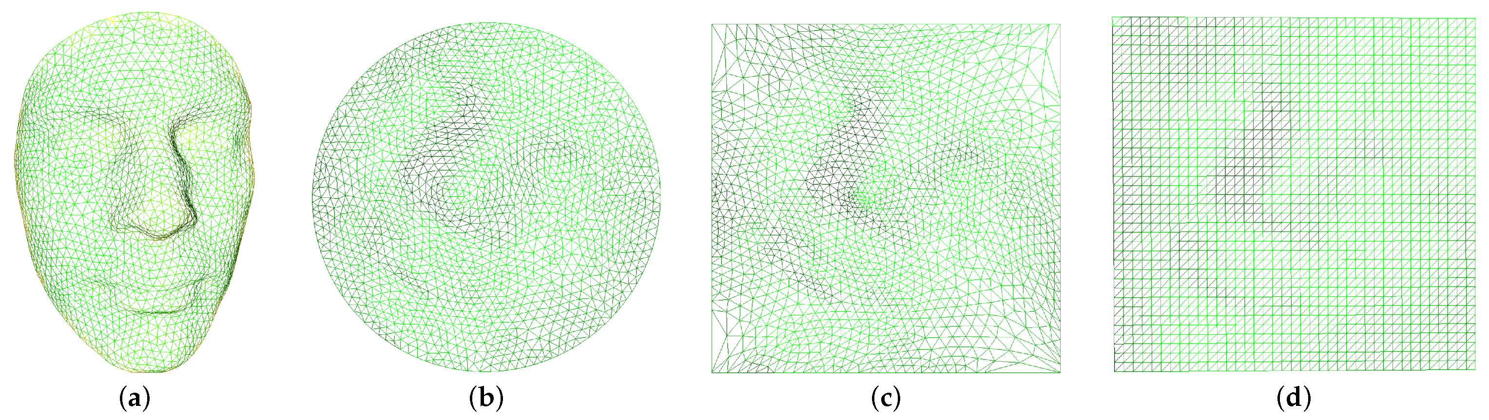
To demonstrate the regularization process of triangular mesh data clearly, we have selected a three-dimensional model with a low resolution.
Figure 2 illustrates the process of regularization of a triangular mesh. The original model is denoted as Alex (a), and the area-preserving mapping obtained by the Alex model using Algorithm 1 is denoted as (b). It can be observed that after the area-preserving mapping, the vertices in the three-dimensional space are mapped to the two-dimensional parameterization to obtain the parameterized result of (a), and the surface area remains unchanged during the mapping process. The result after mapping the boundary of the parameterized result (b) to the boundary of the square is represented as (c), and the regularization result calculated by Algorithm 2 is represented as (d). After a series of mappings, we can fix the disordered triangular mesh data into a regular mesh of the two-dimensional parameter domain, which is similar to the data structure of a two-dimensional image. This data structure will be embedded in the two-dimensional carrier image as secret information in the following calculations.
5. Error Prediction Network and 3D Geometric Data Embedding
In this section, we explore a symmetric method of embedding 3D models into 2D images to ensure reversible information extraction. The primary approach involves using a convolutional neural network to predict the carrier image. Then, the difference between the original carrier image and the predicted one is used to dynamically select pixels for reversible information embedding. As 3D models represented by triangular meshes lack a sequential or regular structure, they need to be regularized. This regularization is accomplished through 2D parameterization. In the regularization process, the three-dimensional geometric model is mapped to the two-dimensional parameterization domain by area-preserving mapping; then, a square boundary and resampling of the two-dimensional parameter domain are performed, and finally the regular structure can be represented by a matrix. Detailed descriptions are given in 3 and 4.
After the 3D geometric model is processed, a regular structure similar to the image is obtained, which has the premise of embedding it into the carrier. Then, we can embed the regularized 3D data into the carrier image like the classic data hiding method. Next, we discuss how to improve the capacity of the carrier.
5.1. Image Pre-Processing
In order to use the proposed convolutional neural network prediction model described in the following text, we partitioned the original carrier image into two subsets of images. To achieve this, we traversed the carrier image
I and set the pixels whose coordinates satisfied Equation (
9) to zero, resulting in the subset image
. Here,
i and
j denote the horizontal and vertical coordinates of the pixel, respectively. We then traversed the image
I again and set the pixels that did not satisfy Equation (
9) to zero, resulting in the subset image
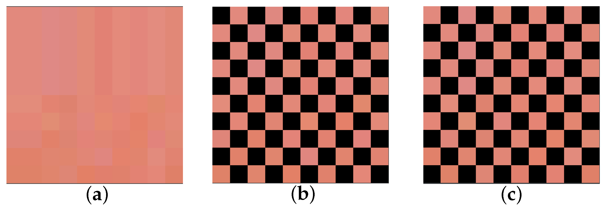
. To illustrate this process, we selected the top-left 100 pixels of Lena for subdivision, as shown in
Figure 3. After subdivision, we obtained two disjoint but highly correlated images. These two subset images are used for convolutional neural network prediction in the following.
5.2. Predictive Convolutional Neural Network
The input of the predictive neural network is an image with a resolution of 512 × 512, with 3 channels, and each channel has a bit depth of 8. The use of 3 channels means that the neural network is processing an RGB image. The purpose of the predictive neural network is to predict two subsets of the same image from each other: through and through . The goal of the network is to train the convolution kernel parameters to minimize the loss of mutual prediction.
Assuming that subset is used to predict subset , the predictive neural network first needs to extract four dimensions of features from . These four dimensions of features correspond to four convolution results, obtained by convolving with 3 × 3, 5 × 5, 7 × 7, and 9 × 9 size convolution kernels, respectively. The features are then fused to predict the pixel values of . While larger convolution kernels can be used to increase the receptive field, they require larger padding values to maintain the same resolution of the predicted output image as the input image. This larger padding value can increase the boundary prediction error, so only the four sizes of convolution kernels mentioned are used for training and prediction.
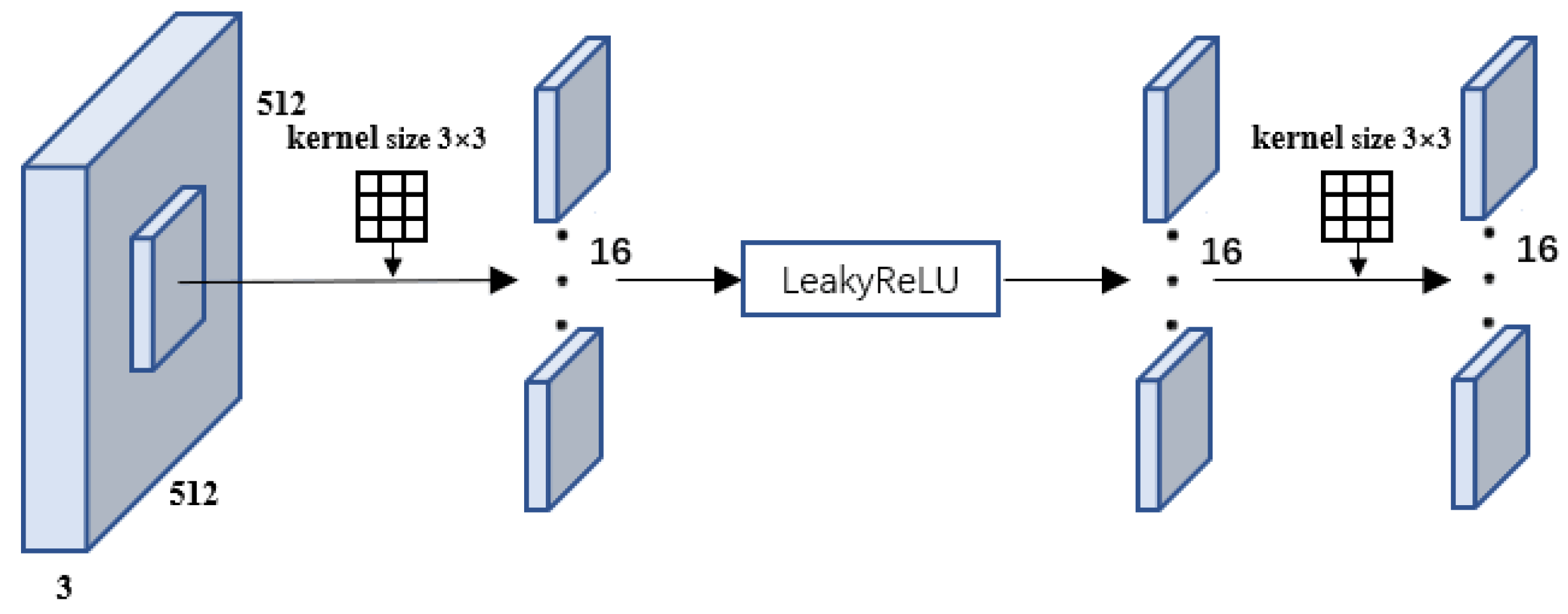
The prediction process is the same for each dimension, and, in this section, we describe the prediction process for the 3 × 3 convolution kernel dimension, as shown in
Figure 4. The input is a 512 × 512 resolution, 3-channel RGB image. Sixteen 3 × 3 × 3 filters are used to convolve the input image, resulting in a feature map with a depth of 8. Appropriate padding is selected during convolution to maintain the resolution of the feature map as the input image. Then, the feature map is passed through a LeakyReLU activation function and finally through a 3 × 3 × 3 size and padding 1 convolution kernel, yielding the feature extraction result.
The process of feature extraction for dimensions other than 3 × 3 is similar, but the kernel size needs to be adjusted accordingly. For instance, the feature extraction process for the 5 × 5 convolutional dimension requires sixteen 5 × 5 × 3 filters to convolve the input image. The feature extraction process for other dimensions involves capturing the relationship between the predicted pixel value and the surrounding pixel values within different ranges.
5.3. Optimizing Parameters of Predictive Convolutional Neural Networks
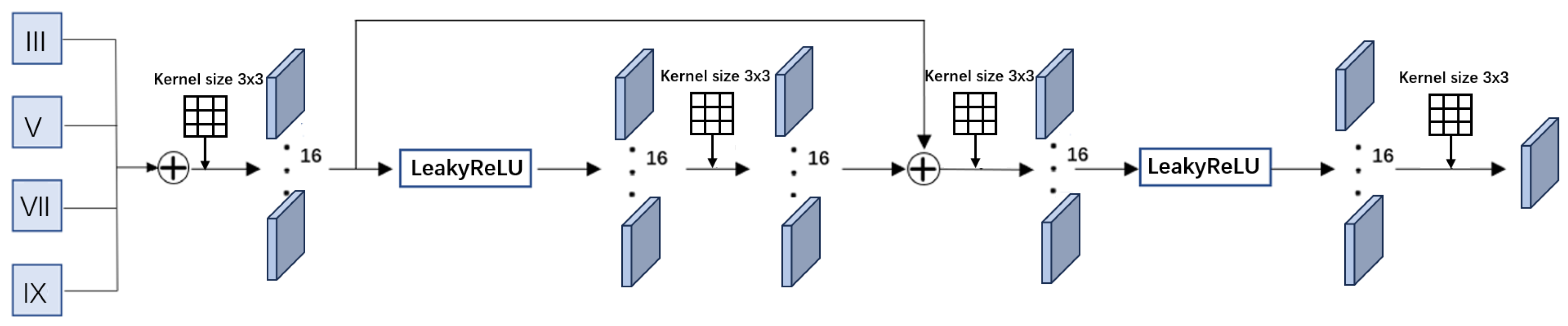
The original carrier images are processed through a predictive neural network to obtain predictions in four dimensions. These predictions are then superimposed to obtain the final prediction value, as shown in
Figure 5. The purpose of this process is to merge the feature maps obtained from the four dimensions. To achieve this, the feature maps from each dimension are first added together, and the resulting sum undergoes a convolution operation similar to the feature extraction process in each dimension. The output of this operation is then added to the feature maps of the four dimensions and convolved to obtain an output image consistent with the original image resolution. This output image is the predicted image
.
The difference between the predicted image
and the real image
is referred to as the loss value. To train the prediction network and minimize the prediction error, backpropagation [
37] and the Adam optimizer [
38] are utilized to minimize the following loss function:
Here, N represents the number of training data, is the weight decay, and represents the weights of the convolutional neural network. To prevent overfitting, a regularization term is added.
During the parameter training process, 2000 color images with a size of 512 × 512 pixels were selected to train the model. The subset image was then input into the trained network to extract features and predict the final image . In order to achieve reversible information extraction, we utilized the subset image embedded with information to generate the predicted image .
5.4. Error-Adaptive Embedding
Assuming that the confidential information is embedded in the subset image , the error value sequence obtained by subtracting the generated subset prediction image from the original subset image is used for the subsequent selection of embedding coordinates and channels.
Each vertex of the original 3D model data is represented by floating point numbers. In order to improve the accuracy of the model and match the pixel values of the carrier image, the vertex coordinates of the 3D model are normalized to be between 0 and 65,535.
Due to the large normalized values of the 3D model, in order to ensure that the pixel values of the carrier image do not overflow after embedding the 3D model into the carrier image, and to ensure that the embedded model can still obtain acceptable visual quality, we treat the coordinate information of the 3D model as a five-digit number and divide it into five single digits. For example, if the coordinate information of a certain point is 5963, the resulting numbers after segmentation are 0, 5, 9, 6, and 3. We concatenate all segmented single digits to obtain the secret information sequence Q.
The threshold
K is dynamically selected based on the number of model vertices to be embedded. Firstly, set
, and then iterate through the sequence
to count the number of absolute values that are less than or equal to
K. If it satisfies Formula (
11), increment the value of
K by 1. Otherwise, the current threshold
K is recorded.
Then, use Formula (
12) to embed
into the carrier image, where
represents the pixel values of the original subset image
, resulting in the embedded image
. Next, use the image
to predict and generate image
, and repeat the above embedding process to obtain image
. Finally, concatenate images
and
to obtain image
, which contains the secret information.
5.5. Extraction of Information and Reconstruction of 3D Models
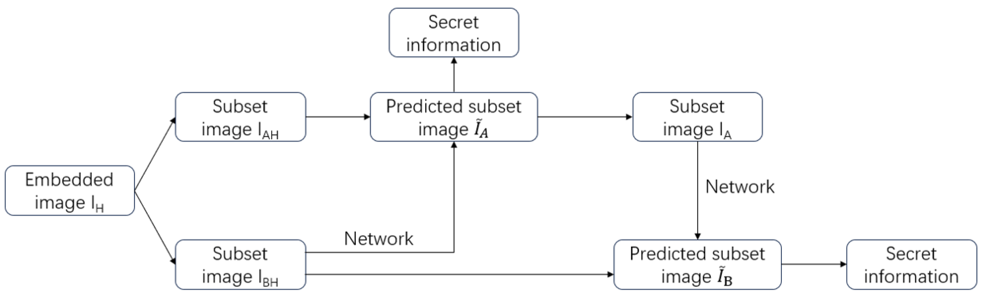
Due to the symmetry of the algorithm proposed earlier, the extraction of information and reconstruction of 3D models can be considered the inverse process of the algorithm described above. The process of extracting information is shown in
Figure 6. Firstly, the subset image
containing secret information is subjected to the aforementioned neural network prediction to obtain the predicted subset image
. Decrypting the compared images
and
can reveal some of the secret information and subset image
. Applying the same process to image
can reveal the hidden secret information in image
. A complete set can be obtained by combining
and
. This set consists of data with the same resolution as the original 3D model, but in a two-dimensional parameterization. It comprises three channels, each representing one of the three vertex coordinates of the 3D model in space. Since the regularization process of the three-dimensional model is reversible, the three-dimensional point coordinates can be recovered from the two-dimensional parameter field values. Then, by parameterizing and inversely processing, the original 3D model can be obtained.
6. Experimental Results
In this section, we discuss the performance of the proposed method in terms of the embedded capacity and visual quality compared to other methods. The experiment was conducted using PyCharm 2022 and MATLAB R2021b on a Windows 10 laptop with an Intel Core i7-10750H CPU and NVIDIA RTX 2060 GPU.
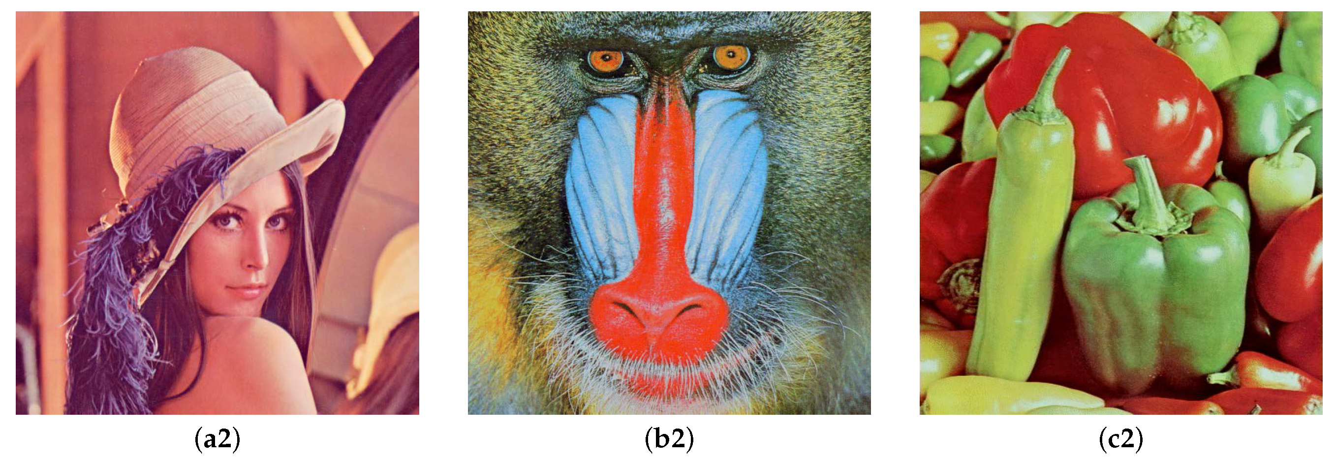
We embedded three-dimensional models of Luke, Sophia, and Bunny into 8-bit depth color images of Lena, Baboon, and Peppers, respectively, all of which were of size 512 × 512. Since our proposed method maps three-dimensional models of varying resolutions to a two-dimensional parameterization and then regularizes them, we used the regularized data for our experiment. After regularization, the three-dimensional model possesses identical dimensions and resolution. The two-dimensional images and three-dimensional models used in the experiment are displayed in
Figure 7 and
Figure 8, respectively.
Table 1 shows the vertex, triangle numbers, and regularized uniform sizes of the three-dimensional models.
When embedding data, the three-dimensional model is transformed into a regularized ordered array, forming a row and column structure similar to that of an image. The values are then embedded successively into the two-dimensional image according to the row and column sequence.
Figure 2 displays both the three-dimensional model and its corresponding regularization results.
6.1. Performance
The calculation formula for PSNR is shown in Formula (
13), where
N represents the depth of the image, MSE is the mean square error between the original image and the processed image, and the formula is Formula (
14), where
m and
n represent the width and height of the image, and
and
represent the pixel points of the image
i row and
j column before and after embedding information.
The proposed algorithm was then used to embed the model into the image in a reversible manner. Due to the large amount of information in the 3D model, it is not possible to fully embed it through a two-dimensional image. Therefore, we divided the information that needed to be embedded into two equal lengths and used two identical images to embed the 3D model. The threshold and average PSNR of these two images are shown in
Table 2 (8-bit color image as carrier).
To further illustrate the performance of the proposed algorithm, we compared it with the algorithms proposed by Fallahpour [
25], Li [
15], Yin [
12], and Hou [
24]. Since these algorithms embed random bit sequences, we also converted the three-dimensional model into a bit sequence, the length of which is shown in
Table 3.
It should be noted that Fallahpour, Li, and Yin’s algorithms are designed for information hiding in grayscale images. Therefore, to achieve a fair comparison, all the color images that they used in their experiments were converted to grayscale. This can be done in various ways [
39,
40,
41], and we selected Formula (
15), which takes into account the sensitivity of the human eye to different colors, and then the results were calculated by relevant methods for comparison.
where
is the converted grayscale pixel value, and ⌊
x⌉ denotes the nearest integer to
x.
The proposed method uses 8-bit grayscale images as carriers to embed the model, requiring six identical images. The threshold and PSNR for the use of 8-bit grayscale images are shown in
Table 4.
6.2. Embedded Capacity
In this section, we discuss the embedding capacities of different algorithms. Existing algorithms are unable to embed a large amount of data in a single image. Therefore, we analyze how many images are required to embed the bit sequence, the amount of data that can be embedded in each image, and the total number of images required to embed, as shown in
Table 5. According to the data presented in the table, our method requires six grayscale images as carriers for the embedding of Luke, Sophia, or Bunny. Among the several methods compared, our method and Yin’s method have the highest embedding capacity. Yin requires five or six Lena and Peppers images to embed the model, while using Baboon as the carrier requires 11 images. Compared to our algorithm, no matter which image is chosen as the carrier, six images are required. The two methods have similar embedding capacity, and, in some examples, our method outperforms Yin’s method in terms of embedding capacity. Fallahpour’s method has a low embedding volume, requiring 596 Lena images to embed one Bunny model. Li’s method and Hou’s method fall somewhere in between the three mentioned earlier: 10 and 39 Lena images are required, respectively, to embed one Bunny model.
Fallahpour’s algorithm uses histogram shifting to embed information only at peak points. However, due to the limitation of the number of peak points, even if the image is divided into four parts, each part having a peak point for data embedding, the effect is still far from satisfactory. Li used adaptive prediction error expansion and pixel selection algorithms. At high embedding rates, the visual quality is poor (PSNR < 30). Therefore, we only compare the embedding capacity when the PSNR is greater than 30. Yin used multi-MSB prediction and Huffman coding algorithms to achieve high embedding performance by embedding multiple bits of information in a pixel. Hou embedded secret information into triplets, effectively increasing the amount of information embedded.
Compared with the algorithms proposed by Fallahpour, Li, Yin, and Hou, our proposed algorithm is one of the best in terms of embedded capacity.
6.3. Time Complexity
To further explain the embedding performance of the algorithm proposed in the article, we use time complexity to measure the embedding efficiency of the program.
The algorithm proposed in the article uses the traversal of the image to find points that meet the threshold for embedding information during the embedding process, resulting in a time complexity of . The algorithm proposed by Fallahpour is relatively simple, embedding images in peak points through traversal, with a time complexity of 2. Li’s method traverses the image twice, searching for error points that can be embedded and embedding them separately, resulting in a time complexity of 2. Hou embedding requires the modification of the selected pixels and adjustment of the g-channel based on the embedded message. This step involves traversing and calculating pixels, with a time complexity of . Yin’s method needs to traverse the image during embedding and hide information based on Huffman encoding and auxiliary information. Due to the time complexity of the Huffman encoding used being , the embedding time complexity is .
The algorithm proposed in the article has the same time complexity as most information embedding algorithms.
6.4. Visual Quality
In this section, we utilize the PSNR value and differential image to represent the image’s visual quality after data embedding.
6.4.1. PSNR Value
Table 6 presents a comparison of the four previously mentioned algorithms with the algorithm proposed in this paper. Fallahpour’s method has a high PSNR value because of its low embedding capacity. Li’s approach needs to balance the embedding capacity and visual quality, and it cannot maintain a high PSNR at high embedding rates. Yin used traditional cryptographic methods to rearrange the pixels of the image, resulting in significant differences between the images before and after embedding, resulting in a lower PSNR value. Hou’s method indirectly improves the PSNR value of the image by introducing triplets and adjusting the corresponding RGB values to ensure the invariance of the image’s grayscale. While the embedding capacity of our method is much higher than that of Fallahpour, Li, and Hou’s methods, the PSNR performance calculated by our method is better than that of Li’s method, and the effect is similar to that of Hou’s method. Our method exhibits a higher PSNR value when the embedding amount is similar to that in Yin’s method.
Figure 9 displays a comparison of the original images and carried images that embed the Bunny model using the algorithm presented in this paper. Upon observing the original image and the encrypted image, it is found that there is no significant difference between the two, and their visual effects are very similar. Therefore, the algorithm proposed in this article can maintain acceptable image quality.
6.4.2. Differential Image
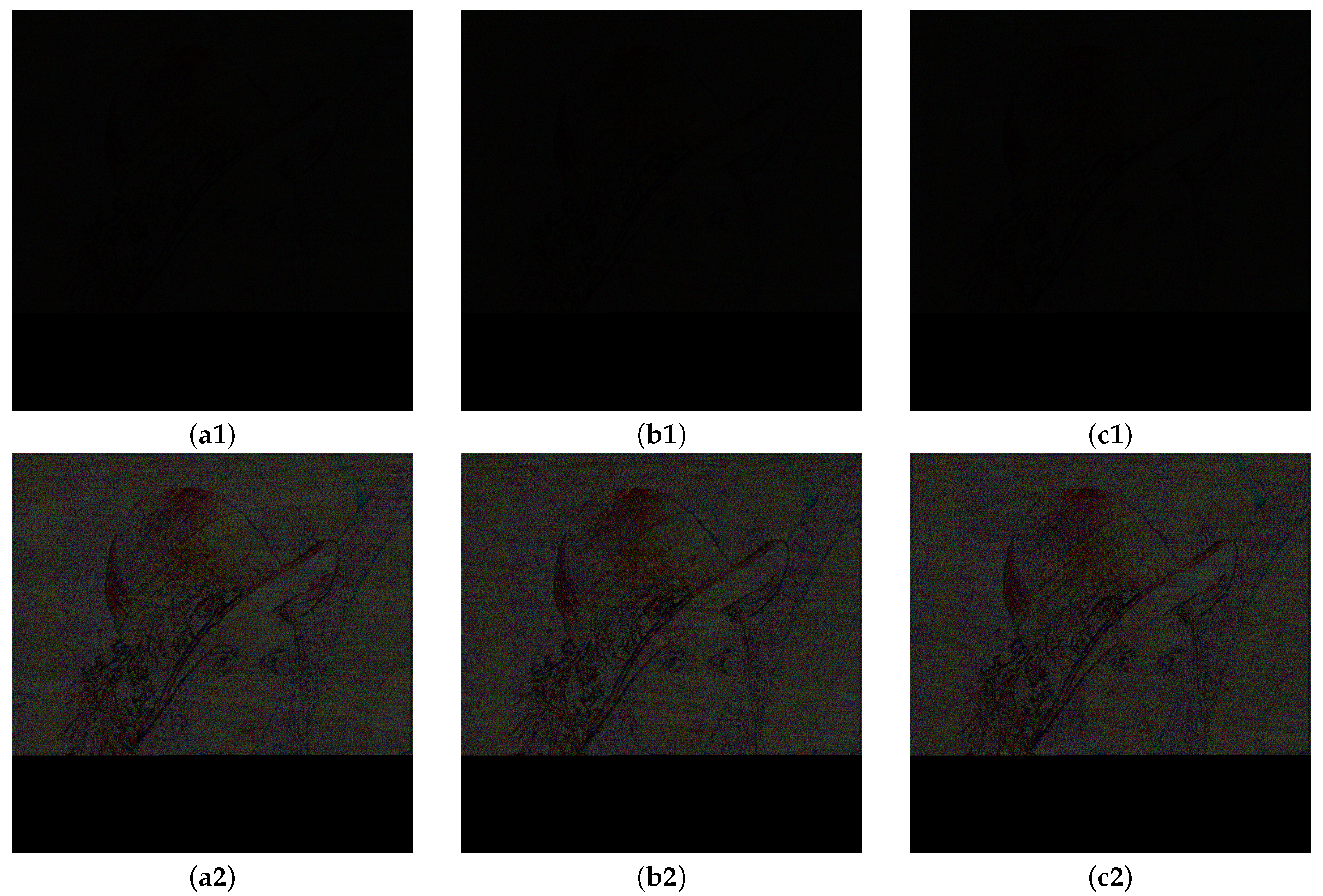
The differential image obtained by subtracting the carrier images before and after embedding the information is shown in
Figure 10.
Figure 10(a1),
Figure 10(b1), and
Figure 10(c1), represent embedding Luke, Sophia, and Bunny models into Lena images, respectively. Due to the maximum change in the pixel points of the algorithm proposed in the article being 9, when viewed from the perspective of the differential images, there will be no significant visual differences between the images before and after embedding information. Therefore, we multiply each pixel in the differential image by 10 to visually observe the embedding of information.
Figure 10(a2),
Figure 10(b2), and
Figure 10(c2), respectively, show the results of multiplying the pixel points in
Figure 10(a1),
Figure 10(b1), and
Figure 10(c1) by 10.
6.4.3. Discussion
The experimental results indicate that the algorithm proposed in this paper significantly enhances the data embedding capacity of the carrier image while maintaining acceptable visual quality even at high embedding capacities.
7. Conclusions
This paper presents a technique for the embedding of 3D models into 2D images in a reversible manner. An adaptive convolutional neural network is utilized to process the carrier image, enabling the prediction of errors and identification of suitable points for the embedding of information. The 3D model is represented by a triangle mesh, which is parametrized and regularized for reversible embedding in the image.
The main contribution of this paper is to embed the disordered triangular mesh data after regularization into the image with the prediction error obtained by a convolutional neural network. The error can be adapted during the embedding process, and the obtained reversible 3D data hiding method has high embedding capacity. Compared to other methods, the proposed approach enhances the embedding capacity with acceptable visual quality. The proposed method can be widely used in fields such as digital medicine, virtual reality, computer-aided design, and so on. It can protect data privacy and verify the rights of 3D digital products. However, there are certain limitations to this method. Handling models with a genus greater than 1 requires additional processing of the 3D model, which will be the focus of future research.
Author Contributions
Conceptualization, G.H. and K.Q.; methodology, Y.L.; software, H.L.; validation, X.X., H.X. and G.H.; formal analysis, K.Q.; investigation, Y.L.; resources, H.L.; data curation, X.X.; writing—original draft preparation, H.X.; writing—review and editing, G.H.; visualization, K.Q.; supervision, Y.L.; project administration, H.L.; funding acquisition, X.X. All authors have read and agreed to the published version of the manuscript.
Funding
This work was supported by the National Natural Science Foundation of China (Project Number: 62362064, 62166045, 62161051), the Yunnan Fundamental Research Projects (Project Number: 202201AT070166), and the Scientific Research Foundation of Yunnan Provincial Department of Education (Project Number: 2022J0475).
Institutional Review Board Statement
Not applicable.
Informed Consent Statement
Not applicable.
Data Availability Statement
All the relevant data are included within the paper.
Conflicts of Interest
The authors declare no conflict of interest.
References
- Onyshchenko, S.; Yanko, A.; Hlushko, A.; Sivitska, S. Increasing information protection in the information security management system of the enterprise. In Proceedings of the International Conference Building Innovations, Baku, Poltava, 1–2 June 2020; pp. 725–738. [Google Scholar]
- Jiang, R.; Han, S.; Zhang, Y.; Chen, T.; Song, J. Medical big data access control model based on UPHFPR and evolutionary game. Alex. Eng. J. 2022, 61, 10659–10675. [Google Scholar] [CrossRef]
- Jiang, R.; Xin, Y.; Chen, Z.; Zhang, Y. A medical big data access control model based on fuzzy trust prediction and regression analysis. Appl. Soft Comput. 2022, 117, 108423. [Google Scholar] [CrossRef]
- Jiang, R.; Kang, Y.; Liu, Y.; Liang, Z.; Duan, Y.; Sun, Y.; Liu, J. A trust transitivity model of small and medium-sized manufacturing enterprises under blockchain-based supply chain finance. Int. J. Prod. Econ. 2022, 247, 108469. [Google Scholar] [CrossRef]
- Fridrich, J.; Goljan, M.; Du, R. Invertible authentication. In Proceedings of the Security and Watermarking of Multimedia Contents III, SPIE, Las Vegas, NV, USA, 2–4 April 2001; Volume 4314, pp. 197–208. [Google Scholar]
- Fridrich, J.; Goljan, M.; Du, R. Lossless data embedding for all image formats. In Proceedings of the Security and Watermarking of Multimedia Contents IV, SPIE, San Jose, CA, USA, 29 April 2002; Volume 4675, pp. 572–583. [Google Scholar]
- Celik, M.U.; Sharma, G.; Tekalp, A.M. Lossless watermarking for image authentication: A new framework and an implementation. IEEE Trans. Image Process. 2006, 15, 1042–1049. [Google Scholar] [CrossRef] [PubMed]
- Yi, S.; Zhou, Y.; Hua, Z. Reversible data hiding in encrypted images using adaptive block-level prediction-error expansion. Signal Process. Image Commun. 2018, 64, 78–88. [Google Scholar] [CrossRef]
- Hong, W.; Chen, T.S.; Wu, H.Y. An improved reversible data hiding in encrypted images using side match. IEEE Signal Process. Lett. 2012, 19, 199–202. [Google Scholar] [CrossRef]
- Zhang, X. Separable reversible data hiding in encrypted image. IEEE Trans. Inf. Forensics Secur. 2011, 7, 826–832. [Google Scholar] [CrossRef]
- Zhang, W.; Ma, K.; Yu, N. Reversibility improved data hiding in encrypted images. Signal Process. 2014, 94, 118–127. [Google Scholar] [CrossRef]
- Yin, Z.; Xiang, Y.; Zhang, X. Reversible data hiding in encrypted images based on multi-MSB prediction and Huffman coding. IEEE Trans. Multimed. 2019, 22, 874–884. [Google Scholar] [CrossRef]
- Lu, T.C.; Tseng, C.Y.; Wu, J.H. Dual imaging-based reversible hiding technique using LSB matching. Signal Process. 2015, 108, 77–89. [Google Scholar] [CrossRef]
- Tian, J. Reversible data embedding using a difference expansion. IEEE Trans. Circuits Syst. Video Technol. 2003, 13, 890–896. [Google Scholar] [CrossRef]
- Li, X.; Yang, B.; Zeng, T. Efficient reversible watermarking based on adaptive prediction-error expansion and pixel selection. IEEE Trans. Image Process. 2011, 20, 3524–3533. [Google Scholar] [PubMed]
- Thodi, D.M.; Rodríguez, J.J. Expansion embedding techniques for reversible watermarking. IEEE Trans. Image Process. 2007, 16, 721–730. [Google Scholar] [CrossRef]
- Fallahpour, M. Reversible image data hiding based on gradient adjusted prediction. IEICE Electron. Express 2008, 5, 870–876. [Google Scholar] [CrossRef]
- Hu, R.; Xiang, S. CNN prediction based reversible data hiding. IEEE Signal Process. Lett. 2021, 28, 464–468. [Google Scholar] [CrossRef]
- Coltuc, D. Improved embedding for prediction-based reversible watermarking. IEEE Trans. Inf. Forensics Secur. 2011, 6, 873–882. [Google Scholar] [CrossRef]
- Coltuc, D. Low distortion transform for reversible watermarking. IEEE Trans. Image Process. 2011, 21, 412–417. [Google Scholar] [CrossRef] [PubMed]
- Jafar, I.F.; Darabkh, K.A.; Al-Zubi, R.T.; Al Na’mneh, R.A. Efficient reversible data hiding using multiple predictors. Comput. J. 2016, 59, 423–438. [Google Scholar] [CrossRef]
- Li, X.; Li, J.; Li, B.; Yang, B. High-fidelity reversible data hiding scheme based on pixel-value-ordering and prediction-error expansion. Signal Process. 2013, 93, 198–205. [Google Scholar] [CrossRef]
- Sachnev, V.; Kim, H.J.; Nam, J.; Suresh, S.; Shi, Y.Q. Reversible watermarking algorithm using sorting and prediction. IEEE Trans. Circuits Syst. Video Technol. 2009, 19, 989–999. [Google Scholar] [CrossRef]
- Hou, D.; Zhang, W.; Chen, K.; Lin, S.J.; Yu, N. Reversible data hiding in color image with grayscale invariance. IEEE Trans. Circuits Syst. Video Technol. 2018, 29, 363–374. [Google Scholar] [CrossRef]
- Fallahpour, M. High capacity lossless data hiding based on histogram modification. IEICE Electron. Express 2007, 4, 205–210. [Google Scholar] [CrossRef]
- Ni, Z.; Shi, Y.Q.; Ansari, N.; Su, W. Reversible data hiding. IEEE Trans. Circuits Syst. Video Technol. 2006, 16, 354–362. [Google Scholar]
- Tsai, P.; Hu, Y.C.; Yeh, H.L. Reversible image hiding scheme using predictive coding and histogram shifting. Signal Process. 2009, 89, 1129–1143. [Google Scholar] [CrossRef]
- Qi, C.R.; Su, H.; Mo, K.; Guibas, L.J. Pointnet: Deep learning on point sets for 3D classification and segmentation. In Proceedings of the IEEE Conference on Computer Vision and Pattern Recognition, Honolulu, HI, USA, 21–26 July 2017; pp. 652–660. [Google Scholar]
- Su, H.; Maji, S.; Kalogerakis, E.; Learned-Miller, E. Multi-view convolutional neural networks for 3D shape recognition. In Proceedings of the IEEE International Conference on Computer Vision, Santiago, Chile, 7–13 December 2015; pp. 945–953. [Google Scholar]
- Shi, B.; Bai, S.; Zhou, Z.; Bai, X. Deeppano: Deep panoramic representation for 3-D shape recognition. IEEE Signal Process. Lett. 2015, 22, 2339–2343. [Google Scholar] [CrossRef]
- Laine, S.; Karras, T. Efficient sparse voxel octrees. In Proceedings of the 2010 ACM SIGGRAPH Symposium on Interactive 3D Graphics and Games, Washington, DC, USA, 19 February 2010; pp. 55–63. [Google Scholar]
- Baert, J.; Lagae, A.; Dutré, P. Out-of-core construction of sparse voxel octrees. In Proceedings of the 5th High-Performance Graphics Conference, Anaheim, CA, USA, 19 July 2013; pp. 27–32. [Google Scholar]
- Nießner, M.; Zollhöfer, M.; Izadi, S.; Stamminger, M. Real-time 3D reconstruction at scale using voxel hashing. ACM Trans. Graph. (ToG) 2013, 32, 1–11. [Google Scholar] [CrossRef]
- Gu, X.; Luo, F.; Sun, J.; Yau, S.T. Variational principles for Minkowski type problems, discrete optimal transport, and discrete Monge-Ampere equations. AJM 2016, 20, 383–398. [Google Scholar] [CrossRef]
- Jin, M.; Kim, J.; Luo, F.; Gu, X. Discrete surface Ricci flow. IEEE Trans. Vis. Comput. Graph. 2008, 14, 1030–1043. [Google Scholar] [CrossRef] [PubMed]
- Wei, X.; Li, H.; Gu, X.D. Three Dimensional Face Recognition via Surface Harmonic Mapping and Deep Learning. In Proceedings of the Biometric Recognition: 12th Chinese Conference, CCBR 2017, Shenzhen, China, 28–29 October 2017; pp. 66–76. [Google Scholar]
- LeCun, Y.; Bottou, L.; Bengio, Y.; Haffner, P. Gradient-based learning applied to document recognition. Proc. IEEE 1998, 86, 2278–2324. [Google Scholar] [CrossRef]
- Kingma, D.P.; Ba, J. Adam: A method for stochastic optimization. arXiv 2014, arXiv:1412.6980. [Google Scholar]
- Gooch, A.A.; Olsen, S.C.; Tumblin, J.; Gooch, B. Color2gray: Salience-preserving color removal. ACM Trans. Graph. (TOG) 2005, 24, 634–639. [Google Scholar] [CrossRef]
- Grundland, M.; Dodgson, N.A. Decolorize: Fast, contrast enhancing, color to grayscale conversion. Pattern Recognit. 2007, 40, 2891–2896. [Google Scholar] [CrossRef]
- Sowmya, V.; Govind, D.; Soman, K. Significance of incorporating chrominance information for effective color-to-grayscale image conversion. Signal Image Video Process. 2017, 11, 129–136. [Google Scholar] [CrossRef]
Figure 1.
The process of the proposed algorithm.
Figure 1.
The process of the proposed algorithm.
Figure 2.
Regularization of triangular mesh. (a) shows the Alex model, (b) displays the area-preserving mapping result of the Alex model, (c) exhibits the square boundary parameterization, and (d) demonstrates the regularized result.
Figure 2.
Regularization of triangular mesh. (a) shows the Alex model, (b) displays the area-preserving mapping result of the Alex model, (c) exhibits the square boundary parameterization, and (d) demonstrates the regularized result.
Figure 3.
Original image and two subset images. (a) is the carrier image I, (b) is the subset image , and (c) is the subset image .
Figure 3.
Original image and two subset images. (a) is the carrier image I, (b) is the subset image , and (c) is the subset image .
Figure 4.
The 3 × 3 dimension feature extraction process.
Figure 4.
The 3 × 3 dimension feature extraction process.
Figure 5.
Image prediction process. III represents the prediction feature map obtained from a 3 × 3 dimension, V represents the prediction feature map obtained from a 5 × 5 dimension, VII represents the prediction feature map obtained from a 7 × 7 dimension, and IX represents the prediction feature map obtained from a 9 × 9 dimension. These feature maps are added together and then undergo a series of convolutional operations to generate the final prediction.
Figure 6.
The process of extracting information.
Figure 6.
The process of extracting information.
Figure 7.
Images used in the experiment. (a) is Lena, (b) is Baboon, and (c) is Peppers.
Figure 7.
Images used in the experiment. (a) is Lena, (b) is Baboon, and (c) is Peppers.
Figure 8.
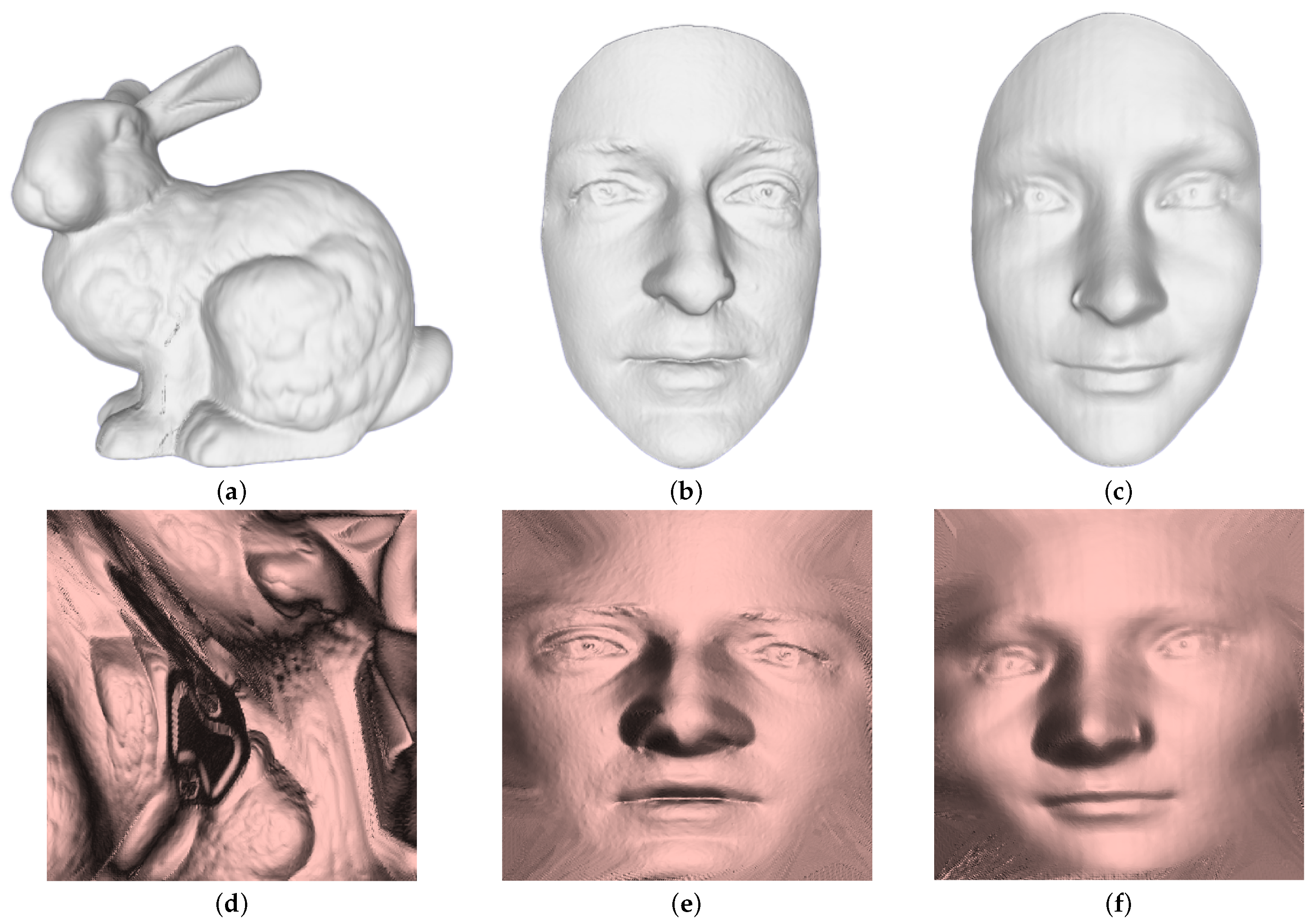
The experiment utilized three-dimensional models, namely the Bunny model (a), Luke model (b), and Sophia model (c). Their respective regularization results are labeled as (d) for the Bunny model, (e) for the Luke model, and (f) for the Sophia model.
Figure 8.
The experiment utilized three-dimensional models, namely the Bunny model (a), Luke model (b), and Sophia model (c). Their respective regularization results are labeled as (d) for the Bunny model, (e) for the Luke model, and (f) for the Sophia model.
Figure 9.
Comparison of original image and carried image. (a1,b1,c1) are the original images. (a2,b2,c2) are the carried images after embedding the Bunny model into the original images.
Figure 9.
Comparison of original image and carried image. (a1,b1,c1) are the original images. (a2,b2,c2) are the carried images after embedding the Bunny model into the original images.
Figure 10.
Differential images of embedding Luke, Sophia, and Bunny models into Lena images. (a1) represents the differential image of the difference before and after embedding Luke model into Lena image, (b1) represents the differential image of the difference before and after embedding Sophia model into Lena image, (c1) represents the differential image of the difference before and after embedding Bunny model into Lena image. (a2,b2,c2) represent the images obtained by multiplying the pixel values of (a1,b1,c1) by 10, respectively.
Table 1.
The number of vertices and triangles of the experimental models.
Table 1.
The number of vertices and triangles of the experimental models.
| Model | Number of Vertices | Number of Faces | Unified Vertices | Unified Triangles |
|---|
| Bunny | 35,947 | 69,451 | | |
| Luke | 21,371 | 42,281 | 65,536 | 129,540 |
| Sophia | 21,043 | 41,587 | | |
Table 2.
Performance of the proposed model (8-bit color image as carrier).
Table 2.
Performance of the proposed model (8-bit color image as carrier).
| | Hidden Model |
|---|
| Carrier | Luke | Sophia | Bunny |
|---|
| | Threshold | PSNR | Threshold | PSNR | Threshold | PSNR |
|---|
| Lena | 5 | 36.19 | 5 | 36.4 | 5 | 36.27 |
| Baboon | 17 | 36.34 | 17 | 36.39 | 17 | 36.36 |
| Peppers | 8 | 36.19 | 8 | 36.37 | 8 | 36.28 |
Table 3.
Lengths of different model bit sequences.
Table 3.
Lengths of different model bit sequences.
| Embedded Model | Bit Sequence Length |
|---|
| Luke | 3,012,351 |
| Sophia | 3,015,333 |
| Bunny | 2,927,157 |
Table 4.
Performance of the proposed model (8-bit grayscale image as carrier).
Table 4.
Performance of the proposed model (8-bit grayscale image as carrier).
| | Hidden Model |
|---|
| Carrier | Luke | Sophia | Bunny |
|---|
| | Threshold | PSNR | Threshold | PSNR | Threshold | PSNR |
|---|
| Lena | 6 | 36.06 | 6 | 36.52 | 6 | 36.16 |
| Baboon | 17 | 36.04 | 17 | 36.53 | 17 | 36.19 |
| Peppers | 7 | 36.06 | 7 | 36.54 | 7 | 36.12 |
Table 5.
Fallahpour, Li, Yin and Hou’s methods in terms of embedded capacity.
Table 5.
Fallahpour, Li, Yin and Hou’s methods in terms of embedded capacity.
| Method | Carrier | Embedable Amount
per Image | Number of Images |
|---|
| Luke | Sophia | Bunny |
|---|
| | Lena | 4912 | 614 | 614 | 596 |
| Fallahpour | Baboon | 8662 | 348 | 349 | 338 |
| | Peppers | 24,301 | 124 | 125 | 121 |
| | Lena | 300,000 | 11 | 11 | 10 |
| Li | Baboon | 130,000 | 24 | 24 | 23 |
| | Peppers | 200,000 | 16 | 16 | 15 |
| | Lena | 677,212 | 5 | 5 | 5 |
| Yin | Baboon | 279,391 | 11 | 11 | 11 |
| | Peppers | 602,714 | 5 | 6 | 5 |
| | Lena | 101,920 | 30 | 30 | 39 |
| Hou | Baboon | 182,000 | 17 | 17 | 17 |
| | Peppers | 211,120 | 15 | 15 | 14 |
Table 6.
Proposed, Fallahpour, Li, Yin and Hou’s methods in terms of visual quality.
Table 6.
Proposed, Fallahpour, Li, Yin and Hou’s methods in terms of visual quality.
| | Average PSNR (dB) |
|---|
| | Proposed Method | Fallahpour | Li | Yin | Hou |
|---|
| Lena | 36.24 | 50.9 | 32.54 | 7.79 | 40.21 |
| Baboon | 36.25 | 52.05 | 33.38 | 7.63 | 37.45 |
| Peppers | 36.24 | 60.23 | 32.75 | 7.56 | 36.99 |
| Disclaimer/Publisher’s Note: The statements, opinions and data contained in all publications are solely those of the individual author(s) and contributor(s) and not of MDPI and/or the editor(s). MDPI and/or the editor(s) disclaim responsibility for any injury to people or property resulting from any ideas, methods, instructions or products referred to in the content. |
© 2023 by the authors. Licensee MDPI, Basel, Switzerland. This article is an open access article distributed under the terms and conditions of the Creative Commons Attribution (CC BY) license (https://creativecommons.org/licenses/by/4.0/).


