1. Introduction
Product optimization design (or optimal product design, OPD) refers to the optimization of product recommendation, market share, and product line configuration by collecting user preference information for product concepts [
1]. This problem is prevalent in various domains, including product design [
2,
3], the supply chain [
4], and personalized recommendations [
5]. Among these, the collection of user preference information is a key factor in solving this problem and has a direct influence on the optimization results. Employing interactive techniques to collect user preference information is the most direct and widespread method. However, facing an extensive space solution, excessive interaction can lead to user fatigue. Therefore, how to help users quickly find satisfactory solutions in a vast sea of information has become the focus of much research.
The evolutionary algorithm-based Top-N algorithm is a representative approach for solving this problem [
6]. The distinguishing feature of such algorithms is that users only need to evaluate N-out-of-M individuals in the population, while the remaining individuals are evaluated using surrogate models. The most commonly used surrogate models include polynomial regression [
7], support vector machines [
8], radial basis function (RBF) [
9], neural networks [
10], Kriging [
11,
12], and so on. These surrogate models are all statistical methods, and their learning and predictive performance are highly dependent on the size of the training set. If the training set is relatively small, the accuracy of learning and prediction tends to decrease.
Generally, a user evaluation result shows high uncertainty within interactive evolutionary algorithms. A user’s evaluation result on the same individual may not be consistent across different evolutionary generations, while different users may assign the same evaluation value to different individuals in different evolutionary generations. This will seriously affect the convergence accuracy of an algorithm, causing the population to oscillate back and forth near the optimal solution. In other words, the algorithm’s global optimization results are not a singular point but rather a neighborhood. In response to this characteristic, using probability distributions to describe user preference information can more objectively represent the relationships and distribution information among the variables within the search space, directly depicting the evolutionary trends of the overall population distribution. The estimation of the distribution algorithm (EDA) can utilize the global information of the solution space and the historical information during the evolution process. Through statistical learning, EDA predicts feasible regions and generates excellent new individuals by randomly sampling from probability models. EDA combines the characteristics of both genetic algorithms and statistical learning, possessing stronger evolution guidance, chaining learning ability, and global search capability. It was applied to optimization problems such as supermarket scheduling [
13], path planning [
14], and crane scheduling [
15].
With the robust search performance of EDA, the involvement of decision makers in EDA (IEDA) can more efficiently utilize preference information to guide evolution, demonstrating superior search capabilities in personalized searches [
16]. The core of IEDA lies in the surrogate-assisted fitness evaluation strategy. In [
13], a differential evolution strategy and an adaptive learning rate mechanism were incorporated into EDA. In [
17] it was indicated that using probability models to predict fitness has the advantage of being insensitive to the size of the training set and achieving higher learning and prediction accuracy. Currently, there is some utilization of user preferences as prior knowledge in IEDA to address personalized search problems [
18,
19]. However, research on integrating knowledge into probabilistic models remains limited. Among a few related studies, [
14] introduced a probability model with Mallows distribution. In [
15], a probability model was introduced using a distance-based ranking model and the moth–flame algorithm. In [
20], utility functions were introduced to characterize preferences and apply them to multi-objective optimization. However, the utility function in this method focuses only on the optimization functions and overlooks the probabilistic relationship between the decision variables and the preferences. In [
21], a novel hybrid approach was introduced that enhanced the structure of EDA through the inclusion of a lottery procedure, an elitism strategy, and a neighborhood search. However, this method did not use utility functions.
Table 1 provides a summary of the mentioned literature on the EDA probability model and the surrogate-assisted fitness evaluation.
Clearly, if we can establish the probabilistic relationship between decision variables and preferences, and subsequently utilize utility functions for fitness prediction, this has the potential to enhance the surrogate-assisted fitness evaluation capability in IEDA. However, few studies to date have integrated probability models with utility functions in the context of EDA. In fact, employing machine learning methods to analyze data and guide searches has become a research direction for designing new EDA algorithms. Nevertheless, the introduction of machine learning and statistical learning also brings high time and space costs to evolutionary computation. As a result, achieving a balance between machine learning and evolutionary searches becomes crucial to efficiently and accurately address real-world optimization problems.
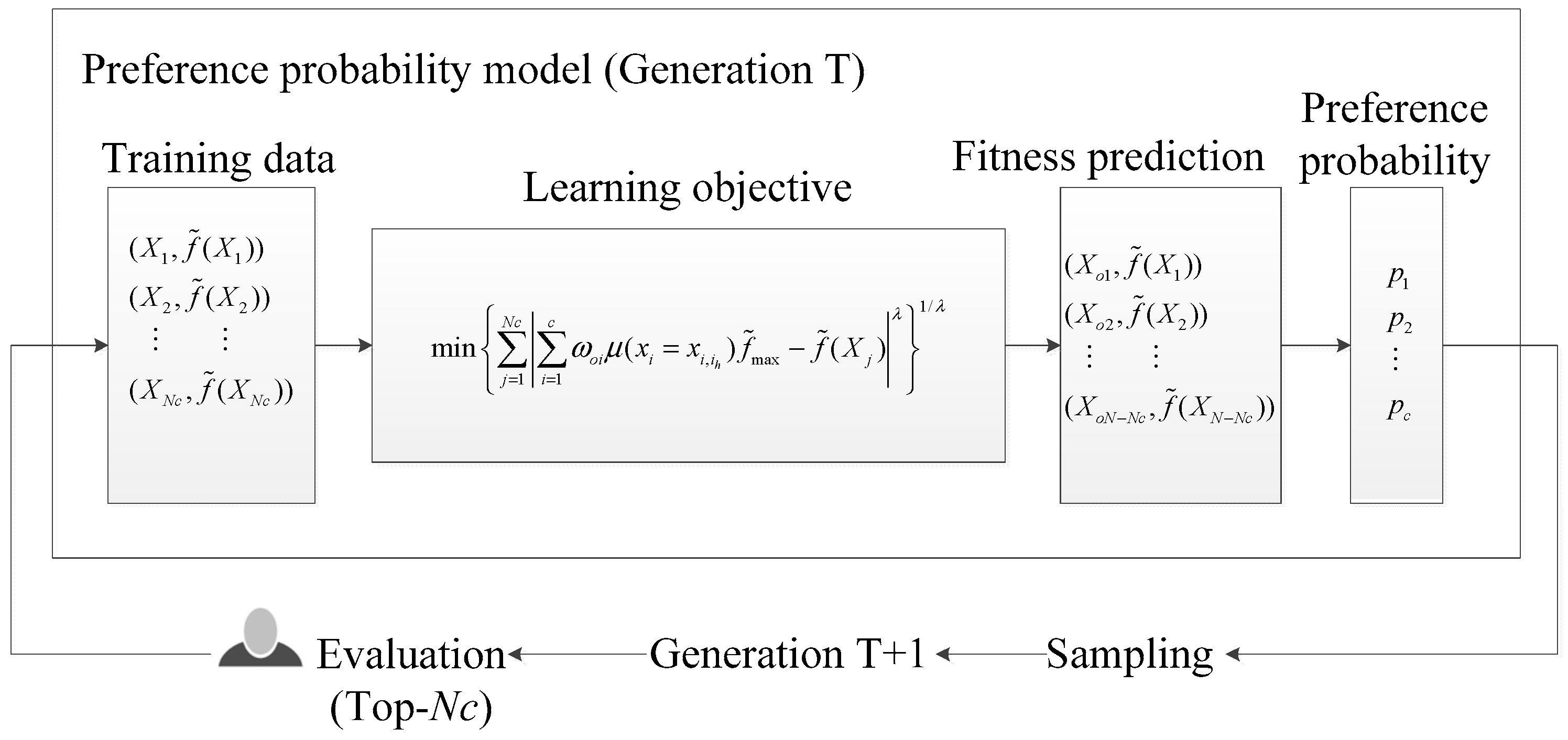
Given this context, this paper proposes a novel preference probability model and surrogate-assisted fitness evaluation method, aiming to achieve an interactive evolutionary solution for OPD within the EDA framework. Firstly, the Top-N algorithm is employed to collect user evaluation information on the Top-Nc individuals. Taking this information as the training samples, a preference probability model based on the similarity of decision variables is then established. Next, individual utility functions are calculated using the similarity of the decision variable, and these utility functions are then used to estimate fitness values for new individuals. Finally, the sampling frequency is updated using the preference probability model, and new individuals are generated through the sampling method in the EDA. Specifically, the main contributions of this paper are as follows:
- (1)
Introducing a probabilistic model to EDA. Unlike machine learning methods, the proposed method is particularly well-suited for small training data and boosts the efficiency of EDA significantly;
- (2)
Presenting a fitness estimation approach that markedly improves the precision of fitness prediction;
- (3)
Proposing a novel interactive distribution estimation algorithm that enhances the quality of the interactive evolutionary algorithm.
3. Experimental Study
3.1. Experimental Setup
To validate the effectiveness of SAF-IEDA, this paper selects the RGB color one-max optimization problem [
22] as a test case. The one-max optimization problem is a specific type of binary function; its objective is to maximize the number of gene positions containing a gene value of 1 within the binary string. The RGB color attributes are from 0 to 255, and its chromosome is encoded as a 24-bit binary string. The first eight bits represent the red attribute (R), the middle eight bits represent the green attribute (G), and the last eight bits represent the blue attribute (B). Each color attribute corresponds to a binary encoding range from 00000000 to 11111111. Clearly, the goal of the RGB color one-max optimization problem is to achieve white color, with attribute values of (255, 255, 255). When solving this problem using interactive evolutionary algorithms, higher user satisfaction implies individuals are closer to the target, making it a typical OPD problem. In this case, there are three decision variables (
c = 3) and 256 attribute values (
m = 256).
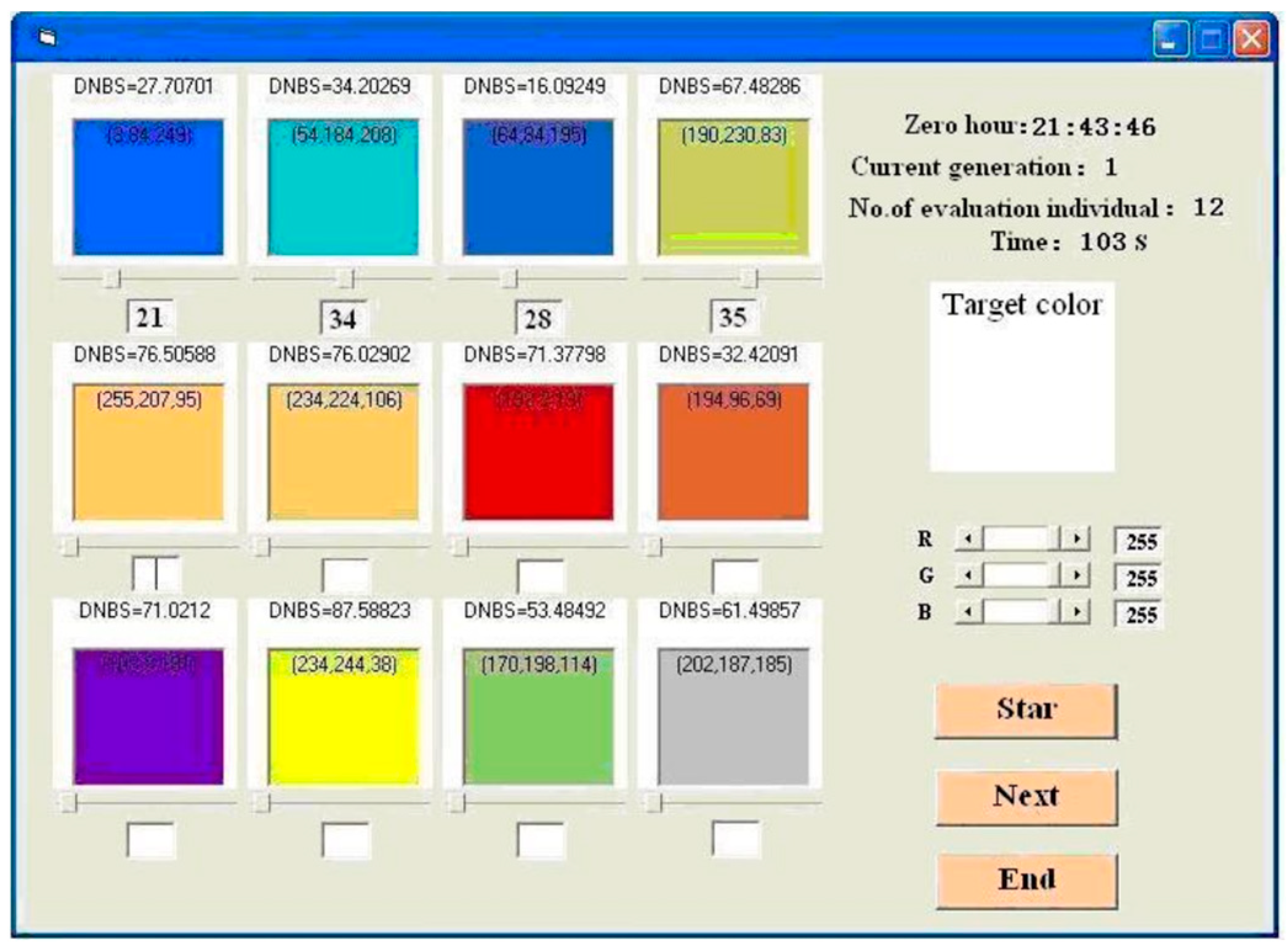
The evolutionary optimization system was developed using Visual Basic 6.0 and executed in the environment with an Intel(R) Xeon(R) E5-2660 V3 CPU at 2.60 GHz and 48 GB RAM. The interactive interface of SAF-IEDA is shown in
Figure 2. The interface presents users with 12 color blocks, i.e.,
Nc = 12. Below each color block, an input textbox for fitness values is provided. Moreover, the system employs slider bars below each color block to record user evaluation time for calculating
. Given that the RGB color space is visually non-uniform, the Munsell color space is introduced to measure the similarity between two colors. The color components are represented by Hue (H), Lightness (L), and Chroma (C). If the National Bureau of Standards unit (NBS) distance of an HLC color pair is less than 3.0, human vision perceives them as similar; if the NBS distance is greater than 6.0, they are regarded as significantly different [
22]. Assuming two HLC color pairs,
and
, their NBS distance (DNBS) is defined as follows:
where
,
,
. The process of converting from the RGB color space to the HLC color space is as follows. Firstly, the transformation from the RGB space to the xyz space is carried out [
22]:
Subsequently, the transformation from the xyz space to the
space is performed:
where
. Further, the transformation is performed to convert the
space to the
space:
where
Finally, the resulting transformation is:
In the experiments, if , we believe two colors are similar. A smaller value indicates a higher similarity between the two color pairs. Thus, this value can also measure the prediction accuracy. A target color block is set on the periphery of each color block, displaying the similarity distance value. The user clicks the “Start” button, and the system generates an initial population randomly. The user evaluates the attributes of the Top-Nc individuals, which forms the initial preference probability vector for EDA. Then, by clicking the “Next” button, the system establishes a preference probability model based on the Top-Nc individuals and their evaluations according to Equation (3) in the background and estimates the fitness values for other unevaluated individuals based on Equation (5). Finally, a new population is generated by sampling according to . For this new population, frequencies of attribute values are calculated, and Pareto dominance sorting is performed based on these frequencies. The Top-Nc individuals are recommended as excellent individuals for further evaluation by the user and will serve as a dominant set used to update the EDA preference probability vector. The cycle continues until the termination condition is satisfied, upon which the “End” button can be clicked to end the evolution. The termination conditions for the algorithm are as follows: (1) , which indicates two colors are within the minimum just-noticeable difference, and the population has produced colors that are very close to the target color or (2) the user has discovered a satisfactory individual, or half of the individuals to be evaluated by users are the same, or the user feels fatigued.
In this study, four representative algorithms are selected as comparison algorithms to validate the effectiveness of SAF-IEDA. These algorithms include:
- (1)
The traditional interactive genetic algorithm (IGA);
- (2)
The Kano-integrated interactive genetic algorithm (Kano-IGA), proposed in [
23];
- (3)
The interactive genetic algorithm with BP neural network-based user cognitive surrogate model (BP-IGA), proposed in [
24];
- (4)
An interactive estimation of the distribution algorithm with RBF neural network-based fitness evaluation (RBF-IEDA), proposed in [
16].
To perform the comparison, five male and five female university students without visual impairments are chosen as test users, labeled as User 1 to User 10. The optimization system is applied, and SAF-IEDA along with the comparison methods is run separately 20 times. The average results are calculated for each run and subjected to comparative analysis.
In all methods, the population size is set to be
N = 200 and the maximum number of generations is set to be
T = 10. For SAF-IEDA, the user’s fitness evaluation range is set as integers from 1 to 99. IGA adopts the k-means clustering strategy, the roulette wheel selection, the single-point crossover with a probability of 0.85, and the mutation with a probability of 0.05. BP-IGA takes a three-layer BP network with a configuration of 12-2-7 as the learning model for surrogate-assisted fitness evaluation and uses the same single-point crossover and mutation as IGA. Kano-IGA utilizes the Kano model to calculate preference values for individual attributes and recommends individuals that align with user satisfaction. This is a relatively new interactive evolutionary algorithm, and its single-point crossover and mutation probabilities are set as 1 and 0.05, respectively. RBF-IEDA constructs a preference surrogate-assisted model by using an RBF network and implements evolutionary optimization based on IEDA, according to the suggestions in reference [
14].
3.2. Results and Analysis
3.2.1. The Parameter
The parameter
in Equation (6) directly impacts the computation of the utility function. Thus, it is essential to investigate the influence of
on SAF-IEDA performance.
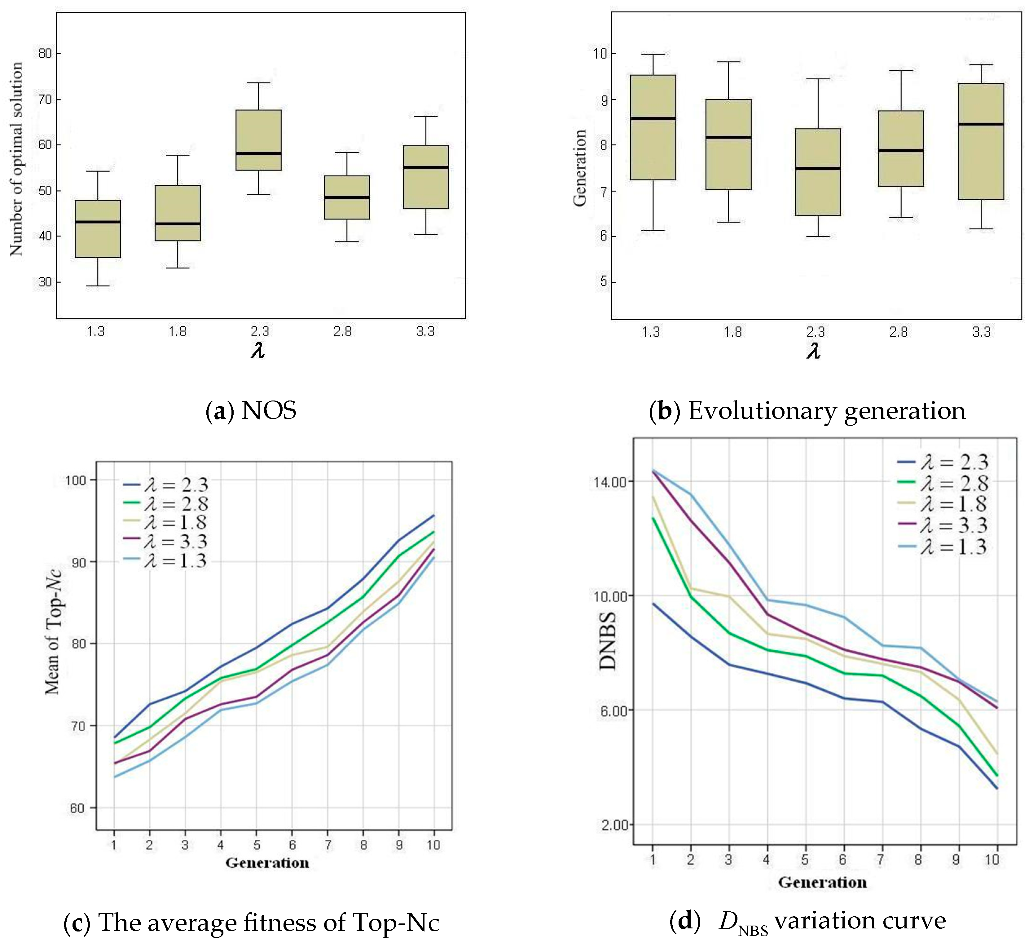
Figure 3a,b show the NOS (the number of optimal solutions) and NG (the number of generations) values obtained using SAF-IEDA under different
(1.3, 1.8, 2.3, 2.8, and 3.3). We can see that both excessively small and large
lead to a decrease in NOS and an increase in the number of generations. The fitness values of the Top-Nc individuals are analyzed statistically, as shown in
Figure 3c. A high value indicates better quality for the recommended individuals. From
Figure 3c, it can be observed that excessively small or large
lead to a decline in the quality of recommended individuals.
Figure 3d illustrates the variations of
under different
. As the evolution progresses,
gradually decreases. Based on the comprehensive experimental results,
= 2.3 is selected as the optimal value.
Table 3 provides the algorithm’s metric values, including means and standard deviations (STD). The success rate (SR) is defined as the number of successful experiments divided by the total number of experiments. As seen in
Table 1, NOS for all users is greater than 160, and the SR is higher than 95%. This indicates that SAF-IEDA effectively solves the RGB color one-max optimization problem.
3.2.2. The Result Analyses of SAF-IEDA with the Comparison Methods
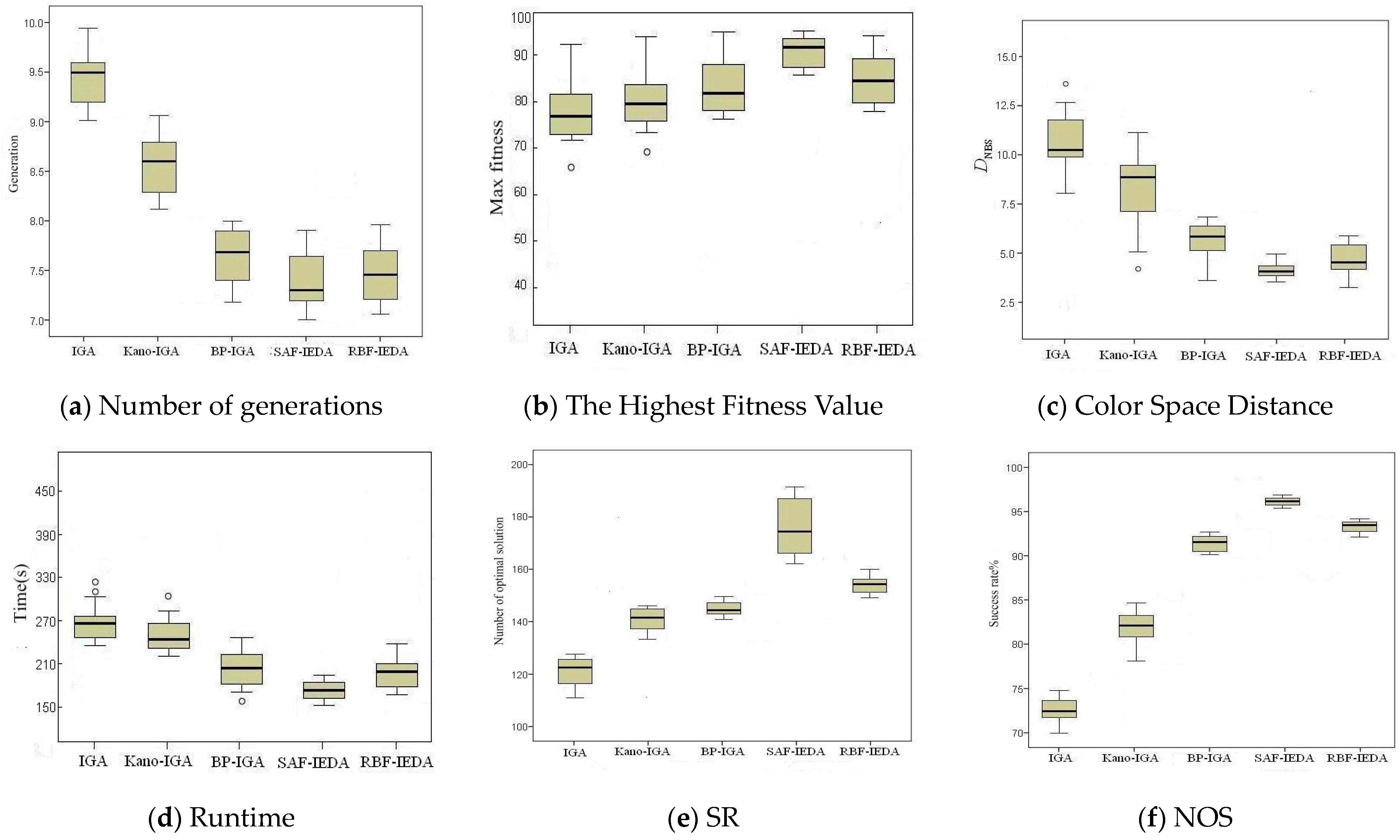
Figure 4 shows the comparison results between SAF-IEDA with the four comparative methods on the six metrics. Here, the circle “o” represents exception values. These six metrics include the number of generations, the highest fitness value, the color space distance, the runtime, NOS, and SR. We can see that SAF-IEDA displays the fewest generations, the highest fitness value, the smallest color space distance, the shortest runtime, as well as the highest NOS and SR values, highlighting the superiority of our method. The reason is that the fitness prediction model based on the preference probability model adopted in this paper is more accurate compared to other methods. Additionally, compared to GA, the EDA-based search engine used in SAF-IEDA has better search performance. In
Figure 4c, it is evident that SAF-IEDA demonstrates the highest fitness prediction accuracy. This can be attributed to the insensitivity of SAF-IEDA to the number of training samples, compared with Kano, BP, RBF, etc. During the initial stages of evolution, the low number of training samples for Kano, BP, and RBF leads to poorer fitness prediction accuracy. In contrast, SAF-IEDA retains good predictive performance with fewer training samples. As the number of iterations increases, the number of training samples also increases; therefore, the predictive accuracy of all methods gradually improves.
Using the Wilcoxon signed-rank test, the results are shown in
Table 4. By observing the positive or negative nature of the
t-values, we can see that SAF-IEDA outperforms the comparison methods in terms of all metrics. On a two-sided significance indicator, although SAF-IEDA does not exhibit significant differences from BP-IGA and RBF-IEDA in terms of the number of generations, there are significant differences between SAF-IEDA and the comparative methods.
SAF-IEDA can achieve high-quality solutions with the lowest errors under the same number of iterations, compared with BP-IGA and RBF-IEDA. This further validates the superiority of SAF-IEDA. Although Kano-IGA also updates the population based on individual attribute preference values dynamically, its metric values are less than SAF-IEDA, suggesting that SAF-IEDA is more accurate in characterizing attribute preferences, and the quality of recommended individuals is higher.
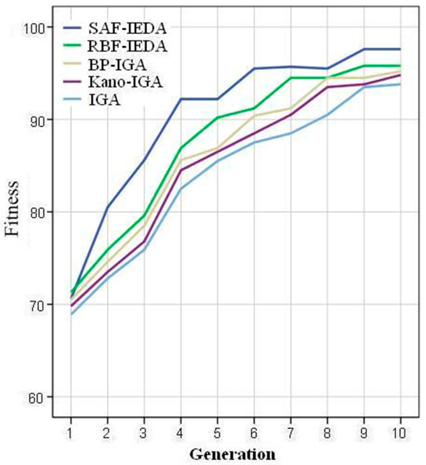
Figure 5 illustrates the convergence curves of the five methods. It is evident that all methods are able to converge, but SAF-IEDA achieves the highest fitness values and shows better convergence.
3.2.3. Application to the Indoor Lighting Optimization
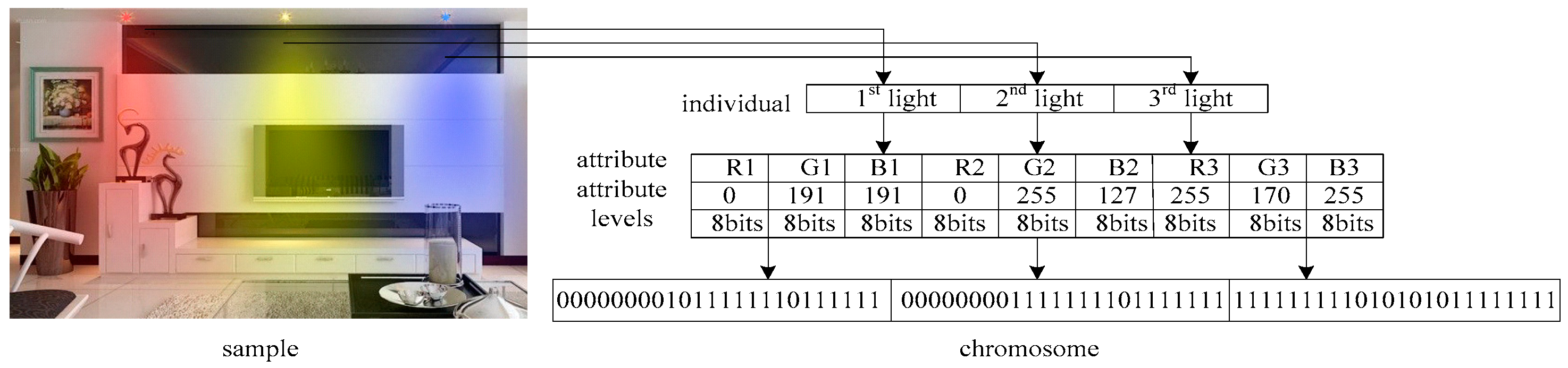
To further validate the effectiveness of SAF-IEDA, SAF-IEDA is applied to optimize the indoor lighting problem. In this scenario, an individual represents a combination of three LED color lights, each comprising three color channels: red (R), green (G), and blue (B). The optimization objective is to create the most favorable light and shadow effects by combining these three-color lights. The RGB variables collectively form a chromosome with a total of nine color attributes. Each RGB variable can take on values in the range of 0 to 255, and these attribute values are encoded using 8-bit binary code. Consequently, a chromosome comprises 72 bits of binary code. Refer to
Figure 6 for a visual representation of the chromosome encoding process. It is important to note that the indoor lighting optimization problem involves a multitude of individual attributes and attribute values, rendering it a complex problem suited for resolution using our method.
Ten users are tasked with optimizing indoor lighting schemes to achieve a ‘warm’ style. These users are not constrained by a maximum number of evolution generations. Comparative methods are run independently ten times, and the results of independent sample analyses for different evolution indicators are presented in
Table 5. The Levene’s test results for each indicator indicate that there are no significant differences in variances among the samples, as all
p-values were greater than 0.05. However, there is a notable significant difference in the number of evolution generations required and the running time between SAF-IEDA and the comparative methods. This suggests that when there is no restriction on the maximum number of evolution generations, Kano-IGA, BP-IGA, and RBF-IEDA require more evolution generations and more time to achieve high-quality satisfactory solutions, likely due to the high training costs associated with their models. IGA performs the worst and requires more evolution generations to obtain satisfactory solutions. There is a significant difference in terms of the highest fitness value, color space distance, and optimal solution quantity between SAF-IEDA and the comparative methods, indicating that it is suitable for personalized optimization objectives. Therefore, SAF-IEDA can achieve higher-quality solutions and better interactivity.
Based on the above analysis, it is evident that SAF-IEDA outperforms the comparative methods for various optimization objectives. In all comparison indicators, SAF-IEDA consistently delivers the most satisfactory optimization solutions. Therefore, it can be concluded that SAF-IEDA is superior to comparative methods in addressing the indoor lighting optimization problem effectively.
4. Conclusions
This paper proposed a preference probability model and a surrogate-assisted fitness evaluation strategy under the framework of an interactive distribution estimation algorithm. In traditional EDA, individual fitness is an explicit function value, and new individuals are generated using sampling based on the probability model of individual attributes. In an interactive evolutionary environment, individual fitness needs to be set by the user, and it reflects the user’s preferences. In this case, the distribution of individual attributes is consistent with the preference distribution. User preferences depend on the similarity of individual phenotypes, which can be described by Gaussian functions for decision variables. In this way, a preference probability model can be established based on the similarity of decision variables, and generating new individuals using this preference probability model will better align with user preferences. On the other hand, in order to alleviate fatigue, utility functions are used to express attribute preferences and weighted estimates of fitness values to better reflect consistency between attributes and preference distributions. The strategy proposed in this article is an extension of EDA applied in an interactive evolutionary environment. This method is based on distribution estimation algorithms, uses a preference probability model as sampling probabilities, and utilizes Top-Nc individuals to construct a preference probability vector for evaluating fitness values based on the utility function.
The experimental results on the RGB color one-max optimization problem and the indoor lighting optimization problem show that users can obtain the most satisfactory optimization solution using SAF-IEDA, compared with five existing comparison algorithms. This paper only deals with single-objective optimal problems; in-depth research is needed for cases with multiple objectives. In addition, applying the proposed method to more practical optimal product design problems is also an open issue.


