Article

Integrated Optimization of Blocking Flowshop Scheduling and Preventive Maintenance Using a Q-Learning-Based Aquila Optimizer

College of Information Science and Engineering, Northeastern University, Shenyang 110819, China
*
Author to whom correspondence should be addressed.
Symmetry 2023, 15(8), 1600; https://doi.org/10.3390/sym15081600
Submission received: 17 July 2023 / Revised: 12 August 2023 / Accepted: 16 August 2023 / Published: 18 August 2023
(This article belongs to the Special Issue Symmetry in Optimization and Its Applications to Machine Learning)

Abstract

:
In recent years, integration of production scheduling and machine maintenance has gained increasing attention in order to improve the stability and efficiency of flowshop manufacturing systems. This paper proposes a Q-learning-based aquila optimizer (QL-AO) for solving the integrated optimization problem of blocking flowshop scheduling and preventive maintenance since blocking in the jobs processing requires to be considered in the practice manufacturing environments. In the proposed algorithmic framework, a Q-learning algorithm is designed to adaptively adjust the selection probabilities of four key population update strategies in the classic aquila optimizer. In addition, five local search methods are employed to refine the quality of the individuals according to their fitness level. A series of numerical experiments are carried out according to two groups of flowshop scheduling benchmark. Experimental results show that QL-AO significantly outperforms six peer algorithms and two state-of-the-art hybrid algorithms based on Q-Learning on the investigated integrated scheduling problem. Additionally, the proposed Q-learning and local search strategies are effective in improving its performance.

1. Introduction

In the field of intelligent manufacturing, manufacturers are generally aiming at more reliable production systems. However, both deterioration and default of machines are becoming critical factors because they inevitably appear in practical production systems [1,2]. In such a scenario, machines are not idealized, and they can break down and deteriorate with cumulative processing time. To restore machine efficiency and reduce faults, executing preventive maintenance (PM) is necessary [3]. Nevertheless, making decisions solely from one side of production or PM is seriously hard to reach a good scheduling solution since they are in conflict with each other. Specifically, PM consumes production time, whereas delaying PM to ensure production on time may increase the probability of machine faults. To this end, integrated optimization of production and PM has become an effective method to handle such problems [4]. In the integrated optimization process, degradation and default of machines are considered, and PM is regarded as a constraint to simultaneously optimize production and PM. In recent years, a large number of studies have demonstrated that this integrated optimization method can achieve a high-quality solution [5]. Consequently, this study aims to optimize an integrated production and PM problem.
Flowshop is a well-known manufacturing system for production scheduling, and complex manufacturing plants often can be abstracted into variants or combinations of this system [6]. Blocking flowshop is one of the most important variants of flowshop. It has limited buffer capacity between machines due to the process characteristics and technological requirements, and it has significant practical applications, e.g., chemical production [7], steel industry [8], and robotic scheduling [9]. The reason of the blocking may be that jobs are stranded in machines due to the lack of workers, or certain stages are not allowed to be stored [10]. Due to the important practical significance, this study investigates the integrated optimization of blocking flowshop. A general situation, i.e., the blocking flowshop with no intermediate buffers is taken as the research object. In this situation, a job cannot leave a machine until the next machine is free. Following the three-field notation proposed by Graham et al. [11], the problem studied in this paper can be expressed as F m P M , b l o c k i n g ω 1 C m a x + ω 2 T M C , where F m means the flowshop, P M represents the preventive maintenance, b l o c k i n g indicates the blocking scheduling, and ω 1 C m a x + ω 2 T M C denotes the object with minimizing the weighted sum of completion time and total maintenance cost.
In terms of algorithm, since the classical blocking flowshop with three or more machines has been proven to be NP-hard [12], it is even more NP-hard for a blocking flow shop with an integrated optimization. It is difficult to obtain a satisfactory solution in a short time for large-scale problems with exact and heuristic algorithms. Therefore, various swarm intelligence algorithms are often as fast and effective tools of solving such problems [13], such as genetic algorithms (GA) [14], particle swarm optimization algorithms (PSO) [15], and bee colony algorithms (ABC) [16]. However, for complex integrated optimization problems, especially large-scale problems, swarm intelligence algorithms often easily fall into local optimal solutions. Thus, scholars are continuously designing high-performance search mechanisms to handle such problems. The aquila optimizer (AO) is a recently developed swarm evolutionary algorithm that simulates the hunting behavior of aquila using multiple update strategies. Recent studies [17] have revealed that AO has advantages of strong search capabilities and fast convergence. Moreover, it has been well applied to problems such as path planning [18], 0–1 backpacking [19] and network node localization [20]. Therefore, in this work, the high-performance AO is used to get a better solution.
The presence of PM and blocking increases the complexity of the scheduling, making it a complex, coupled, and symmetric combinatorial optimization problem. In order to cope with the considered problem with high performance, it is necessary to adopt some strategies to enhance the search capability. In recent years, Q-learning (QL) has become a valid tool to improve intelligent algorithms in the field of scheduling, and the improved algorithms always obtain an excellent performance. For instance, Runfo Li et al. [21] used QL to dynamically adjust the crossover and variance probabilities of GA for the port ship scheduling problem. Mao et al. [22] used QL to select the update strategies of brain storm optimization algorithm for the assembly flow shop scheduling problem. Lixin Cheng et al. [23] designed a QL based on the population size adjustment mechanism for the energy-efficient manufacturing scheduling problem. Zhang et al. [24] designed a QL based ant colony algorithm for an assembly scheduling, where QL is adopted to adjust the search parameters. Learning from the previous studies, this study proposes a QL-based AO (QL-AO), wherein QL is applied to adjust the selection probabilities of the four update strategies of the basic AO. Additionally, a set of local search strategies is designed according to the problem features. To verify the performance of QL-AO, computational experiments are performed. The results show that the proposed algorithm can gain better results when solving the proposed problem.
The contributions of this work are as follows:
(1)
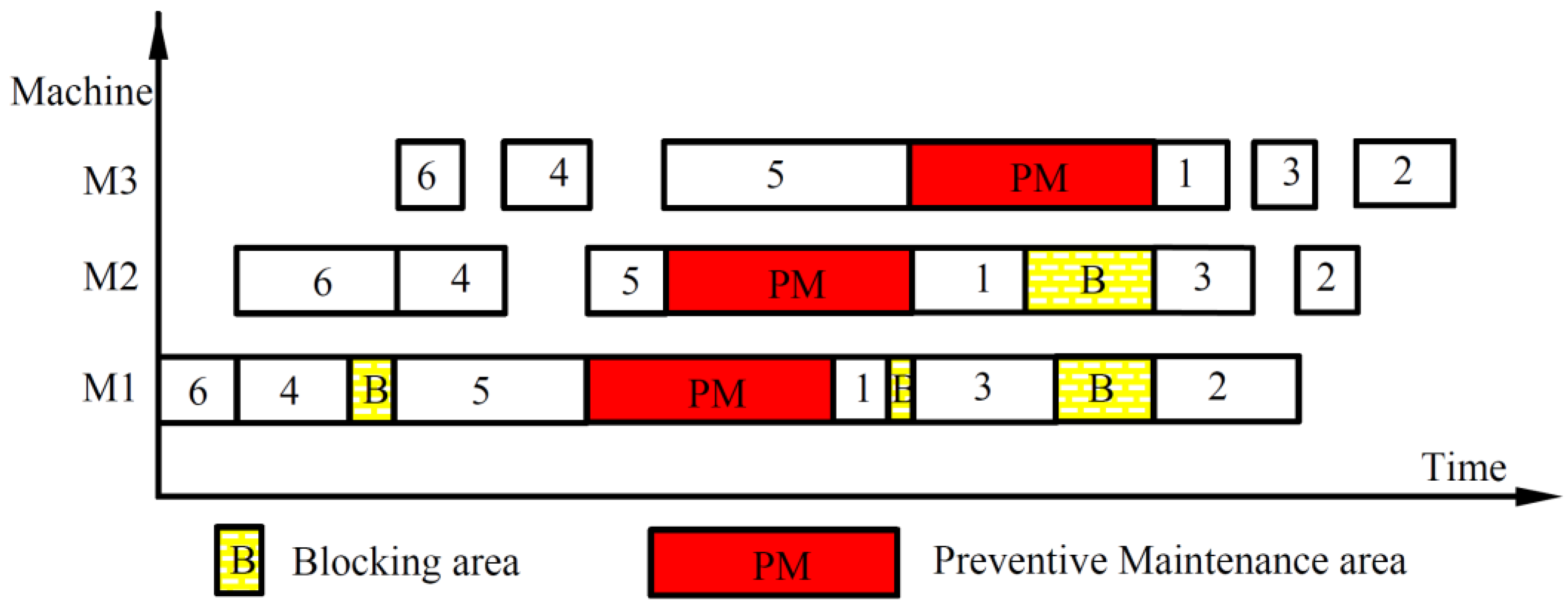
This work formulates an integrated optimization model for a blocking flowshop scheduling problem. In this model, deterioration and default of machines, as well as machine maintenance are considered at the same time. To calculate the object values, a recursive formula is established;
(2)
This work develops an AO with some special search techniques to enhance its performance and propose the improved algorithm QL-AO. It employs a QL-based mechanism for strategies selection. Other than that, a set of local search strategies is designed to strengthen the search ability via combining the problem’s features;
(3)
This work conducts a series of experiments to evaluate the performance of the proposed QL-AO by comparing it with eight peer algorithms. They are experiments of parameter settings, components comparison and algorithm comparison. The achieved results suggest that QL-AO is an efficient optimizer compared to its peers.
The remainder of this paper is outlined as follows: Section 2 describes the problem scenario and builds a mathematical model. Section 3 presents the designed algorithm. Section 4 implements numerical experiments and analyzes the results. Section 5 concludes this paper and provides some future research directions.

2. Problem Description

This study investigates an integrated optimization problem of blocking flowshop scheduling and preventive maintenance (PM), in which both deterioration and default of machines are also considered. The problem description is laid out in the following sections.
There are n jobs arriving at the initial time to be processed once on m machines in turn. The sequence of processing jobs on all machines is the same as the first machine. Due to the presence of blocking, the processed job must wait for the next operation on the current machine until the next machine is available for processing. It is noted that two special factors, that is, deterioration and default of machines, are both taken into account on the basis of classic blocking flowshop scheduling. This means that the actual processing time of job requires to be determined by the deterioration and failure parameters of the machine. The purpose of integrated scheduling is to find the optimal job processing sequence J k , ( k = 1 , 2 , , n ) , as well as to determine when to execute PM activity.
For machine deterioration, let p i , j denote the normal processing time of i -th job on machine j , a i , j denote the machine age of machine j after processing the i -th job, and γ i denote the deterioration factor of machine j . The processing time of i -th job on machine j can be calculated as p i , j = p i , j + γ i a i , j 1 when considering linear deterioration [25].
For machine fault, the Weibull distribution is adopted here according to the work of Wang et al. [26]. The expected number of failures when machine j processes the i -th job i can be calculated as N i j   = a i , j 1 a i , j r t d t =   a i , j η β a i , j 1 η β , where β is the shape parameter and η is the scale parameter. Once fault occurs, corrective maintenance (CM) is executed immediately. CM can only restore the operating state of the machine but not restore the machine age. In this study, the execution time of CM is included in the actual processing time. Therefore, the actual processing time after considering the machine faults and CM can be calculated as p i , j =   p i , j + N i j t c m , where t c m is the time for executing a CM.
This study employs a threshold-based PM strategy to ensure that the machine operates at a consistently high level of reliability [27]. Specifically, the machine undergoes PM every TPM (Time Period of Maintenance) to avoid potential fault or performance degradation. The TPM should always be less than the maximum age limit T m a x j . Here, T m a x j can be calculated as T m a x j = η · e x p ( ln ( ln R j ) β ) , where R j is the minimal reliability threshold of machine.
Based on this policy, the execution of PM can be determined after obtaining the scheduling sequence. To resolve any potential conflict between PM and job processing, this study employed a conservative PM insertion approach. When scheduling a job, the first step is to calculate whether the machine age exceeds T m a x j after processing. If the limit is exceeded, the processing of this job is immediately delayed, and the PM is inserted at the end of the previous job. If the threshold is not exceeded, normal processing the job without executing PM. Therefore, the PM decision matrix can be defined as p m i , j 1 = 0 , i f   a i , j T m a x j 1 ,   e l s e , where p m i , j 1 = 1 denotes executing PM and restoring the machine age, i.e., set a i , j 1 = 0 , and p m i , j 1 = 0 denotes no execution of PM and calculating the machine age a i , j = a i , j 1 + p i , j .
To further explain the impact of PM and blocking on scheduling, let us consider a 3 × 6 scheduling example, as depicted in Figure 1. Regarding PM, when machine 1 is processing job 5, an immediate execution of job 1 would exceed the machine’s maximum age limit. Therefore, PM is inserted after job 5’s processing, leading to the postponement of job 1’s processing. Regarding blocking, during the processing of job 4 on the first machine, job 6 is concurrently being processed on machine 2. Since there is no intermediate buffer, job 4 remains on the first machine until job 6 completes its processing. Consequently, job 4’s transportation to machine 2 for processing is delayed, thereby causing a subsequent delay in starting job 5.
The recursive formula to calculate the makespan ( C m a x ) is proposed as shown in Equations (1)–(6). This formula is an extension of the standard blocking flowshop recursive formula [28]. In the recursive process, the calculation starts with determining the completion time of the first job. Then, the departure time is calculated, followed by determining the completion time and departure time of the second job. This process continues iteratively until reaching the last job. And then, C m a x is obtained.
C 1 , j = l = 1 j p 1 , l , j = 1 , , m .
D 1 , j = C 1 , j , j = 1 , , m .
D i , 0 = D i 1,1 , i = 2 , , n .
C i , j = max [ C i 1 , j + T p m j × p m i 1 , j , D i , j 1 ] + p i , j , i = 2 , , n , j = 1 , , m .
D i , j = m a x C i , j , D i 1 , j + 1 , i = 2 , , n , j = 1 , , m 1 .
C m a x = C i , m = D i , m , i = 2 , , n .
Notably, D 1 , j represents the start time of the first job on machine j. Due to the presence of PM, the other job’s start time on the machine j depends on the completed time for PM and the departure time of the last job. The computation of p i , j and p m i , j has been detailed in the preceding paragraphs.
The objective function in this study considers not only the widely used metric C m a x , but also the substantial costs associated with maintenance activities. The goal of the problem is to minimize the weighted sum of the C m a x and the total maintenance cost, which encompasses both PM cost and CM cost. The total maintenance cost is calculated by multiplying the total number of maintenance activities by the unit price of each. The mathematical representation of the objective function is provided in Equation (7).
Min   o b j = ω 1 C m a x + ω 2 [ C P M × i = 1 n j = 1 m N i , j + C M R × i = 1 n j = 1 m p m i , j ]
where ω 1 , ω 2 are weighting factors, and CPM, CMR are the cost of performing once PM and CM, respectively.

3. The Proposed Algorithm

3.1. Basic Aquila Optimizer

Aquila optimizer (AO) is a novel population-based swarm intelligence algorithm proposed by Laith Abualigah et al. [29] in 2021, which simulates the hunting process of aquila. In the framework of AO algorithm, there are four key population update strategies termed as expanded exploration, narrowed exploration, expanded exploitation and narrowed exploitation. The whole iteration process of AO can be divided into two periods. In the first 2/3 iterations, that is regarded as the exploration period, expanded exploration and narrowed exploration strategies are selected randomly to update the population. In the last 1/3 iterations, that is regarded as the exploitation period, expanded exploitation and narrowed exploitation strategies are employed randomly, as shown in Algorithm 1.
Algorithm 1: Basic AO
1.
Initialize the population X and the parameters (i.e., α, δ, etc.) of the AO;
2.
Calculate the fitness values of individuals in the population and find X b e s t t ;
3.
Set t = 0;
4.
While (the end condition is not met) do
5.
for each individual in the current population do
6.
    Update X m e a n t , x , y , Q F t , L e v y D ;
7.
    if t 2 3 i t e r m a x
8.
        if rand ≤ 0.5
9.
        Update the current individual using expanded exploration;
10.
      else
11.
         Update the current individual using narrowed exploration;
12.
      end if
13.
     else
14.
        if rand ≤ 0.5
15.
         Update the current individual using expanded exploitation;
16.
        else
17.
         Update the current individual using narrowed exploitation;
18.
        end if
19.
     end if
20.
   end for
21.
   Update X b e s t t ;
22.
   T = t + 1;
23.
end while
24.
return The best solution ( X b e s t ).
For expanded exploration strategy, the AO widely explores high soar to determine the area of the search space, as shown in the following formula.
X t + 1 = X b e s t t × 1 t i t e r m a x + X m e a n t X b e s t t × r a n d
where t is the current iteration, i t e r m a x is the maximum iteration, X b e s t t is the best individual in the t-th iteration, and r a n d is the uniformly distributed random numbers between 0 and 1. X m e a n t denotes the locations mean value of the current population connected at t-th iteration, defined as X m e a n t = 1 N i = 1 N X i t .
For narrowed exploration strategy, AO narrowly explores the selected area of the target prey in preparation for the attack, as shown in the following formula.
X t + 1 = X b e s t t × l e v y D + X r a n d t + y x × r a n d
where X r a n d t is an individual selected randomly from the population in the t-th iteration. y and x are used to present the spiral shape in the search, which are calculated as x = r × s i n ( ϕ ) , and y = r × cos ϕ . r = r 1 + 0.00565 × D 1 , and ϕ = 0.005 × D 1 + 3 π 2 , where r 1 is a parameter between 1 and 20 for fixed the number of search cycles, and D 1 is integer numbers from 1 to the length of the search space.
L e v y D is the Levy flight distribution function used to enhance the randomness of the search, as shown in Equation (10).
L e v y D = s × u × σ v 1 / λ , σ = Γ 1 + λ × s i n e π λ 2 Γ 1 + λ 2 × β × 2 λ 1 2
where D is the dimension of the individual and Γ · is the gamma function. The constant parameters s and λ are set to 0.01 and 1.5, respectively, and the random parameters u and v are taken between 0 and 1.
For expanded exploitation strategy, AO exploits the selected area of the target to get close to the prey and attack, as shown in the following formula.
X t + 1 = ν × X b e s t t X m e a n t r a n d + δ × U B L B × r a n d + L B
where U B and L B are the upper and lower bounds, respectively. ν and δ are both the exploitation adjustment parameters.
For narrowed exploitation, AO attacks the prey over the land according to their stochastic movements, as shown in the following formula.
X t + 1 = Q F t × X b e s t t G 1 × X t × r a n d G 2 × L e v y D + G 1 × r a n d
where Q F t is a quality function defined as Q F t = 2 × r a n d 1 t 1 i t e r m a x 2 , which is used to balance the search strategy. G 1 = 2 × r a n d 1 is used to simulate the action of tracking prey, and G 2 = 2 × 1 t i t e r m a x is used to represent the slope of the flight.

3.2. Individual Representation

Considering that the AO algorithm requires to utilize the individuals with continuous encoding to search for the optimal processing sequence of jobs of the investigated scheduling problem, a random key representation-based ROV rule [30] is used to accomplish the mapping of individual and candidate solution in this study. For example, let us consider an individual X = [ 0.82 , 0.18 , 0.23 , 0.68 ] , where the minimum value 0.18 is at position 2. This indicates that job 2 will be the first to be processed. Next, the sub-minor value 0.23 is at position 3, indicating that job 3 will be the second to be processed. So, the corresponding candidate solution, that is, the processing sequence of 4 jobs, is J = 2 , 3 , 4 , 1 .
In order to enhance the quality of the initial population, an NEH heuristic is used to generate a number of initial individuals with higher fitness. In detail, a candidate solution of flowshop scheduling is firstly achieved according to the NEH heuristic, and then 10% individuals in the initial population are generated randomly by executing the abovementioned ROV rule upon the achieved solution reversely.

3.3. Q-Learning-Based Strategies Selection

The balance of exploration and exploitation is very important to intelligent algorithms [31]. In the basic AO, the selection probabilities of four population update strategies are artificially fixed. To cope with the complex integration scheduling problem, a Q-learning (QL)-based selection method is proposed, which is the major contribution of this study. In the proposed selection method, QL is employed to dynamically adjust the selection probabilities of population update strategies according to the feedback information of AO’s iteration process. The procedure of the QL update process is given in Algorithm 2. The state, action and reward are presented below.
State: There are 12 states in the state set. It is divide into two metrics, that is c b a d and p o p d i v , as shown in Table 1. Here, c b a d is the cumulative unimproved frequency of historical optimal solutions, and c 1 , c 2 , d 1 , d 2 , d 3 are the division parameters. The p o p d i v represents the population diversity as shown in Equations (13) and (14) [32].
p o p d i v = k = 1 D η D f q k ( 1 f ( q ) k ) D 1
where f ( q ) k is defined as Equation (14). For notation δ i , j q , if the j -th job processed by the machine i is job q , then δ i , j q is set to 1, otherwise it is set to 0.
f ( q ) k = i = 1 p o p n u m j = 1 D δ i , j q p o p n u m , q , k = 1 , , D
Action: Action set A is composed of four actions. They are defined as increasing the selection probabilities of four update strategies. For example, let Δ ξ denote the amount of probability increase, and p 1 denote the selection probability of expanded exploration. Action 1 can be described as p 1 p 1 + Δ ξ . To ensure that the probability sum is 1 after the action is executed, the selection probabilities are normalized as p i = p i / i = 1 4 p i . The well-known ε-greedy strategy is used to select an action, as described in lines 10–14 in Algorithm 2. In addition, to expedite the convergence of QL, the ε value undergoes a linear decrease from 0.9 to 0.01 within every 100 iterations.
Reward: The reward method is described in lines 2–8 in Algorithm 2. If the optimal solution is improved, the reward is set to 20. If the optimal solution does not improve but there is an increase in diversity, the reward is set to 10. If neither of these conditions is met, the reward is set to −5.
Algorithm 2: Pseudo code of Q-learning update
Input: A , Q, s, c b a d , p o p d i v ,   c 1 , d 1 , f b e s t t , f b e s t , ε .
Output: Q, a′, s′.
1.
  Get the new state s by   c b a d , p o p d i v ,   c 1 , d 1 based on the rules in Table 1.
2.
  If  f b e s t t < f b e s t
3.
   r = 20
4.
  else if  p o p d i v > 0
5.
   r = 10
6.
  else
7.
   r = 5
8.
  end if
9.
   Q s , a 1 α Q s , a + α r + γ · m a x a A Q s , a
10.
if rand > ε
11.
a a r g m a x a A Q s , a
12.
else
13.
a r a n d o m C h o i s e ( A )
14.
end if

3.4. Local Search Strategies

In order to further enhance the search performance, five search strategies are used, which can be described as follows.
  • Machine Age-Based Insert (MI): Insert the job with the highest mean machine age (the average value of machine age for all machines) after the job with the lowest mean machine age but excluding the first job. By applying this strategy, the job with the highest mean machine age is repositioned to a more favorable location. This approach may find a more potential solution.
  • PM-Based Swap (PS): In this strategy, the job with the maximum total times of PM is moved one position backward. By performing this swap operation, the algorithm aims to explore different arrangements of the PM-intensive job, potentially leading to improvements in the scheduling solution.
  • Job Insert (JI): This is a common local search strategy in that two different jobs are randomly selected and the first job is inserted after the second job. This operation introduces a change in the sequence of jobs and may lead to an improved solution.
  • Job Swap (JS): Another commonly used local search strategy is job swap. Two different jobs are randomly selected, and their positions are swapped. This exchange alters the job order, potentially resulting in a better scheduling solution.
  • Random Generation (RG): This strategy randomly generates a scheduling solution. The purpose of this strategy is to introduce diversity into the population. It encourages the discovery of novel and potentially better scheduling solution.
For executing the five local search strategies, the population is first sorted according to objective values. The top 20% individuals use MI and PS with equal probability. The bottom 20% use RG, and the other individuals use JI and JS with equal probability. Among all the local search strategies, the new solution is accepted if it improved, otherwise not.

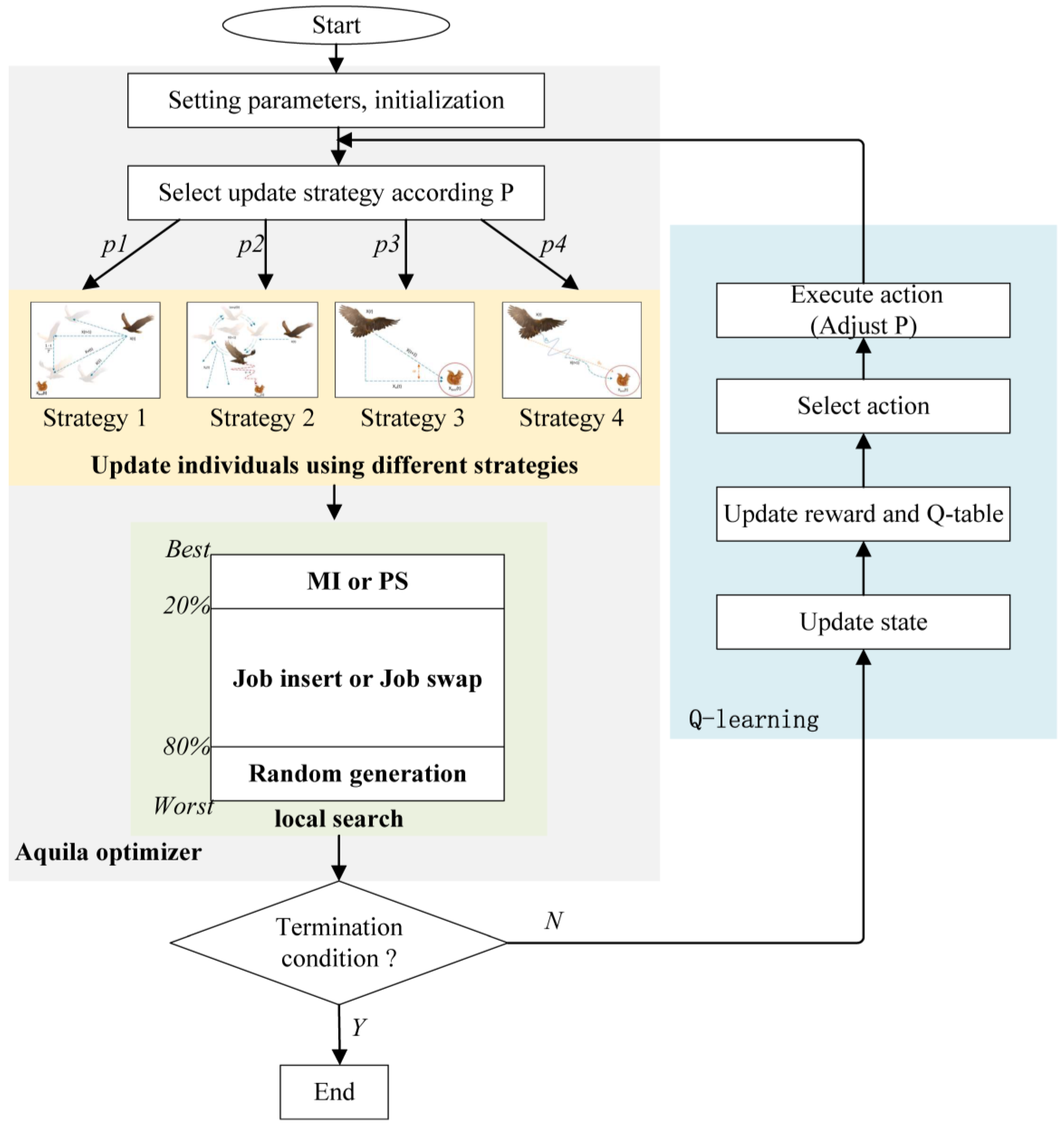
3.5. The Framework of Proposed Algorithm

The proposed algorithm termed as QL-AO is an effective combination of AO and QL to further improve the performance of AO for the investigated problem. The detailed steps of QL-AO are presented below and the flow chart is shown in Figure 2.
(1)
Initialize the population with 90% random individuals and 10% ones generated via the NEH-based solution.
(2)
Select update strategy for each individual according to selection probabilities and then update the population using different strategies.
(3)
Execute local search for each individual to further improve its quality.
(4)
If the termination condition is not met, execute a new iteration after adjusting the selection probabilities by QL; otherwise, the algorithm is terminated.
(5)
Go to QL section. Update the system state, reward, and Q-table. Select the new action, execute the action to adjust probabilities, and then go to step (2).

4. Computational Experiments

In this section, a series of experiments are conducted to evaluate the performance of the proposed QL-AO algorithm for the investigated integrated optimization problem of blocking flowshop scheduling and preventive maintenance. All algorithms run on a computer with an Intel Core i5-10500 @ 3.10 GHz CPU and 16 GB memory and all the algorithms are coded in the software platform MATLAB 2017a.

4.1. Test Instance Settings

In total, the 19 test instances are generated according to two flowshop scheduling benchmark, in which the first 12 are proposed by Taillard [33] and the last 7 come from the work of Ruiz [34], respectively. Additionally, we set the parameters of machine failure and maintenance as follows: two parameters of Weibull distribution β = 2 and η = 7000 , deterioration factor γ = 0.02 , two parameters of maintenance time t c m = 20 and t p m = 100 , and reliability threshold R = 0.85 .

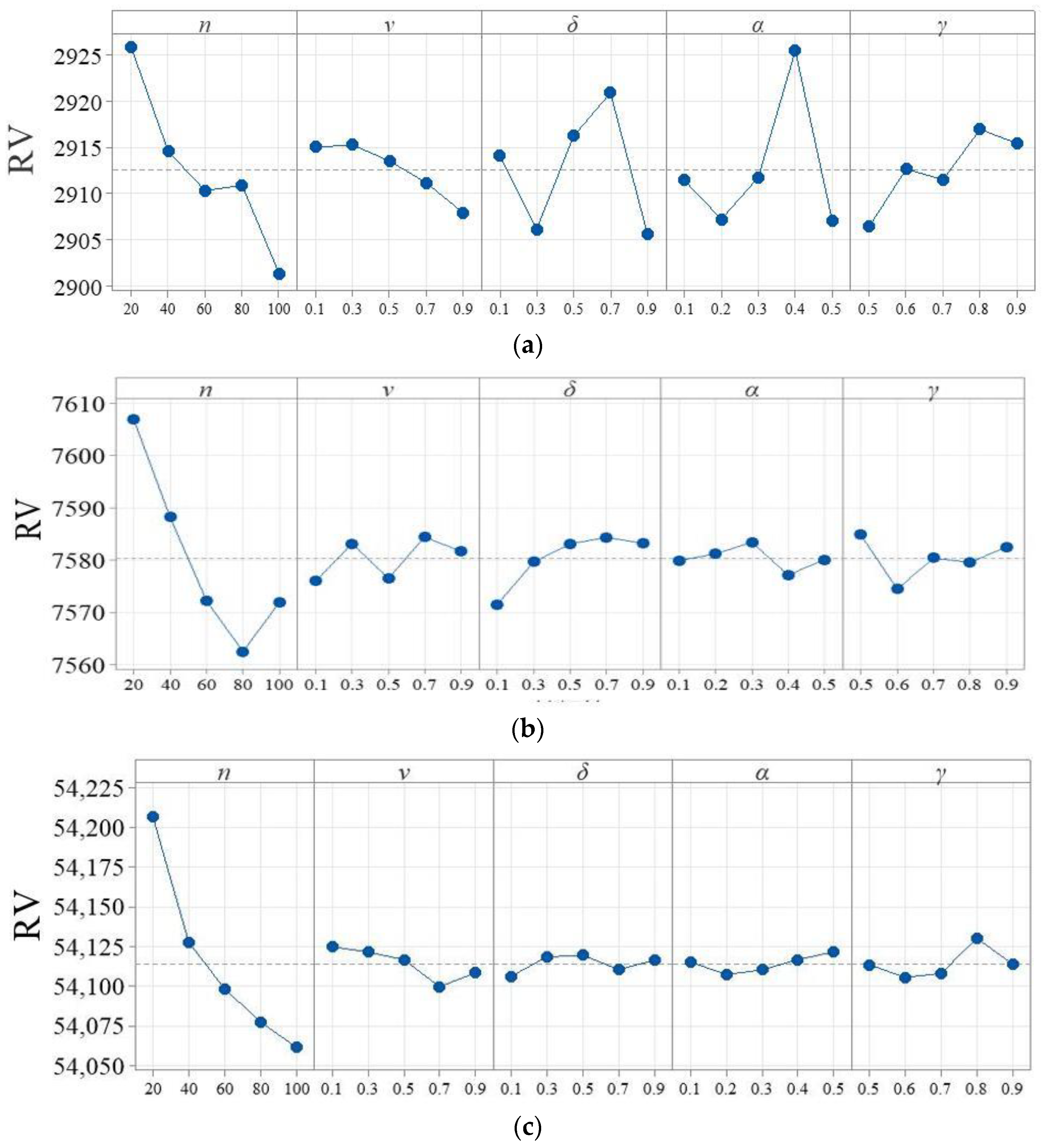
4.2. Key Parameter Settings

In the proposed QL-AO algorithm, there are five key parameters, i.e., the population size n , two exploitation adjustment parameters ν and δ , two QL-related parameters α and γ . To find the promising parameters for the algorithms and the sensitivity analysis of parameters, the Taguchi’s orthogonal experiment approach was employed. In this part, three sets of orthogonal experiments were conducted, respectively, on a small-scale instance (with 20 jobs and 20 machines), a medium-scale instance (with 100 jobs and 5 machines), and a large-scale instance (with 400 jobs and 20 machines). In each group of experiment, 5 parameter levels were chosen for each parameter and an orthogonal array with 25 parameter combinations was picked. QL-AO with each parameter combination was run 20 times, and the mean value of the object over 20 independent runs was determined as the response variable (RV), as shown in Table 2. Additionally, Table 3 shows the significant rank of parameter combinations, and the results of the orthogonal experiments are shown in Figure 3.
It can be observed from the main effects plots that n = 100 , ν = 0.9 , δ = 0.9 , α = 0.5 , γ = 0.5 is a promising parameter combination for small-scale instances; n = 80 , ν = 0.1 , δ = 0.1 , α = 0.4 , γ = 0.6 is a promising parameter combination for medium-scale instances; n = 100 , ν = 0.7 , δ = 0.1 , α = 0.2 , γ = 0.6 is a promising parameter combination for large-scale instances. From Table 3, it is observed that population size n is the most significant parameter for all situations. An appropriate increase in n is beneficial to the search. The ranking of two exploitation adjustment parameters ν , δ increases and decreases, respectively, with the increase in scale of the instances. This suggests that in large-scale instances, the parameter ν is more important. The learning rate α is ranked low in the medium-scale and large-scale instances but is ranked high in the small-scale instance. This suggests that only the small-scale instances are more sensitive to the setting of the learning rate. The importance of the discount rate γ is not much affected by the scale of the instances, and it keeps around rank 3.

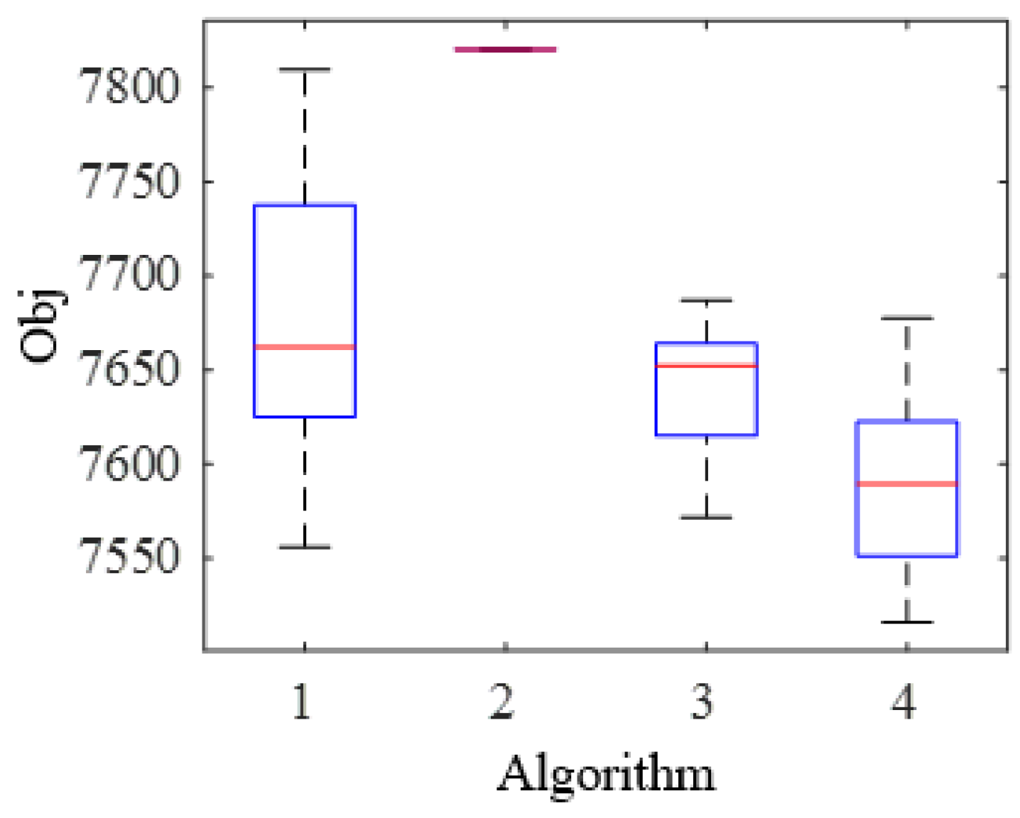
4.3. Comparison of the Components on QL-AO

The proposed QL-AO includes the following key components: (1) NEH heuristic method for initialization, (2) Q-learning-based strategies selection, and (3) local search strategies. To illustrate the performance of each component, we compared the QL-AO without them separately, as shown in Table 4. Each algorithm runs 20 times on a large-scale instances with 100 jobs and 3 machines.
The boxplots of result are shown in Figure 4. It can be seen that the algorithm without heuristic initialization and without local search strategies easily fall into a poor solution. The QL-based strategies selection can significantly improve AO. Other than that, in order to illustrate the probabilities adjustment process, the probabilities curves (Figure 5) were printed out. It can be seen that the selection probabilities of different update strategies are continuously adjusted to find the optimal value.

4.4. Algorithm Comparison

To verify the effectiveness of the proposed QL-AO, it is compared with the most classic algorithms, GA and PSO, three novel algorithms, ABC, CS and JAYA, and the basic AO. In addition, Q-learning-based genetic algorithm (QL-GA) and Q-learning-based artificial bee colony algorithm (QL-ABC), proposed by Chen et al. [35] in 2020 and Long et al. [36] in 2022, respectively, are selected as comparison algorithms. In fairness, the competitive algorithms used the same heuristic initialization method as QL-AO. In addition, ABC, QL-ABC, PSO, CS, JAYA and AO used the same encoding method and local search strategies as QL-AO, and GA, QL-GA used the local search strategies of QL-AO as the mutation part.
Table 5 shows the results of QL-AO and its comparative algorithms on Taillard benchmark where Min, Mean, Std., respectively, indicates the best solution, the mean value, the standard deviation of 20 runs. The minimums of the mean and the min for each instance are bolded. In addition, Wilcoxon test was used to show the significance of the difference between QL-AO and the competitive algorithms. The symbol “+” indicates that QL-AO is significantly better than the competitive algorithm, the symbol “−” indicates that QL-AO is significantly worse than the competitive algorithm, and the symbol “≈” indicates that the difference with the competitive algorithm is not significant under the Wilcoxon rank sum test (α = 0.05). The symbol “+/≈/−” indicates the number of instances that QL-AO is better, similar or worse than the competitive algorithms under the Wilcoxon test.
It can be seen from the data in Table 5 that the mean value of QL-AO is always better than that of AO, and it is significant on large-scale cases. This proves the effectiveness of combining QL and AO. GA, QL-GA, ABC, QL-ABC PSO, CS, and JAYA have excellent performance than QL-AO, respectively, on the small-scale instances 1–4. However, they do not do well on other instances. The reason may be that small-scale instances are not hard, and other algorithms such as CS with strong exploration mechanism may be more appropriate. Further, it is observed that QL-AO always obtains best mean value and best min value on the other larger scale instances 5–12, and it is significant under the Wilcoxon test on instances 7–11. It shows that QL-AO exploitation and exploration abilities have been well balanced by adjusting selection probabilities during the search process compared to other competitors. It can be noted that two advanced algorithms with the involvement of QL, QL-GA and QL-ABC, have certain improvements compared to the basic algorithms GA and ABC, respectively. These are due to the dynamic adjustment of GA’s parameters by QL and dynamic control of ABC’s search dimensions by QL, respectively. However, under this integration optimization issue they still have certain gaps compared to QL-AO and need further improvement.
Figure 6 and Figure 7 separately show the boxplots of optimal solutions and the convergence curves of algorithms on instances 8–9, respectively. It can be concluded that the solution distribution of QL-AO is significantly better than other algorithms and it converges faster.
In order to further verify the performance of QL-AO on more hard instances, we selected seven large-scale instances to test. They are from Ruiz’s new hard benchmark. The results of each algorithm are shown in Table 6.
From Table 6, it is obvious that the proposed QL-AO is clearly better and more effective than other comparison algorithms on the hard instances. It can be concluded that the proposed QL-AO is a new efficient algorithm to solve the integrated scheduling of blocking flowshop.

5. Conclusions

This study investigates the application of a Q-learning-based aquila optimizer (QL-AO) for the integrated optimization problem of blocking flowshop scheduling and preventive maintenance. This QL-AO algorithm can adjust the population update operations during the iteration process adaptively by using Q-learning to update the selection probabilities of four update strategies in the basic aquila optimizer. In addition, an NEH based initialization scheme and five local search methods are employed to further improve the performance of QL-AO. Based on a series of numeric experiments that are carried out on two groups of flowshop scheduling benchmark, this QL-AO algorithm performs significantly better than the other eight comparison algorithms in most test instances. Experimental results also indicate that the proposed Q-learning and local search strategies do well in improving the performance of aquila optimizer for the investigated integrated scheduling problem.
However, there are also some limitations of this study. In terms of modeling, the uncertainty of machine maintenance time, jobs’ arrival time and jobs’ processing time are not taken into account. And this study is conducted without using actual factory data. In terms of algorithm, this study adopts a weighted approach to deal with multi-objective problems, thus unable to obtain non-dominated optimal solutions. In future research, the following topics will be considered. The first straightforward work is to examine the validity of QL-AO in solving the real-world scenarios considering that the test instances are generated from the general flowshop scheduling benchmark in this paper. The second is the design of a Pareto-based multi-objective AO to obtain a non-dominated set for multi-objective optimization. Moreover, it is also interesting to apply Q-learning to determine how to balance the exploration and exploitation period in the aquila optimizer.

Author Contributions

Writing—original draft preparation, Software, Z.G.; Supervision, H.W. All authors have read and agreed to the published version of the manuscript.

Funding

This research is partially supported by the National Science Foundation of China under Grant Nos. 61973203 and 72271048.

Data Availability Statement

Taillard benchmark: http://mistic.heig-vd.ch/taillard/problemes.dir/ordonnancement.dir/ordonnancement.html, (accessed on 15 August 2023). Ruiz’s hard benchmark: http://soa.iti.es/problem-instances, (accessed on 15 August 2023).

Conflicts of Interest

The authors declare no conflict of interest.

References

  1. Azimpoor, S.; Taghipour, S.; Farmanesh, B.; Sharifi, M. Joint Planning of Production and Inspection of Parallel Machines with Two-phase of Failure. Rellab. Eng. Syst. Saf. 2022, 217, 108097. [Google Scholar] [CrossRef]
  2. Ben Ali, M.; Sassi, M.; Gossa, M.; Harrath, Y. Simultaneous scheduling of production and maintenance tasks in the job shop. Int. J. Prod. Res. 2011, 49, 3891–3918. [Google Scholar] [CrossRef]
  3. Basri, E.I.; Abdul Razak, I.H.; Ab-Samat, H.; Kamaruddin, S. Preventive Maintenance (PM) planning: A review. J. Qual. Maint. Eng. 2017, 23, 14. [Google Scholar] [CrossRef]
  4. Wang, H.; Yan, Q.; Zhang, S. Integrated scheduling and flexible maintenance in deteriorating multi-state single machine system using a reinforcement learning approach. Adv. Eng. Inform. 2021, 49, 101339. [Google Scholar] [CrossRef]
  5. Yan, Q.; Wang, H.; Wu, F. Digital twin-enabled dynamic scheduling with preventive maintenance using a double-layer Q-learning algorithm. Comput. Oper. Res. 2022, 144, 105823. [Google Scholar] [CrossRef]
  6. Liu, L.X.; Shi, L.Y. Automatic Design of Efficient Heuristics for Two-Stage Hybrid Flow Shop Scheduling. Symmetry 2022, 14, 162. [Google Scholar] [CrossRef]
  7. Merchan, A.F.; Maravelias, C.T. Preprocessing and tightening methods for time-indexed chemical production scheduling models. Comput. Chem. Eng. 2016, 84, 516–535. [Google Scholar] [CrossRef]
  8. Gong, H.; Tang, L.; Duin, C.W. A two-stage flow shop scheduling problem on a batching machine and a discrete machine with blocking and shared setup times. Comput. Oper. Res. 2010, 37, 960–969. [Google Scholar] [CrossRef]
  9. Elmi, A.; Topaloglu, S. A scheduling problem in blocking hybrid flow shop robotic cells with multiple robots. Comput. Oper. Res. 2013, 40, 2543–2555. [Google Scholar] [CrossRef]
  10. Miyata, H.H.; Nagano, M.S. The blocking flow shop scheduling problem: A comprehensive and conceptual review. Expert. Syst. Appl. 2019, 137, 130–156. [Google Scholar] [CrossRef]
  11. Graham, R.L.; Lawler, E.L.; Lenstra, J.K.; Kan, A.H.G.R. Optimization and approximation in deterministic sequencing and scheduling: A survey. ADM 1979, 5, 287–326. [Google Scholar]
  12. Hall, N.G.; Sriskandarajah, C. A survey of machine scheduling problems with blocking and no-wait in process. Oper. Res. 1996, 44, 510–525. [Google Scholar] [CrossRef]
  13. Jiang, J.; An, Y.; Dong, Y.; Hu, J.; Li, Y.; Zhao, Z. Integrated optimization of non-permutation flow shop scheduling and maintenance planning with variable processing speed. Reliab. Eng. Syst. Saf. 2023, 234, 109143. [Google Scholar] [CrossRef]
  14. Caraffa, V.; Ianes, S.; Bagchi, T.P.; Sriskandarajah, C. Minimizing makespan in a blocking flowshop using genetic algorithms. Int. J. Prod. Econ. 2001, 70, 101–115. [Google Scholar] [CrossRef]
  15. Liang, J.J.; Pan, Q.K.; Chen, T.J.; Wang, L. Dynamic Multi-swarm Particle Swarm Optimizer for blocking flow shop scheduling. In Proceedings of the IEEE International Conference on Fuzzy Systems, Changsha, China, 23–26 September 2010. [Google Scholar]
  16. Li, M.B.; Xiong, H.; Lei, D.M. An Artificial Bee Colony with Adaptive Competition for the Unrelated Parallel Machine Scheduling Problem with Additional Resources and Maintenance. Symmetry 2022, 14, 1380. [Google Scholar] [CrossRef]
  17. Liu, H.; Zhang, X.; Zhang, H.; Li, C.; Chen, Z. A reinforcement learning-based hybrid Aquila Optimizer and improved Arithmetic Optimization Algorithm for global optimization. Expert. Syst. Appl. 2023, 224, 119898. [Google Scholar] [CrossRef]
  18. Ait-Saadi, A.; Meraihi, Y.; Soukane, A.; Ramdane-Cherif, A.; Gabis, A.B. A novel hybrid Chaotic Aquila Optimization algorithm with Simulated Annealing for Unmanned Aerial Vehicles path planning. Comput. Electr. Eng. 2022, 104, 108461. [Google Scholar] [CrossRef]
  19. Bas, E. Binary Aquila Optimizer for 0–1 knapsack problems. Eng. Appl. Artif. Intel. 2023, 118, 105592. [Google Scholar] [CrossRef]
  20. Agarwal, N.; Gokilavani, M.; Nagarajan, S.; Saranya, S.; Alsolai, H.; Dhahbi, S.; Abdelaziz, A.S. Intelligent aquila optimization algorithm-based node localization scheme for wireless sensor networks. CMC-Comput. Mater. Con. 2023, 74, 141–152. [Google Scholar] [CrossRef]
  21. Li, R.; Zhang, X.; Jiang, L.; Yang, Z.; Guo, W. An adaptive heuristic algorithm based on reinforcement learning for ship scheduling optimization problem. Ocean. Coast. Manage. 2022, 230, 106375. [Google Scholar] [CrossRef]
  22. Mao, J.; Hu, X.L.; Pan, Q.K.; Miao, Z.; Tasgetiren, M.F. An improved discrete artificial bee colony algorithm for the distributed permutation flowshop scheduling problem with preventive maintenance. In Proceedings of the 39th Chinese Control Conference, Shenyang, China, 27–29 July 2020. [Google Scholar]
  23. Cheng, L.; Tang, Q.; Zhang, L.; Meng, K. Mathematical model and enhanced cooperative co-evolutionary algorithm for scheduling energy-efficient manufacturing cell. J. Clean. Prod. 2021, 326, 129248. [Google Scholar] [CrossRef]
  24. Zhang, Z.; Tang, Q. Integrating preventive maintenance to two-stage assembly flow shop scheduling: MILP model, constructive heuristics and meta-heuristics. Flex. Serv. Manuf. J. 2022, 34, 156–203. [Google Scholar] [CrossRef]
  25. Sun, L.H.; Ge, C.C.; Zhang, W.; Wang, J.B.; Lu, Y.Y. Permutation flowshop scheduling with simple linear deterioration. Eng. Optim. 2019, 51, 1281–1300. [Google Scholar] [CrossRef]
  26. Wang, S.; Liu, M. Two-machine flow shop scheduling integrated with preventive maintenance planning. Int. J. Syst. Sci. 2016, 47, 672–690. [Google Scholar] [CrossRef]
  27. Ruiz, R.; García-Díaz, J.C.; Maroto, C. Considering scheduling and preventive maintenance in the flowshop sequencing problem. Comput. Oper. Res. 2007, 34, 3314–3330. [Google Scholar] [CrossRef]
  28. Grabowski, J.; Pempera, J. The permutation flow shop problem with blocking. A tabu search approach. Omega 2007, 35, 302–311. [Google Scholar] [CrossRef]
  29. Abualigah, L.; Yousri, D.; Abd Elaziz, M.; Al-Qaness, M.A.; Gandomi, A.H. Aquila optimizer: A novel meta-heuristic optimization algorithm. Comput. Ind. Eng. 2021, 157, 107250. [Google Scholar] [CrossRef]
  30. Bean, J.C. Genetic algorithms and random keys for sequencing and optimization. ORSA J. Comput. 1994, 6, 154–160. [Google Scholar] [CrossRef]
  31. Yang, X.S. Swarm intelligence based algorithms: A critical analysis. Evol. Intell. 2014, 7, 17–28. [Google Scholar] [CrossRef]
  32. Wineberg, M.; Oppacher, F. The underlying similarity of diversity measures used in evolutionary computation. In Proceedings of the Genetic and Evolutionary Computation Conference, Chicago, IL, USA, 12–16 July 2003. [Google Scholar]
  33. Taillard, E. Benchmarks for basic scheduling problems. Eur. J. Oper. Res. 1993, 64, 278–285. [Google Scholar] [CrossRef]
  34. Vallada, E.; Ruiz, R.; Framinan, J. New hard benchmark for flowshop scheduling problems minimising makespan. Eur. J. Oper. Res. 2017, 240, 666–677. [Google Scholar] [CrossRef]
  35. Chen, R.; Yang, B.; Li, S. A Self-Learning Genetic Algorithm based on Reinforcement Learning for Flexible Job-shop Scheduling Problem. Comput. Ind. Eng. 2020, 149, 106778. [Google Scholar] [CrossRef]
  36. Long, X.; Zhang, J.; Zhou, K. Dynamic Self-Learning Artificial Bee Colony Optimization Algorithm for Flexible Job-Shop Scheduling Problem with Job Insertion. Processes 2022, 10, 571. [Google Scholar] [CrossRef]
Figure 1. Diagram of blocking flowshop integrated scheduling.
Symmetry 15 01600 g001
Figure 2. The flow chart of QL-AO.
Symmetry 15 01600 g002
Figure 3. Main effect plots of key parameters. (a) Small-scale instance with 20 jobs and 20 machines; (b) large-scale instance with 400 jobs and 20 machines; (c) large-scale instance with 400 jobs and 20 machines.
Symmetry 15 01600 g003
Figure 4. Boxplots of components comparison.
Symmetry 15 01600 g004
Figure 5. Probabilities adjusting process.
Symmetry 15 01600 g005
Figure 6. Boxplots of optimal solutions.
Symmetry 15 01600 g006
Figure 7. Convergence curves of algorithms.
Symmetry 15 01600 g007
Table 1. States definition table.
StateDescriptionStateDescription
1 c b a d < c 1 & &   p o p d i v < d 1 7 c 1 c b a d < c 2 & &   d 2 p o p d i v < d 3
2 c b a d < c 1 & &   d 1 p o p d i v < d 2 8 c 1 c b a d < c 2 & &   p o p d i v d 3
3 c b a d < c 1 & &   d 2 p o p d i v < d 3 9 c b a d c 2 & &   p o p d i v < d 1
4 c b a d < c 1 & &   p o p d i v d 3 10 c b a d c 2 & &   d 1 p o p d i v < d 2
5 c 1 c b a d < c 2 & &   p o p d i v < d 1 11 c b a d c 2 & &   d 2 p o p d i v < d 3
6 c 1 c b a d < c 2 & &   d 1 p o p d i v < d 2 12 c b a d c 2 & &   p o p d i v d 3
Table 2. Orthogonal experiment settings of QL-AO.
Trial
Number
Factor LevelsRV
(20 × 20)
RV
(5 × 100)
RV
(400 × 20)
n ν δ α γ
1200.10.10.10.52919.897607.1254201.77
2200.30.30.20.62914.637602.1454207.26
3200.50.50.30.72928.077617.9854208.93
4200.70.70.40.82952.317602.1754208.01
5200.90.90.50.92914.067605.1054205.58
6400.10.30.30.82916.637577.4954150.14
7400.30.50.40.92933.997602.0454134.41
8400.50.70.50.52910.077590.7654137.54
9400.70.90.10.62904.777597.7954112.47
10400.90.10.20.72907.467572.7754102.59
11600.10.50.50.62913.427555.6054114.38
12600.30.70.10.72921.557570.6754092.44
13600.50.90.20.82900.787580.5354104.55
14600.70.10.30.92910.337570.7954076.38
15600.90.30.40.52905.617583.0854103.36
16800.10.70.20.92918.757574.1954081.89
17800.30.90.30.52902.097566.8954084.02
18800.50.10.40.62928.777532.7454061.93
19800.70.30.50.72893.977574.9954061.09
20800.90.50.10.82910.997563.4954098.52
211000.10.90.40.72906.507565.4654075.70
221000.30.10.50.82904.087573.8354088.92
231000.50.30.10.92900.067560.3554070.07
241000.70.50.20.52894.667576.2054040.78
251000.90.70.30.62901.787583.8254031.82
Table 3. Response and rank of parameters.
(a) Small-scale instances with 20 jobs and 20 machines
Levels n ν δ α γ
12925.792915.042914.112911.452906.46
22914.582915.272906.182907.262912.67
32910.342913.552916.232911.782911.51
42910.912911.212920.892925.442916.96
52901.422907.982905.642907.122915.44
Delta24.387.2915.2518.3210.49
Rank15324
(b) Medium-scale instances with 100 jobs and 5 machines
Levels n ν δ α γ
17606.907575.977571.457579.887584.81
27588.177583.117579.617581.177574.42
37572.137576.477583.067583.397580.37
47562.467584.397584.327577.107579.50
57571.937581.657583.157580.067582.49
Delta44.448.4212.876.3010.39
Rank14253
(c) Large-scale instances with 400 jobs and 20 machines
Levels n ν δ α γ
154206.3154124.7854106.3254115.0554113.49
254127.4354121.4154118.3854107.4154105.57
354098.2254116.6054119.4054110.2654108.15
454077.4954099.7554110.3454116.6854130.03
554061.4654108.3754116.4654121.5054113.67
Delta144.8525.0313.0914.0924.46
Rank12543
Table 4. QL-AO with different components.
AlgorithmDescription
1QL-AO without NEH heuristic method for initialization
2QL-AO without local search strategies
3QL-AO without QL based strategies selection
4QL-AO with all components
Table 5. Experimental results on Taillard benchmark.
Instance n × m GAQL-GAABCQL-ABCPSOCSJAYAAOQL-AO
120 × 5Min1383.401380.551390.951382.091381.781384.421374.931406.071387.86
Mean1417.191411.311405.281398.081415.451402.321401.291422.981416.74
Std.16.2316.3210.437.8118.7610.8013.0415.4117.57
Wilcoxon
220 × 10Min1904.791906.181912.581910.901938.961913.571910.491912.151917.31
Mean1935.601934.501943.501933.691971.931933.881953.811944.881942.31
Std.22.7721.1213.2611.9822.5517.7821.8322.8222.41
Wilcoxon++
320 × 20Min2845.922844.012836.832828.022866.882824.592851.642875.422881.18
Mean2935.252931.722879.172870.142901.162869.032883.962926.002925.85
Std.50.5339.0918.8618.9722.4224.1520.8136.5131.86
Wilcoxon
450 × 5Min3576.513528.833683.863642.643544.323581.383652.113494.773488.32
Mean3612.923611.973733.723704.983682.183657.063723.943564.163549.49
Std.33.4833.2231.2131.9350.0027.9731.7034.5338.09
Wilcoxon+++++++
520 × 9Min4794.764762.254845.854788.664752.504733.644846.584793.124752.44
Mean4855.404851.914912.504871.814878.564832.864923.754837.014824.00
Std.33.5840.5130.5635.1474.3749.6835.3329.0939.16
Wilcoxon++++++
650 × 10Min7044.377033.187149.357099.147026.407020.967052.657003.966963.96
Mean7105.987094.317195.917159.997147.397114.707185.127076.007067.55
Std.36.5634.6930.6632.8453.8939.9043.0933.7242.41
Wilcoxon+++++++
750 × 20Min7644.537638.807811.627820.397747.917693.947820.397581.377495.38
Mean7710.227708.417819.697820.397816.777796.977820.397628.437598.21
Std.32.9127.532.170.0016.2132.510.0029.7941.21
Wilcoxon++++++++
8100 × 5Min9997.279980.7910,258.1110,233.1310,121.0310,164.8210,188.479920.429885.14
Mean10,079.7510,076.8410,259.7810,256.9110,252.4610,223.5010,255.1710,003.379957.90
Std.67.1457.670.486.4430.9829.4916.1836.8748.03
Wilcoxon++++++++
9100 × 10Min13,518.9513,513.6413,680.8313,602.6013,507.9013,616.9113,621.3813,473.7813,378.77
Mean13,614.5113,611.8713,719.7713,711.6913,683.2913,677.1713,718.2213,530.6813,497.21
Std.43.9542.7827.6635.8873.0233.3632.9226.2744.54
Wilcoxon++++++++
10100 × 20Min19,667.65 19,625.42 19,909.16 19,883.45 19,893.75 19,799.03 19,914.51 19,564.39 19,498.81
Mean19,759.66 19,755.36 19,914.25 19,909.61 19,913.48 19,861.52 19,914.51 19,644.18 19,588.10
Std.51.08 57.72 1.20 8.54 4.64 28.32 0.00 41.36 60.49
Wilcoxon++++++++
11200 × 20Min26,753.76 26,713.04 26,989.87 26,956.33 27,008.19 26,821.13 27,008.19 26,586.15 26,577.62
Mean26,839.01 26,823.55 27,006.69 26,997.57 27,008.19 26,919.17 27,008.19 26,719.92 26,652.97
Std.61.16 68.51 4.73 16.39 0.00 43.78 0.00 51.97 45.25
Wilcoxon++++++++
12500 × 20Min67,501.67 67,498.71 67,629.04 67,620.43 67,629.04 67,483.90 67,629.04 67,350.62 67,327.82
Mean67,582.04 67,575.48 67,629.04 67,628.42 67,629.04 67,566.84 67,629.04 67,465.49 67,444.82
Std.35.89 31.59 0.00 2.06 0.0031.350.00 58.41 55.76
Wilcoxon+++++++
Wilcoxon +/≈/−9/3/09/2/19/1/29/1/210/1/18/2/210/0/25/7/0
Table 6. Experimental results on Ruiz’s hard benchmark.
Instance n × m GAQL-GAABCQL-ABCPSOCSJAYAAOQL-AO
13100 × 20Min13,381.89 13,365.69 13,575.12 13,556.27 13,607.59 13,498.32 13,593.09 13,288.05 13,274.52
Mean13,461.01 13,457.96 13,611.66 13,610.96 13,623.99 13,567.71 13,623.36 13,385.36 13,363.48
Std.61.51 53.06 18.02 21.90 3.88 23.06 7.12 52.22 58.06
Wilcoxon++++++++
14200 × 20Min27,058.88 27,084.77 27,335.85 27,296.28 27,367.67 27,204.34 27,363.98 26,959.71 26,904.79
Mean27,172.23 27,167.89 27,374.07 27,370.44 27,377.79 27,264.71 27,377.60 27,058.02 27,013.08
Std.71.05 71.38 12.93 20.342.3836.423.2144.85 49.14
Wilcoxon++++++++
15300 × 20Min40,531.17 40,577.87 40,799.60 40,799.0140,799.60 40,675.93 40,799.60 40,465.17 40,436.82
Mean40,669.81 40,662.84 40,799.60 40,798.5740,799.60 40,729.63 40,799.60 40,564.75 40,515.46
Std.71.38 38.12 0.00 1.130.0027.69 0.00 62.0541.60
Wilcoxon++++++++
16400 × 20Min54,237.72 54,233.34 54,344.92 54,326.63 54,344.92 54,244.88 54,344.92 54,091.23 54,081.69
Mean54,303.77 54,294.36 54,344.92 54,343.62 54,344.92 54,284.78 54,344.92 54,170.96 54,164.14
Std.27.75 26.91 0.00 4.09 0.00 20.88 0.00 47.79 52.33
Wilcoxon+++++++
17500 × 20Min68,420.67 68,410.24 68,640.32 68,623.26 68,640.32 68,451.30 68,640.32 68,297.54 68,282.72
Mean68,562.80 68,531.40 68,640.32 68,638.17 68,640.32 68,544.95 68,640.32 68,418.68 68,399.91
Std.55.42 38.68 0.00 5.17 0.00 37.85 0.00 55.23 58.95
Wilcoxon++++++++
18600 × 20Min81,641.45 81,637.28 81,744.13 81,716.31 81,744.13 81,624.94 81,744.13 81,562.63 81,504.01
Mean81,713.28 81,711.14 81,744.13 81,740.62 81,744.13 81,663.04 81,744.13 81,627.96 81,627.42
Std.23.93 17.62 0.00 8.50 0.00 18.70 0.00 42.29 51.35
Wilcoxon+++++++
19700 × 20Min94,930.95 94,925.6795,010.06 95,003.24 95,010.06 94,830.38 95,010.06 94,853.35 94,841.62
Mean94,975.91 94,971.3595,010.06 95,009.48 95,010.06 94,932.49 95,010.06 94,923.47 94,921.12
Std.20.54 25.090.00 1.83 0.00 35.92 0.00 42.72 37.68
Wilcoxon++++++++
Wilcoxon +/≈/−7/0/07/0/07/0/07/0/07/0/07/0/07/0/05/2/0
Disclaimer/Publisher’s Note: The statements, opinions and data contained in all publications are solely those of the individual author(s) and contributor(s) and not of MDPI and/or the editor(s). MDPI and/or the editor(s) disclaim responsibility for any injury to people or property resulting from any ideas, methods, instructions or products referred to in the content.

