1. Introduction
Community Supported Agriculture (CSA) has boomed owing to the continuous improvement of living standards and the frequent occurrence of food safety crises. CSA represents a form of direct food selling where local farms provide agricultural products directly to community residents [
1]. In the context of CSA, a farm is responsible for all relevant agricultural product supply chain activities, including planting, picking, and distribution. CSA can greatly shorten the time interval between picking and distribution to improve the freshness of fresh agricultural products, satisfying residents’ demand for agricultural products [
2]. Besides, disruptions of the agricultural supply chain are becoming more and more frequent due to COVID-19 and other emergencies. Growing attention has been devoted to localized production, which is one of the characteristics of CSA [
3]. Hence, CSA is developing rapidly all over the world [
4].
Picking and distribution are two highly related activities in CSA [
5,
6]. The former focuses on arranging for workers to pick agricultural products in the field, while the latter aims to deliver picked products to customers without unnecessary delay. Nowadays, a CSA farm mainly arranges picking scheduling based on experience. The distribution is characterized by scattered customer points and strict requirements for timeliness, which leads to an inefficient use of resources and high distribution costs. To date, most studies have focused on the optimization of picking and distribution separately [
7], which can achieve local optimization but fails in achieving global optimization. As we all know, fresh agricultural products are highly sensitive to time, and their freshness will decay exponentially over time after picking [
8]. Generally, it is not suitable to store them in the inventory for a long time, which creates a great deal of challenges to effectively managing the fresh agricultural supply chain. The picked products must be delivered to customers without unnecessary delay to ensure freshness. Therefore, joint scheduling should to be considered to achieve a seamless link between picking and distribution and achieve an overall optimization.
Thus, this work studies the integrated scheduling problem of the picking and distribution of fresh agricultural products with the consideration of minimizing picking and distribution costs as well as maximizing the freshness of the orders. At the picking stage, all products required by customers are picked according to varieties. The customer order may aggregate a variety of agricultural products planted in different blocks of the CSA farm due to different growth conditions. Therefore, in order to improve efficiency, the CSA farm will collect the order information and pick the products according to their varieties. In addition, different fresh agricultural products have different perishability. This work takes into account the differences in perishability that have an impact on joint scheduling. At the distribution stage, the departure of each vehicle from the farm is equal to the picking completion time of the last product in the vehicle’s cargo. To sum up, there are two main contributions.
- (1)
An integrated scheduling problem of the picking and distribution of fresh agricultural products with the consideration of minimizing picking and distribution costs as well as maximizing the freshness of the order is explored in this work. At the picking stage, a variety of agricultural products need to be assigned among multiple picking groups with different picking abilities. Then the orders are delivered to customers without unnecessary delay. A nonlinear mixed-integer programming model is constructed to formulate the problem.
- (2)
A multi-objective multi-population genetic algorithm with local search (MOPGA-LS) is designed. The designed algorithm is compared with three multi-objective optimization algorithms in the literature: the non-dominated sorted genetic algorithm-II (NSGA-Ⅱ) [
9], the multi-objective evolutionary algorithm based on decomposition (MOEA/D) [
10], and the multi-objective evolutionary algorithm based on decomposition that is combined with the bee algorithm (MOEA/D-BA) [
11]. The comparison results demonstrate that the designed algorithm is a superior optimizer for tackling the integrated picking and distribution problem for agricultural products.
The rest of the paper is structured as follows:
Section 2 reviews the relevant literature. In
Section 3, the investigated problem is abstracted into a mathematical model. A multi-objective multi-population genetic algorithm is proposed in
Section 4. The experimental results and analysis are presented in
Section 5. In the end, the conclusion and future research direction are summarized.
2. Literature Review
There are two closely linked activities in the agricultural product supply chain, namely picking and distribution [
12]. Only through joint scheduling can we achieve overall optimization. Next, this paper reviews the relevant literature from four perspectives: picking, distribution, integrated scheduling, and evolutionary algorithms for solving the integrated scheduling problem.
Literature about agricultural product picking is dedicated to harvesting decisions. Ferrer et al. [
13] investigated the optimization of grape harvesting scheduling with the consideration of minimizing the operational cost as well as minimizing the quality loss. Bohle et al. [
14] expanded the research of Ferrer by taking account into the uncertainties. González-Araya et al. [
15] studied the tactical harvest planning of apple orchards, involving the decision about the quantity of resource input and product to be harvested. The objective was to minimize harvesting costs. In their literature review on the supply chain for agricultural products related to crops, Kusumastuti et al. [
16] concentrated on the integration of scheduling for harvesting and processing as well as the challenges of the related inventory control. Gómez-Lagos [
17] proposed a MILP model to help large export companies manage harvest decisions for multiple orchards. This work focuses on the operational decisions in the picking stage, including which product should be picked by which group and the sequence of products in each group.
Fresh agricultural products are perishable, and their value is closely related to their freshness, which requires maximizing product freshness while meeting cost constraints. Thus, we take the features of agricultural products into account in the Vehicle Routing Problem [
18]. Osvald et al. [
19] studied the distribution of fresh vegetables with time windows and time-dependent travel times to reduce decay and distribution costs. Chen et al. [
20] considered production scheduling and vehicle routing with regard to the time windows of perishable food products. The objective was to maximize the profits of the supplier. Song et al. [
21] investigated the distribution of multi-commodity perishable food products while taking consumer satisfaction into account. It is worth mentioning that the vehicles are heterogeneous, involving refrigerated vehicles and general types of vehicles. Wang et al. [
22] investigated the fresh agricultural product distribution route with the consideration of minimizing the time window penalty cost as well as maximizing customer satisfaction. In brief, the balance between cost and freshness is rarely considered in the existing literature.
Recent research has considered the integrated production and distribution scheduling problem (IPDSP) in the perishable products industry. The research of Amorim et al. [
23] showed that the integrated approach can effectively improve the freshness of perishable products. Geismar et al. [
24] studied an IPDSP of a product with short shelf life, where the product was processed at the factory with a single machine and the finished product was delivered to customers before expiration by a truck. The objective was to minimize the overall time. Devapriya et al. [
25] expanded the research of Geismar, considering more realistic features, such as the decision of the fleet size and a planning horizon constraint. The scheduling objective was to minimize the cost. Belo-Filho et al. [
26] studied an IPDSP of perishable products where the customer order with several products could be processed by multiple parallel capacitated production lines. The objective was to minimize the total operating cost through the joint decision. An adaptive large neighborhood search framework was proposed to deal with the problem. Kergosien et al. [
27] investigated the coordinated scheduling of a chemotherapy product in order to decrease the tardiness of delivery. Philippe et al. [
28] studied an IPDSP of a single perishable product and proposed a greedy random adaptive search procedure with an evolutionary local search to solve it. It was designed to minimize the overall time of production and distribution systems. Neves-Moreira [
29] addressed an IPDSP in the meat supply chain, which comprised a single processing center with several production lines and a fleet of vehicles. The scheduling objective was to minimize global costs. By summarizing the above literature, we can find that research on the integrated production and distribution scheduling in the perishable products manufacturing industry has primarily concentrated on the perishability of products, while failing to investigate the fact that different kinds of agricultural products have different decay rates. Therefore, different from the integrated production and distribution scheduling in the manufacturing industry, where products are processed according to customer orders, it is significant to give priority to picking products according to the varieties when a variety of agricultural products with different decay rates are involved.
Evolutionary algorithms based on population are regarded as an effective approach to solving the integrated scheduling problem. Gharaei et al. [
11] presented a novel multi-objective algorithm based on decomposition which had been combined with the bee algorithm (MOEA/D-BA) to solve the integrated scheduling problem in a multi-factory supply chain. Marandi et al. [
30] solved the integrated scheduling problem with four different types of population-based metaheuristics solution approaches, i.e., the Genetic Algorithm, PSO, Improved PSO, and Imperialist Competitive Algorithm. Mohammadi et al. [
31] developed a hybrid particle swarm optimization (HPSO) algorithm to solve the integrated scheduling problem for medium and large sizes. In sum, evolutionary algorithms based on population can effectively solve the integrated scheduling problem in a reasonable time. However, one of the limitations of evolutionary algorithms is that they perform poorly in local search. Thus, it is appropriate to combine the evolutionary algorithm with local search. Qin et al. [
32] developed an improved Particle Swarm Optimization (PSO) algorithm combined with a local optimal solution jumping mechanism to achieve infrared image enhancement. In order to perform the parameter estimation of photovoltaic systems, Tefek M. F. [
33] proposed an ABC-Local Search (ABC-Ls) method by combining the standard artificial bee colony algorithm with a new local search. Ul Hassan N. [
34] proposed an improved opposition-based Particle Swarm Optimization algorithm to balance global and local search, so as to achieve global optimization. Saad et al. [
35] proposed an evolutionary multi-objective artificial bee colony (EMOABC) algorithm incorporating the characteristics of the simulated evolution (SE) algorithm for improved local search. Liu et al. [
36] proposed a modified cuckoo search algorithm with variational parameters and logistic map (VLCS) to avoid falling into a local optimum and improve the rate of convergence. Fu et al. [
37] proposed a new multi-objective brain storm optimization algorithm incorporating a stochastic simulation approach to solve a stochastic multi-objective distributed permutation flow shop scheduling problem. Fu et al. [
38] proposed a multi-objective multiverse optimization algorithm with stochastic simulation to solve a disassembly sequence planning problem with a stochastic bi-objective.
We can conclude from the materials discussed in this section that previous studies have paid little attention to the integrated picking and distribution scheduling of fresh agricultural products, especially when considering a variety of fresh agricultural products with different decay rates. However, overall optimization can only be achieved through integrated scheduling. Meanwhile, owing to the intricacy of the problem under consideration, an efficient tool, namely metaheuristic methods, has been widely employed to cope with them. Thus, this work studies an integrated scheduling problem of the picking and distribution of fresh agricultural products with the consideration of minimizing the picking and distribution costs as well as maximizing the freshness of the orders. Then, a multi-objective multi-population genetic algorithm with local search (MOPGA-LS) is designed to solve this problem.
3. Problem Statement
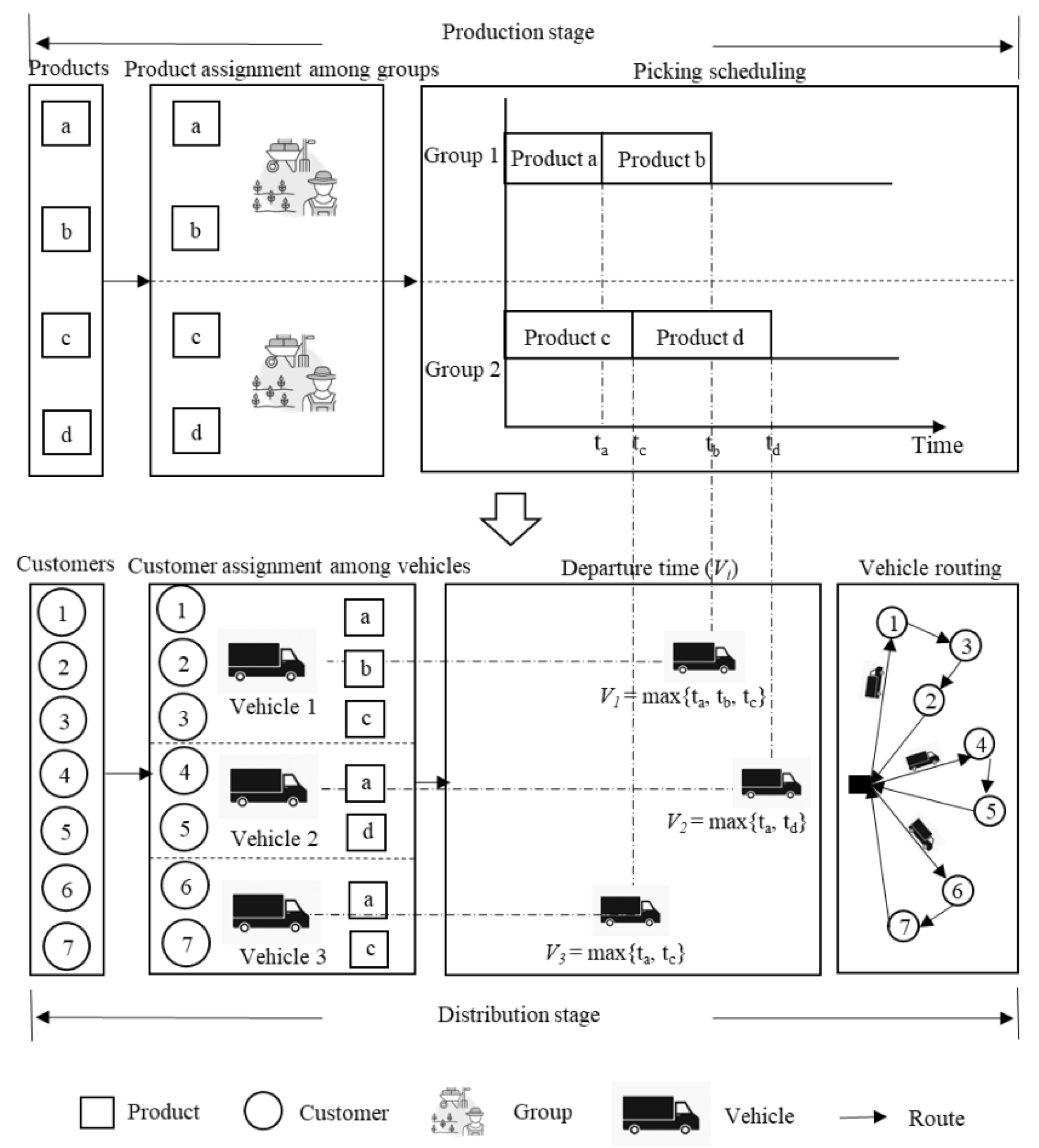
Two pivotal stages are contained in the problem under consideration: the picking stage and the distribution stage. There are multiple picking groups with different picking speeds in the picking stage. A variety of agricultural products must be assigned among groups, and each product may only be assigned to one group. All products assigned to a group are picked by the group following the determined sequence. A group can pick only one product at a time, and interruption is not permitted.
The distribution stage can be abstracted into a vehicle routing problem centered on delivering the orders to the customers, where the vehicles have a defined maximum capacity. The CSA farm should determine how many vehicles to use, the vehicle assignments, and the sequence of customers for each trip. Each customer can only be visited once. Notice that the customer order may aggregate a variety of agricultural products that must be picked separately. Once picked, a product will be loaded into the corresponding vehicle according to the distribution scheduling. Then the departure time of each vehicle from the farm is equal to the picking completion time of the last product in the vehicle’s cargo.
The freshness of agricultural products decays exponentially with time after picking, and different agricultural products decay at different speeds [
39,
40]. Based on the existing research on the freshness function, this work constructs a freshness function:
, where
represents the decay rate of the agricultural product,
represents the time between picking and distribution, and
is a constant. In the considered problem, a variety of agricultural products are divided into two types according to their decay rate. The agricultural products with the decay rate
are more sensitive to time, and the others with the decay rate
are less sensitive to time. An integrated picking and distribution schedule in which a farm serves multiple customers is depicted in
Figure 1.
Table 1 provides the notations and definitions and the mathematical model is established as follows:
s.t
where (1) is to minimize the total cost of picking and distribution. The picking cost mainly contains the labor cost of the picking process, and the distribution cost is made up of both fixed and variable costs. Constraint (2) is to maximize the freshness of all the orders. Constraints (3)–(6) guarantee the order relationship of two adjacent products and that each product should be picked by only one group. Constraint (7) guarantees that a group is allowed to pick only one product at a time and defines the completion time of the products at the picking stage. Constraint (8) specifies that the departure time of each vehicle from the farm is equal to the picking completion time of the last product in the vehicle’s cargo. Constraint (9) denotes that each customer should be assigned to only one vehicle. Constraint (10) restricts each customer in each tour to only one immediate previous customer. Constraint (11) guarantees that the capacity of each vehicle must be met. Constraint (12) specifies that each vehicle starts from the farm and finally returns to it. Constraint (13) indicates a flow balance. Constraint (14) defines the visiting time of customer
by vehicle
. Constraint (15) is employed to eliminate sub-tours in the distribution. Constraints (16) and (17) give the range of variables.
The problem under consideration contains two pivotal types of problem: unrelated parallel machine scheduling and vehicle routing problems. Both of them have proven to be NP-hard, and the considered problem is more complicated because it simultaneously optimizes two conflicting criteria. Consequently, it is also NP-hard, and we propose the MOPGA-LS to deal with it.
4. Proposed Algorithm
Multi-objective optimization problems have multiple Pareto optimal solutions, and the goal of solving them is to find as many Pareto optimal solutions as possible. Evolutionary algorithms can find a set of solutions with a single iteration, and thus they have been popularly regarded as an effective approach to solving multi-objective problems [
41]. Extensive experimental comparisons verify their excellent performance in addressing complicated multi-objective optimization problems [
42]. Motivated by their successful applications, this work proposes the MOPGA-LS to settle the problem under study.
4.1. Solution Representation
To solve the integrated picking and distribution problem, we need to make four decisions, i.e., the product assignment among groups, the picking sequence of the products at the picking stage, the customers served by each of the vehicles, and their delivery routes at the distribution stage. Thus, this work uses an integer string to represent a solution, i.e., a chromosome which consists of three parts. Part
represents the picking sequence, where each integer indicates a product index. Part
denotes the product assignment among groups, where each integer indicates the number of varieties picked by each group. Through parts
and
, we can clearly know which group picks which agricultural product and the picking sequence within each team. As is shown in
Figure 2, group 1 picks two products in the order of product 3 and 6, group 2 picks three products in the order of product 5, 2, and 7, and group 3 picks two products in the order of product 1 and 4. Part
indicates the distribution sequence, where each integer indicates a customer. Notice that Part
just gives the delivery sequence of the customers and fails to provide the customer assignment among vehicles. This work employs a decoding rule for Part
to minimize the number of vehicles [
43]. In this method, the customers are sequentially assigned to a vehicle as their delivery sequence. If the load of a vehicle exceeds the maximum capacity, a new vehicle comes into use.
Figure 2 illustrates the decoding rule. The capacity of the vehicle is set to 6. Thus, vehicle 1 serves customer 4, vehicle 2 severs three customers in the order of customer 3, 2, and 6, and vehicle 3 severs two customers in the order of customer 5 and 1. It is worth mentioning that the above encoding method avoids the generation of infeasible solutions.
4.2. Population Initialization
Two heuristic rules combine with the random generation mode to construct an initial population. This work employs two heuristic rules to generate an individual, which are, respectively, named the Sensitivity Priority Rule and the Mileage Saving Method [
44]. The details are as follows.
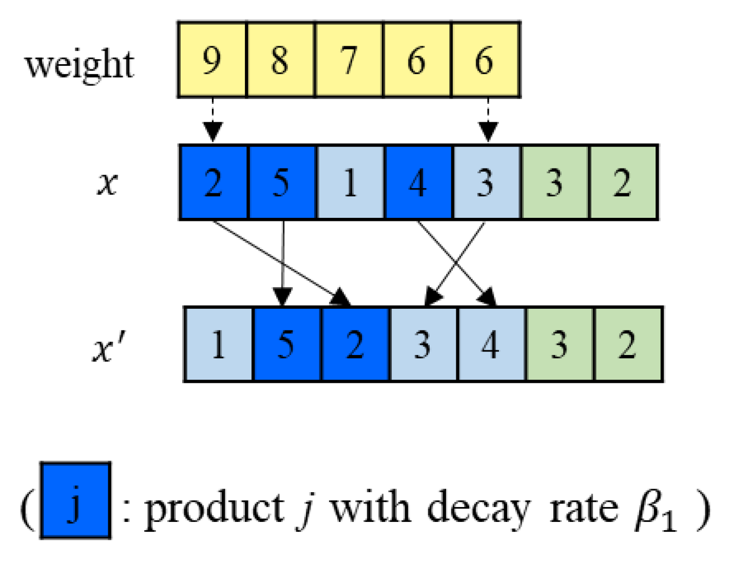
The Sensitivity Priority Rule: In a group, all products are divided into two types
and
according to their decay rate. The products in
are more sensitive to time and are sorted in non-decreasing order according to picking weights. The products in
are less sensitive to time. Then the group first picks the products in
as their original picking sequence, and finally picks the products in
as their sorted sequence. The details are presented in
Figure 3.
The Mileage Saving Method: Its core idea is to generate the initial solution with the shortest total distribution distance under the constraint that the vehicle has the maximum load limit. Its main approach is to make the two loops existing in transport problems and into one loop , reducing the total transport distance.
4.3. Multi-Population Construction
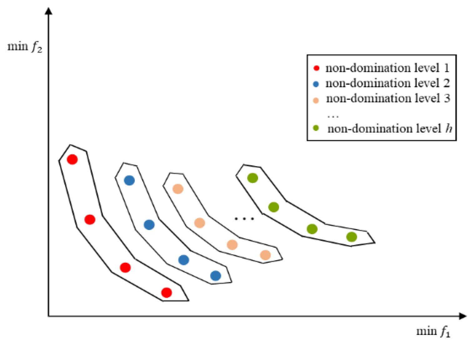
The solutions obtained in this work are called non-dominated solutions, i.e., Pareto solutions, because they simultaneously optimize two conflicting criteria. Thus, Fast Non-dominated Sorting (FNS), a crucial component of NSGA-II, is employed to sort a population into different non-domination levels [
9], as is shown in
Figure 4. The considered problem is designed to minimize the picking and distribution cost and maximize the freshness of the orders. In the process of calculation, we take the reciprocal of the value of the second objective function. Then a population
in MOPGA-LS can be sorted into different non-domination levels
,
,…,
. Based on this, we can perform a global search and local search, respectively, in different non-domination levels, i.e., perform a global search in all non-domination levels and perform a local search in non-domination level 1. Furthermore, the MOPGA-LS utilizes multiple non-domination levels to improve genetic operation. In short, it performs crossover operations on more promising solutions to enhance the algorithm’s efficiency. The details are as follows.
4.4. Selection, Improved Crossover, and Mutation
The selection mechanism is described as follows. Firstly, through the FNS method, the Pareto-based rank and crowding distance are assigned to each individual in the parent population. Then, two individuals are selected randomly from the population every time, and compare their rank values. The individual with a smaller rank value is copied to an offspring. If the rank values of two individuals are the same, the individual with the bigger crowding degree value is copied to the next generation. Finally, repeat the above operations until the offspring population size reaches the original population size.
The individuals in the offspring population can be divided into the multi-population according to the Pareto-based rank. Based on this, MOPGA-LS improves the crossover operation. The following are the specific steps.
Step 1: Determine the non-domination level where the individuals for crossover are located. Randomly generate two integers in , where represents the number of non-domination levels. Then, the smaller integer value represents the non-domination level.
Step 2: Randomly select an individual as one of the parent individuals for crossover in the selected non-domination level.
Step 3: Repeat Steps 2 to 3 to generate another parent individual for crossover.
Step 4: Two parent individuals perform a partially mapped crossover.
The mutation takes place immediately after the improved crossover. A random number in is generated. Perform the mutation operation if the generated number is equal to or smaller than , where represents the mutation probability. The three mutation operations are as follows.
(1) Randomly select a product in Part , delete it from the current location, and then insert it into a location randomly.
(2) Randomly select two points (denoted as ) in Part . If and , then , and ; otherwise, , and .
(3) Randomly select a customer in Part , delete it from the current location, and then insert it to a location randomly.
Finally, the MOPGA-LS forms the next-generation population according to the elite-preservation strategy [
9].
4.5. Local Search
After performing genetic operations, this work refines the non-dominated individuals by using a local search method (LSM) with probability , , where is the current number of function evaluations, and is the maximum number of function evaluations. If a random number is equal to or smaller than , the LSM is allowed to be performed. It uses a colling process like the simulated annealing method to avoid falling into a local optimum. To efficiently use the computation resource, the LSM is allowed to refine individuals at most. Different from other similar works, this work combines a local search with a simulated annealing algorithm to determine the number of neighborhood solutions and maintain the diversity of the neighborhood solutions, so as to avoid falling into local optima and improve the performance of the proposed algorithm.
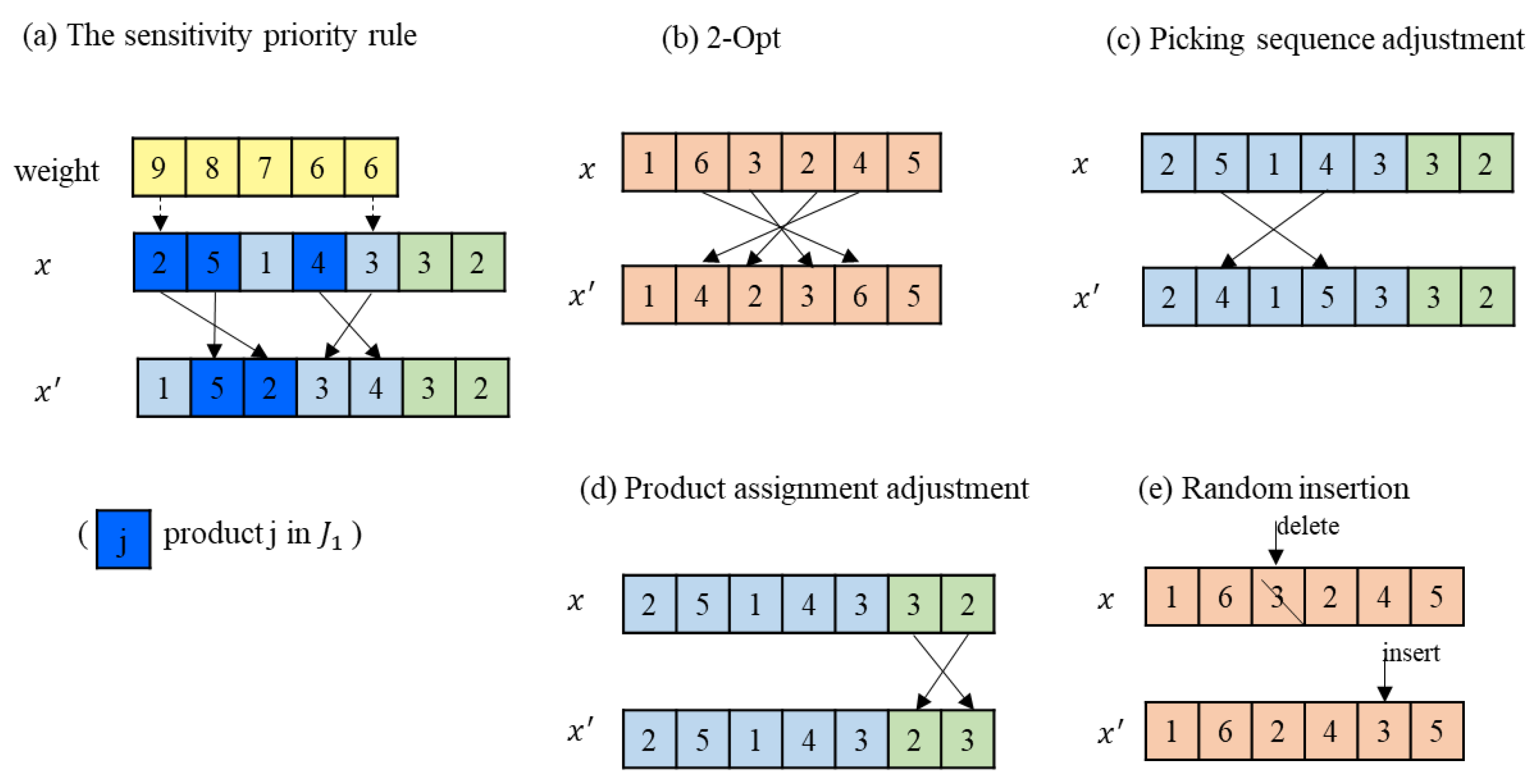
To generate a neighbor individual, this work designs five neighborhood structures as follows, and
Figure 5 illustrates them.
(1) The Sensitivity Priority Rule: The details are described in
Section 4.2.
(2) 2-Opt: Select a segment in Part
of an individual and reverse the segment. A concrete example can be given in
Figure 5, where the segment
in Part
is reversed to
.
(3) Product assignment adjustment: Randomly select two points in Part to exchange.
(4) Picking sequence adjustment: Randomly select two products in Part to exchange.
(5) Random insertion: Randomly select a customer in Part , delete it from the current location, and then insert it to a location randomly.
The metropolis acceptance principle [
45] is adopted to make the LSM jump out of the local optima. It is necessary to calculate the difference between the neighbor solution
and the initial solution
of the first and second objective function values, i.e., ∆1
and ∆2
. In addition,
,
and
are required, where
,
,
is a uniformly distributed random number, and the Boltzmann constant
. Given that a bi-objective is being evaluated, there are five conditions for dealing with the new neighbor solution
:
(1) and : is accepted;
(2) and : is accepted only if ;
(3) and : is accepted only if ;
(4) : is accepted only if ;
(5) : is accepted only if .
The procedures of the LSM are as follows:
Step 1: Initialize the parameters, involving the maximum number of individuals selected for local search , the initial temperature , the final temperature , the coefficient that controls the cooling schedule , and .
Step 2: Select an individual randomly in .
Step 3: Utilize five neighborhoods to create an individual based on . If meets the Metropolis acceptance principle, then
Step 4: .
Step 5: Steps 3 to 4 must be repeated until is reached.
Step 5: If a specified termination criterion is fulfilled, output ; otherwise, go to Step 2.
Step 6: Update the population by selecting individuals in randomly to return.
4.6. Procedure of MOPGA-LS
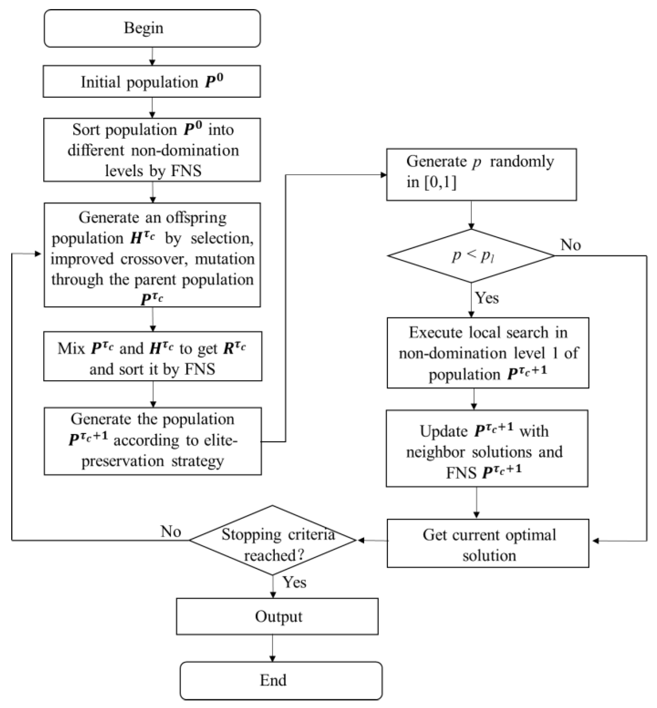
Having discussed the components of MOPGA-LS, we next summarize the concrete steps of MOPGA-LS, which are shown in
Figure 6.
Step 1: Initialize the parameters of MOPGA-LS, such as the population size , the mutation probability , and the maximum number of function evaluations .
Step 2: Initialize the population, calculate the fitness and perform the Fast Non-dominated Sorting.
Step 3: Generate an offspring population by performing genetic operations.
Step 4: Generate a new generation population according to the elite-preservation strategy.
Step 5: If < , refine the non-dominated individuals by using a local search method, and perform the Fast Non-dominated Sorting.
Step 6: If a termination requirement is reached, that is the maximum number of function evaluations, so export non-dominated solutions; otherwise, go to Step 3.
5. Computational Experiments
Experiments are conducted on 32 different sets of benchmark instances. This work selects three multi-objective evolutionary algorithms: NSGA-Ⅱ, MOEA/D, and MOEA/D-BA, as the peer approaches for comparisons. NSGA-Ⅱ and MOEA/D are classic multi-objective evolutionary algorithms that can handle routing planning and job shop scheduling [
46,
47]. MOEA/D-BA is also used to handle the integrated production and distribution scheduling problem that includes two pivotal problems: parallel machine scheduling and vehicle routing problems [
11].
5.1. Test Instance Generation
There are no instances suitable for the problem under consideration, which contains a picking stage and a distribution stage, in the existing literature. Therefore, a set of instances in the picking stage are generated by using the approach described by Belo-Filho [
27], and the distribution stage benchmark may be obtained at
http://www.coin-or.org/SYMPHONY/branchandcut/VRP/data/index.htm.old (accessed on 1 August 2022).
Table 2 outlines the information about the picking groups, mainly involving their unit picking speed and unit picking cost. The unit picking speed follows a uniform distribution and the unit picking cost is a constant. The fixed cost of utilizing each vehicle
is set to 150, the variable cost of the vehicle per unit of time
is set to 1.5, and the vehicle speed is set to 30.
The size of the test instances is determined by four factors, including the number of groups, the number of products with decay rate
, the number of products with decay rate
, and the number of customers. This work tests eight different sizes, and the details are described in
Table 3. There are four instances for each size. Therefore, this work tests a total of 32 instances to evaluate the performance of the algorithm. In the following experiments, each algorithm runs 20 times for each instance, and the mean value is calculated to evaluate its performance. All the algorithms stop when
function evaluations are used up, where
represents the number of groups,
represents the number of products, and
represents the number of customers.
5.2. Performance Metrics
This work selects two performance metrics, i.e., the hypervolume-metric and the IGD-metric, to compare the performance of different algorithms. HV and IGD are by far the most accepted performance metrics, as is proved by Riquelme N. (2015) [
48] et al. In addition, this work utilizes two statistical methods, i.e., a
t-test and a
u-test, to analyze the statistical significance of the results obtained using the MOPGA-LS and the algorithms in the comparison pool. The symbols +, −, and ~ denote statistical results with a significance level of 0.05. The results are given as +, −, or ~ if the MOPGA-LS is significantly better than, significantly worse than, or equivalent to each of the three multi-objective evolutionary algorithms.
(1) The Hypervolume-metric: The HV measures the size of the objective space covered by an approximation set. A reference point must be used to calculate the mentioned covered space. In our experiments, is set to a reference point and all the objective vectors in approximation sets are normalized into [0, 1]. The bigger the HV, the better the obtained non-dominated solution set.
(2) Inverted Generational Distance: IGD calculates the minimum Euclidean distance between an approximation set and the Pareto optimal front. Because the Pareto optimal front of the investigated problem is unknown, the set of non-dominated solutions obtained by the four algorithms in all runs is regarded as the approximate Pareto optimal front, which refers to Saibal Majumder [
49]. The specific steps are as follows.
Step 1: Mix all the solutions obtained by 20 independent executions of each of the algorithms.
Step 2: Perform the Fast Non-dominated Sorting of all the solutions to obtain the set of non-dominated solutions, which is regarded as the approximate Pareto optimal front.
5.3. Parameter Setting
To obtain the optimal parameter combination of the MOPGA-LS, an orthogonal experiment is carried out on the test instance with 3 groups, 15 products with decay rate , 15 products with decay rate , and 40 customers. The population size , the number of individuals selected for local search , the simulated annealing rate , and the number of neighbor solutions selected for return are the four most important parameters influencing algorithm performance. Each parameter has four levels, where ,, , and . Thus, an orthogonal array is selected to carry out the orthogonal experiment. In addition, the mutation rate, the initial temperature , and the final temperature in the MOPGA-LS are set to 0.25, 0.8, and 1500.
This experiment selects the hypervolume-metric as the performance metric [
39]. The bigger the hypervolume, the better the obtained non-dominated solution set. The MOPGA-LS runs 20 times for each parameter combination independently, and the response value (
RV) is calculated according to the average Hypervolume value over 20 independent runs. Additionally, the termination criterion, namely the maximum number of function evaluations, is set to
, where
represents the number of groups,
represents the number of products, and
represents the number of customers. The results of the orthogonal experiment are displayed in
Table 4, and the parameters’ significance rankings are depicted in
Table 5.
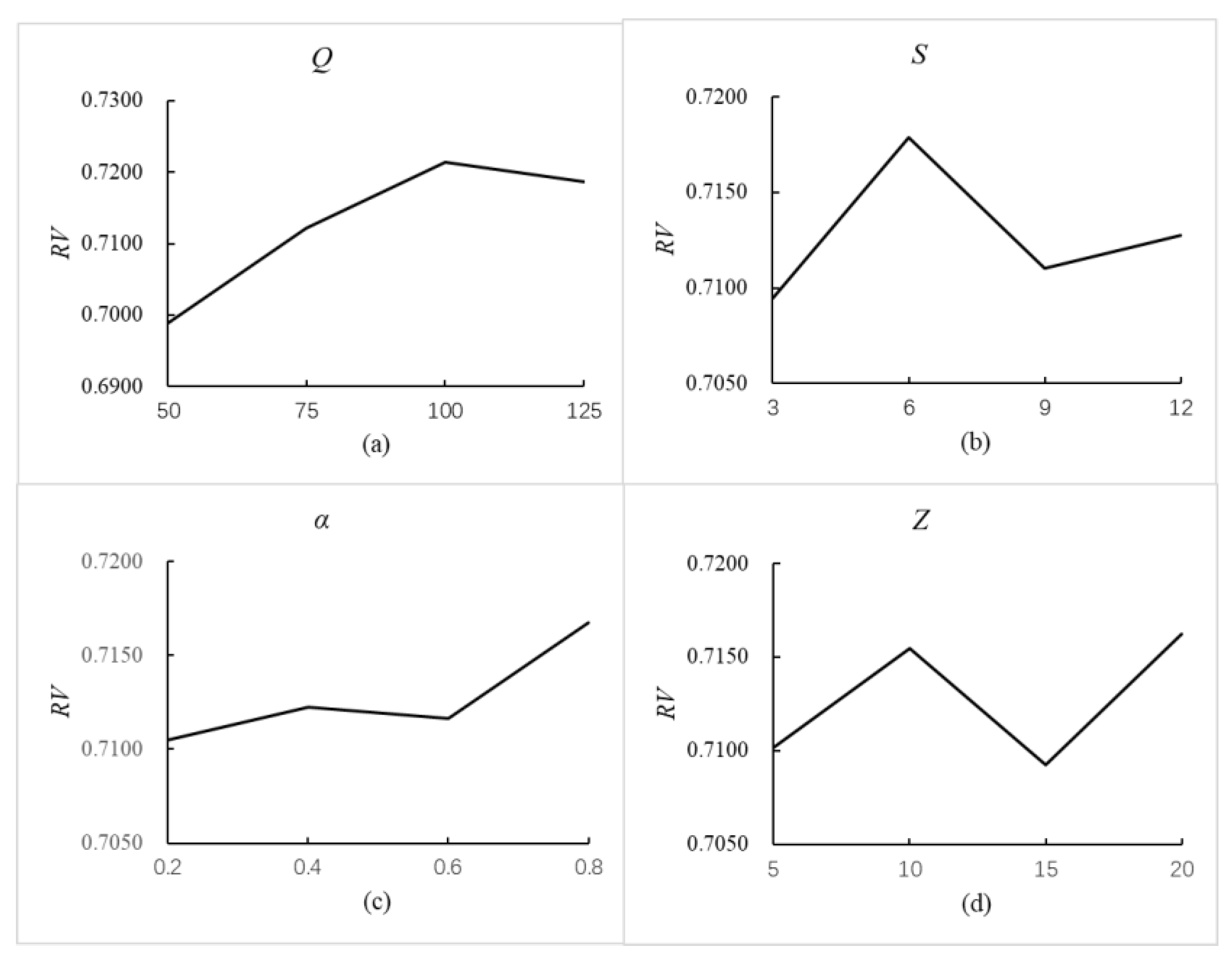
Figure 7 illustrates the factor level trend of each parameter vividly. Based on these findings, we conclude that
is the most important parameter and
has minimal impact on the algorithm’s performance. Therefore, we conclude that, when
and
, the MOPGA-LS performs best.
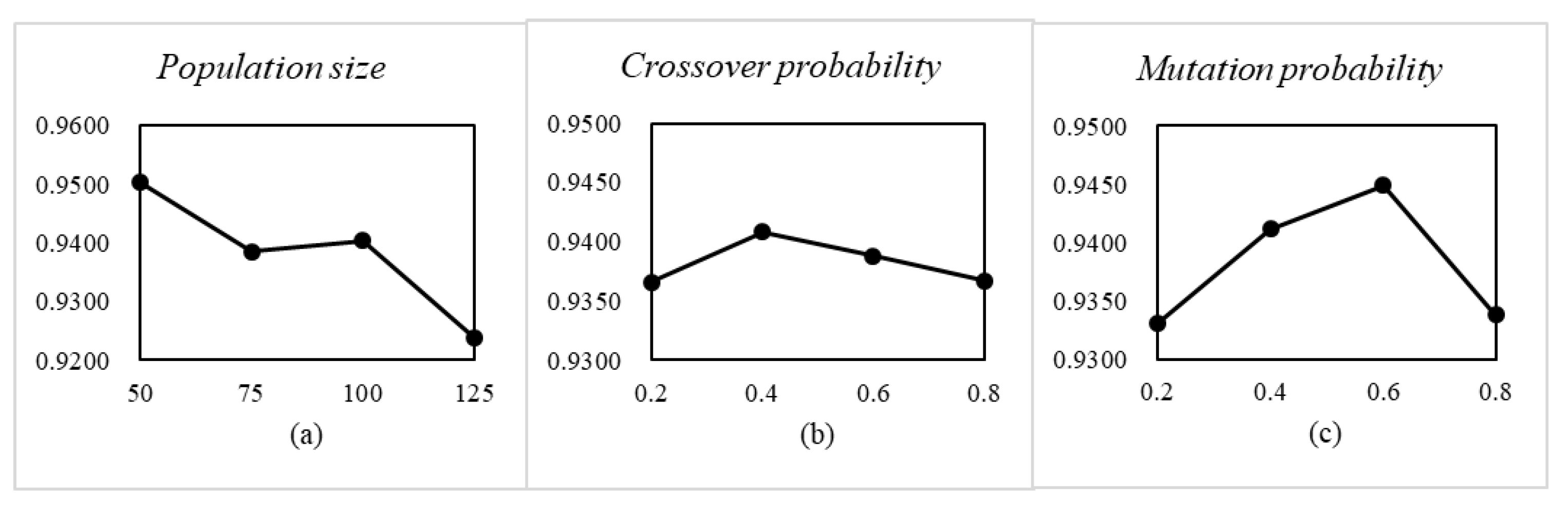
The optimal parameter combination of NSGA-II, MOEA/D, and MOEA/D-BA is also determined by the orthogonal experiment. In NSGA-II, the population size, crossover probability, and mutation probability are the three key parameters. The factor level and the experimental result is shown in
Figure 8. Therefore, we conclude that when the population size
, the crossover probability
, and the mutation probability
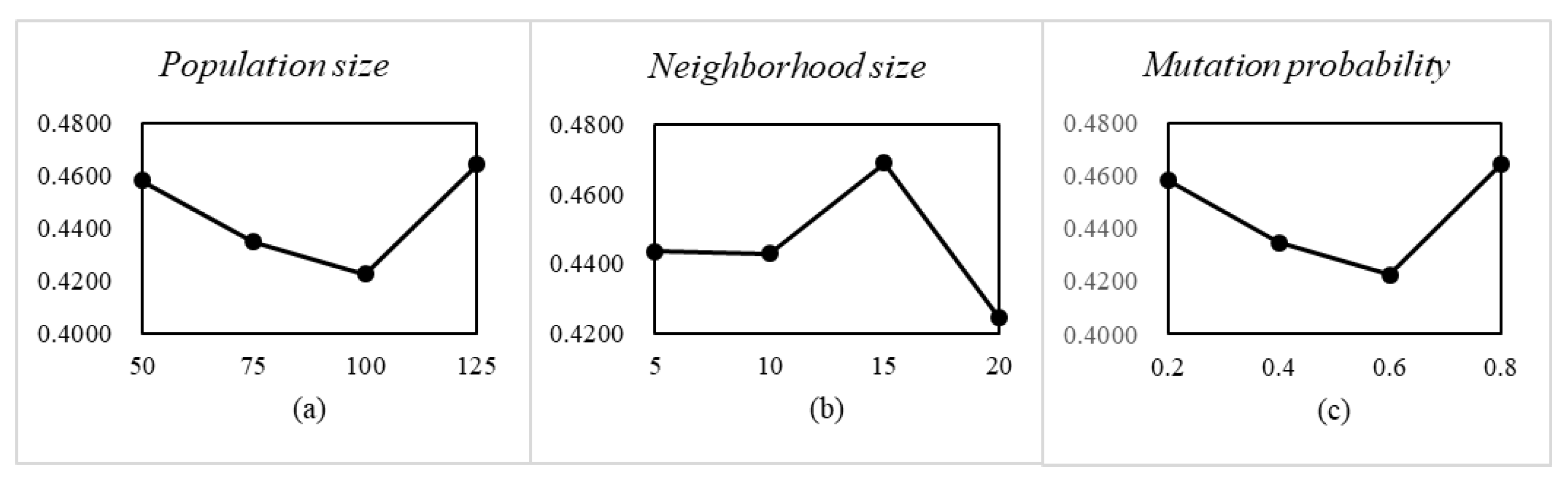
, NSGA-II performs best. In MOEA/D, the population size, neighborhood size, and crossover probability are the three key parameters. The factor level and the experimental result are shown in
Figure 9. Therefore, we conclude that when the population size
, the neighborhood size
, and the crossover probability
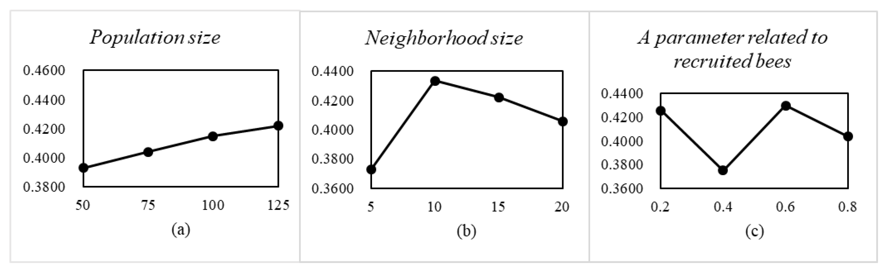
, MOEA/D performs best. In MOEA/D-BA, the population size, neighborhood size, and a parameter related to the number of recruited bees are the three key parameters. The factor level and the experimental result is shown in
Figure 10. Therefore, we conclude that when the population size
, the neighborhood size
, and the parameter related to the number of recruited bees
, MOEA/D-BA performs best.
5.4. Experimental Results
This work makes a comparison among four algorithms in terms of their hypervolume-metric and IGD-metric. The experimental results are as follows.
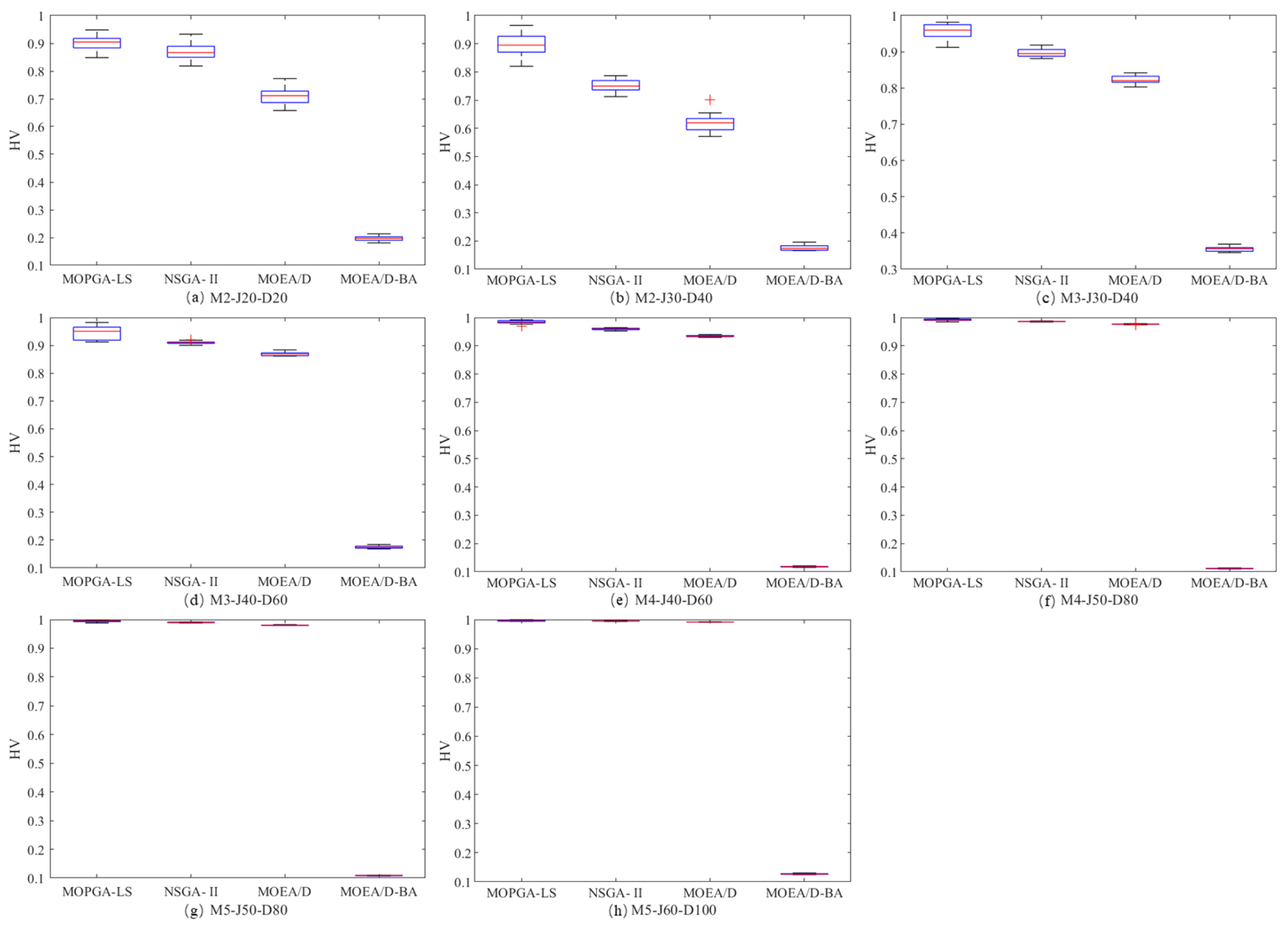
Table 6 shows the average of the HV-metric over 20 independent runs of the four algorithms. Though a
t-test, we can conclude that the MOPGA-LS greatly outperforms NSGA-II in 28 of the 32 test instances, is equivalent to NSGA-II in the other four, and outperforms both MOEA/D and MOEA/D-BA. Though a
U-test, we can conclude that the MOPGA-LS greatly outperforms the NSGA-II in 27 of the 32 test instances, is equivalent to the NSGA-II in the other five, and outperforms both MOEA/D and MOEA/D-BA. In addition, the boxplots of the hypervolume-metric, which vividly show the efficiency of the MOPGA-LS, are shown in
Figure 11.
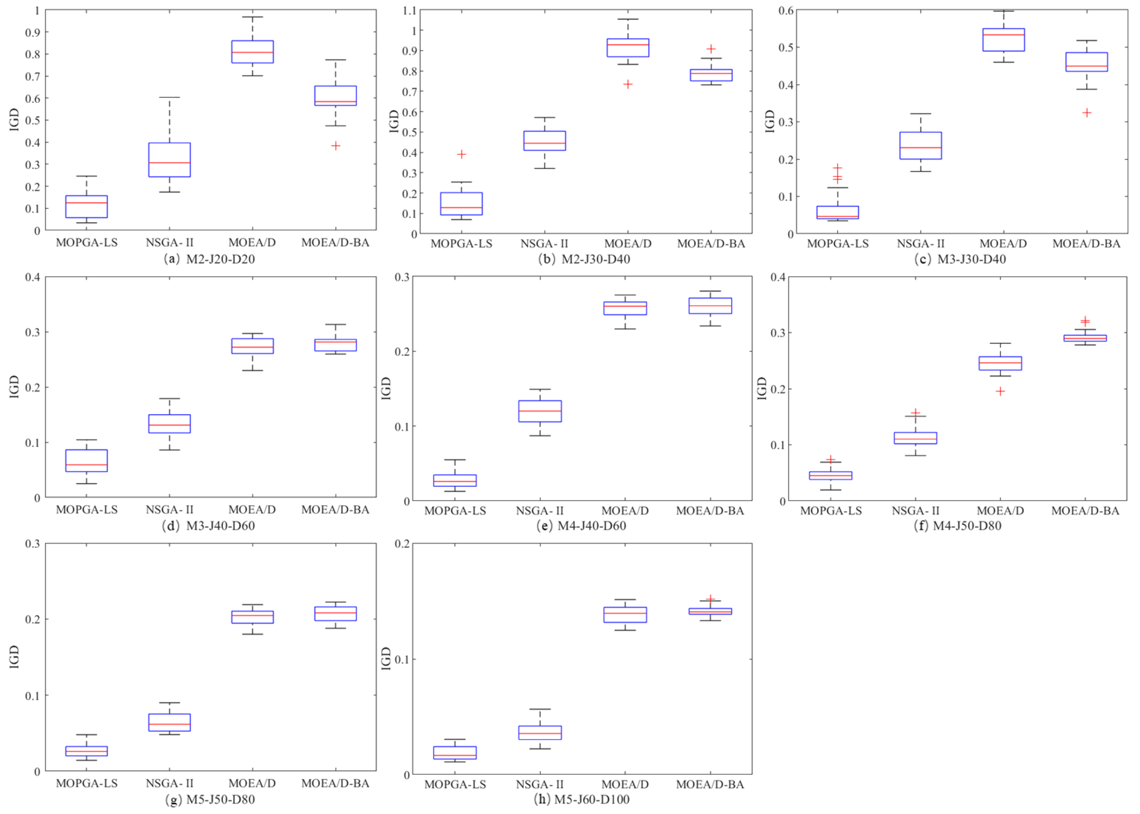
Table 7 shows the average of IGD-metric over 20 independent runs of the four algorithms. The results of the
t-test and
U-test show that the MOPGA-LS outperforms NSGA-II, MOEA/D and MOEA/D-BA. Similarly, the boxplots of the IGD-metric are shown in
Figure 12.
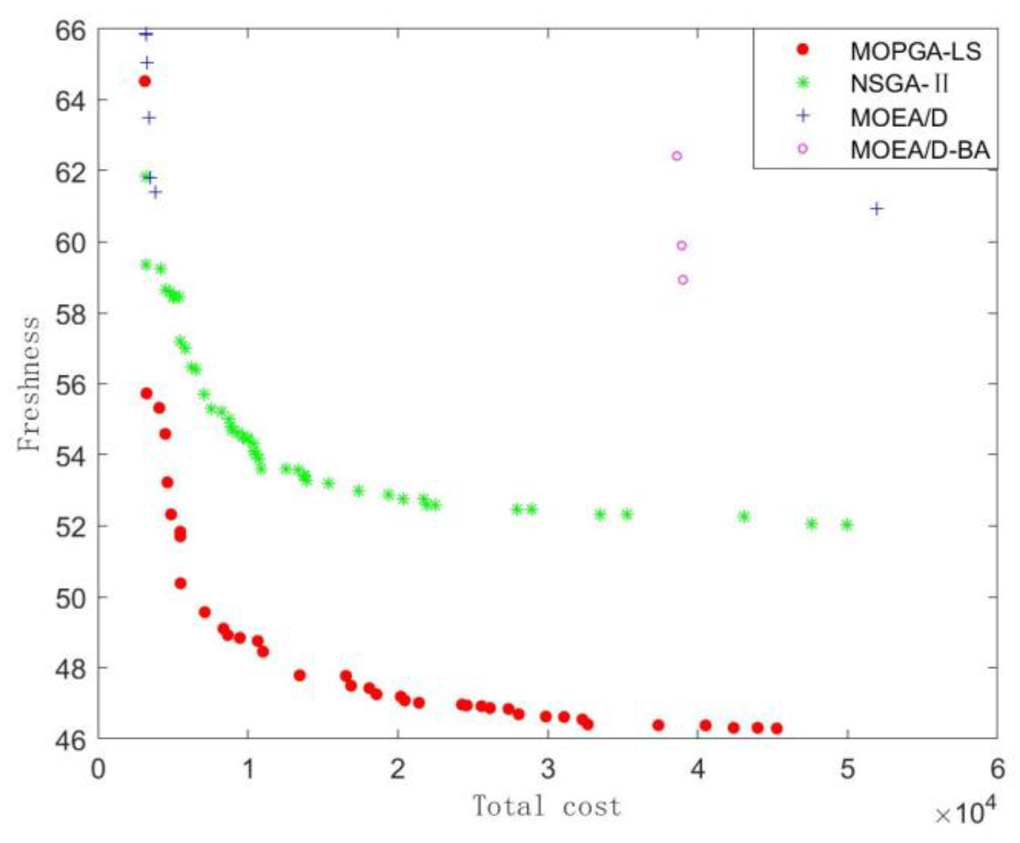
Finally, the distribution of these non-dominated solution sets obtained by the four algorithms in the instance of 3 groups, 15 products with decay rate
, 15 products with decay rate
, and 40 customers is depicted in
Figure 13. It is clear that the solution sets obtained by the MOPGA-LS have superior approximation and distribution to those obtained by the other algorithms. Therefore, we conclude that the proposed algorithm is a superior optimizer for addressing the integrated picking and distribution problem of agricultural products. The experimental results in terms of the hypervolume-metric and IGD-metric show that the MOPGA-LS has better approximation and distribution than other algorithms as peers. The advantages of the MOPGA-LS over NSGA-II, MOEA/D, and MOEA/D-BA illustrate that the multi-population effectively balances the global search and local search. In addition, the improved crossover operation and the combination of local search and the simulated annealing algorithm improve the efficiency of the MOPGA-LS.


