Some Explicit Properties of Frobenius–Euler–Genocchi Polynomials with Applications in Computer Modeling

Abstract

Many properties of special polynomials, such as recurrence relations, sum formulas, and symmetric properties, have been studied in the literature with the help of generating functions and their functional equations. In this study, we define Frobenius–Euler–Genocchi polynomials and investigate some properties by giving many relations and implementations. We first obtain different relations and formulas covering addition formulas, recurrence rules, implicit summation formulas, and relations with the earlier polynomials in the literature. With the help of their generating function, we obtain some new relations, including the Stirling numbers of the first and second kinds. We also obtain some new identities and properties of this type of polynomial. Moreover, using the Faà di Bruno formula and some properties of the Bell polynomials of the second kind, we obtain an explicit formula for the Frobenius–Euler polynomials of order $\alpha$. We provide determinantal representations for the ratio of two differentiable functions. We find a recursive relation for the Frobenius–Euler polynomials of order $\alpha$. Using the Mathematica program, the computational formulae and graphical representation for the aforementioned polynomials are obtained.

1. Introduction

Recently, a lot of mathematicians [1,2,3,4,5,6,7,8,9,10,11,12,13,14,15,16,17,18,19,20,21,22] have introduced and formulated generating functions for new families of special polynomials, such as Bernoulli, Euler, Genocchi, etc., using Frobenius–Euler polynomials and Frobenius–Genocchi polynomials. These types of papers have provided basic properties and different applications for these polynomials. After Frobenius–Euler and Frobenius–Genocchi polynomials, modified generating functions for the Frobenius–Euler and the Frobenius–Genocchi polynomials have been given by many researchers almost regularly every year. Most of this research consists of modifying or unifying existing generating functions by adding either parameters or a few polynomials to the coefficients of existing generating functions. Recently Belbachir et al. [23] introduced the Euler–Genocchi polynomials, and Goubi [6] generalized them to the Euler–Genocchi polynomials of order $\alpha$. From this idea of generalized Euler–Genocchi polynomials, we introduce Frobenius–Euler–Genocchi polynomials and higher-order Frobenius–Euler–Genocchi polynomials of order $\alpha$. In addition, we introduce Changhee–Frobenius–Euler–Genocchi polynomials. The aim of this paper is to study certain properties and identities involving those polynomials, the Stirling numbers of the first and second kinds, higher-order Frobenius–Euler polynomials of order $\alpha$, and generalized falling factorials. Furthermore, we derive some properties of Bell polynomials of the second kind by using the Faà di Bruno formula and also derive determinantal representation for the ratio of the two differentiable functions.

For these fundamental reasons, the main motivation of this article is to focus on the generating functions constructed below and to explore their properties.

2. Preliminaries

In order to present our results, we need to give some special classes of polynomials and numbers with their generating functions.

The ordinary Bernoulli, Euler, and Genocchi polynomials are introduced by (see [2,11])

$$\frac{2\tau }{e^{\tau }+1}{e}^{\xi \tau }=\sum _{\omega =0}^{\infty }{\mathbb{B}}_{\omega }\left(\xi \right)\frac{{\tau }^{\omega }}{\omega !}\mid \tau \mid <2\pi ,$$

(1)

$$\frac{2}{e^{\tau }+1}{e}^{\xi \tau }=\sum _{\omega =0}^{\infty }{\mathbb{E}}_{\omega }\left(\xi \right)\frac{{\tau }^{\omega }}{\omega !}\mid \tau \mid <\pi ,$$

(2)

and

$$\frac{2\tau }{e^{\tau }+1}{e}^{\xi \tau }=\sum _{\omega =0}^{\infty }{\mathbb{G}}_{\omega }\left(\xi \right)\frac{{\tau }^{\omega }}{\omega !}\mid \tau \mid <\pi ,$$

(3)

respectively.

In the case when $\xi =0$, ${\mathbb{B}}_{\omega }={\mathbb{B}}_{\omega }\left(0\right)$, ${\mathbb{E}}_{\omega }={\mathbb{E}}_{\omega }\left(0\right)$ and ${\mathbb{G}}_{\omega }={\mathbb{G}}_{\omega }\left(0\right)$ are called the Bernoulli, Euler, and Genocchi numbers.

We note that

$${\mathbb{G}}_0\left(\xi \right)=0,{\mathbb{E}}_{\omega }\left(\xi \right)=\frac{{\mathbb{G}}_{\omega +1}\left(\xi \right)}{\omega +1}(\omega \ge 0).$$

The Stirling numbers of the first kind are provided by

$$\frac{1}{\nu !}{(log(1+\tau ))}^{\nu }=\sum _{\omega =\nu }^{\infty }{S}_1(\omega ,\nu )\frac{{\tau }^{\omega }}{\omega !}(\nu \ge 0).$$

(4)

The Stirling numbers of the second kind are provided by

$$\frac{1}{\nu !}{(e^{\tau }-1)}^{\nu }=\sum _{\omega =\nu }^{\infty }{S}_2(\omega ,\nu )\frac{{\tau }^{\omega }}{\omega !}(\nu \ge 0).$$

(5)

The Bernoulli polynomials of the second kind are introduced by (see [24])

$$\frac{\tau }{log(1+\tau )}{(1+\tau )}^{\xi }=\sum _{\omega =0}^{\infty }{b}_{\omega }\left(\xi \right)\frac{{\tau }^{\omega }}{\omega !}.$$

(6)

When $\xi =0$, $b_{\omega }=b_{\omega }\left(0\right)$ are called the Bernoulli numbers of the second kind.

The Changhee polynomials are introduced by (see [12])

$$\frac{2}{2+\tau }{(1+\tau )}^{\xi }=\sum _{\omega =0}^{\infty }C{h}_{\omega }\left(\xi \right)\frac{{\tau }^{\omega }}{\omega !}.$$

(7)

When $\xi =0$, $C{h}_{\omega }=C{h}_{\omega }\left(0\right)$ are called the Changhee numbers.

The Changhee–Genocchi polynomials are introduced by the generating function (see [1,13])

$$\frac{2log(1+\tau )}{2+\tau }{(1+\tau )}^{\xi }=\sum _{\omega =0}^{\infty }C{G}_{\omega }\left(\xi \right)\frac{{\tau }^{\omega }}{\omega !}.$$

(8)

When $\xi =0$, $C{G}_{\omega }=C{G}_{\omega }\left(0\right)$ are termed as the Changhee–Genocchi numbers.

Recently, Kim et al. [14] introduced the modified Changhee–Genocchi polynomials as follows:

$$\frac{2\tau }{2+\tau }{(1+\tau )}^{\xi }=\sum _{\omega =0}^{\infty }C{G}_{\omega }^{*}\left(\xi \right)\frac{{\tau }^{\omega }}{\omega !}.$$

(9)

When $\xi =0$, $C{G}_{\omega }^{*}=C{G}_{\omega }^{*}\left(0\right)$ are termed as the modified Changhee–Genocchi numbers.

From (2) and (9), we see that

$$\frac{2\tau }{2+\tau }{(1+\tau )}^{\xi }=\frac{2\tau }{e^{log(1+\tau )}+1}{e}^{\xi log(1+\tau )}$$

$$=\tau \sum _{\nu =0}^{\infty }{\mathbb{E}}_{\nu }\left(\xi \right)\frac{1}{\nu !}{(log(1+\tau ))}^{\nu }$$

$$=\tau \sum _{\omega =0}^{\infty }\left(\sum _{\nu =0}^{\omega }{\mathbb{E}}_{\nu }\left(\xi \right)S_1(\omega ,\nu )\right)\frac{{\tau }^{\omega }}{\omega !}.$$

(10)

Thus, from (9) and (10), we obtain

$$\frac{C{G}_{\omega +1}^{*}\left(\xi \right)}{\omega +1}=\sum _{\nu =0}^{\omega }{\mathbb{E}}_{\nu }\left(\xi \right)S_1(\omega ,\nu )(\omega \ge 0).$$

For $u\in \mathbb{C}$ with $u\ne 1$, the Frobenius–Euler polynomials are defined by (see [5])

$$\frac{1-u}{e^{\tau }-u}{e}^{\xi \tau }=\sum _{\omega =0}^{\infty }{\mathbb{H}}_{\omega }(\xi ;u)\frac{{\tau }^{\omega }}{\omega !}.$$

(11)

When $\xi =0$, ${\mathbb{H}}_{\omega }\left(u\right)={\mathbb{H}}_{\omega }(0;u)$ are termed as the Frobenius–Euler numbers.

For $u\in \mathbb{C}$ with $u\ne 1$, the Frobenius–Genocchi polynomials are introduced by (see [15])

$$\frac{(1-u)\tau }{e^{\tau }-u}{e}^{\xi \tau }=\sum _{\omega =0}^{\infty }{\mathbb{G}}_{\omega }^F(\xi ;u)\frac{{\tau }^{\omega }}{\omega !}.$$

(12)

When $\xi =0$, ${\mathbb{G}}_{\omega }^F\left(u\right)={\mathbb{G}}_{\omega }^F(0;u)$ are termed as the Frobenius–Genocchi numbers.

The generalized $\lambda$-Stirling numbers of the second kind $S_m^{\omega }\left(\lambda \right)$ are provided by (see [21,22])

$$\frac{{(\lambda e^{\tau }-1)}^m}{m!}=\sum _{\omega =0}^{\infty }{S}_m^{\omega }\left(\lambda \right)\frac{{\tau }^{\omega }}{\omega !},$$

(13)

for $\lambda \in \mathbb{C}$ and $m\in {\mathbb{N}}_0=\{0,1,2,\cdots ,\}$, where $\lambda =1$ gives the well-known Stirling numbers of the second kind.

By virtue of (13), the $\lambda$-array type polynomials $S_m^{\omega }(\xi ,\lambda )$ are defined by (see [21])

$$\frac{{(\lambda e^{\tau }-1)}^m}{m!}{e}^{\xi \tau }=\sum _{\omega =0}^{\infty }{S}_m^{\omega }(\xi ,\lambda )\frac{{\tau }^{\omega }}{\omega !}.$$

(14)

The following paper is as follows. In Section 3, we introduce Frobenius–Euler–Genocchi numbers and polynomials. We examine some new properties of these numbers and polynomials and obtain some new identities and relations between the Frobenius–Euler–Genocchi numbers and polynomials and Stirling numbers of the first and second kinds. In Section 4, for $r=0$, using the Faà di Bruno formula and some properties of the Bell polynomials of the second kind, we give an explicit formula for the Frobenius–Euler polynomials of order $\alpha$. We provide determinantal representations for the ratio of two differentiable functions. We obtain a recursive relation for the Frobenius–Euler polynomials of order $\alpha$. In Section 5, we give new definitions and derive some beautiful results. In Section 6, we provide zeros and graphical representations of the Frobenius–Euler–Genocchi polynomials. Finally, in the last section, we give certain zeros and graphical representations for the Changhee–Frobenius–Euler–Genocchi polynomials.

3. The Frobenius–Euler–Genocchi Polynomials

In this section, we introduce Frobenius–Euler–Genocchi polynomials and investigate some explicit expressions of Frobenius–Euler–Genocchi polynomials. We start with the following definition:

For $u\in \mathbb{C}$ with $u\ne 1$ and $r\in \mathbb{Z}$ with $r\ge 0$, we consider the Frobenius–Euler–Genocchi polynomials given by

$$\frac{(1-u){\tau }^r}{e^{\tau }-u}{e}^{\xi \tau }=\sum _{\omega =0}^{\infty }{\mathbb{A}}_{\omega }^{\left(r\right)}(\xi ;u)\frac{{\tau }^{\omega }}{\omega !}.$$

(15)

Note that ${\mathbb{A}}_0^{\left(r\right)}(\xi ;u)={\mathbb{A}}_1^{\left(r\right)}(\xi ;u)=\cdots ={\mathbb{A}}_{r-1}^{\left(r\right)}(\xi ;u)=0$.

At the point $\xi =0,{\mathbb{A}}_{\omega }^{\left(r\right)}\left(u\right)={\mathbb{A}}_{\omega }^{\left(r\right)}(0;u)$ are termed as the Frobenius–Euler–Genocchi numbers. Observe that

$${\mathbb{A}}_{\omega }^{\left(0\right)}(\xi ;u)=H_{\omega }(\xi ;u),{\mathbb{A}}_{\omega }^{\left(1\right)}(\xi ;u)=G_{\omega }^F(\xi ;u)(\omega \ge 0).$$

(16)

From (15), we have

$$\sum _{\omega =0}^{\infty }{\mathbb{A}}_{\omega }^{\left(r\right)}(\xi +1;u)\frac{{\tau }^{\omega }}{\omega !}=\frac{(1-u){\tau }^r}{e^{\tau }-u}{e}^{(\xi +1)\tau }$$

$$=\sum _{\omega =0}^{\infty }\left(\sum _{\nu =0}^{\omega }\left(\genfrac{}{}{0pt}{}{\omega }{\nu }\right){\mathbb{A}}_{\nu }^{\left(r\right)}(\xi ;u)\right)\frac{{\tau }^{\omega }}{\omega !}.$$

Therefore, we have

$${\mathbb{A}}_{\omega }^{\left(r\right)}(\xi +1;u)=\sum _{\nu =0}^{\omega }\left(\genfrac{}{}{0pt}{}{\omega }{\nu }\right){\mathbb{A}}_{\nu }^{\left(r\right)}(\xi ;u)(\omega \ge 0).$$

(17)

Theorem 1.

For $\omega \ge 0$, we have

$${\xi }^{\omega }=\frac{1}{(1-u){(\omega +r)}_r}\left(\sum _{\nu =0}^{\omega }\left(\genfrac{}{}{0pt}{}{\omega +r}{\nu +r}\right){\mathbb{A}}_{\nu +r}^{\left(r\right)}(\xi ;u)-u{\mathbb{A}}_{\omega +r}^{\left(r\right)}(\xi ;u)\right),$$

(18)

where

$${\left(\alpha \right)}_n=\frac{\mathsf{\Gamma }(\alpha +n)}{\mathsf{\Gamma }\left(\alpha \right)}.$$

Proof. 

Using (15), we note that

$$\sum _{\omega =0}^{\infty }{\xi }^{\omega }\frac{{\tau }^{\omega }}{\omega !}=\frac{1}{(1-u){\tau }^r}\sum _{\nu =0}^{\infty }{\mathbb{A}}_{\nu }^{\left(r\right)}(\xi ;u)\frac{{\tau }^{\nu }}{\nu !}(e^{\tau }-u)$$

$$=\frac{1}{1-u}\sum _{\nu =0}^{\infty }{\mathbb{A}}_{\nu +r}^{\left(r\right)}(\xi ;u)\frac{{\tau }^{\nu }}{(\nu +r)!}\left(\sum _{\omega =0}^{\infty }\frac{{\tau }^{\omega }}{\omega !}-u\right)$$

$$=\frac{1}{1-u}\sum _{\omega =0}^{\infty }\sum _{\nu =0}^{\omega }\left(\genfrac{}{}{0pt}{}{\omega +r}{\nu +r}\right)\frac{\omega !}{(\omega +r)!}{\mathbb{A}}_{\nu +r}^{\left(r\right)}(\xi ;u)\frac{{\tau }^{\omega }}{\omega !}-\frac{u}{1-u}\sum _{\omega =0}^{\infty }{\mathbb{A}}_{\omega +r}^{\left(r\right)}(\xi ;u)\frac{\omega !}{(\omega +r)!}\frac{{\tau }^{\omega }}{\omega !}$$

$$=\sum _{\omega =0}^{\infty }\frac{1}{1-u}\left(\sum _{\nu =0}^{\omega }\left(\genfrac{}{}{0pt}{}{\omega +r}{\nu +r}\right)\frac{{\mathbb{A}}_{\nu +r}^{\left(r\right)}(\xi ;u)}{{(\omega +r)}_r}-u\frac{{\mathbb{A}}_{\omega +r}^{\left(r\right)}(\xi ;u)}{{(\omega +r)}_r}\right)\frac{{\tau }^{\omega }}{\omega !}.$$

(19)

Therefore, by (19), we obtain the result. □

Corollary 1.

For $u=-1$ and $r=0$ in Theorem 1, we obtain

$${\xi }^{\omega }=\frac{1}{2}\left[{\mathbb{E}}_{\omega }\left(\xi \right)+\sum _{\nu =0}^{\omega }\left(\genfrac{}{}{0pt}{}{\omega }{\nu }\right){\mathbb{E}}_{\nu }\left(\xi \right)\right].$$

(20)

Corollary 2.

For $u=-1$ and $r=1$ in Theorem 1, we obtain

$${\xi }^{\omega }=\frac{1}{2(\omega +1)}\left[{\mathbb{G}}_{\omega +1}\left(\xi \right)+\sum _{\nu =0}^{\omega }\left(\genfrac{}{}{0pt}{}{\omega +1}{\nu +1}\right){\mathbb{G}}_{\nu +1}\left(\xi \right)\right].$$

(21)

Theorem 2.

For $\omega ,r\ge 0$ with $\omega \ge r$, we have

$${\mathbb{A}}_{\omega }^{\left(r\right)}(\xi ;u)={\left(\omega \right)}_r{\mathbb{H}}_{\omega -r}(\xi ;u).$$

(22)

Proof. 

By using (15), we see that

$$\sum _{\omega =r}^{\infty }{\mathbb{A}}_{\omega }^{\left(r\right)}(\xi ;u)\frac{{\tau }^{\omega }}{\omega !}={\tau }^r\frac{(1-u)}{e^{\tau }-u}{e}^{\xi \tau }$$

$$={\tau }^r\sum _{\omega =0}^{\infty }{\mathbb{H}}_{\omega }(\xi ;u)\frac{{\tau }^{\omega }}{\omega !}$$

$$=\sum _{\omega =r}^{\infty }{\mathbb{H}}_{\omega -r}(\xi ;u)\frac{\omega !}{(\omega -r)!}\frac{{\tau }^{\omega }}{\omega !}=\sum _{\omega =r}^{\infty }{\left(\omega \right)}_r{\mathbb{H}}_{\omega -r}(\xi ;u)\frac{{\tau }^{\omega }}{\omega !}.$$

(23)

Therefore, by (15) and (23), we obtain the result. □

Theorem 3.

For $\omega \ge 0$, we have

$${\mathbb{A}}_{\omega +1}^{\left(r\right)}(\xi ;u)=\left(\xi +\frac{r}{\tau }\right){\mathbb{A}}_{\omega }^{\left(r\right)}(\xi ;u)-\frac{1}{1-u}\sum _{\nu =0}^{\omega }\left(\genfrac{}{}{0pt}{}{\omega }{\nu }\right){\mathbb{A}}_{\omega -\nu }^{\left(0\right)}(1;u){\mathbb{A}}_{\nu }^{\left(r\right)}(\xi ;u).$$

(24)

Proof. 

Differentiating both sides of (15) with respect to $\tau$ yields

$$\frac{d}{d\tau }\sum _{\omega =0}^{\infty }{\mathbb{A}}_{\omega }^{\left(r\right)}(\xi ;u)\frac{{\tau }^{\omega }}{\omega !}=\frac{(1-u)\xi {\tau }^r}{e^{\tau }-u}{e}^{\xi \tau }+\frac{(1-u)r{\tau }^{r-1}(e^{\tau }-u)-(1-u){\tau }^r{e}^{\tau }}{{(e^{\tau }-u)}^2}{e}^{\xi \tau }$$

$$=\xi \sum _{\omega =0}^{\infty }{\mathbb{A}}_{\omega }^{\left(r\right)}(\xi ;u)\frac{{\tau }^{\omega }}{\omega !}+\frac{{}^r}{\tau }\sum _{\omega =0}^{\infty }{\mathbb{A}}_{\omega }^{\left(r\right)}(\xi ;u)\frac{{\tau }^{\omega }}{\omega !}$$

$$-\frac{e^{\tau }}{e^{\tau }-u}\sum _{\omega =0}^{\infty }{\mathbb{A}}_{\omega }^{\left(r\right)}(\xi ;u)\frac{{\tau }^{\omega }}{\omega !}$$

$$=\left(\xi +\frac{r}{\tau }\right)\sum _{\omega =0}^{\infty }{\mathbb{A}}_{\omega }^{\left(r\right)}(\xi ;u)\frac{{\tau }^{\omega }}{\omega !}-\frac{1}{1-u}\sum _{\omega =0}^{\infty }{\mathbb{A}}_{\omega }^{\left(0\right)}(1;u)\frac{{\tau }^{\omega }}{\omega !}\sum _{\omega =0}^{\infty }{\mathbb{A}}_{\omega }^{\left(r\right)}(\xi ;u)\frac{{\tau }^{\omega }}{\omega !}$$

$$\sum _{\omega =0}^{\infty }{\mathbb{A}}_{\omega +1}^{\left(r\right)}(\xi ;u)\frac{{\tau }^{\omega }}{\omega !}=\left(\xi +\frac{r}{\tau }\right)\sum _{\omega =0}^{\infty }{\mathbb{A}}_{\omega }^{\left(r\right)}(\xi ;u)\frac{{\tau }^{\omega }}{\omega !}-\frac{1}{1-u}\sum _{\omega =0}^{\infty }\left(\sum _{v=0}^{\omega }{\mathbb{A}}_{\omega -v}^{\left(0\right)}(1;u){\mathbb{A}}_v^{\left(r\right)}(\xi ;u)\right)\frac{{\tau }^{\omega }}{\omega !}$$

$$-\frac{1}{1-u}\sum _{\omega =0}^{\infty }\left(\sum _{v=0}^{\omega }{\mathbb{A}}_{\omega -v}^{\left(0\right)}(1;u){\mathbb{A}}_v^{\left(r\right)}(\xi ;u)\right)\frac{{\tau }^{\omega }}{\omega !}.$$

(25)

In view of (25), we obtain (24). □

Let $\alpha ,u\in \mathbb{C}$ with $u\ne 1$ and $r\in \mathbb{Z}$ with $r\ge 0$; we consider the Frobenius–Euler–Genocchi polynomials of order $\alpha$ which are given by

$${\tau }^r{\left(\frac{1-u}{e^{\tau }-u}\right)}^{\alpha }{e}^{\xi \tau }=\sum _{\omega =0}^{\infty }{\mathbb{A}}_{\omega }^{(r,\alpha )}(\xi ;u)\frac{{\tau }^{\omega }}{\omega !}.$$

(26)

When $\xi =0$, ${\mathbb{A}}_{\omega }^{(r,\alpha )}\left(u\right)={\mathbb{A}}_{\omega }^{(r,\alpha )}(0;u)$ are called the Frobenius–Euler–Genocchi numbers of order $\alpha$.

We mention here that these polynomials can be viewed as a special case of polynomials $L_{\omega }^{(f,g,h)}$ defined by the generating function

$$f\left(\tau \right)g\circ h\left(\tau \right)=\sum _{\omega \ge 0}{L}_{\omega }^{(f,g,h)}\frac{{\tau }^{\omega }}{\omega !},$$

which are recently studied by Goubi [6]. For this, one can take

$$f\left(\tau \right)={\tau }^r{e}^{\xi \tau },g\left(\tau \right)={\tau }^{\alpha },h\left(\tau \right)=\frac{1-u}{e^{\tau }-u}.$$

Theorem 4.

For $\omega \ge 0$, we have

$${\mathbb{A}}_{\omega }^{(r,\alpha )}(\xi ;u)=\sum _{\nu =0}^{\omega }\left(\genfrac{}{}{0pt}{}{\omega }{\nu }\right){\mathbb{A}}_{\nu }^{(r,\alpha )}\left(u\right){\xi }^{\omega -\nu },$$

(27)

$${\mathbb{A}}_{\omega }^{(r,\alpha )}(\xi +\eta ;u)=\sum _{\nu =0}^{\omega }\left(\genfrac{}{}{0pt}{}{\omega }{\nu }\right){\mathbb{A}}_{\nu }^{(r,\alpha )}(\xi ;u){\eta }^{\omega -\nu },$$

(28)

and

$${\mathbb{A}}_{\omega }^{(r,\alpha +\beta )}(\xi ;u)=\sum _{\nu =0}^{\omega }\left(\genfrac{}{}{0pt}{}{\omega }{\nu }\right){\mathbb{A}}_{\omega -\nu }^{(r,\alpha )}(\xi ;u){\mathbb{H}}_{\nu }^{\left(\beta \right)}\left(u\right).$$

(29)

Proof. 

By using (26), we can easily furnish a proof of (27) and (28). Again, we write the generating function (24) in the following form

$$\sum _{\omega =0}^{\infty }{\mathbb{A}}_{\omega }^{(r,\alpha +\beta )}(\xi ;u)\frac{{\tau }^{\omega }}{\omega !}={\tau }^r{\left(\frac{1-u}{e^{\tau }-u}\right)}^{\alpha +\beta }{e}^{\xi \tau }$$

$$=\sum _{\omega =0}^{\infty }{\mathbb{A}}_{\omega }^{(r,\alpha )}(\xi ;u)\frac{{\tau }^{\omega }}{\omega !}\sum _{\nu =0}^{\infty }{\mathbb{H}}_{\nu }^{\left(\beta \right)}\left(u\right)\frac{{\tau }^{\nu }}{\nu !}$$

$$=\sum _{\omega =0}^{\infty }\left(\sum _{\nu =0}^{\omega }\left(\genfrac{}{}{0pt}{}{\omega }{\nu }\right){\mathbb{A}}_{\omega -\nu }^{(r,\alpha )}(\xi ;u){\mathbb{H}}_{\nu }^{\left(\beta \right)}\left(u\right)\right)\frac{{\tau }^{\omega }}{\omega !}.$$

(30)

Comparing the coefficients of ${\tau }^{\omega }$, we obtain the result. □

Theorem 5.

For $\omega \ge 0$, we have

$${\mathbb{A}}_{\omega }^{(r,-m)}(\xi ;u)={\left(\frac{-u}{1-u}\right)}^m{\left(\omega \right)}_r\sum _{k=0}^m\left(\genfrac{}{}{0pt}{}{m}{k}\right){(-u)}^k{(k+\xi )}^{\omega -r}.$$

(31)

Proof. 

Let $\alpha =-m(m\in \mathbb{N})$. Then, by (26), we obtain

$$\sum _{\omega =0}^{\infty }{\mathbb{A}}_{\omega }^{(r,-m)}(\xi ;u)\frac{{\tau }^{\omega }}{\omega !}=\frac{{\tau }^r}{{(1-u)}^m}{(e^{\tau }-u)}^m{e}^{\xi \tau }$$

$$=\frac{{\tau }^r}{{(1-u)}^m}\sum _{k=0}^m\left(\genfrac{}{}{0pt}{}{m}{k}\right){(-u)}^{m-k}{e}^{(k+\xi )\tau }$$

$$={\left(\frac{-u}{1-u}\right)}^m\sum _{\omega =0}^{\infty }\sum _{k=0}^m\left(\genfrac{}{}{0pt}{}{m}{k}\right){(-u)}^k{(k+\xi )}^{\omega }\frac{{\tau }^{\omega +r}}{\omega !}$$

$$={\left(\frac{-u}{1-u}\right)}^m\sum _{\omega =0}^{\infty }\sum _{k=0}^m\left(\genfrac{}{}{0pt}{}{m}{k}\right){(-u)}^k{(k+\xi )}^{\omega -r}{\left(\omega \right)}_r\frac{{\tau }^{\omega }}{\omega !}.$$

(32)

Therefore, by (26) and (32), we obtain the result. □

Corollary 3.

For $\xi =0$ in Theorem 5, we have

$${\mathbb{A}}_{\omega }^{(r,-m)}\left(u\right)={\left(\frac{-u}{1-u}\right)}^m{\left(\omega \right)}_r\sum _{k=0}^m\left(\genfrac{}{}{0pt}{}{m}{k}\right){(-u)}^k{k}^{\omega -r}.$$

(33)

Corollary 4.

For $\omega \ge 0$, we have

$${\mathbb{A}}_{\omega }^{(r,-m)}(\xi ;u)={\left(\frac{-u}{1-u}\right)}^m\sum _{k=0}^{\omega }\sum _{j=0}^m\left(\genfrac{}{}{0pt}{}{\omega }{k}\right)\left(\genfrac{}{}{0pt}{}{m}{j}\right){(-u)}^j{\left(j\right)}^{\omega -k-r}{(\omega -k)}_r{\xi }^k.$$

(34)

Proof. 

By (27) and (33), we have

$${\mathbb{A}}_{\omega }^{(r,-m)}(\xi ;u)=\sum _{\nu =0}^{\omega }\left(\genfrac{}{}{0pt}{}{\omega }{\nu }\right){\mathbb{A}}_{\omega -\nu }^{(r,-m)}\left(u\right){\xi }^{\nu }$$

$$={\left(\frac{-u}{1-u}\right)}^m\sum _{k=0}^{\omega }\sum _{j=0}^m\left(\genfrac{}{}{0pt}{}{\omega }{k}\right)\left(\genfrac{}{}{0pt}{}{m}{j}\right){(-u)}^j{\left(j\right)}^{\omega -k-r}{(\omega -k)}_r{\xi }^k.$$

(35)

The complete proof of the corollary. □

Theorem 6.

For $\omega ,r\ge 0$ with $\omega \ge r$, we have

$${\mathbb{A}}_{\omega }^{(r,\alpha )}(\xi ;u)={\left(\omega \right)}_r{\mathbb{H}}_{\omega -r}^{\left(\alpha \right)}(\xi ;u).$$

(36)

Proof. 

From (26), we observe that

$$\sum _{\omega =r}^{\infty }{\mathbb{A}}_{\omega }^{(r,\alpha )}(\xi ;u)\frac{{\tau }^{\omega }}{\omega !}={\tau }^r{\left(\frac{1-u}{e^{\tau }-u}\right)}^{\alpha }{e}^{\xi \tau }$$

$$={\tau }^r\sum _{\omega =0}^{\infty }{\mathbb{H}}_{\omega }^{\left(\alpha \right)}(\xi ;u)\frac{{\tau }^{\omega }}{\omega !}$$

$$=\sum _{\omega =r}^{\infty }{\mathbb{H}}_{\omega -r}^{\left(\alpha \right)}(\xi ;u)\frac{\omega !}{(\omega -r)!}\frac{{\tau }^{\omega }}{\omega !}$$

$$=\sum _{\omega =r}^{\infty }{\left(\omega \right)}_r{\mathbb{H}}_{\omega -r}^{\left(\alpha \right)}(\xi ;u)\frac{{\tau }^{\omega }}{\omega !}.$$

(37)

By (26) and (37), we obtain the result. □

Corollary 5.

For $\xi =0$ in Theorem 6, we have

$${\mathbb{A}}_{\omega }^{(r,\alpha )}\left(u\right)={\left(\omega \right)}_r{\mathbb{H}}_{\omega -r}^{\left(\alpha \right)}\left(u\right).$$

(38)

Theorem 7.

For $\omega \ge 0$, we have

$${\mathbb{A}}_{\omega }^{(r,\alpha )}(\xi ;u)={\left(\omega \right)}_r{\left(\xi \right)}^{\omega -r}+{\left(\omega \right)}_r\sum _{\nu =0}^{\omega -r-1}\left(\genfrac{}{}{0pt}{}{\omega -r}{\nu }\right){\mathbb{H}}_{\omega -\nu -r}^{\left(\alpha \right)}\left(u\right){\xi }^{\nu }.$$

Proof. 

By using (27) and (38), we see that

$${\mathbb{A}}_{\omega }^{(r,\alpha )}(\xi ;u)=\sum _{\nu =0}^{\omega }\left(\genfrac{}{}{0pt}{}{\omega }{\nu }\right){\mathbb{A}}_{\omega -\nu }^{(r,\alpha )}\left(u\right){\xi }^{\nu }$$

$$=\sum _{\nu =0}^{\omega -r}\left(\genfrac{}{}{0pt}{}{\omega }{\nu }\right){\mathbb{A}}_{\omega -\nu }^{\left(\alpha \right)}\left(u\right){\xi }^{\nu }$$

$$=\sum _{\nu =0}^{\omega -r}\left(\genfrac{}{}{0pt}{}{\omega }{\nu }\right){(\omega -\nu )}_r{\mathbb{H}}_{\omega -\nu -r}^{\left(\alpha \right)}\left(u\right){\xi }^{\nu }={\left(\omega \right)}_r\sum _{\nu =0}^{\omega -r}\left(\genfrac{}{}{0pt}{}{\omega -r}{\nu }\right){\mathbb{H}}_{\omega -\nu -r}^{\left(\alpha \right)}\left(u\right){\xi }^{\nu }$$

$$={\left(\omega \right)}_r{\xi }^{\omega -r}+{\left(\omega \right)}_r\sum _{\nu =0}^{\omega -r-1}\left(\genfrac{}{}{0pt}{}{\omega -r}{\nu }\right){\mathbb{H}}_{\omega -\nu -r}^{\left(\alpha \right)}\left(u\right){\xi }^{\nu }.$$

(39)

Therefore, by (39), we obtain the result. □

Theorem 8.

For $\omega \ge 0$, we have

$${\mathbb{A}}_{\omega }^{(r,\alpha -\gamma )}(\xi ;u)=\gamma !{\left(\frac{u}{1-u}\right)}^{\gamma }\sum _{\omega =0}^{\infty }\sum _{\nu =0}^{\omega }\left(\genfrac{}{}{0pt}{}{\omega }{\nu }\right){\mathbb{A}}_{\nu }^{(r,\alpha )}(\xi ;u)S_{\gamma }^{\omega -\nu }\left(u^{-1}\right)\frac{{\tau }^{\omega }}{\omega !}.$$

(40)

Proof. 

We write the generating function (26) in the following form:

$$\sum _{\omega =0}^{\infty }{\mathbb{A}}_{\omega }^{(r,\alpha -\gamma )}(\xi ;u)\frac{{\tau }^{\omega }}{\omega !}={\tau }^r{\left(\frac{1-u}{e^{\tau }-u}\right)}^{\alpha }{e}^{\xi \tau }{\left(e^{\tau }-u\right)}^{\gamma }{(1-u)}^{-\gamma }$$

$$=\gamma !{\left(\frac{u}{1-u}\right)}^{\gamma }\sum _{\omega =0}^{\infty }{\mathbb{A}}_{\omega }^{(r,\alpha )}(\xi ;u)\frac{{\tau }^{\omega }}{\omega !}\sum _{\nu =0}^{\infty }{S}_{\gamma }^{\nu }\left(u^{-1}\right)\frac{{\tau }^{\nu }}{\nu !}$$

$$=\gamma !{\left(\frac{u}{1-u}\right)}^{\gamma }\sum _{\omega =0}^{\infty }\sum _{\nu =0}^{\omega }\left(\genfrac{}{}{0pt}{}{\omega }{\nu }\right){\mathbb{A}}_{\nu }^{(r,\alpha )}(\xi ;u)S_{\gamma }^{\omega -\nu }\left(u^{-1}\right)\frac{{\tau }^{\omega }}{\omega !}.$$

(41)

In view of (37), we obtain the result. □

Theorem 9.

For $\omega \ge 0$, we have

$${\mathbb{A}}_{\omega }^{(r,\alpha )}(\xi ;u)=\sum _{\mu =0}^{\omega }\sum _{\nu =0}^{\mu }\left(\genfrac{}{}{0pt}{}{\omega }{\mu }\right){\left(\xi \right)}_{\nu }{\mathbb{A}}_{\omega -\nu }^{(r,\alpha )}\left(u\right)S_2(\mu ,\nu ).$$

(42)

Proof. 

From (26), we have

$$\sum _{\omega =0}^{\infty }{\mathbb{A}}_{\omega }^{(r,\alpha )}(\xi ;u)\frac{{\tau }^{\omega }}{\omega !}={\tau }^r{\left(\frac{1-u}{e^{\tau }-u}\right)}^{\alpha }{e}^{\xi \tau }$$

$$={\tau }^r{\left(\frac{1-u}{e^{\tau }-u}\right)}^{\alpha }{(e^{\tau }-1+1)}^{\xi }$$

$$={\tau }^r{\left(\frac{1-u}{e^{\tau }-u}\right)}^{\alpha }\sum _{\nu =0}^{\infty }\left(\genfrac{}{}{0pt}{}{\xi }{\nu }\right){(e^{\tau }-1)}^{\nu }$$

$$=\sum _{\omega =0}^{\infty }{\mathbb{A}}_{\omega }^{(r,\alpha )}\left(u\right)\frac{{\tau }^{\omega }}{\omega !}\sum _{\nu =0}^{\infty }{\left(\xi \right)}_{\nu }\sum _{\mu =\nu }^{\infty }{S}_2(\mu ,\nu )\frac{{\tau }^{\mu }}{\mu !}$$

$$=\sum _{\omega =0}^{\infty }\left(\sum _{\mu =0}^{\omega }\sum _{\nu =0}^{\mu }\left(\genfrac{}{}{0pt}{}{\omega }{\mu }\right){\left(\xi \right)}_{\nu }{\mathbb{A}}_{\omega -\nu }^{(r,\alpha )}\left(u\right)S_2(\mu ,\nu )\right)\frac{{\tau }^{\omega }}{\omega !}.$$

(43)

In view of (41), we obtain the result. □

Theorem 10.

For $\omega \ge 0$, we have

$${(1-u)}^{\gamma }{\mathbb{A}}_{\omega }^{(r,\alpha -\gamma )}(\xi ;u)=\sum _{\nu =0}^{\omega }\left(\genfrac{}{}{0pt}{}{\omega }{\nu }\right){\mathbb{A}}_{\omega -\nu }^{(r,\alpha )}(\xi ;u)\sum _{p=0}^{\gamma }\left(\genfrac{}{}{0pt}{}{\gamma }{p}\right)p^{\nu }{(-u)}^{\gamma -p}.$$

(44)

Proof. 

We write the generating function (26) in the following form

$$\sum _{\omega =0}^{\infty }{\mathbb{A}}_{\omega }^{(r,\alpha -\gamma )}(\xi ;u)\frac{{\tau }^{\omega }}{\omega !}={\tau }^r{\left(\frac{1-u}{e^{\tau }-u}\right)}^{\alpha }{e}^{\xi \tau }{\left(e^{\tau }-u\right)}^{\gamma }{(1-u)}^{-\gamma }$$

$$={(1-u)}^{-\gamma }\sum _{\omega =0}^{\infty }{\mathbb{A}}_{\omega }^{(r,\alpha )}(\xi ;u)\frac{{\tau }^{\omega }}{\omega !}\sum _{\nu =0}^{\infty }\sum _{p=0}^{\gamma }\left(\genfrac{}{}{0pt}{}{\gamma }{p}\right)p^{\nu }{(-u)}^{\gamma -p}\frac{{\tau }^{\nu }}{\nu !}$$

$$={(1-u)}^{-\gamma }\sum _{\omega =0}^{\infty }\left(\sum _{\nu =0}^{\omega }\left(\genfrac{}{}{0pt}{}{\omega }{\nu }\right){\mathbb{A}}_{\omega -\nu }^{(r,\alpha )}(\xi ;u)\sum _{p=0}^{\gamma }\left(\genfrac{}{}{0pt}{}{\gamma }{p}\right)p^{\nu }{(-u)}^{\gamma -p}\right)\frac{{\tau }^{\omega }}{\omega !}.$$

(45)

In view of (45), we obtain the result. □

4. Some Applications of Frobenius–Euler–Genocchi Polynomials of Order $\alpha$

In this part of the paper, by virtue of the Faà di Bruno Formula (46) in Lemma 1 and identities (47) and (48) in Lemmas 2 and 3 for the Bell polynomials of the second kind $B_{n,k},$ we obtain an explicit formula for Frobenius–Euler–Genocchi polynomials of order $\alpha$, for $r=0$. We also obtain a determinantal representation of Frobenius–Euler polynomials of order $\alpha$${\mathbb{A}}_{\omega }^{(0,\alpha )}(\xi ;u)={\mathbb{H}}_{\omega }^{\left(\alpha \right)}(\xi ;u)$ by using a general derivative Formula (49) in Lemma 4 for the ratio of two differentiable functions. Finally, a recursive relation for the Frobenius–Euler polynomials of order $\alpha$ is given. In order to prove our theorems, we give several lemmas below. For previous papers using this method, please see [25,26,27,28,29,30,31].

Lemma 1

([32]). For $0\le k\le n,$ the Bell polynomials of the second kind are defined by

$$B_{n,k}\left({\xi }_1,{\xi }_2,\dots ,{\xi }_{n-k+1}\right)=\sum _{\begin{array}{c}1\le i\le n\\ l_i\in \left\{0\right\}\cup \mathbb{N}\\ {\sum }_{i=1}^{n}i{l}_i=n\\ {\sum }_{i=1}^n{l}_i=k\end{array}}\frac{n!}{{\displaystyle \prod _{i=1}^{l-k+1}}{l}_i!}\prod _{i=1}^{l-k+1}{\left(\frac{{\xi }_i}{i!}\right)}^{l_i}.$$

The Faà di Bruno formula can be described in terms of the Bell polynomials of the second kind $B_{n,k}\left({\xi }_1,{\xi }_2,\dots ,{\xi }_{n-k+1}\right),$

$$\frac{d^n}{d{t}^n}p\circ g\left(t\right)=\sum _{k=0}^n{p}^{\left(k\right)}\left(g\left(t\right)\right)B_{n,k}\left(g^{\prime }\left(t\right),g^{″}\left(t\right),\dots ,g^{\left(n-k+1\right)}\left(t\right)\right).$$

(46)

Lemma 2

([32]). For $0\le k\le n,$ we have

$$B_{n,k}\left(ab{\xi }_1,a{b}^2{\xi }_2,\dots ,a{b}^{n-k+1}{\xi }_{n-k+1}\right)=a^k{b}^n{B}_{n,k}\left({\xi }_1,{\xi }_2,\dots ,{\xi }_{n-k+1}\right),$$

(47)

where a and b are any complex number.

Lemma 3

([32]). For $n\ge k\ge 0,$ we have

$$B_{n,k}\left(1,1,\dots ,1\right)=S_2(n,k).$$

(48)

Lemma 4

([33]). Let $t\left(\tau \right)$ and $v\left(\tau \right)\ne 0$ be differentiable functions; then the kth derivative of the ratio $\frac{t\left(\tau \right)}{v\left(\tau \right)}$ can be computed by

$$\frac{d^k}{d{\tau }^k}\left[\frac{t\left(\tau \right)}{v\left(\tau \right)}\right]=\frac{{(-1)}^k}{v^{k+1}\left(\tau \right)}\left|\begin{array}{cccccc}t\left(\tau \right)& v\left(\tau \right)& 0& \cdots & 0& 0\\ t^{\prime }\left(\tau \right)& v^{\prime }\left(\tau \right)& v\left(\tau \right)& \cdots & 0& 0\\ t^{″}\left(\tau \right)& v^{″}\left(\tau \right)& \left(\genfrac{}{}{0pt}{}{2}{1}\right)v^{\prime }\left(\tau \right)& \cdots & 0& 0\\ ⋮& ⋮& ⋮& \ddots & ⋮& ⋮\\ t^{(k-2)}\left(\tau \right)& v^{(k-2)}\left(\tau \right)& \left(\genfrac{}{}{0pt}{}{k-2}{1}\right)v^{(k-3)}\left(\tau \right)& \cdots & v\left(\tau \right)& 0\\ t^{(k-1)}\left(\tau \right)& v^{(k-1)}\left(\tau \right)& \left(\genfrac{}{}{0pt}{}{k-1}{1}\right)v^{(k-2)}\left(\tau \right)& \cdots & \left(\genfrac{}{}{0pt}{}{k-1}{k-2}\right)v^{\prime }\left(\tau \right)& v\left(\tau \right)\\ t^{\left(k\right)}\left(\tau \right)& v^{\left(k\right)}\left(\tau \right)& \left(\genfrac{}{}{0pt}{}{k}{1}\right)v^{(k-1)}\left(\tau \right)& \cdots & \left(\genfrac{}{}{0pt}{}{k}{k-2}\right)v^{″}\left(\tau \right)& \left(\genfrac{}{}{0pt}{}{k}{k-1}\right)v^{\prime }\left(\tau \right)\end{array}\right|$$

(49)

Theorem 11.

For $\omega \ge 0,$ the Frobenius–Euler polynomials of order $\alpha ;$${\mathbb{H}}_{\omega }^{\left(\alpha \right)}(\xi ;u)$ can be expressed as

$${\mathbb{H}}_{\omega }^{\left(\alpha \right)}(\xi ;u)=\sum _{i=0}^{\omega }\left({\displaystyle \genfrac{}{}{0pt}{}{\omega }{i}}\right){\left(1-u\right)}^{\alpha }{\xi }^i\sum _{j=0}^{\omega -i}\frac{{\left(-\alpha \right)}_j}{{\left(1-u\right)}^{\alpha +j}}{S}_2(n-i,j),$$

where

$${\left(\alpha \right)}_{\omega }=\frac{\mathsf{\Gamma }(\alpha +\omega )}{\mathsf{\Gamma }\left(\alpha \right)}.$$

Proof. 

Applying $p\left(v\right)=\frac{1}{v^{\alpha }}$ and $v=g\left(\tau \right)=\left(e^{\tau }-u\right)$ to the Faà di Bruno Formula (46) and using the identities (47) and (48) yield

$$\begin{array}{ccc}\hfill \frac{d^k}{d{\tau }^k}\left(\frac{1}{{\left(e^{\tau }-u\right)}^{\alpha }}\right)& =& \sum _{i=0}^k{\left(\frac{1}{v^{\alpha }}\right)}^{\left(i\right)}{B}_{k,i}\left(v^{\prime }\left(\tau \right),v^{″}\left(\tau \right),\dots ,v^{{}^{\left(k-i+1\right)}}\left(\tau \right)\right)\hfill \\ & =& \sum _{i=0}^k{\left(-\alpha \right)}_i{\left(e^{\tau }-u\right)}^{-\alpha -i}{B}_{k,i}\left(e^{\tau },e^{\tau },\dots ,e^{\tau }\right)\hfill \\ & \to & \sum _{i=0}^k{\left(-\alpha \right)}_i{\left(e^{\tau }-u\right)}^{-\alpha -i}{\left(e^{\tau }\right)}^i{B}_{k,i}\left(1,1,\dots ,1\right)\hfill \\ & =& \sum _{i=0}^k{\left(-\alpha \right)}_i{\left(1-u\right)}^{-\alpha -i}{S}_2(k,i),\hfill \end{array}$$

as $\tau \to 0.$ It is easy to see that

$$\frac{d^k}{d{\tau }^k}\left({\left(1-u\right)}^{\alpha }{e}^{\xi \tau }\right)={\left(1-u\right)}^{\alpha }{\xi }^k,$$

as $\tau \to 0.$ By virtue of Leibniz’s formula for the derivative of product of two functions and considering the generating function (26), we obtain

$$\begin{array}{ccc}\hfill {\mathbb{H}}_{\omega }^{\left(\alpha \right)}(\xi ;u)& =& \underset{\tau \to 0}{lim}\frac{d^{\omega }}{d{\tau }^{\omega }}\left({\left(\frac{1-u}{e^{\tau }-u}\right)}^{\alpha }{e}^{\xi \tau }\right)\hfill \\ & =& \sum _{i=0}^{\omega }\left({\displaystyle \genfrac{}{}{0pt}{}{\omega }{i}}\right){\left(1-u\right)}^{\alpha }{\xi }^i\sum _{j=0}^{\omega -i}\frac{{\left(-\alpha \right)}_j}{{\left(1-u\right)}^{\alpha +j}}{S}_2(\omega -i,j).\hfill \end{array}$$

So, the proof is completed. □

Theorem 12.

For $\omega \ge 0,$ the determinantal representation of Frobenius–Euler polynomials of order $\alpha ;$${\mathbb{H}}_{\omega }^{\left(\alpha \right)}(\xi ;u)$ can be computed by

$${\mathbb{H}}_{\omega }^{\left(\alpha \right)}(\xi ;u)={(-1)}^{\omega }\left|\begin{array}{cccccc}1& {\eta }_0& 0& \cdots & 0& 0\\ {\rho }_1& {\eta }_1& {\eta }_0& \cdots & 0& 0\\ {\rho }_2& {\eta }_2& \left(\genfrac{}{}{0pt}{}{2}{1}\right){\eta }_1& \cdots & 0& 0\\ ⋮& ⋮& ⋮& \ddots & ⋮& ⋮\\ {\rho }_{\omega }& {\eta }_{\omega -2}& \left(\genfrac{}{}{0pt}{}{\omega -2}{1}\right){\eta }_{\omega -3}& \cdots & {\eta }_0& 0\\ {\rho }_{\omega -1}& {\eta }_{\omega -1}& \left(\genfrac{}{}{0pt}{}{\omega -1}{1}\right){\eta }_{\omega -2}& \cdots & \left(\genfrac{}{}{0pt}{}{\omega -1}{\omega -2}\right){\eta }_1& {\eta }_0\\ {\rho }_{\omega }& {\eta }_{\omega }& \left(\genfrac{}{}{0pt}{}{\omega }{1}\right){\eta }_{\omega -1}& \cdots & \left(\genfrac{}{}{0pt}{}{\omega }{\omega -2}\right){\eta }_2& \left(\genfrac{}{}{0pt}{}{\omega }{\omega -1}\right){\eta }_1\end{array}\right|,$$

where

$${\rho }_{\omega }={\xi }^{\omega },$$

and

$${\eta }_{\omega }=\sum _{i=0}^{\omega }\frac{{\left(\alpha \right)}_i}{{\left(1-u\right)}^i}{S}_2(k,i).$$

Proof. 

Let us apply Lemma 4 to $t\left(\tau \right)={\left(1-u\right)}^{\alpha }{e}^{\xi \tau }$ and $v\left(\tau \right)={\left(e^{\tau }-u\right)}^{\alpha }.$ Using a similar approach as in the proof of Theorem 11, we obtain

$$\underset{\tau \to 0}{lim}\frac{d^{\omega }t\left(\tau \right)}{d{\tau }^{\omega }}={\left(1-u\right)}^{\alpha }{\xi }^{\omega },$$

and

$$\underset{\tau \to 0}{lim}\frac{d^{\omega }v\left(\tau \right)}{d{\tau }^{\omega }}={\left(1-u\right)}^{\alpha }\sum _{i=0}^{\omega }\frac{{\left(\alpha \right)}_i}{{\left(1-u\right)}^i}{S}_2(k,i).$$

Thus, we find that

$$\begin{array}{ccc}\hfill \frac{d^{\omega }}{d{\tau }^{\omega }}\left({\left(\frac{1-u}{e^{\tau }-u}\right)}^{\alpha }{e}^{\xi \tau }\right)& =& \frac{{(-1)}^{\omega }}{{\left(e^{\tau }-u\right)}^{\alpha (\omega +1)}}\hfill \\ & & \times \left|\begin{array}{cccccc}t\left(\tau \right)& v\left(\tau \right)& 0& \cdots & 0& 0\\ t^{\prime }\left(\tau \right)& v^{\prime }\left(\tau \right)& v\left(\tau \right)& \cdots & 0& 0\\ t^{″}\left(\tau \right)& v^{″}\left(\tau \right)& \left(\genfrac{}{}{0pt}{}{2}{1}\right)v^{\prime }\left(\tau \right)& \cdots & 0& 0\\ ⋮& ⋮& ⋮& \ddots & ⋮& ⋮\\ t^{(\omega -2)}\left(\tau \right)& v^{(\omega -2)}\left(\tau \right)& \left(\genfrac{}{}{0pt}{}{\omega -2}{1}\right)v^{(\omega -3)}\left(\tau \right)& \cdots & v\left(\tau \right)& 0\\ t^{(\omega -1)}\left(\tau \right)& v^{(\omega -1)}\left(\tau \right)& \left(\genfrac{}{}{0pt}{}{\omega -1}{1}\right)v^{(\omega -2)}\left(\tau \right)& \cdots & \left(\genfrac{}{}{0pt}{}{\omega -1}{\omega -2}\right)v^{\prime }\left(\tau \right)& v\left(\tau \right)\\ t^{\left(\omega \right)}\left(\tau \right)& v^{\left(\omega \right)}\left(\tau \right)& \left(\genfrac{}{}{0pt}{}{\omega }{1}\right)v^{(\omega -1)}\left(\tau \right)& \cdots & \left(\genfrac{}{}{0pt}{}{\omega }{\omega -2}\right)v^{″}\left(\tau \right)& \left(\genfrac{}{}{0pt}{}{\omega }{\omega -1}\right)v^{\prime }\left(\tau \right)\end{array}\right|\hfill \\ & \to & {(-1)}^{\omega }\left|\begin{array}{cccccc}{\rho }_0& {\eta }_0& 0& \cdots & 0& 0\\ {\rho }_1& {\eta }_1& {\eta }_0& \cdots & 0& 0\\ {\rho }_2& {\eta }_2& \left(\genfrac{}{}{0pt}{}{2}{1}\right){\eta }_1& \cdots & 0& 0\\ ⋮& ⋮& ⋮& \ddots & ⋮& ⋮\\ {\rho }_{\omega -2}& {\eta }_{\omega -2}& \left(\genfrac{}{}{0pt}{}{\omega -2}{1}\right){\eta }_{\omega -3}& \cdots & {\eta }_0& 0\\ {\rho }_{\omega -1}& {\eta }_{\omega -1}& \left(\genfrac{}{}{0pt}{}{\omega -1}{1}\right){\eta }_{\omega -2}& \cdots & \left(\genfrac{}{}{0pt}{}{\omega -1}{\omega -2}\right){\eta }_1& {\eta }_0\\ {\rho }_{\omega }& {\eta }_{\omega }& \left(\genfrac{}{}{0pt}{}{\omega }{1}\right){\eta }_{\omega -1}& \cdots & \left(\genfrac{}{}{0pt}{}{\omega }{\omega -2}\right){\eta }_2& \left(\genfrac{}{}{0pt}{}{\omega }{\omega -1}\right){\eta }_1\end{array}\right|,\hfill \end{array}$$

as $\tau \to 0.$ By virtue of generating function (26), we obtain the desired result. □

Theorem 13.

For $\omega \ge 0$, the Frobenius–Euler polynomials of order $\alpha ;$${\mathbb{H}}_{\omega }^{\left(\alpha \right)}(\xi ;u)$ satisfy the recurrence relation as follows:

$$\sum _{k=0}^{\omega }\left({\displaystyle \genfrac{}{}{0pt}{}{\omega }{k}}\right)\sum _{i=0}^{\omega -k}\frac{{\left(\alpha \right)}_i}{{\left(1-u\right)}^i}{S}_2(\omega -k,i){\mathbb{H}}_k^{\left(\alpha \right)}(\xi ;u)={\xi }^{\omega }.$$

Proof. 

Differentiating $\omega$ times both sides of the following equation with respect to $\tau$,

$${\left(e^{\tau }-u\right)}^{\alpha }{\left(\frac{1-u}{e^{\tau }-u}\right)}^{\alpha }{e}^{\xi \tau }={\left(1-u\right)}^{\alpha }{e}^{\xi \tau },$$

we have

$$\sum _{k=0}^{\omega }\left({\displaystyle \genfrac{}{}{0pt}{}{\omega }{k}}\right)\frac{d^{\omega -k}}{d{\tau }^{\omega -k}}{\left(e^{\tau }-u\right)}^{\alpha }\frac{d^k}{d{\tau }^k}\left[{\left(\frac{1-u}{e^{\tau }-u}\right)}^{\alpha }{e}^{\xi \tau }\right]=\frac{d^{\omega }}{d{\tau }^{\omega }}\left[{\left(1-u\right)}^{\alpha }{e}^{\xi \tau }\right].$$

Taking the limit $\tau \to 0$, taking into account the Formula (26), and using the Faà di Bruno Formula (46), we obtain

$$\sum _{k=0}^{\omega }\left({\displaystyle \genfrac{}{}{0pt}{}{\omega }{k}}\right)\sum _{i=0}^{\omega -k}\frac{{\left(\alpha \right)}_i}{{\left(1-u\right)}^i}{S}_2(\omega -k,i){\mathbb{H}}_k^{\left(\alpha \right)}(\xi ;u)={\xi }^{\omega }.$$

□

5. Further Remarks

In this section, we introduce Changhee–Frobenius–Euler–Genocchi polynomials and investigate some explicit expressions of Changhee–Frobenius–Euler–Genocchi polynomials. We start with the following definition as.

For $u\in \mathbb{C}$ with $u\ne 1$ and $r\in \mathbb{Z}$ with $r\ge 0$, the Changhee–Frobenius–Euler–Genocchi polynomials are defined by means of the following generating function:

$$\frac{(1-u){(log(1+\tau ))}^r}{(1+\tau )-u}{(1+\tau )}^{\xi }=\sum _{\omega =0}^{\infty }{}_C{\mathbb{G}}_{\omega }^{\left(r\right)}(\xi ;u)\frac{{\tau }^{\omega }}{\omega !}.$$

(50)

At the point $\xi =0,{}_C{\mathbb{G}}_{\omega }^{\left(r\right)}\left(u\right)={}_C{\mathbb{G}}_{\omega }^{\left(r\right)}(0;u)$ are called the Changhee–Frobenius–Euler–Genocchi numbers.

For $u=-1$ and $r=1$ in (50), we obtain (see [14])

$$\frac{2\tau }{2+\tau }{(1+\tau )}^{\xi }=\sum _{\omega =0}^{\infty }C{G}_{\omega }\left(\xi \right)\frac{{\tau }^{\omega }}{\omega !}.$$

(51)

Thus, by (50) and (51), we have

$${}_C{\mathbb{G}}_{\omega }^{\left(1\right)}(\xi ;-1)=C{G}_{\omega }\left(\xi \right)(\omega \ge 0).$$

Theorem 14.

For $\omega \ge 0$, we have

$${}_C{\mathbb{G}}_{\omega }^{\left(r\right)}(\xi ;u)=\sum _{\sigma =0}^{\omega }\sum _{\nu =0}^{\sigma }\left(\genfrac{}{}{0pt}{}{\omega }{\sigma }\right){}_C{\mathbb{G}}_{\omega -\sigma }^{\left(r\right)}\left(u\right){\xi }^{\nu }{S}_1(\sigma ,\nu ).$$

(52)

Proof. 

By using (4) and (50), we see that

$$\sum _{\omega =0}^{\infty }{}_C{\mathbb{G}}_{\omega }(\xi ;u)\frac{{\tau }^{\omega }}{\omega !}=\frac{(1-u){(log(1+\tau ))}^r}{(1+\tau )-u}{e}^{\xi log\left(1+\tau \right)}$$

$$=\sum _{\omega =0}^{\infty }{}_C{\mathbb{G}}_{\omega }^{\left(r\right)}\left(u\right)\frac{{\tau }^{\omega }}{\omega !}\sum _{\nu =0}^{\infty }{\xi }^{\nu }\frac{{\left(log(1+\tau )\right)}^{\nu }}{\nu !}$$

$$=\sum _{\omega =0}^{\infty }{}_C{\mathbb{G}}_{\omega }^{\left(r\right)}\left(u\right)\frac{{\tau }^{\omega }}{\omega !}\sum _{\sigma =0}^{\infty }\sum _{\nu =0}^{\sigma }{\left(\xi \right)}_{\nu }{S}_1(\sigma ,\nu )\frac{{\tau }^{\sigma }}{\sigma !}$$

$$=\sum _{\omega =0}^{\infty }\left(\sum _{\sigma =0}^{\omega }\sum _{\nu =0}^{\sigma }\left(\genfrac{}{}{0pt}{}{\omega }{\sigma }\right){}_C{\mathbb{G}}_{\omega -\sigma }^{\left(r\right)}\left(u\right){\xi }^{\nu }{S}_1(\sigma ,\nu )\right)\frac{{\tau }^{\omega }}{\omega !}.$$

(53)

Therefore, by (50) and (53), we obtain the result. □

Theorem 15.

For $\omega \ge 0$, we have

$${\mathbb{A}}_{\omega }^{\left(r\right)}(\xi ;u)=\sum _{\nu =0}^{\omega }{}_C{\mathbb{G}}_{\nu }(\xi ;u)S_2(\omega ,\nu ).$$

(54)

Proof. 

By replacing $\tau$ by $e^{\tau }-1$ in (50) and using (5), we obtain

$$\frac{(1-u){\tau }^r}{e^{\tau }-u}{e}^{\xi \tau }=\sum _{\nu =0}^{\infty }{}_C{\mathbb{G}}_{\omega }^{\left(r\right)}(\xi ;u)\frac{{(e^{\tau }-1)}^{\nu }}{\nu !}$$

$$=\sum _{\nu =0}^{\infty }{}_C{\mathbb{G}}_{\nu }^{\left(r\right)}(\xi ;u)\sum _{\omega =\nu }^{\infty }{S}_2(\omega ,\nu )\frac{{\tau }^{\omega }}{\omega !}$$

$$=\sum _{\omega =0}^{\infty }\left(\sum _{\nu =0}^{\omega }{}_C{\mathbb{G}}_{\nu }^{\left(r\right)}(\xi ;u)S_2(\omega ,\nu )\right)\frac{{\tau }^{\omega }}{\omega !}.$$

(55)

Therefore, by (15) and (55), we obtain at the required result. □

Theorem 16.

For $\omega \ge 0$, we have

$${}_C{\mathbb{G}}_{\omega }(\xi ;u)=\sum _{\nu =0}^{\omega }{\mathbb{G}}_{\nu }^F(\xi ;u)S_1(\omega ,\nu ).$$

(56)

Proof. 

Replacing $\tau$ by $log(1+\tau )$ in (12) and using (4), we obtain

$$\frac{(1-u)log(1+\tau )}{(1+\tau )-u}{(1+\tau )}^{\xi }=\sum _{\nu =0}^{\infty }{\mathbb{G}}_{\nu }^F(\xi ;u)\frac{1}{\nu !}{\left(log(1+\tau )\right)}^{\nu }$$

$$=\sum _{\nu =0}^{\infty }{\mathbb{G}}_{\nu }^F(\xi ;u)\sum _{\omega =\nu }^{\infty }{S}_1(\omega ,\nu )\frac{{\tau }^{\omega }}{\omega !}$$

$$=\sum _{\omega =0}^{\infty }\left(\sum _{\nu =0}^{\omega }{\mathbb{G}}_{\nu }^F(\xi ;u)S_1(\omega ,\nu )\right)\frac{{\tau }^{\omega }}{\omega !}.$$

(57)

By using (50) and (57), we acquire at the desired result. □

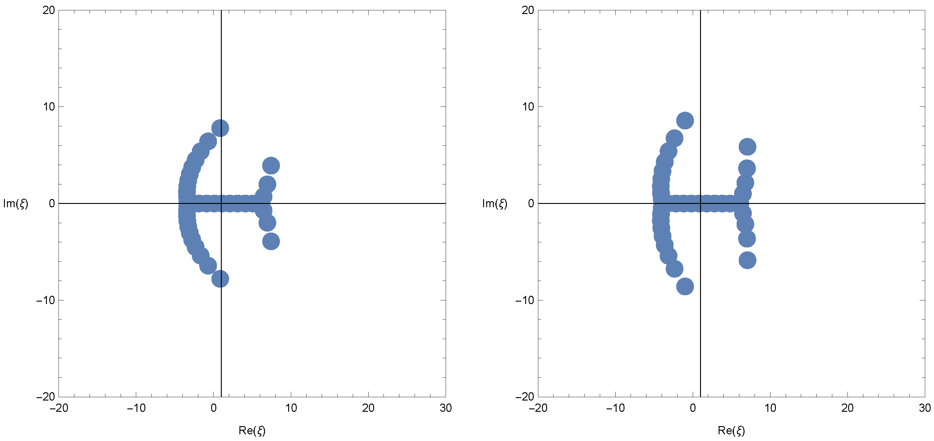
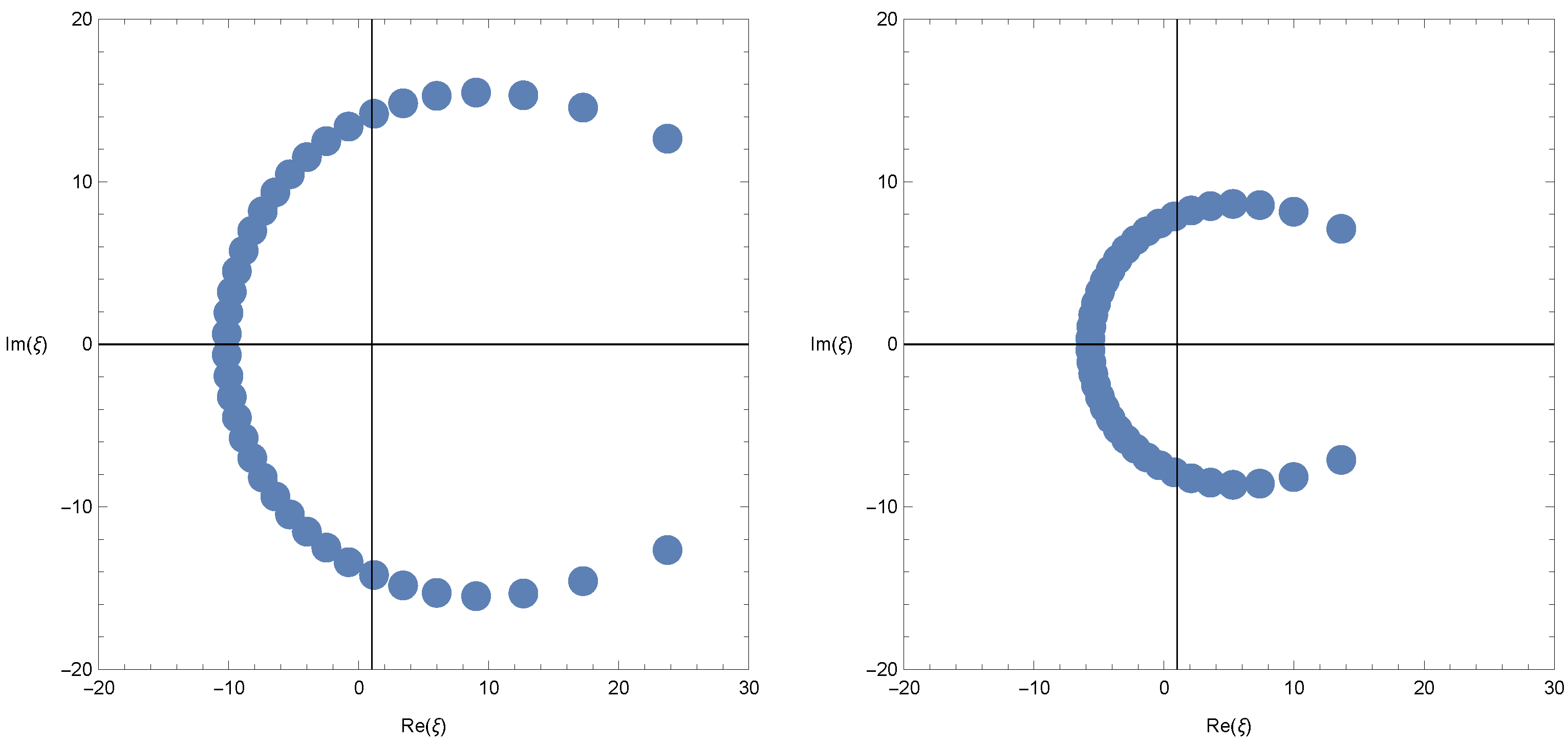
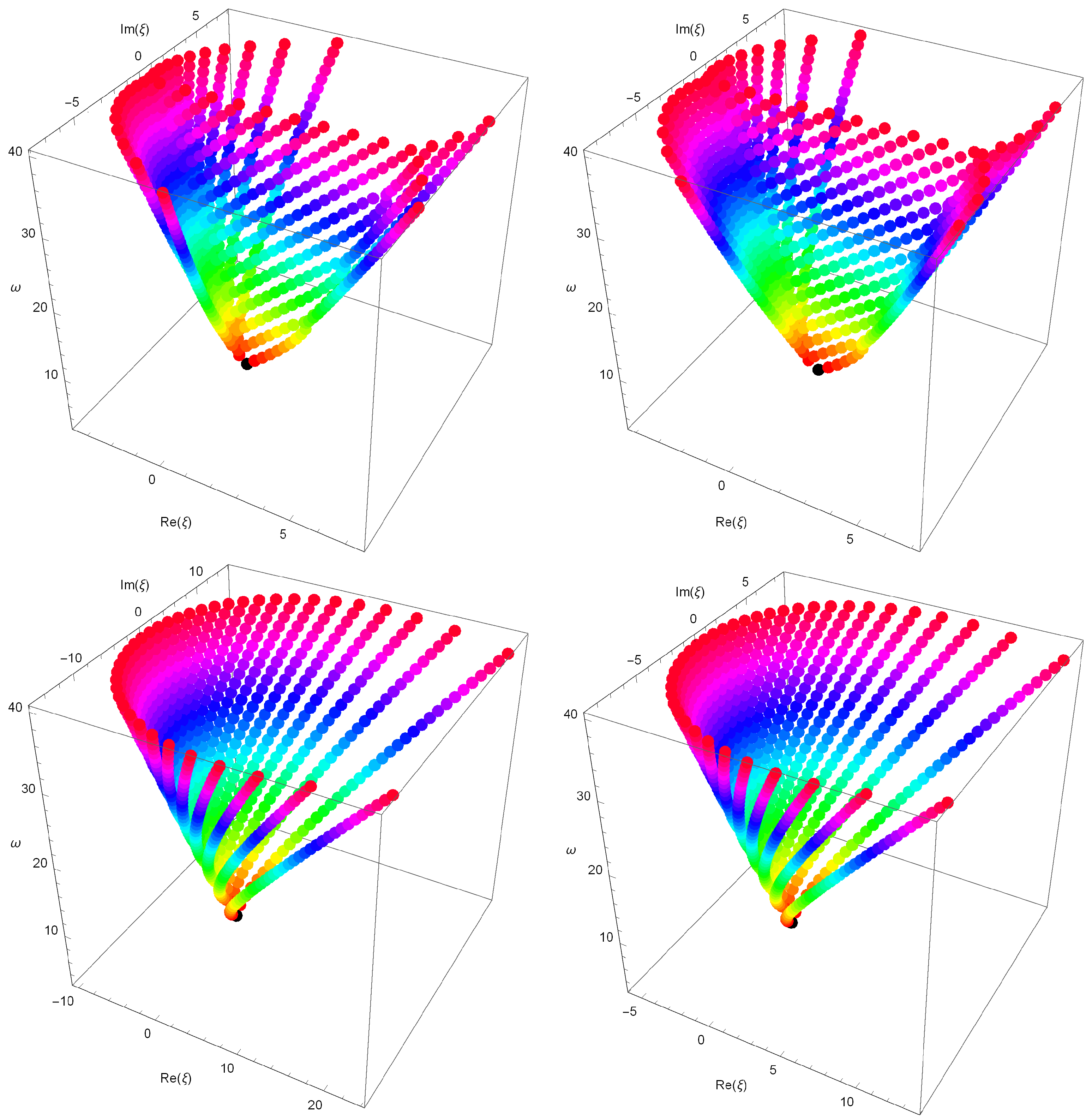
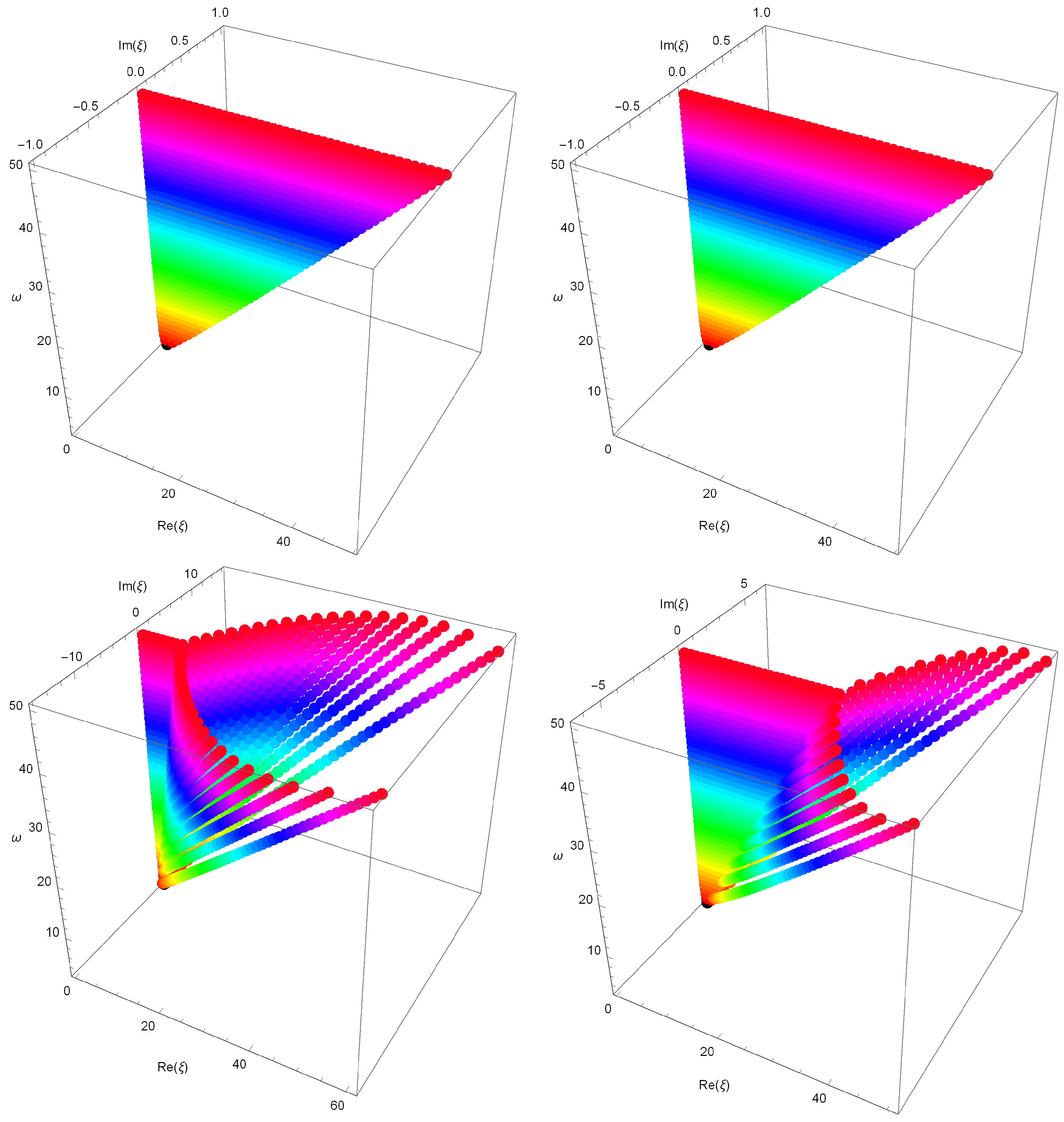
6. Computational Values and Graphical Representations of Frobenius–Euler–Genocchi Polynomials

In this section, certain zeros of the Frobenius–Euler–Genocchi polynomials ${\mathbb{A}}_{\omega }^{\left(2\right)}(\xi ;u)$ and beautifully graphical representations are shown. A few of them are

$$\begin{array}{}{\mathbb{A}}_0^{\left(2\right)}(\xi ;u)=0,\\ {\mathbb{A}}_1^{\left(2\right)}(\xi ;u)=0,\\ {\mathbb{A}}_2^{\left(2\right)}(\xi ;u)=2,\\ {\mathbb{A}}_3^{\left(2\right)}(\xi ;u)=\frac{6}{-1+u}-\frac{6\xi }{-1+u}+\frac{6u\xi }{-1+u},\\ {\mathbb{A}}_4^{\left(2\right)}(\xi ;u)=\frac{12}{{(-1+u)}^2}+\frac{12u}{{(-1+u)}^2}-\frac{24\xi }{{(-1+u)}^2}+\frac{24u\xi }{{(-1+u)}^2}+\frac{12{\xi }^2}{{(-1+u)}^2}\\ -\frac{24u{\xi }^2}{{(-1+u)}^2}+\frac{12u^2{\xi }^2}{{(-1+u)}^2},\\ {\mathbb{A}}_5^{\left(2\right)}(\xi ;u)=-\frac{20}{{(-1+u)}^4}-\frac{60u}{{(-1+u)}^4}+\frac{60u^2}{{(-1+u)}^4}+\frac{20u^3}{{(-1+u)}^4}-\frac{60\xi }{{(-1+u)}^3}\\ +\frac{60u^2\xi }{{(-1+u)}^3}-\frac{60{\xi }^2}{{(-1+u)}^2}+\frac{60u{\xi }^2}{{(-1+u)}^2}+\frac{20{\xi }^3}{1-u}-\frac{20u{\xi }^3}{1-u},\\ {\mathbb{A}}_6^{\left(2\right)}(\xi ;u)=\frac{720}{{(1-u)}^5}-\frac{1080}{{(1-u)}^4}+\frac{420}{{(1-u)}^3}-\frac{30}{{(1-u)}^2}-\frac{720u}{{(1-u)}^5}+\frac{1080u}{{(1-u)}^4}\\ -\frac{420u}{{(1-u)}^3}+\frac{30u}{{(1-u)}^2}-\frac{120\xi }{{(-1+u)}^4}-\frac{360u\xi }{{(-1+u)}^4}+\frac{360u^2\xi ]}{{(-1+u)}^4}+\frac{120u^3\xi }{{(-1+u)}^4}\\ -\frac{180{\xi }^2}{{(-1+u)}^3}+\frac{180u^2{\xi }^2}{{(-1+u)}^3}-\frac{120{\xi }^3}{{(-1+u)}^2}+\frac{120u{\xi }^3}{{(-1+u)}^2}+{\displaystyle \frac{(30{\xi }^4}{1-u}}-\frac{30u{\xi }^4}{1-u}.\end{array}$$

We investigate the beautiful zeros of the Frobenius–Euler–Genocchi polynomials ${\mathbb{A}}_{\omega }^{\left(2\right)}(\xi ;u)$ by using a computer. We plot the zeros of the Frobenius–Euler–Genocchi polynomials ${\mathbb{A}}_{\omega }^{\left(2\right)}(\xi ;u)=0$ for $\omega =40$ (Figure 1).

In Figure 1 (top left), we choose $r=2$ and $u=-7$. In Figure 1 (top right), we choose $r=2$ and $u=-3$. In Figure 1 (bottom-left), we choose $r=2$ and $u=3$. In Figure 1 (bottom-right), we choose $r=2$ and $u=7$.

Stacks of zeros of the Frobenius–Euler–Genocchi polynomials ${\mathbb{A}}_{\omega }^{\left(r\right)}(\xi ;u)=0$ for $3\le \omega \le 40$, forming a 3D structure, are presented (Figure 2).

In Figure 2 (top left), we choose $r=2$ and $u=-7$. In Figure 2 (top right), we choose $r=2$ and $u=-3$. In Figure 2 (bottom-left), we choose $r=2$ and $u=3$. In Figure 2 (bottom-right), we choose $r=2$ and $u=7$.

Next, we calculated an approximate solution satisfying the Frobenius–Euler–Genocchi polynomials ${\mathbb{A}}_{\omega }^{\left(2\right)}(\xi ;u)=0$ for $u=3$. The results are given in

Table 1. Approximate solutions of ${\mathbb{A}}_{\omega }^{\left(2\right)}(\xi ;u)=0$.

Degree $\mathit{\omega }$	$\mathit{\xi }$
3	−0.50000
4	−0.50000 − 0.86603i, −0.50000 + 0.86603 i
5	−1.0800, −0.2100 − 1.5819 i, −0.2100 + 1.5819 i
6	−1.1991 − 0.7701 i, −1.1991 + 0.7701 i,
	0.1991 − 2.2101 i, 0.1991 + 2.2101 i
7	−1.6268, −1.1130 − 1.4787i, −1.1130 + 1.4787 i,
	0.6764 − 2.7763 i, 0.6764 + 2.7763 i
8	−1.7906 − 0.7321 i, −1.7906 + 0.7321i, −0.9087 − 2.1385 i,
	−0.9087 + 2.1385 i, 1.1993 − 3.2957i, 1.1993 + 3.2957 i
9	−2.1611, −1.7990 − 1.4290 i, −1.7990 + 1.4290 i, −0.6261 − 2.7580 i,
	−0.6261 + 2.7580 i, 1.7556 − 3.7778 i, 1.7556 + 3.7778 i
10	−2.3477 − 0.7111 i, −2.3477 + 0.7111 i, −1.7030 − 2.0940 i,
	−1.7030 + 2.0940 i, −0.2870 − 3.3436 i, −0.2870 + 3.3436 i,
	2.3378 − 4.2296 i, 2.3378 + 4.2296 i
11	−2.6889, −2.4100 − 1.3992 i, −2.4100 + 1.3992 i,
	−1.5315 − 2.7306 i, −1.5315 + 2.7306 i, 0.0952 − 3.8998 i,
	0.0952 + 3.8998 i, 2.9407 − 4.6560 i, 2.9407 + 4.6560 i

.

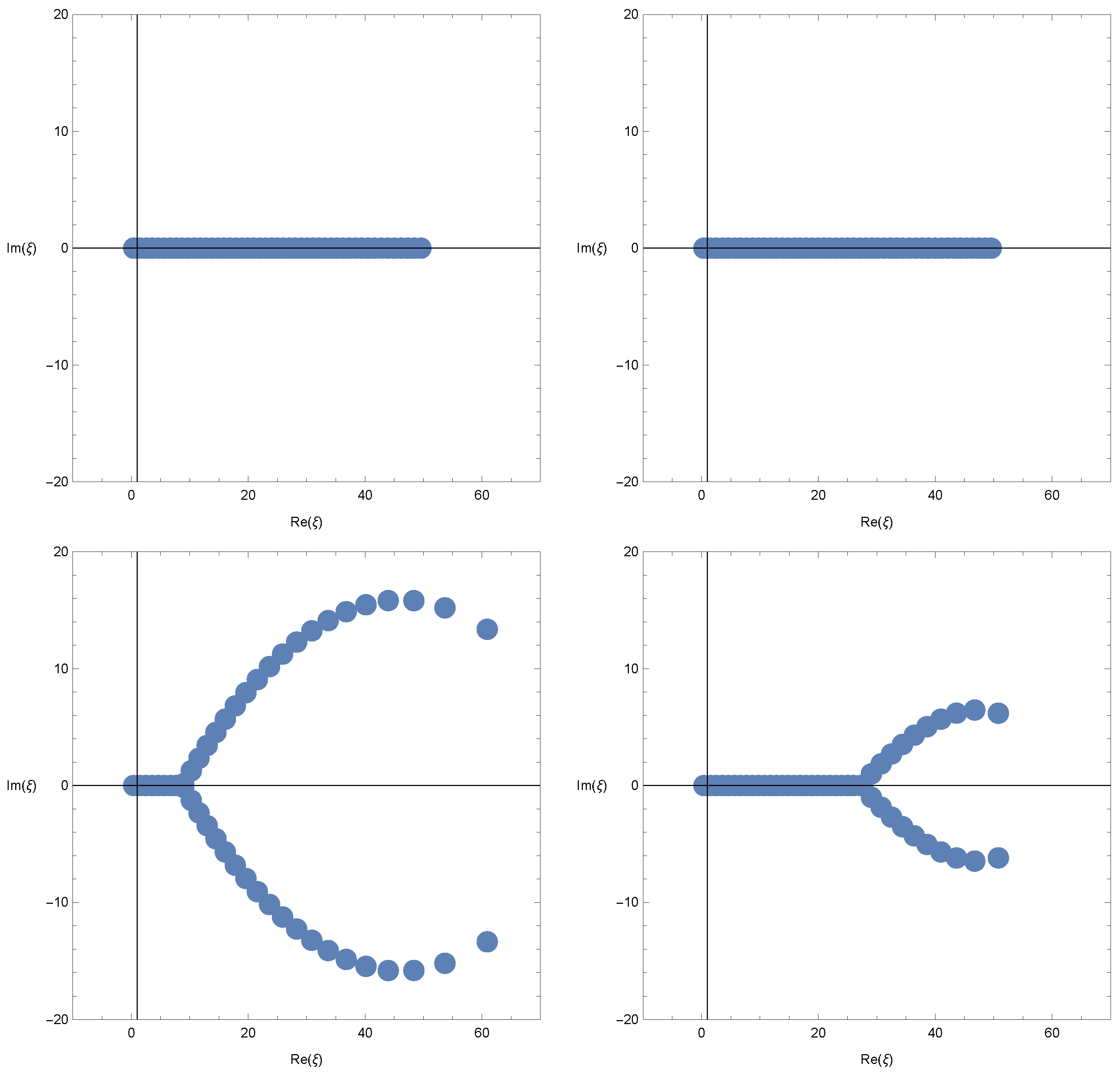
7. Computational Values and Graphical Representations of Changhee–Frobenius–Euler–Genocchi Polynomials

In this section, certain zeros of the Changhee–Frobenius–Euler–Genocchi ${}_C{\mathbb{G}}_{\omega }^{\left(r\right)}(\xi ;u)$ and beautifully graphical representations are shown. A few of them are

$$\begin{array}{}{}_C{\mathbb{G}}_1^{\left(2\right)}(\xi ;u)=0,\\ {}_C{\mathbb{G}}_2^{\left(2\right)}(\xi ;u)=2,\\ {}_C{\mathbb{G}}_3^{\left(2\right)}(\xi ;u)=\frac{12}{-1+u}-\frac{6u}{-1+u}-\frac{6\xi }{-1+u}+\frac{6u\xi }{-1+u},\\ {}_C{\mathbb{G}}_4^{\left(2\right)}(\xi ;u)=\frac{70}{{(-1+u)}^2}-\frac{68u}{{(-1+u)}^2}+\frac{22u^2}{{(-1+u)}^2}-\frac{60\xi }{{(-1+u)}^2}+\frac{96u\xi }{{(-1+u)}^2}-\frac{36u^2\xi }{{(-1+u)}^2}\\ +\frac{12{\xi }^2}{{(-1+u)}^2}-\frac{24u{\xi }^2}{{(-1+u)}^2}+\frac{12u^2{\xi }^2}{{(-1+u)}^2},\\ {}_C{\mathbb{G}}_5^{\left(2\right)}(\xi ;u)=\frac{450}{{(-1+u)}^3}-\frac{640u}{{(-1+u)}^3}+\frac{410u^2}{{(-1+u)}^3}-\frac{100u^3}{{(-1+u)}^3}-\frac{510\xi }{{(-1+u)}^3}+\frac{1110u\xi }{{(-1+u)}^3}\\ -\frac{810u^2\xi }{{(-1+u)}^3}+\frac{210u^3\xi }{{(-1+u)}^3}+\frac{180{\xi }^2}{{(-1+u)}^3}-\frac{480u{\xi }^2}{{(-1+u)}^3}+\frac{420u^2{\xi }^2}{{(-1+u)}^3}\\ -\frac{120u^3{\xi }^2}{{(-1+u)}^3}-\frac{20{\xi }^3}{{(-1+u)}^3}+\frac{60u{\xi }^3}{{(-1+u)}^3}-\frac{60u^2{\xi }^3}{{(-1+u)}^3}+\frac{20u^3{\xi }^3}{{(-1+u)}^3},\end{array}$$

$$\begin{array}{}{}_C{\mathbb{G}}_6^{\left(2\right)}(\xi ;u)=\frac{720}{{(1-u)}^5}+\frac{660}{{(1-u)}^3}+\frac{548}{1-u}+\frac{720}{{(-1+u)}^4}+\frac{600}{{(-1+u)}^2}-\frac{720u}{{(1-u)}^5}\\ -\frac{660u}{{(1-u)}^3}-\frac{548u}{1-u}-\frac{720u}{{(-1+u)}^4}-\frac{600u}{{(-1+u)}^2}-\frac{1080\xi }{{(1-u)}^3}-\frac{1350\xi }{1-u}\\ -\frac{720\xi }{{(-1+u)}^4}-\frac{1260\xi }{{(-1+u)}^2}+\frac{1080u\xi }{{(1-u)}^3}+\frac{350u\xi }{1-u}+\frac{720u\xi }{{(-1+u)}^4}+\frac{1260u\xi }{{(-1+u)}^2}\\ +\frac{360{\xi }^2}{{(1-u)}^3}+\frac{1020{\xi }^2}{1-u}+\frac{720{\xi }^2}{{(-1+u)}^2}-\frac{360u{\xi }^2}{{(1-u)}^3}-\frac{1020u{\xi }^2}{1-u}-\frac{720u{\xi }^2}{{(-1+u)}^2}\\ -\frac{300{\xi }^3}{1-u}-\frac{120{\xi }^3}{{(-1+u)}^2}+\frac{300u{\xi }^3}{1-u}+\frac{120u{\xi }^3}{{(-1+u)}^2}+\frac{30{\xi }^4}{1-u}-\frac{30u{\xi }^4}{1-u}.\end{array}$$

We plot the zeros of the Changhee–Frobenius–Euler–Genocchi ${}_C{\mathbb{G}}_{\omega }^{\left(r\right)}(\xi ;u)=0$ for $\omega =50$ (Figure 3).

In Figure 3 (top left), we choose $r=2$ and $u=-7$. In Figure 3 (top right), we choose $r=2$ and $u=-3$. In Figure 3 (bottom left), we choose $r=2$ and $u=3$. In Figure 3 (bottom right), we choose $r=2$ and $u=7$.

Stacks of zeros of the Changhee–Frobenius–Euler–Genocchi ${}_C{\mathbb{G}}_{\omega }^{\left(r\right)}(\xi ;u)=0$ for $3\le \omega \le 50$, forming a 3D structure, are presented (Figure 4).

In Figure 4 (top left), we choose $r=2$ and $u=-7$. In Figure 4 (top right), we choose $r=2$ and $u=-3$. In Figure 4 (bottom left), we choose $r=2$ and $u=3$. In Figure 4 (bottom right), we choose $r=2$ and $u=7$.

Next, we calculated an approximate solution satisfying the Changhee–Frobenius–Euler–Genocchi ${}_C{\mathbb{G}}_{\omega }^{\left(r\right)}(\xi ;u)=0$. The results are given in

Table 2. Approximate solutions of ${}_C{\mathbb{G}}_{\omega }^{\left(2\right)}(\xi ;-3)=0$.

Degree $\mathit{\omega }$	$\mathit{\xi }$
3	1.2500
4	0.97272, 2.5273
5	0.83715, 2.2045, 3.7084
6	0.75834, 2.0289, 3.3703, 4.8425
7	0.70700, 1.9225, 3.1696, 4.5035, 5.9475
8	0.67047, 1.8533, 3.0413, 4.2873, 5.6152, 7.0324
9	0.64266, 1.8052, 2.9562, 4.1418, 5.3905, 6.7113, 8.1024
10	0.62043, 1.7695, 2.8973, 4.0421, 5.2320, 6.4829, 7.7949, 9.1609
11	0.60202, 1.7414, 2.8545, 3.9723, 5.1194, 6.3151, 7.5666, 8.8684, 10.210
12	0.58638, 1.7185, 2.8218, 3.9220, 5.0389, 6.1915, 7.3925, 8.6427, 9.9333, 11.252

.

8. Conclusions

The theory of multidimensional or multi-index special functions is a very relevant field of investigation to simplify a wide range of operational relations. It has also been shown that Bell polynomials play a fundamental role in the extension of the classical special functions to the multidimensional case. In this article, we discuss a new class of generalized Frobenius–Euler–Genocchi polynomials and related special cases for the particular values of the parameters. We have used the generating Functions (15) and (26) to study their properties and related results. Using our result (15) and (26) to generalize the well-known class of Bernoulli, Euler, Genocchi, Changhee–Genocchi, and Bernoulli polynomials of the second kind. Moreover, for $r=0$, using the Faà di Bruno formula and some properties of the Bell polynomials of the second kind, we have presented an explicit formula for the Frobenius–Euler polynomials of order $\alpha$. We have given determinantal representations for the ratio of two differentiable functions. We have obtained a recursive relation for the Frobenius–Euler polynomials of order $\alpha$. Finally, we have checked the roots and graphical representations of these types of polynomials by making use of Mathematica software. Based on this article, readers can apply the method we presented in the article to many polynomials.

References

1. Alatawi, M.S.; Khan, W.A. New type of degenerate Changhee-Genocchi polynomials. Axioms 2022, 11, 355. [Google Scholar] [CrossRef]
2. Luo, Q.-M. On the Apostol Bernoulli polynomials. Cent. Eur. J. Math. 2004, 2, 509–515. [Google Scholar] [CrossRef]
3. Belbachir, H.; Hadj-Brahim, S. Some explicit formulas of Euler-Genocchi polynomials. Integers 2019, 19, 1–14. [Google Scholar]
4. Carlitz, L. Eulerian numbers and polynomials. Math. Mag. 1959, 32, 247–260. [Google Scholar] [CrossRef]
5. Choi, J.; Kim, D.S.; Kim, T.; Kim, Y.H. A note on some identities of Frobenius-Euler numbers and polynomials. Int. J. Math. Math. Sci. 2012, 2012, 861797. [Google Scholar] [CrossRef] [Green Version]
6. Goubi, M. On a generalized family of Euler-Genocchi polynomials. Integers 2021, 21, 1–13. [Google Scholar]
7. Iqbal, A.; Khan, W.A.; Nadeem, M. New Type of Degenerate Changhee-Genocchi Polynomials of the Second Kind. In Soft Computing: Theories and Applications; Kumar, R., Verma, A.K., Sharma, T.K., Verma, O.P., Sharma, S., Eds.; Lecture Notes in Networks and Systems; Springer: Berlin/Heidelberg, Germany, 2023; Volume 627. [Google Scholar]
8. Iqbal, A.; Khan, W.A. A New Family of Generalized Euler-Genocchi Polynomials Associated with Hermite Polynomials. In Soft Computing: Theories and Applications; Kumar, R., Verma, A.K., Sharma, T.K., Verma, O.P., Sharma, S., Eds.; Lecture Notes in Networks and Systems; Springer: Berlin/Heidelberg, Germany, 2023; Volume 627. [Google Scholar]
9. Kim, T.; Kim, D.S.; Kim, H.K. On generalized degenerate Euler-Genocchi polynomials. Appl. Math. Sci. Eng. 2023, 31, 1. [Google Scholar] [CrossRef]
10. Nadeem, M.; Khan, W.A. Symmetric Identities For Degenerate q-Poly-Genocchi Numbers And Polynomials. South East Asian J. Math. Math. Sci. 2023, 19, 17–28. [Google Scholar] [CrossRef]
11. Srivastava, H.M.; Pinter, A. Remarks on some relationships between the Bernoulli and Euler polynomials. Appl. Math. Lett. 2004, 17, 375–380. [Google Scholar] [CrossRef] [Green Version]
12. Kim, D.S.; Kim, T.; Seo, J. A note on Changhee polynomials and numbers. Adv. Stud. Theor. Phys. 2013, 7, 993–1003. [Google Scholar] [CrossRef]
13. Kwon, H.-I.; Kim, T.; Park, J.W. A note on degenerate Changhee-Genocchi polynomials and numbers. Glob. J. Pure Appl. Math. 2016, 12, 4057–4064. [Google Scholar]
14. Kim, B.-M.; Jeong, J.; Rim, S.-H. Some explicit identities on Changhee-Genocchi polynomials and numbers. Adv. Differ. Equ. 2016, 202, 1–12. [Google Scholar] [CrossRef] [Green Version]
15. Yasar, B.Y.; Ozarslan, M.A. Frobenius-Euler and Frobenius-Genocchi polynomials and their differential equations. New Trend Math. Sci. 2015, 3, 172–180. [Google Scholar]
16. Kim, D.S.; Kim, T. Some new identities of Frobenius-Euler numbers and polynomials. J. Inequal. Appl. 2012, 2012, 307. [Google Scholar] [CrossRef] [Green Version]
17. Kim, D.S.; Kim, T. Higher-order Frobenius-Euler and poly-Bernoulli mixed-type polynomials. Adv. Differ. Equ. 2013, 2013, 251. [Google Scholar] [CrossRef] [Green Version]
18. Srivastava, H.M.; Boutiche, M.A.; Rahmani, M. Some explicit formulas for the Frobenius- Euler polynomials of higher order. Appl. Math. Inf. Sci. 2017, 11, 621–626. [Google Scholar] [CrossRef]
19. Kurt, B.; Simsek, Y. On the generalized Apostol-type Frobenius-Euler polynomials. Adv. Differ. Equ. 2013, 2013, 1. [Google Scholar] [CrossRef] [Green Version]
20. Cakić, N.P.; Milovanović, G. On generalized Stirling number and polynomials. Math. Balk. 2004, 18, 241–248. [Google Scholar]
21. Jamei, M.J.; Milovanović, G.; Dagli, M.C. A generalization of the array type polynomials. Math. Moravica 2022, 26, 37–46. [Google Scholar] [CrossRef]
22. Luo, Q.M.; Srivastava, H.M. Some generalization of the Apostol-Genocchi polynomials and Stirling numbers of the second kind. Appl. Math. Comput. 2011, 217, 5702–5728. [Google Scholar] [CrossRef]
23. Belbachir, H.; Hadj-Brahim, S.; Rachidi, M. On another approach for a family of Appell polynomials. Filomat 2018, 12, 4155–4164. [Google Scholar] [CrossRef]
24. Borisov, B.S. The p-binomial transform Cauchy numbers and figurate numbers. Proc. Jangjeon Math. Soc. 2016, 19, 631–644. [Google Scholar]
25. Wang, Y.; Dagli, M.C.; Liu, X.-M.; Qi, F. Explicit, determinantal, and recurrent formulas of generalized Eulerian polynomials. Axioms 2021, 10, 37. [Google Scholar] [CrossRef]
26. Qi, F.; Guo, B.-N. Explicit formulas for special values of the Bell polynomials of the second kind and for the Euler numbers and polynomials. Mediterr. J. Math. 2017, 14, 140. [Google Scholar] [CrossRef]
27. Kızılateş, C. Explicit, determinantal, recursive formulas, and generating functions of generalized Humbert-Hermite polynomials via generalized Fibonacci Polynomials. Math. Methods Appl Sci. 2023, 46, 9205–9216. [Google Scholar] [CrossRef]
28. Dagli, M.C. Explicit, determinantal, recursive formulas and relations of the Peters polynomials and numbers. Math. Methods Appl. Sci. 2022, 45, 2582–2591. [Google Scholar] [CrossRef]
29. Qi, F.; Dağlı, M.C.; Lim, D. Several explicit formulas for (degenerate) Narumi and Cauchy polynomials and numbers. Open Math. 2021, 19, 833–849. [Google Scholar] [CrossRef]
30. Qi, F.; Zheng, M.-M. Explicit expressions for a family of the Bell polynomials and applications. Appl. Math. Comput. 2015, 258, 597–607. [Google Scholar] [CrossRef] [Green Version]
31. Qi, F.; Niu, D.-W.; Lim, D.; Yao, Y.-H. Special values of the Bell polynomials of the second kind for some sequences and functions. J. Math. Anal. Appl. 2020, 491, 124382. [Google Scholar] [CrossRef]
32. Comtet, L. Advanced Combinatorics: The Art of Finite and Infinite Expansions; Springer Science & Business Media: Berlin/Heidelberg, Germany, 1974. [Google Scholar]
33. Bourbaki, N. Functions of a Real Variable, Elementary Theory, Translated from the 1976 French original by Philip Spain. In Elements of Mathematics; Springer: Berlin/Heidelberg, Germany, 2004. [Google Scholar]
Figure 1. Zeros   of   A ω ( r ) ( ξ ; u ) = 0 .
Symmetry 15 01358 g001aSymmetry 15 01358 g001b
Figure 2. Zeros   of   A ω ( r ) ( ξ ; u ) = 0 .
Symmetry 15 01358 g002
Figure 3. Zeros   of   C G ω ( r ) ( ξ ; u ) = 0 .
Symmetry 15 01358 g003
Figure 4. Zeros   of   H n , q ( α , c ) ( x , y ; u ; λ ) .
Symmetry 15 01358 g004