Wavelet Multiscale Granger Causality Analysis Based on State Space Models

Abstract

Granger causality (GC) is a popular method in causal linkage recovery and has been applied to various fields, such as economics and neuroscience. While the conventional Granger causality model is capable of identifying symmetrical causal relationships among variables, it is the asymmetric Granger causality that provides a more comprehensive perspective of the short- and long-term interactions between variables, which is of greater value for empirical study. Traditional vector autoregressive models lack the ability to explore multiscale information flow and are affected by the moving average component. Therefore, by combining the wavelet-based approach and state space model, we propose a new Granger causality analysis method to overcome the inherent limitation of vector autoregressive models and extend to multiscale causality exploration. Two simulations were conducted to compare the proposed approach to an existing wavelet-based method, and five evaluation indicators were utilized. The results indicate that the proposed method efficiently identifies the accurate asymmetric causalities at varying scales, while improving accuracy and reducing bias as compared to the current wavelet-based method. In conclusion, the combination of the wavelet approach and state space method enhances the multiscale causality detecting capability and can potentially contribute to multiscale Granger causality research.

1. Introduction

Granger causality, which was proposed and refined by Norbert Wiener and Clive Granger, is primarily used to establish the presence of causal linkages across variables in econometric research [1].

In 1956, Norbert Wiener [2] first suggested that Y could be called the cause of X if adding the information of Y would improve the prediction of X. However, it was not until 1969 that Clive Granger provided a concrete implementation of a linear autoregressive model based on the stochastic process [3].

In the simplest bivariate case, Granger causality is calculated by first dividing the variables X and Y into two sets: one set contains all the variables and the other only contains the target variable X, which are used to constructed two separate vector autoregressive (VAR) models—the full VAR models and the restricted VAR models. These give the residual covariance matrices of the two models, and the Granger causality from Y to X can be defined as the likelihood ratio of residual covariance between the restricted and full models.

Since Granger causality is related to the flow of information across variables, it has been used in a growing number of studies in various fields, including the inference of information flow in the human brain as well as the analysis of economic and engineering data [4,5,6,7,8]. With the growing number of potential applications, Granger causality analysis is increasingly being employed to investigate multivariate and multiscale data scenarios. Moreover, recent research has explored the potential to extend Granger causality analysis to the compression domain, highlighting the versatility and adaptability of this technique to various applications and fields [9].

However, the traditional VAR models only consider the bivariate case, which may be affected by confounding factors or joint distributions in the multivariate case. Furthermore, traditional VAR models are unable to take into account the dynamic complexity of individual processes at various time scales and therefore need to be modified to apply to multiscale data, or we can consider investigating other models that are more suitable for multivariate or multiscale analysis.

Geweke [10] originally introduced the concept of symmetric Granger causality, which refers to a dual causality relationship between two variables, whereby X Granger causes Y, and Y Granger causes X simultaneously, and generalized Granger causality to a multivariate approach that has been developed and well proven throughout time [11].

Although there are several restrictions, using VAR models for Granger causality analysis typically necessitates that the data adhere to the smoothness and linearity criteria. If there is a co-dependent third variable for both variables, it may lead to a spurious causal relationship, which can be eliminated by considering co-dependencies. When dealing with exogenous or latent variables, it may be challenging to entirely eliminate their confounding effects. Nonetheless, in such situations, the application of conditional Granger causality can help reduce their impact on the analysis to a certain extent [12].

A Matlab toolbox named Granger causal connectivity analysis (GCCA) developed by Seth A. K. et al. [13] in 2010 can be used to conduct Granger causal linkage analysis on various neuroscience data, including functional magnetic resonance imaging (fMRI). The updated multivariate Granger causality (MVGC) toolbox applied to multivariate variables was proposed in 2014. It contains computations for conditional and unconditional, time and frequency domains, and pairwise Granger causality based on the VAR model [14], helping to discover symmetric and asymmetric Granger causality.

Even though the VAR model is straightforward and simple to estimate, it has a significant limitation, in that moving average components can lead to an infinite number of model orders or require a larger number of model orders to model a finite number of small samples. This not only reduces the statistical effectiveness but also enhances biases, weakening the ability to obtain accurate estimates of Granger causality. Moving average components are common in time series modeling, whether they are inherent to the time series itself, or generated during data sampling and processing.

Numerous research studies have sought to minimize estimation bias when applying Granger causality analysis. One of the proposed solutions involves utilizing a combination of lasso regression and genetic algorithm, facilitated by initialization, selection, feature cross over, and mutation, to overcome coefficient overfitting [15]. Similarly, a new unified Granger causality method has been proposed, addressing the inconsistency between model order selection criteria and hypothesis testing procedures [16]. This method utilizes the minimum description length principle to reconcile the two stages, offering a promising approach for future multiscale research.

The state space model has been applied to overcome moving average components and demonstrated that it can achieve better statistical power and less bias than the traditional AR model as well as a strong Granger causality maintained with noise and downsampling [17,18]. These are due to the fact that the state space model has the equivalence to the auto regression moving average (ARMA) model and is independent of noise and downsampling [19]. Additionally, the state space model was integrated with recurrent neural networks by the researchers in order to increase prediction accuracy by accounting for background information that might have an impact on the target time series [20].

Complex system time series with multiscale features are very common in practical applications, such as heartbeat signals, rainfall time series, and electroencephalogram data [21,22,23]. Time series with multiscale characteristics usually fluctuate at different time scales, implying that system transformations have a multi-level time scale structure and time domain localization characteristics. This is the aspect that traditional time domain Granger causality analysis cannot investigate. It is crucial to consider approaches to overcome the limitations of the VAR model, better accommodate the multiscale features of the data, and improve the precision of Granger causality analysis.

Costa et al. [24] presented a multiscale entropy approach and used it to analyze the multiscale properties of the cardiovascular signals data. Faes et al. [25] proposed a multivariate stochastic process analysis framework based on the state space model. This framework explored a weighted average rescaling operation, which equals to the effects of averaging and downsampling. The authors successfully applied this method to explore multiscale Granger relationships using carbon dioxide (CO${}_2$) and global temperature data.

Reducing CO${}_2$ emissions is a crucial aspect of sustainable development. Recent studies have analyzed the factors that influence CO${}_2$ emissions from various perspectives such as technology and innovation, financial development, and human development. Policy advice is provided based on these analyses.

A panel causality analysis using the cross-sectional autoregressive distributed lag (CS-ARDL) method was conducted to investigate the factors affecting CO${}_2$ emissions in a panel of BRICS (i.e., Brazil, Russia, India, China, and South Africa) countries [26]. Similarly, the impact of greenhouse gas emissions on the Group of Seven economy was studied from the viewpoint of environment-related information and communication technologies innovations [27]. Adebayo et al. adopt the Fourier quantile causality test to examine the causal impact of environmental quality in China [28]. The study explores the causal relationships between CO${}_2$ emissions, ecological footprint, and load capacity factor.

However, as society develops, CO${}_2$ emissions display diverse patterns over time. Therefore, a multiscale analysis can better assist researchers in identifying causal relationships at various time scales.

The multiscale analysis is generally used to evaluate the intrinsic structure of a single time series and the multiscale representation of the interaction of information from two time series. It assesses the multiscale dynamic nature of a sequence by resampling the original time series of a complex process at different time scales, thus revealing the structure at multiple time scales and better reflecting information about the dynamics of the complex system [29].

In order to better analyze multiscale data, Lungarella M et al. proposed multiscale transfer entropy based on wavelet transform [30]. This method projects the time series into wavelet space to obtain a new set of variables from which causal linkages can be extracted at many scales.

The wavelet transform is a signal processing technique that represents instantaneous or non-stationary signals in terms of time and scale distributions, and it has good localization capabilities for localizing time series [31].

Stramaglia et al. introduced a wavelet-based multiscale Granger analysis technique that overcomes the computational complexity associated with filtering and downsampling at multiple scales [32]. The method employs the $\acute{a}$ trous wavelets that maintain translation invariance in the processing of time series, with decomposition coefficients at every level equating to the original time series length. The wavelet-transformed data are then utilized as a substitute for the driving variable data for Granger causality analysis. It is worth noting, however, that this approach depends on the VAR model’s inherent weaknesses previously mentioned, which may potentially increase the likelihood of producing inaccurate results.

Although multiscale Granger causality has been subjected to extensive research, the majority of these studies have employed the VAR model without addressing its limitations.

To improve the limitations mentioned in this section, the state space model with the advantage of downsamplng independence and the equality to ARMA model is considered in this paper, and a multiscale wavelet analysis framework based on the state space model is proposed, which can improve the accuracy and robustness of Granger causality compared to the VAR model.

The paper is structured into the following sections. Section 2 provides definitions of multiscale Granger causality and state space models and introduces the proposed approach in detail. Section 3 outlines the evaluation indicators adopted in this research and presents a comparative experiment between the methods of this paper and the wavelet-based method. The experimental results are then illustrated and discussed. Lastly, Section 4 concludes the study and offers suggestions for future work.

2. Materials and Methods

2.1. Granger Causality

Start with n smooth complex processes $Y_n={[y_{1,n},\dots ,y_{M,n}]}^T$, which are composed of M zero-mean scalar processes, respectively. Suppose $y_j$ is the target variable and $y_i$ is the driver variable, then the remaining $M-2$ processes of $Y_n$ make up $Y_k$, where k denotes the difference set of $\{1,2,\dots ,M\}$ and $\{i,j\}$. Let $Y_n^{-}$ denotes the past information of $Y_n$, $y_n^{-}$ denotes the past information of $y_n$. Then, the Granger causality from $y_i$ to $y_j$ means the extent of predicted improvement that based on the use of $y_{j,n}^{-}$ and $Y_{k,n}^{-}$ to predict $y_{j,n}$, the addition of $y_{i,n}^{-}$ makes.

Use all past processes to predict the present of target variable, which is named full regression. The prediction error for this method can be determined using the following equation:

$${\epsilon }_n=y_{j,n}-\mathbb{E}\left[y_{j,n}\right|Y_n^{-}]$$

(1)

where $\mathbb{E}$ is the expectation operator.

The prediction error of the restricted regression is obtained by using the past of all variables, except the driving variable to predict the present of the target variable as follows:

$${\epsilon }_n^R=y_{j,n}-\mathbb{E}\left[y_{j,n}\right|y_{j,n}^{-},Y_k^{-}]$$

(2)

where the superscript R represents reduced regression.

By calculating the log-likelihood values of the two regression prediction errors which are $\lambda =\mathbb{E}\left[{\epsilon }_n{\epsilon }_n^T\right]$ and ${\lambda }^R=\mathbb{E}\left[{\epsilon }_n^R{\left({\epsilon }_n^R\right)}^T\right]$, where the superscript T represents the transpose. The Granger causality values from $y_i$ to $y_j$ can be obtained as follows:

$$F_{i\to j}=ln\frac{{\lambda }^R}{\lambda }$$

2.2. State Space Model

Consider a general constant state space (SS) model,

$$\begin{array}{cc}\hfill X_{t+1}& =A{X}_t+W_t\hfill \\ \hfill Y_t& =C{X}_t+V_t\hfill \end{array}$$

(3)

where $W_t$ and $V_t$ are noisy variables with semi-positive definite covariance, which means $var\left(\begin{array}{c}{W}_t\\ V_t\end{array}\right)=\left(\begin{array}{cc}Q& S\\ S^T& R\end{array}\right)$. The parameters for model $\left(3\right)$ is $(A,C,Q,R,S)$.

After projecting the state variable onto the space tensed by the past of the observed variable, that is $Z_t=\mathbb{E}\left\{X_t|Y_{t-1}^{-}\right\}$, where $Y_{t-1}^{-}={\left[Y_{t-1}^T,Y_{t-2}^T\dots \right]}^T$ is an infinite column vector. $Z_t$ can also be considered the new state variable as well as the residuals of a linear regression on the variable $y_t$, using infinite past.

In this way, the innovations of state space model (ISS) for $Z_t$ which is equal to SS model can be described as follows:

$$\begin{array}{cc}\hfill Z_{t+1}& =A{Z}_t+K{E}_t,\hfill \\ \hfill Y_t& =C{Z}_t+E_t\hfill \end{array}$$

(4)

where the innovation is defined as $E_t\equiv Y_t-\mathbb{E}\left\{Y_t|Y_{t-1}^{-}\right\}$, with covariance matrix $\Sigma \equiv \mathbb{E}\left\{E_t{E}_t^T\right\}$. The parameters for model (4) are $(A,C,K,\Sigma )$.

According to the ISS model, the error of the full regression can be obtained as ${\lambda }_{full}=\Sigma (j,j)$. In order to obtain the error of the restricted regression, we consider the state space model (4) with the submodel, removing the driving variable. In this regard, the first equation retains the same form as in (4), while the second equation is formulated as follows:

$$\begin{array}{cc}\hfill Z_{t+1}& =A{Z}_t+K{\epsilon }_t,\hfill \\ \hfill Y_t^{\left(jk\right)}& =C^{\left(jk\right)}{Z}_t+{\epsilon }_t^{\left(jk\right)}\hfill \end{array}$$

(5)

where the superscript $\left(jk\right)$ denotes the selection of the $j,k$ rows in the matrix. At this point, the parameters of the state space model (5) are $(A,C^{\left(jk\right)},K\Sigma K^T,\Sigma (jk,jk),K\Sigma (:,jk))$. It is notable that the ISS model and the SS model are mutually interchangeable as reported by Barnett and Takahashi in 2015 [17]. Specifically, the parameters of the SS model can be transformed into corresponding parameters of the ISS model by resolving the DARE equation. By implementing this transformation, the error ${\lambda }_{restricted}={\Sigma }^R(j,j)$ of the constrained model can be deduced.

Finally, the Granger causality can be calculated as follows:

$$F_{i\to j}=ln\frac{{\Sigma }^R(j,j)}{\Sigma (j,j)}$$

2.3. Wavelet Transform

The approach of the wavelet transform, which is grounded on the short-time Fourier transform, provides a possibility for local analysis of time–frequency through examination of the fluctuation of each moment or spatial position across multiple time scales. Distinct from the Fourier transform, the wavelet transform exhibits tight support and, therefore, proves to be advantageous for investigating well-defined signals confined within a specific temporal window.

Let $\psi \left(t\right)$ be the mother wavelet, and a stretching translation yields the subwavelet ${\psi }_{a,b}\left(t\right)=\frac{1}{\sqrt{a}}\psi \left(\frac{t-b}{a}\right)$, where $a\ne 0$ is called the scale factor for stretching, and $\frac{1}{\sqrt{a}}$ ensures that ${\psi }_{a,b}\left(t\right)$ has a norm value of 1; b is called the translation factor and is used to translate. Then the discrete wavelet transform of the signal $f\left(t\right)$ is defined as the function about a and b, which obtains the projection of the original signal $f\left(t\right)$ onto the mother wavelet. The * in the following equation means complex conjugation:

$$W_{\psi }f(a,b)=\sum _{t}f\left(t\right){\psi }_{a,b}^{\ast }\left(t\right)$$

Several mother wavelets are frequently utilized in signal analysis, such as Haar wavelets, Mexican cap wavelets, and Morlet wavelets. However, not all wavelets are appropriate for this purpose. For instance, while Mallat wavelets utilize orthogonal bases, they lack translation invariance. As such, to acquire a translation-invariant wavelet decomposition, the discrete wavelet transform of the $\acute{a}$ trous algorithm is implemented for signal decomposition.

The $\acute{a}$ trous algorithm separates the high-frequency and low-frequency information in the signal $f\left(t\right)$ by repeatedly using low-pass filtering $h\left(n\right)$. In this paper, $h=\frac{1}{16}[1,4,6,4,1]$ is chosen as the low-pass filter. The high-frequency information corresponds to the coefficient terms of the wavelet transform and the low-frequency information corresponds to the approximation terms of the wavelet coefficients. The approximation of the signal at each scale is first obtained:

$$a_s\left(t\right)=\sum _{n}h\left(n\right)a_{s-1}(t+2^{s-1}n)(s=1,\dots ,N)$$

where $a_0\left(t\right)$ is the original discrete signal $f\left(t\right)$, $n=1,2,\dots ,5$, s is the scale index, and N is the maximum number of scales. Then the wavelet coefficients are defined as $c_s\left(t\right)=a_{s-1}\left(t\right)-a_s\left(t\right)$. The reconstruction of the signal is completed by adding the last smoothed signal $a_N\left(t\right)$ and the wavelet coefficients at all scales as follows:

$$f\left(t\right)=a_N\left(t\right)+\sum _{s=1}^N{c}_s\left(t\right)$$

It is worth noting that the $\acute{a}$ trous algorithm has the same length at each scale as the original signal, which allows the signal to be decomposed without bias, as well as better detection of detailed signals.

2.4. The Analysis Framework Proposed in This Paper

Building on the theories explained earlier, this paper introduces a novel method called Granger causality with wavelet transform and state space model (GTSS), which considers replacing the driving variable $y_i$ with the wavelet coefficients at the corresponding scale and using state space model for Granger causality analysis. Since the restricted regression does not use the data of the driving variable $y_i$, the error of the restricted regression is not affected by the wavelet transform and remains as shown in Equation (2). Meanwhile, the prediction error of the full regression is ${\epsilon }_s=y_j-\mathbb{E}\left[y_j\right|y_j^{-},Y_k^{-},c_s^{-}]$, then we can gain the variance by ${\Sigma }_s^R(j,j)=\mathbb{E}\left[{\epsilon }_s{\epsilon }_s^T\right]$.

Therefore, under the scale s, the Granger causality values from $y_i$ to $y_j$ can be obtained as follows:

$$F_{i\to j}^s=ln\frac{{\Sigma }_s^R(j,j)}{\Sigma (j,j)}$$

The proposed analytical framework of GTSS involves the following steps:

Step 1: Employ the $\acute{a}$ trous wavelets as the mother wavelet to perform wavelet decomposition on the original time series, and obtain the wavelet coefficients $C_n=[c_{1,n},\dots ,c_{N,n}]$ at each scale.

Step 2: Replace the data of driving variable $y_i$ with the wavelet coefficients $c_s$ for scale s, resulting in $Y^s={[y_{1,n},\dots ,y_{i-1,n},c_{s,i},y_{i+1,n},\dots ,y_{M,n}]}^T$.

Step 3: Estimate the model parameters using the modified $Y^s$ and calculate the Granger causality values at scale s.

Step 4: Repeat Step 2 to 3 by varying the scale value s.

Step 5: Save the Granger causality values across multiple scales.

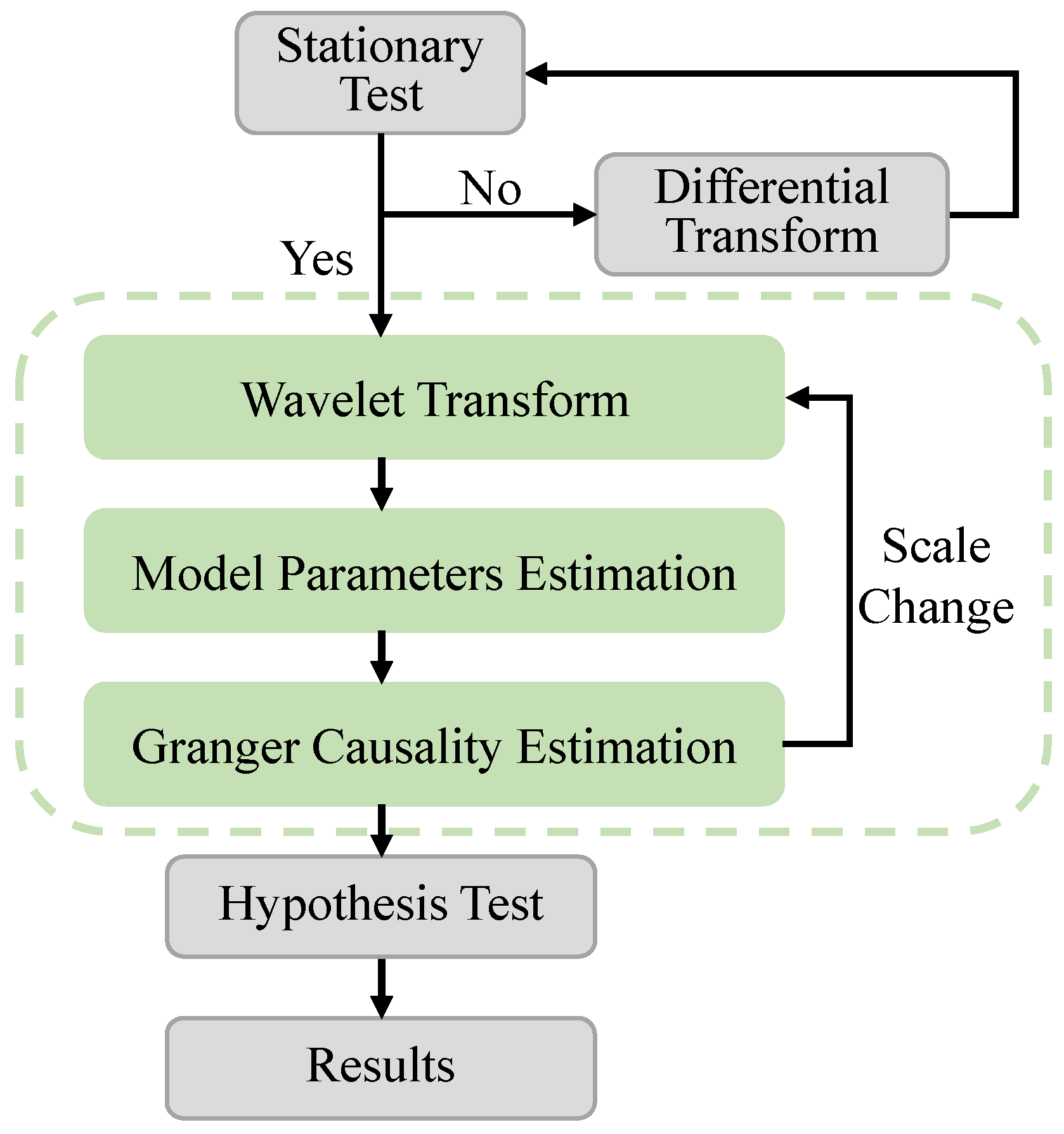
The flow of empirical analysis is presented in Figure 1 which adopts a multi-step methodology.

The process begins with conducting the augmented Dickey–Fuller (ADF) stationary test. If the data are observed to be stationary, Granger causality analysis follows. Alternatively, if the data are non-stationary, differential transform is performed until stationarity is obtained before proceeding with the GTSS method. The GTSS method involves wavelet transform, including wavelet decomposition and wavelet coefficient replacement, followed by Granger causality estimation at each scale s. The process iterates by changing the scale value s and repeating wavelet transform and causality estimation. Upon obtaining the hypothesis test results through the GTSS method, evaluation indicators, such as the reject rate and mean square error, are calculated to confirm the presence of a causal relationship.

3. Simulation Study and Results

This section presents experiments on Granger causality with the wavelet transform method (GT) proposed by Stramaglia S. et al. [32] and the GTSS method proposed in this paper, analyzing the results for the bivariate and multivariate cases, respectively, and comparing the advantages and disadvantages of the two methods.

3.1. Evaluation Indicator

The following experiments incorporate several evaluation indices that assist in the analysis. The calculation of each is explained below.

First, the coefficient bias [8] between the estimated and defined values of the VAR models is calculated to investigate the validity of the model estimation method in this paper. The coefficient bias (CB) is defined as follows:

$$\mathrm{CB}=\frac{{∥A-AT∥}_1}{{∥A∥}_1}$$

where ${∥•∥}_1$ is the L1 norm, A is the estimated value of the model coefficient matrix, and $AT$ is a pre-defined model coefficient matrix.

However, due to the absence of prior knowledge of the actual causal flow in reality, it is difficult to determine the accuracy of the utilized model, which is typically evaluated by comparing to the real causality. To address this challenge, we developed the reject rate and overall reject rate as evaluation metrics for assessing causal outcomes.

The reject rate (RR), which is calculated according to the significance tests’ results, is defined as follows:

$$\mathrm{RR}=\frac{NRS}{TNS}$$

where $NRS$ represents the number of rejections for significance tests, and $TNS$ represents the total number for significance tests.

This evaluation index measures the innate detection capability of the algorithm. A low rejection rate in instances of actual causality suggests that the algorithm is proficient in generating accurate estimates without resorting to hypothesis testing, thereby reducing reliance on such methods. Conversely, a high rejection rate in situations where no actual causality exists demonstrates that the accuracy of the estimate can be improved through the application of hypothesis testing techniques.

To better see the overall effect, in this paper, the reject rates in both cases are combined into one indicator named overall reject rate (ORR) as follows:

$$\mathrm{ORR}=RRE+1-RRN$$

where $RRE$ is the reject rate where Granger causality exists, and $RRN$ represents the reject rate for when it does not exist.

The mean square error (MSE) from i to j and accuracy are used in the simulation study and calculated as follows:

$${\mathrm{MSE}}_{i\to j}=\frac{1}{ntrial}{\Sigma }_{n=1}^{ntrial}{(G{C}_n-G{C}_t)}^2$$

where $ntrial$ is the number of trials, $G{C}_n$ is the estimated Granger causality value from i to j in the $n\mathrm{th}$ trial, and $G{C}_t$ is the theoretical value.

The final indicator used in this paper is accuracy, a commonly utilized measure to evaluate the degree of concordance between predicted outcomes and actual outcomes. It is defined as follows:

$$\mathrm{Accuracy}=\frac{TP}{TP+FP}$$

where $TP$ means the number of consistent results between the estimated and predefined models, while $FP$ denotes the number of instances where the predicted results differ from the predefined causality.

3.2. Example 1: Multivariate Series System

In this section, a VAR(3) model is used to conduct simulations and preform theoretical analysis. The VAR model equation is presented below,

$$\begin{array}{cc}\hfill \left[\begin{array}{c}{x}_1\\ x_2\\ x_3\end{array}\right]& =\left[\begin{array}{ccc}2r_{1}cos\left({\theta }_1\right)& 0& 0\\ -0.356& 2r_{2}cos\left({\theta }_2\right)& 0\\ 0& -0.3098& 2r_{3}cos\left({\theta }_3\right)\end{array}\right]\left[\begin{array}{c}{x}_{1,t-1}\\ x_{2,t-1}\\ x_{3,t-1}\end{array}\right]+\left[\begin{array}{ccc}-r_1^2& 0& 0\\ 0.7136& -r_2^2& 0\\ 0& 0.5& r_3^2\end{array}\right]\left[\begin{array}{c}{x}_{1,t-2}\\ x_{2,t-2}\\ x_{3,t-2}\end{array}\right]\hfill \\ \hfill & +\left[\begin{array}{ccc}0& 0& 0\\ -0.356& 0& 0\\ 0& -0.3098& 0\end{array}\right]\left[\begin{array}{c}{x}_{1,t-3}\\ x_{2,t-3}\\ x_{3,t-3}\end{array}\right]+\left[\begin{array}{c}{\omega }_{1,t}\\ {\omega }_{2,t}\\ {\omega }_{3,t}\end{array}\right]\hfill \end{array}$$

where $r_i=\{0.9,0.7,0.8\},{\theta }_i=f_i\Delta t2\pi ,i=\{1,2,3\}$, and suppose the sample rate is $\frac{1}{\Delta }=120$ Hz and let $f_i=\{40,10,50\}$ Hz. Thus, a model which has the causality from $x_1$ to $x_2$ and from $x_2$ to $x_3$ can be obtained.

Multiple sets of observations were generated based on the model coefficients, using three different numbers of trials denoted as $ntrial$$=\{1,10,100\}$. Each time series observation within the sets is of length $N=500$.

Initially, the impact of varying model order on model estimation is explored. The value of the trial and model order are set to $\left\{10,100\right\}$ and $\left\{3,4,5,10,20\right\}$, respectively. The following experiments are all executed with the maximum scale 4 and the significant value $\alpha =0.05$.

Table 1. The results of GT and GTSS.

			GTSS			GT
Trial	Order	CB	RR	Accuracy	ORR	RR	Accuracy	ORR
10	3	0.0322	0.7958	0.8542	0.1458	0.7958	0.6708	0.3097
	4	0.0600	0.8083	0.8333	0.1667	0.8438	0.6208	0.3313
	5	0.0747	0.8417	0.8083	0.1917	0.8523	0.6458	0.3223
	10	0.0773	0.8000	0.8417	0.1583	0.8951	0.6792	0.3126
	20	0.0860	0.7750	0.8750	0.1250	0.9416	0.7208	0.3234
100	3	0.0101	0.8075	0.8525	0.1475	0.8076	0.6767	0.3079
	4	0.0202	0.8404	0.8204	0.1796	0.8516	0.6600	0.3129
	5	0.0250	0.8513	0.8113	0.1888	0.8635	0.6825	0.3143
	10	0.0228	0.8171	0.8421	0.1579	0.8989	0.7292	0.3136
	20	0.0275	0.7925	0.8700	0.1300	0.9421	0.7271	0.3229

displays the outcomes obtained by GT and GTSS. To accurately estimate the coefficients of the VAR model for the time series data, a suitable estimation technique is necessary since the coefficients serve as the basis for defining and computing Granger causality. The accuracy of the coefficient estimation method plays a pivotal role in the effectiveness of the Granger causality model estimation. In this paper, the VAR coefficients utilized are estimated using the locally weighted regression (LWR) algorithm, which recursively computes the coefficient matrix of the inferred regression model. This algorithm possesses the merits of stability and swift computation, in comparison to the ordinary least square (OLS) algorithm. Moreover, it proves to be more appropriate for selecting models based on likelihood procedures, such as the Akaike information criterion (AIC) and Bayesian information criterion (BIC) [14].

Upon examining the experimental outcomes, we observe that for various trial and order numbers, the variation of the VAR coefficients does not surpass 0.1, implying that the LWR algorithm comparatively optimizes the VAR model. However, as the model order heightens, bias occurs in the coefficient estimation procedure that grows expeditiously. This phenomenon could be attributed to heightened computation noise with respect to larger orders [8]. To minimize this bias, a solution might entail repeated experimentation.

By comparing the GTSS and GT methods, it can be found that under the same number of trials and model orders, the rejection rate of the GTSS method is smaller than that of GT, and the correct rate is much higher than that of GT. Under the same number of trials of different orders, there is no obvious pattern in the change of the correct rate.

When the number of trials remains steady while model orders vary, the correct rate tends to decrease and then rise again as the model order increases. Additionally, in the GTSS approach, the rejection rate displays a similar pattern of initially increasing and subsequently decreasing, while the GT rejection rate increases as the end of the model rises. Regarding ORR, GTSS is generally inferior to GT in numerous instances.

Based on the above discussion, it is easy to see that the model order has a greater impact on the Granger causality analysis, and in order to better fit the model corresponding to the data, we use an order adaptive approach rather than a fixed order. The model order was estimated according to the AIC criterion, and Granger causality of the model was estimated using the GT and GTSS methods, respectively.

Table 2. The accuracy and ORR value for different trials.

Trial	Accuracy		ORR
	GTSS	GT	GTSS	GT
1	0.875	0.542	0.125	0.334
10	0.842	0.654	0.158	0.309
100	0.848	0.723	0.152	0.298

displays the comparison of accuracy and ORR between GTSS and GT. In terms of accuracy, GTSS generally outperforms GT, and GT increases with the number of trials. On the other hand, GTSS achieves the maximum accuracy at trial number 1. This inders that the GTSS method achieves better results for single trial, which is in line with the practical application. Since single sets of experimental data are typical in practical scenarios, additional methods such as the Amplitude Adjusted Fourier–Transformed (AAFT) or improved AAFT (IAAFT) algorithm become necessary to generate test data with matching distribution and autocorrelation for multiple trial analyses [33]. In comparison, both techniques perform consistently in terms of ORR, as their accurate rates indicate.

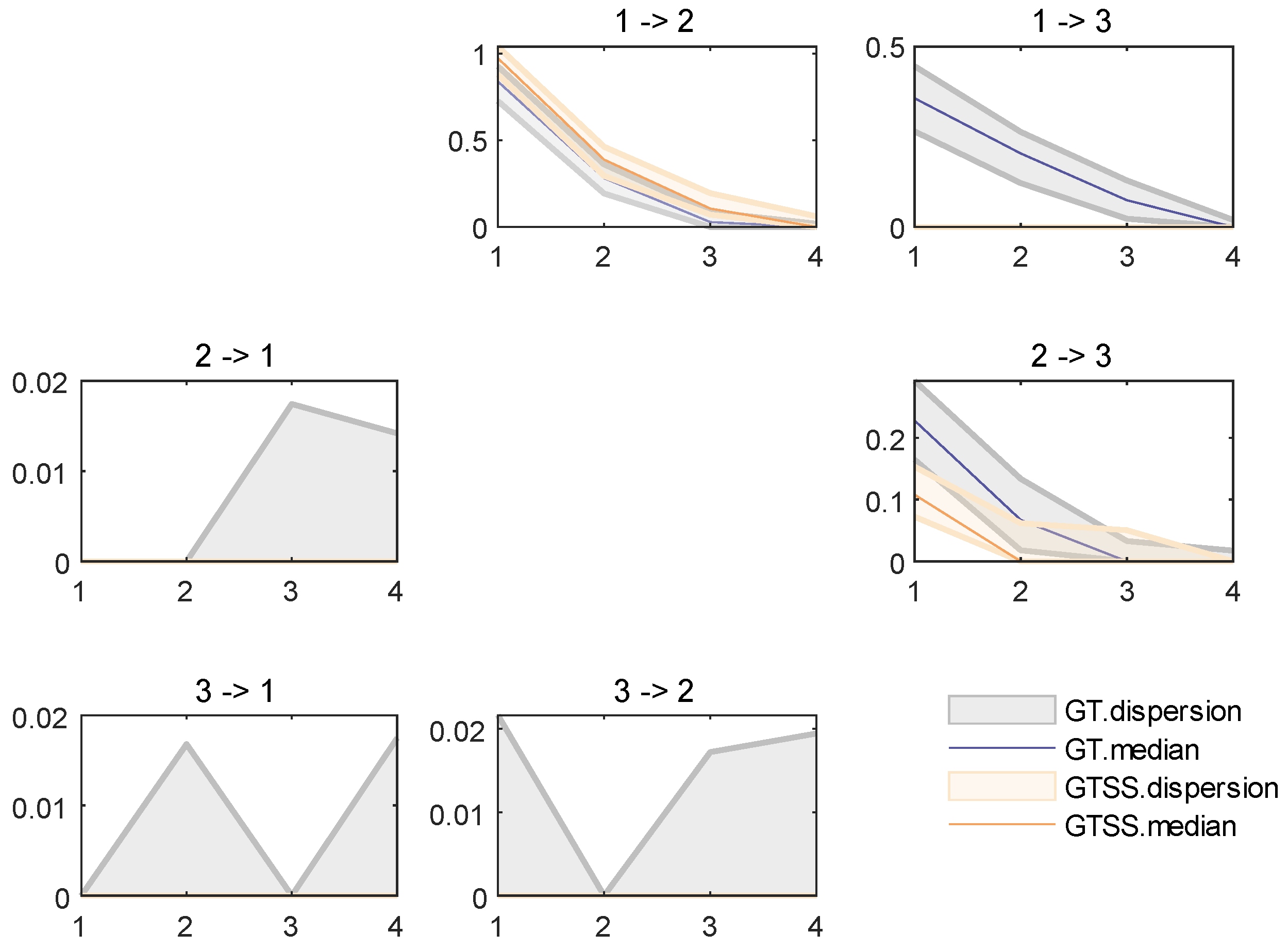
The results of 100 trials are shown in Figure 2 as an example. The GTSS method only generated GC values on $x_1\to x_2$ and $x_2\to x_3$ where Granger causality are truly present, whereas the GT method generated Granger causality under all combinations of variables, some of which are spurious.

The dispersion in this picture reflects the 90 percent confidence interval, while the median represents the median Granger causality value of 100 trials.

3.3. Example 2: Bivariate Series System

Next, a VAR(1) model is analysis which has the following structure,

$$\left[\begin{array}{c}{x}_t\\ y_t\end{array}\right]=A\left[\begin{array}{c}{x}_{t-1}\\ y_{t-1}\end{array}\right]+\left[\begin{array}{c}{\omega }_{1,t}\\ {\omega }_{2,t}\end{array}\right]$$

where $A=\left[\begin{array}{cc}0.4& 0.8\\ 0& 0.5\end{array}\right]$, hence the model has the Granger causality from y to x.

According to Equation (6) [34], the theoretical Granger causality value in $scale=1$ is 0.5578.

$$F_{y\to x}=ln\left(\frac{1+A_{22}^2+A_{12}^2+\sqrt{(1+A_{22}^2+A_{12}^2)-4A_{22}^2}}{2}\right)$$

(6)

Then 100 realization with ${10}^4$ nobs are generated according to VAR(1) model. The Granger causality of the model is estimated using the GT and GTSS methods respectively and the results are shown in

Table 3. Comparison between GT and GTSS with the results of 100 trials.

Method	Accuracy	ORR	MSE
GT	0.869	0.284	0.252
GTSS	0.998	0.003	0.002

, where MSE is the mean square error at $scale=1$. Based on the results in Table 3, it is clear that the GTSS method outperforms the GT method for all three indicators.

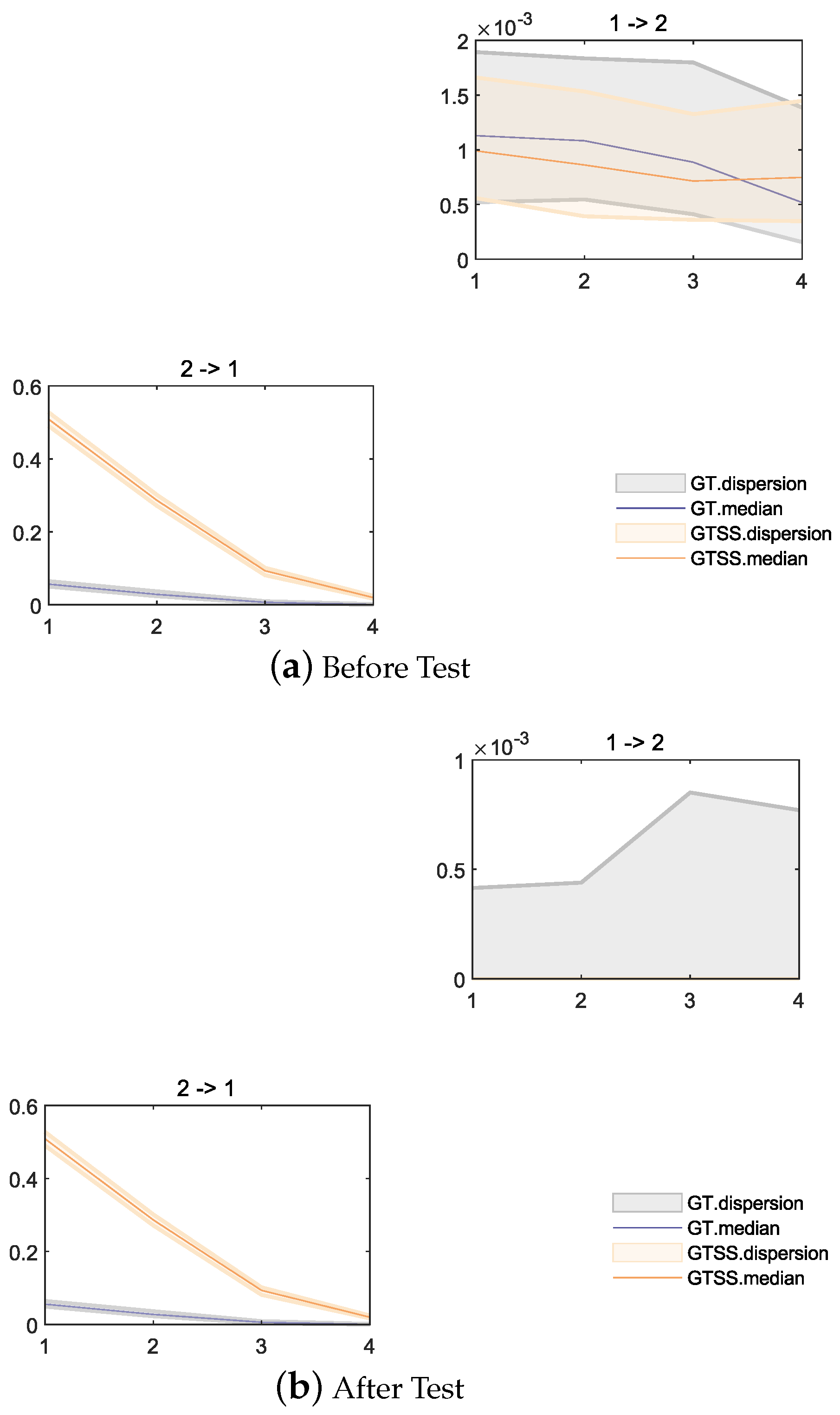
The scale—GC plots were plotted before and after hypothesis testing in Figure 3. From Figure 3a, the estimates of both methods were small in the direction of no causality, which is the 1 to 2 direction in the picture. After the hypothesis testing shown in Figure 3b, GTSS could obtain the correct causality relationship, but GT still had individual spurious causality. In addition, GTSS yields GC estimates that are close to the theoretical values, while GT estimates are considerably smaller than GTSS and the theoretical values on several scales.

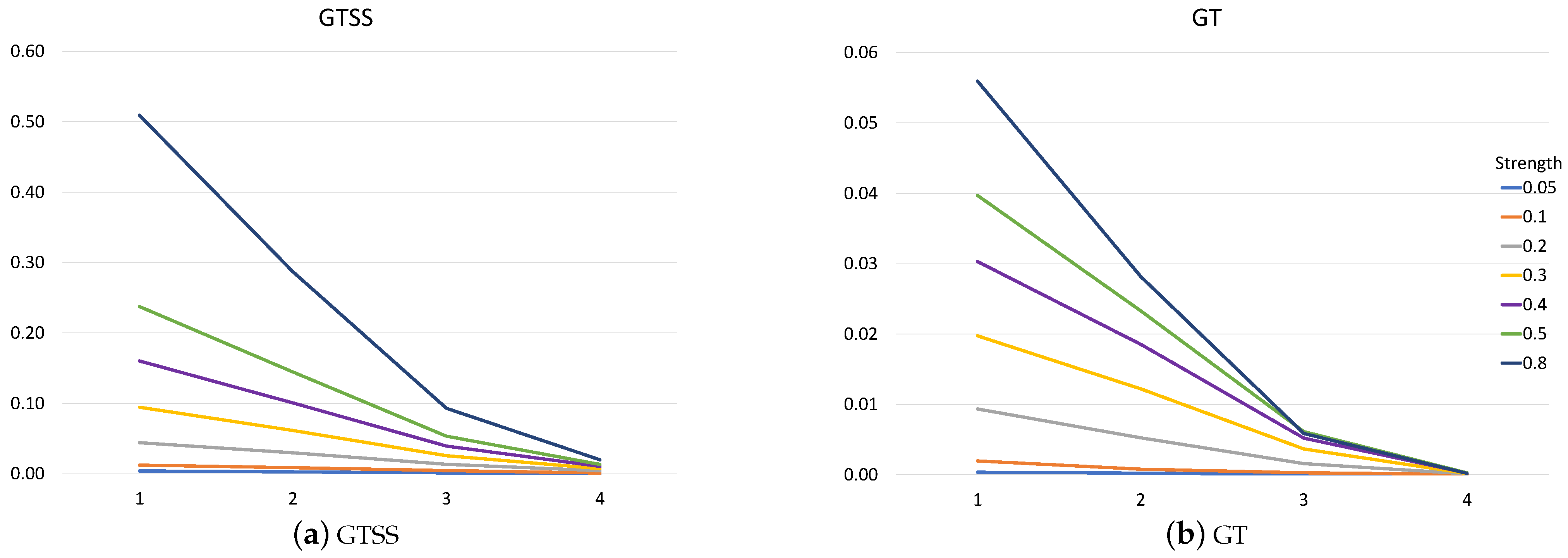
We plotted scale—GC plots in Figure 4 in order to explore the relationship between causal strength and the GC value by varying the $A(2,1)$ term in the coefficient matrix A, which is the causal strength of $y\to x$. The GC value displayed in the figure corresponds to the mean value obtained after 100 trials. The results demonstrated that the GC values obtained using both methods increased as the value of causality strength increased, eventually reaching a maximum value at the lag of 1.

The MSE of the GC values for both methods at $scale=1$ is compared in

Table 4. The MSE with different causal strength. ${\mathrm{MSE}}_{\mathrm{GTSS}}$ means the MSE using GTSS method, and MSE${}_{GT}$ means the MSE using GT method.

Strength	MSE${}_{\mathit{GTSS}}$	MSE${}_{\mathit{GT}}$
0.05	0.0000	0.0000
0.1	0.0000	0.0001
0.2	0.0001	0.0018
0.3	0.0003	0.0081
0.4	0.0006	0.0236
0.5	0.0011	0.0527
0.8	0.0025	0.2519

. At minimal levels of causal strength, the MSE of both techniques is negligible in part due to comparatively low GC estimates and the absence of significant outliers in their estimations. Nevertheless, as causal strength heightens, the MSE concurrently escalates. In comparison to GT, the MSE remains consistently lower in GTSS, indicating its superior ability to restore Granger causality values.

4. Conclusions

System transformations exhibit a multi-timescale structure and possess localization properties in the time domain, resulting in fluctuations that transpire across multiple time scales. These attributes cannot be sufficiently scrutinized with conventional time domain Granger causality analyses. Such analyses rely on VAR models, which are vulnerable to noise and downsampling challenges, and lack the ability for multiscale analyses.

In this study, the GTSS approach, which analyzes Granger causality between multivariate time series on multiple time scales by combining the state space model with wavelet transform, is suggested. To be more precise, we first substitute the driving variable with the result of the wavelet transform before incorporating the transform data into the state space model. The hypothesis test is carried out by calculating the residuals of the models. Finally, the Granger causality value and the relationship between the various factors may be determined.

The experimental results show that GTSS has better capability for multiscale Granger causality analysis than the GT method based on the VAR model. The comparative analysis between the two methods highlights the superior performance of GTSS in accurately identifying causal relationships, especially in situations where they are asymmetric in nature.

The relationship between model order, number of trials and strength of causality and Granger causality is investigated. Our results reveal that the causality value decreases at higher time scales, while the accuracy improves with an increase in the number of trials, providing valuable insights for future studies to select appropriate parameter settings for these parameters, thereby enhancing the accuracy of Granger causality analyses.

Furthermore, the multiscale analysis using empirical model methods provides a better view of the underlying driving variables according to He K. et al. [35]. Deep learning has been effectively applied to the study of Granger causality to determine causal linkages in complicated systems [36]. Therefore, future study could examine data processing in conjunction with empirical modal decomposition or employ different deep learning models for modeling time series.