The Discrete Exponentiated-Chen Model and Its Applications

Abstract

A novel discrete exponentiated Chen (DEC) distribution, which is a subset of the continuous exponentiated Chen distribution, is proposed. The offered model is more adaptable to analyzing a wide range of data than traditional and recently published models. Several important statistical and reliability characteristics of the DEC model are introduced. In the presence of Type-II censored data, the maximum likelihood and asymptotic confidence interval estimators of the model parameters are acquired. Two various bootstrapping estimators of the DEC parameters are also obtained. To examine the efficacy of the adopted methods, several simulations are implemented. To further clarify the offered model in the life scenario, the two applications, based on the number of vehicle fatalities in South Carolina in 2012 and the final exam marks in 2004 at the Indian Institute of Technology at Kanpur, are analyzed. The analysis findings showed that the DEC model is the most effective model for fitting the supplied data sets compared to eleven well-known models in literature, including: Poisson, geometric, negative binomial, discrete-Weibull, discrete Burr Type XII, discrete generalized exponential, discrete-gamma, discrete Burr Hatke, discrete Nadarajah-Haghighi, discrete modified-Weibull, and exponentiated discrete-Weibull models. Ultimately, the new model is recommended to be applied in many fields of real practice.

1. Introduction

When it becomes impossible or impracticable to evaluate a product’s or piece of equipment’s lifespan on a continuous scale, the discretization phenomenon occurs. This applies to many domains, including clinical trials, engineering, economics, and other associated sciences; see [1]. The lifespan of a copy machine is determined by the total number of copies it produces. In survival analysis, the lifetime periods for people with brain tumors, or the duration between remission and recurrence, may be documented as the number of days. In a reliability framework, the functional state of a system is checked every unit of time. Observed statistics represent the number of time units achieved prior to a failure. In addition to lifespan statistics, the count phenomenon may be seen in a variety of real-world contexts, including the number of earthquakes in a year, accidents, ecological species types, insurance claims, and more. Discrete distributions are quite helpful for modeling lifespan data in such circumstances. In this situation, the geometric and negative binomial distributions are recognized as discrete substitutes for the exponential and gamma distributions. In some real-world circumstances, these distributions do not, however, fit discrete data. Many continuous lifespan distributions have been discretized in the literature in recent decades as a result of the demand for more believable discrete distributions to simulate discrete data in a range of real-world settings.

Consider the discrete Weibull distribution, which is discussed in refs. [2,3], the discrete Rayleigh distribution, which is discussed in refs. [4,5], the discrete inverse, which is discussed in ref. [6], the exponentiated discrete Weibull distribution in ref. [7], and the discrete Weibull geometric distribution, see [8]. To simulate data with a bathtub shape and a growing failure rate in recent years, ref. [9] developed a discrete additive Perks-Weibull distribution. The discrete Nadarajah and Haghighi distributions for one variable were initially proposed by ref. [10]. To evaluate discrete rising failure and count data, ref. [11] presented a discrete Perks distribution. A brand-new discrete Lindley distribution with two parameters and an unusual bathtub-shaped hazard rate characteristic was described by ref. [12]. For over- and under-dispersed data, ref. [13] presents the discrete Gompertz-G family. Ref. [14] estimated the quantity of new coronavirus cases using a discrete generalized Lindley distribution. A discrete equivalent of the peculiar Weibull-G family of distributions was shown by ref. [15]. They spoke about traditional and Bayesian estimates and showed how the suggested model may be used with count data sets. A discrete equivalent of the Teissier distribution with application to data counting was recently studied by ref. [16].

Even though there are a lot of discretized distributions in the literature, there could be situations when they conflict with discrete data modeling. There is therefore still plenty of potential for creating novel discretized distributions that are appropriate in various situations. In light of this, we suggest a discretized variant of the exponentiated Chen distribution proposed by ref. [17]. To discretize continuous distribution, a variety of techniques can be applied; see [18]. The following is the most typical procedure for finding the discrete analog of a continuous distribution. Many discrete distributions have been introduced using this approach to discretization, including the natural discrete Lindley [19], the discrete Marshal-Olkin Weibull [20], the uniform Poisson-Ailamujia [21], the discrete inverted Topp-Leone [22], and the discrete power-Ailamujia [23].

If the underlying random variable (RV) $X$ has the survival function (SF), $S_X\left(x\right)P(X\ge x)$, the underlying RV $Y$ has the probability mass function (PMF) ($Y=\left[X\right]$, biggest integer less than or equal to $X$)

$$\begin{array}{ll}P\left(Y=y\right)& =P\left(y\le X<y+1\right)\\ & =P\left(X\ge y\right)-P\left(X\ge y+1\right)=S_X\left(y\right)-S_X\left(y+1\right),y=\mathrm{0,1},2,\dots ,\infty .\end{array}$$

(1)

The technique described above generates a discrete distribution by using the same functional form as the continuous version of the SF. However, this discrete variant retains certain aspects of dependability. There is a strong motivation to apply this technique in order to create discrete versions of existing continuous distributions. On numerous occasions, constraints such as limited time or resources hinder the collection of complete data sets. Incomplete data can involve censored data, which can be further explored in ref. [24]. Various censoring algorithms have been documented in the literature to analyze these types of data sets. The commonly employed censoring techniques include Type I and Type II censoring. Type I censoring involves recording the event only if it occurs before a predetermined time, while Type II censoring continues the research until a specific number of subjects experience failure. Random censoring, on the other hand, is a distinct type of censorship where individuals can be censored at any point during the experiment and at different time intervals. In the context of clinical trials or medical research, random censorship could occur when patients withdraw early without completing the prescribed treatment. Further information on censoring techniques, their extensions, and their analysis can be found in ref. [25]. Accurate analysis of randomly censored lifespan data is crucial to derive reliable insights and meaningful research findings. Such data sets are frequently encountered in fields such as biology, reliability studies, and medical science. Typically, these data involve right-censoring, as it is impractical to observe individuals until their deaths or because participants may drop out of the study. In regard to right-censoring with discrete observations, it has been examined by [26]. Notably, ref. [27] investigated various inferential approaches for the exponentiated discrete Weibull model with censored data.

Therefore, the main objectives of the DEC model are:

• The first advantage of this distribution over many other one- or two-parameter discrete distributions is that it gives the various hazard rate forms, such as decreasing, increasing, or increasing-constant. So, by virtue of these hazard rates, the proposed model is suitable for modeling various data sets;
• It offers various PMF shapes that may not be adequately modeled by other competitive models that are appropriate to model positively skewed, negatively skewed, or symmetric data;
• Several statistical and reliability characteristics, including moments, probability functions, reliability indices, hazard functions, order statistics, etc., are introduced;
• Analysis results from two real applications showed that the DEC distribution fits the given data sets satisfactorily compared to the other eleven discrete distribution models in the literature;
• Maximum likelihood and bootstrapping estimation methods are considered to estimate the proposed parameters in the presence of data collected under the Type-II censored strategy;
• Through extensive Monte Carlo simulations using various accuracy criteria, namely mean squared errors, mean absolute biases, and average interval lengths, the performance of the acquired estimators is evaluated. It may seem reasonable to recommend the use of Type-II censoring for estimating unknown parameters.

The remainder of the paper is organized as follows: In Section 2, materials and methods are provided. Monte Carlo results and real data analysis are illustrated in Section 3 and Section 4, respectively. Finally, we provide some concluding remarks in Section 5.

2. Materials and Methods

The SF of the continuous exponentiated Chen distribution is provided by:

$$S\left(x\right)=1-{\left(1-e^{\beta \left(1-e^{x^{\lambda }}\right)}\right)}^{\theta },\beta ,\lambda ,\theta >0,x\ge 0,$$

(2)

subsequently, the PMF of the DEC distribution becomes

$$P\left(x\right)={\left(1-e^{\beta \left(1-e^{{\left(x+1\right)}^{\lambda }}\right)}\right)}^{\theta }-{\left(1-e^{\beta \left(1-e^{x^{\lambda }}\right)}\right)}^{\theta },x=\mathrm{0,1},2,\dots ,\infty ,$$

(3)

where $\beta ,\lambda ,\theta >0,$ are the shape parameters. It is easy to show that the PMF in Equation (3) is accurate, i.e., $\sum _{x=0}^{\infty }P\left(X=x\right)=1$.

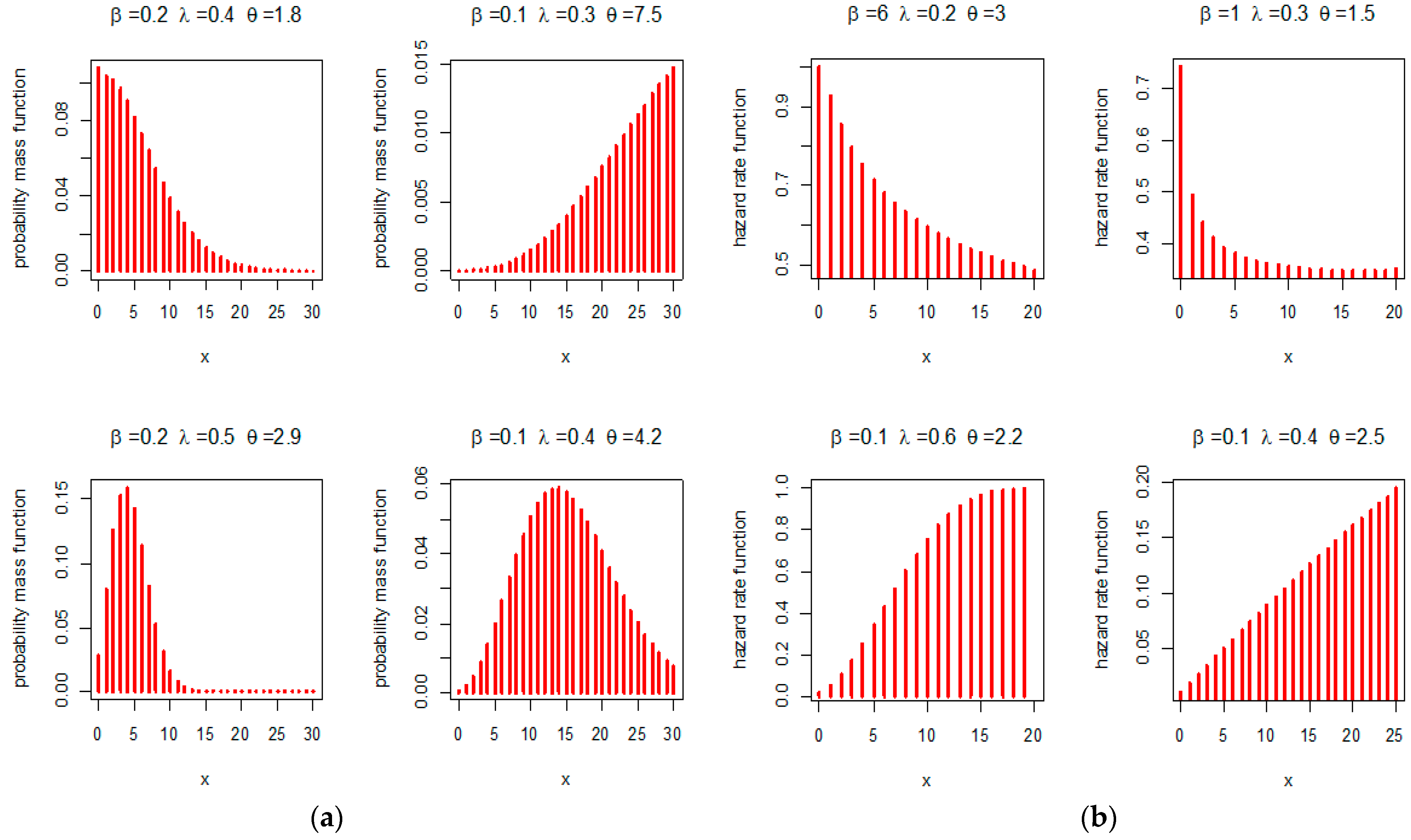
For specified values of $\beta ,$ $\lambda ,$ and $\theta$ based on their domains, Figure 1 displays the PMF and hazard rate function (HRF) shapes of the DEC distribution. It shows that the PMF can be unimodal (for $\beta =0.1,$ $\lambda =0.4,$ $\theta =4.2$), right skewed (for $\beta =0.2,$ $\lambda =0.4,$ $\theta =1.8$) or left skewed (for $\beta =0.1,$ $\lambda =0.3,$ $\theta =7.5$). It also shows that the HRF of the new model exhibits different shapes, such as the decreasing (for $\beta =6,$ $\lambda =0.2,$ $\theta =3$), increasing (for $\beta =0.1,$ $\lambda =0.6,$ $\theta =2.2$) or increasing-constant (for $\beta =0.1,$ $\lambda =0.4,$ $\theta =2.5$). As a result, the proposed model is suitable for modeling different real-world data sets.

For PMF in Equation (3), the cumulative distribution function (CDF) of DEC is given by:

$$F\left(x\right)=\left\{\begin{array}{ll}{\left[1-e^{\beta \left\{1-e^{(\lfloor x\rfloor +1{)}^{\lambda }}\right\}}\right]}^{\theta }& for x\ge 0\\ 0& for x<0\end{array}\right.$$

(4)

where $\lfloor x\rfloor$ is the floor function that gives the greatest integer less than or equal to $x$. Then the quantile function can be defined as $Q\left(y\right)=inf\{x:F(x)\ge y\}.$ For more details on this quantile function, see Section 14 of ref. [28] and Theorem 2.1.10 of ref. [29]. It should be noted here that $F\left(0\right)={\left(1-e^{\beta \left(1-e\right)}\right)}^{\theta },$ and the proportion of non-zero values is given by $1-F\left(0\right).$

Lemma 1. 

Let $\lfloor x\rfloor$ denote the floor function and let ⌈x⌉ be a ceiling operator that provides the least number larger (or equal to) than x. Then, for any integer $n$ (or m), and real number $x$, we have the following:

(i) 

$n\ge x$ if and only if $n\ge \lceil x\rceil$.

(ii) 

$\lfloor x\rfloor \ge m$ if and only if $x\ge m$.

Proof. 

According to ref. [30],

(i)

Since $\lceil x\rceil \ge x$, $n\ge \lceil x\rceil$ implies $n\ge ⌈x⌉\ge x$. Thus, we have $n\ge x$. Next, we need to prove that $n\ge x$ implies $n\ge \lceil x\rceil$. Its contrapositive statement is that $n<\lceil x\rceil$ implies $n<x$. Since $\lceil x\rceil -1<x\le \lceil x\rceil$, we can rewrite $\lceil x\rceil =x+\delta$, where $0\le \delta <1$. Since $n$ and $\lceil x\rceil$ are both integers, it is immediate from $n<\lceil x\rceil$ that we can set $n=\lceil x\rceil -k$ where $k=\mathrm{1,2},\dots$. If we assume that $n<x$ is not satisfied (that is, $n\ge x$), then we have $\lceil x\rceil -k\ge x$ which results in $\delta =\lceil x\rceil -x\ge k$. Thus, we have $\delta \ge 1$ since $k=\mathrm{1,2},\dots$, which violates the condition $0\le \delta <1$.

(ii)

Since $x\ge \lfloor x\rfloor$, we have $x\ge m$ if $\lfloor x\rfloor \ge m$. Next, we need to prove that $x\ge m$ implies $\lfloor x\rfloor \ge m$. Its contrapositive statement is that $\lfloor x\rfloor <m$ implies $x<m$. Since $\lfloor x\rfloor \le x<\lfloor x\rfloor +1$, we can rewrite $\lfloor x\rfloor =x-\delta$, where $0\le \delta <1$. Since $m$ and $\lfloor x\rfloor$ are both integers, it is immediate from $\lfloor x\rfloor <m$ that we can set $m=\lfloor x\rfloor +k$ where $k=\mathrm{1,2},\dots$. If we assume that $x<m$ is not satisfied (that is $x\ge m$), then we have $x\ge \lfloor x\rfloor +k$, which results in $\delta =x-\lfloor x\rfloor \ge k$. Thus, we have $\delta \ge 1$, which violates the condition $0\le \delta <1$. □

However, the quantile function, $Q\left(y\right)=F^{-1}\left(y\right)$, of the DEC distribution is given by

$$Q\left(y\right)=⌈{\left\{ln\left(1-\frac{1}{\beta }ln(1-y^{1/\theta })\right)\right\}}^{1/\lambda }-1⌉.$$

Proof. 

It is immediate from $F\left(x\right)\ge y$ that we have

$$\lfloor x\rfloor \ge {\left\{ln\left(1-\frac{1}{\beta }ln(1-y^{1/\theta })\right)\right\}}^{1/\lambda }-1$$

(5)

Since $\lfloor x\rfloor$ is an integer, we denote $n=\lfloor x\rfloor$ for notational convenience. Then, applying Lemma 1(i) to (1), we know that $F\left(x\right)\ge y$ is equivalent to

$$\lfloor x\rfloor \ge ⌈{\left\{ln\left(1-\frac{1}{\beta }ln(1-y^{1/\theta })\right)\right\}}^{1/\lambda }-1⌉$$

(6)

Since the last term in Equation (6) is an integer, we denote

$$m=⌈{\left\{ln\left(1-\frac{1}{\beta }ln(1-y^{1/\theta })\right)\right\}}^{1/\lambda }-1⌉,$$

(7)

for notational convenience. That is, we have $\lfloor x\rfloor \ge m$. By applying Lemma 1(ii), we have $x\ge m$, which implies

$$x\ge ⌈{\left\{ln\left(1-\frac{1}{\beta }ln(1-y^{1/\theta })\right)\right\}}^{1/\lambda }-1⌉$$

(8)

Then $F\left(x\right)\ge y$ is equivalent to

$$x\ge ⌈{\left\{ln\left(1-\frac{1}{\beta }ln(1-y^{1/\theta })\right)\right\}}^{1/\lambda }-1⌉.$$

(9)

Thus, we have

$$\begin{array}{ll}Q\left(y\right)& =inf\{x:F(x)\ge y\}\\ & =inf\left\{x:x\ge ⌈{\left\{ln\left(1-\frac{1}{\beta }ln(1-y^{1/\theta })\right)\right\}}^{1/\lambda }-1⌉\right\}\\ & =⌈{\left\{ln\left(1-\frac{1}{\beta }ln(1-y^{1/\theta })\right)\right\}}^{1/\lambda }-1⌉,\end{array}$$

(10)

which completes the proof. It is noteworthy that the quantile function is left-continuous while the CDF is right-continuous ref. [31]. □

2.1. Statistical Properties

2.1.1. Random Number Generation, Skewness, and Kurtosis

The popular quantile-based formulae for skewness or kurtosis were established by refs. [32,33]. These indicators stand out in part because they can be computed even for distributions lacking moments and are less impacted by outliers. Following ref. [32], the skewness ($Sk$) can be expressed as:

$$Sk=\frac{Q\left(\frac{3}{4}\right)+Q\left(\frac{1}{4}\right)-2Q\left(\frac{1}{2}\right)}{Q\left(\frac{3}{4}\right)-Q\left(\frac{1}{4}\right)}.$$

(11)

The Moors kurtosis [33], denoted by $Ku$, suggests looking like this:

$$Ku=\frac{Q\left(\frac{7}{8}\right)-Q\left(\frac{5}{8}\right)+Q\left(\frac{3}{8}\right)-Q\left(\frac{1}{8}\right)}{Q\left(\frac{3}{4}\right)-Q\left(\frac{1}{4}\right)}.$$

(12)

Using Equation (5) in the aforementioned formulas, it is simple to derive the $Sk$ and $Ku$ for the DEC distribution.

2.1.2. Moments

Calculating a probability distribution’s mean, variance, $Sk$, $Ku$, and other properties involves using the distribution’s moments. The $r\mathrm{th}$ raw moments of the DEC distribution may be obtained as follows:

$$\begin{array}{ll}{\stackrel{`}{\omega }}_r& =E\left(X^r\right)={\displaystyle \sum _x}\left({\left(x+1\right)}^r-x^r\right)\left(1-F\left(x\right)\right)\\ & ={\displaystyle \sum _x}\left({\left(x+1\right)}^r-x^r\right)\left(1-{\left(1-e^{\beta \left(1-e^{x^{\lambda }}\right)}\right)}^{\theta }\right).\end{array}$$

(13)

Hence, following [9], the DEC distribution’s initial four raw moments are obtained by substituting $r=\mathrm{1,2},\mathrm{3,4}$ using Equation (13).

Using the raw moments from the following relations, we can quickly determine the $Sk$ and $Ku$ as follows:

$$Sk=\frac{{\stackrel{`}{\omega }}_3-3{\stackrel{`}{\omega }}_2{\stackrel{`}{\omega }}_1+2{\stackrel{`}{\omega }}_1^3}{{\left[V\left(X\right)\right]}^{3/2}} \mathrm{a}\mathrm{n}\mathrm{d} Ku=\frac{{\stackrel{`}{\omega }}_4-4{\stackrel{`}{\omega }}_2{\stackrel{`}{\omega }}_1+6{\stackrel{`}{\omega }}_2{\stackrel{`}{\omega }}_1^2-3{\stackrel{`}{\omega }}_1^4}{{\left[V\left(X\right)\right]}^2}.$$

The ratio of the standard deviation to the mean is known as the coefficient of variation ($CV$). The variance-to-mean ratio serves as the index of dispersion ($ID$). Keep in mind that the $CV$ is always scale-invariant and dimensionless. The $ID$, on the other hand, is only dimensionless when it pertains to a dimensionless quantity, such as a count, as is the case in practice. It is not scale-invariant.

Although both $CV$ and $ID$ are for non-negative variables, they are applied in various situations. Most frequently, discrete variables with non-negative integer values, like counts, are represented by the sample and theoretical $ID$s. A method for detecting whether data is uniformly, unequally, or overly spread is the in $ID$, such as $ID>1,$ which refers to over-dispersion, $ID<1;$ refers to the opposite (under-dispersion), and $ID=1$ refers to equi-dispersion. The following is the $ID$ for the DEC model:

$$ID=\frac{V\left(X\right)}{E\left(X\right)},$$

(14)

where $V\left(X\right)$ and $E\left(X\right)$ are the variance and mean of $X$, respectively.

If one needs to compare the variance of two independent samples, the coefficient of variation ($CV$), which is a relative measure of variance, is usually applied. Greater variability is indicated by a high $CV$ value. However, the $CV$ for the DEC distribution is given by

$$CV=\frac{{V\left(X\right)}^{0.5}}{E\left(X\right)}.$$

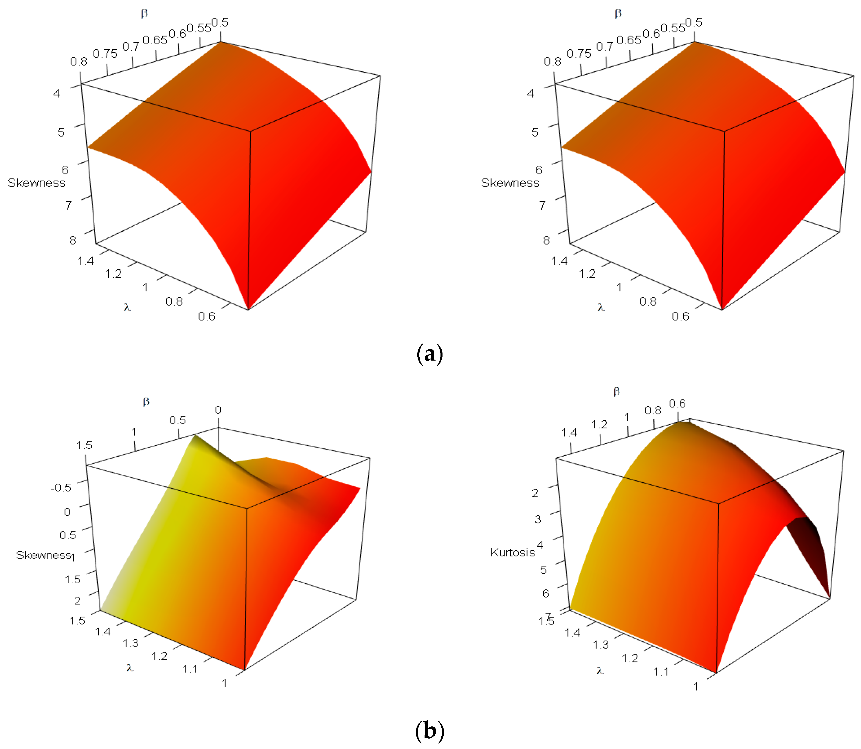
The aforementioned equations do not have a closed form, so we utilize R software to statistically illustrate these traits. Figure 2 displays some shapes of the $Sk$ and $Ku$ measures of the proposed model. It indicates that both measures depend excessively on the values of $\theta$. Using a complete random sample of size $n=100$, based on different combinations of DEC parameters,

Table 1. Some statistics for the DEC distribution using different combinations of its parameters.

$\mathit{\lambda }\to$		0.1				0.5				1.5
$\mathit{\beta }\downarrow$	$\mathit{\theta }\to$	1	2	3	4	1	2	3	4	1	2	3	4
1	$M$	2.3207	4.4133	6.3008	8.0035	0.2353	0.4364	0.6091	0.7582	0.1794	0.3266	0.4474	0.5465
	$V$	95.134	174.98	242.48	300.02	0.3193	0.5202	0.6432	0.7153	0.1472	0.2199	0.2472	0.2478
	$ID$	40.994	39.648	38.485	37.486	1.3567	1.1922	1.0561	0.9434	0.8206	0.6734	0.5526	0.4535
	$CV$	4.2030	2.9973	2.4714	2.1642	2.4012	1.6529	1.3168	1.1155	2.1389	1.4360	1.1114	0.9110
	$Sk$	6.0441	4.2406	3.4390	2.9609	2.8412	1.8383	1.3848	1.1212	1.6714	0.7396	0.2117	0.1868
	$Ku$	50.638	29.624	23.037	20.042	15.984	11.555	11.543	12.958	3.7936	1.5471	1.0449	1.0350
2	$M$	0.2281	0.4534	0.6761	0.8961	0.0342	0.0675	0.0997	0.1309	0.0322	0.0633	0.0935	0.1226
	$V$	6.5340	12.941	19.226	25.391	0.0374	0.0716	0.1027	0.1310	0.0311	0.0593	0.0847	0.1076
	$ID$	28.649	28.542	28.438	28.335	1.0923	1.0609	1.0306	1.0012	0.9678	0.9367	0.9065	0.8774
	$CV$	11.208	7.9341	6.4856	5.6232	5.6477	3.9660	3.2159	2.7659	5.4845	3.8463	3.1146	2.6749
	$Sk$	20.610	14.585	11.918	10.329	6.0767	4.1707	3.3025	2.7712	5.3022	3.5863	2.7935	2.3011
	$Ku$	546.12	278.22	188.98	144.40	45.191	22.825	15.456	11.843	29.113	13.862	8.8037	6.2950
3	$M$	0.0230	0.0459	0.0688	0.0917	0.0059	0.0117	0.0175	0.0232	0.0058	0.0115	0.0172	0.0229
	$V$	0.3840	0.7668	1.1483	1.5286	0.0060	0.0119	0.0177	0.0234	0.0057	0.0114	0.0169	0.0224
	$ID$	16.695	16.688	16.681	16.674	1.0247	1.0190	1.0133	1.0076	0.9942	0.9885	0.9828	0.9771
	$CV$	26.940	19.057	15.566	13.486	13.224	9.3376	7.6135	6.5844	13.125	9.2674	7.5559	6.5341
	$Sk$	66.288	46.906	38.325	33.214	13.533	9.5060	7.7100	6.6323	13.049	9.1595	7.4235	6.3810
	$Ku$	6359.3	3189.8	2133.3	1605.1	194.29	96.648	64.106	47.841	171.27	84.897	56.108	41.717

displays some numerical findings for the mean ($M$), variance ($V$), $ID$, $CV$, $Sk$, and $Ku$ of the DEC distribution and indicates that:

• For fixed $\beta$ and $\theta$, as $\lambda$ increases, the values of $M$, $V$, $ID$, $CV$, $Sk$, and $Ku$ decrease;
• For fixed $\beta$ and $\lambda$, as $\theta$ increases, the values of $M$ and $V$ increase, whereas $ID$, $CV$, $Sk$, and $Ku$ decrease;
• For fixed $\theta$ and $\lambda$, as $\beta$ increases, the values of $M$, $V$, and $ID$ decrease, whereas $CV$, $Sk$, and $Ku$ increase.

2.1.3. Survival and Hazard Rate Functions

The DEC distribution’s SF ($S(·)$) and HRF ($h(·)$) are provided, respectively, by

$$S\left(x\right)=P\left(X\ge x\right)=1-{\left(1-e^{\beta \left(1-e^{x^{\lambda }}\right)}\right)}^{\theta },x=\mathrm{0,1},2,\dots ,\infty ,$$

(15)

and

$$h\left(x\right)=P\left(X=x|X\ge x\right)=\frac{{\left(1-e^{\beta \left(1-e^{{\left(x+1\right)}^{\lambda }}\right)}\right)}^{\theta }-{\left(1-e^{\beta \left(1-e^{x^{\lambda }}\right)}\right)}^{\theta }}{1-{\left(1-e^{\beta \left(1-e^{x^{\lambda }}\right)}\right)}^{\theta }},x=\mathrm{0,1},2,\dots ,\mathrm{\infty }.$$

(16)

The recommended distribution is more flexible to evaluate a broad range of data than conventional and recently published models as a result of the distinctive forms of HRF. The second rate of hazard (symbolized by $srh\left(·\right)$) and reversed hazard rate (symbolized by $rhr\left(·\right)$) function of the suggested model are also explored.

$$srh\left(x\right)=P\left(X=x|X\le x\right)=\frac{{\left(1-e^{\beta \left(1-e^{{\left(x+1\right)}^{\lambda }}\right)}\right)}^{\theta }-{\left(1-e^{\beta \left(1-e^{x^{\lambda }}\right)}\right)}^{\theta }}{{\left(1-e^{\beta \left(1-e^{{\left(x+1\right)}^{\lambda }}\right)}\right)}^{\theta }},x=\mathrm{0,1},2,\dots ,\mathrm{\infty },$$

(17)

and

$$rhr\left(x\right)=ln\left[\frac{S\left(x\right)}{S\left(x+1\right)}\right]=ln\left[\frac{1-{\left(1-e^{\beta \left(1-e^{x^{\lambda }}\right)}\right)}^{\theta }}{1-{\left(1-e^{\beta \left(1-e^{{\left(x+1\right)}^{\lambda }}\right)}\right)}^{\theta }}\right],x=\mathrm{0,1},2,\dots ,\mathrm{\infty }.$$

(18)

2.1.4. Mean Past Life Function

The predicted inactivity time function, also known as the mean-past-life (MPL) function, is symbolised by the sign $m^{\mathrm{*}}\left(i\right)$ and it measures the amount of time that has elapsed since $X$ failed, presuming that the system failed before $i$. It has various uses, including actuarial studies, the dependability concept, survival evaluation, and forensic science. In a discrete setting, the MPL function is defined as:

$$m^{*}\left(i\right)=E\left(i-X|X<i\right)=\frac{1}{F\left(i-1\right)}{\sum }_{j=1}^{i}F\left(j-1\right);i=\mathrm{1,2},3,\dots ,\mathrm{\infty }.$$

(19)

By substituting Equation (4) into $m^{\mathrm{*}}\left(i\right)$, we can quickly calculate the MPL for the suggested model.

2.1.5. Stress-Strength Reliability

Stress-strength (SS) reliability describes the life of a component that has random strength (say $X$) and is subjected to a random stress (say $Z$). The component fails when the stress applied to it exceeds its strength, but it continues to operate satisfactorily whenever $R=P[X>Z]$. If the applied stress is greater than the component’s strength, it instantly fails; otherwise, it performs properly. The SS system paradigm has several uses in disciplines including engineering, medicine, psychology, and other related domains; see [34,35,36,37]. A thorough analysis of SS models is provided in ref. [38]. For discrete independent RVs $X$ and $Z$, the SS reliability is defined as:

$$R=P\left(X>Z\right)={\sum }_{x=0}^{\infty }{P}_X\left(x\right)F_Z\left(x\right),$$

where, respectively, $P_X\left(x\right)$ and $F_Z\left(x\right)$ stand for the PMF and CDF of the independent discrete RVs, $X$ and $Z$. Let the numbers $X~DEC({\beta }_1,{\lambda }_1,{\theta }_1)$ and $X~DEC({\beta }_2,{\lambda }_2,{\theta }_2)$ be genuine. Next, using Equations (3) and (4), we get

$$R={\sum }_{x=0}^{\infty }\left[{\left(1-e^{{\beta }_1\left(1-e^{{\left(x+1\right)}^{{\lambda }_1}}\right)}\right)}^{{\theta }_1}-{\left(1-e^{{\beta }_1\left(1-e^{x^{{\lambda }_1}}\right)}\right)}^{{\theta }_1}\right]{\left(1-e^{{\beta }_2\left(1-e^{{\left(x+1\right)}^{{\lambda }_2}}\right)}\right)}^{{\theta }_2}.$$

(20)

Since the SS reliability parameter cannot be expressed in a clear formula, it can be easily evaluated via any software.

2.1.6. Order Statistics

Particularly in the study of survival, order statistics are critical for constructing tolerance ranges for distributions and identifying population features. Let $X_1,X_2,...,X_n$ represent a sample of size, $n$, taken at random sample from the DEC$\left(\beta ,\lambda ,\theta \right)$. Let the associated order statistics be represented by $X_{\left(1\right)},X_{\left(2\right)},...,X_{\left(n\right)}$. The CDF of the $r\mathrm{th}$ order statistic is thus provided by, let’s say, $\upsilon ={\mathrm{X}}_{\left(r\right)}$ as:

$$\begin{array}{ll}{F}_r\left(\upsilon \right)=& {\sum }_{i=r}^n\left(\begin{array}{c}n\\ i\end{array}\right)F^i\left(\upsilon \right){\left[1-F\left(\upsilon \right)\right]}^{n-i}\\ & ={\sum }_{i=r}^n{\sum }_{k=0}^{n-i}{\left(-1\right)}^k\left(\begin{array}{c}n\\ i\end{array}\right)\left(\begin{array}{c}n-i\\ k\end{array}\right)F^{i+k}\left(\pi \upsilon \right)\\ & ={\sum }_{i=r}^n{\sum }_{k=0}^{n-i}{\left(-1\right)}^k\left(\begin{array}{c}n\\ i\end{array}\right)\left(\begin{array}{c}n-i\\ k\end{array}\right){\left[{\left(1-e^{\beta \left(1-e^{{\left(x+1\right)}^{\lambda }}\right)}\right)}^{\theta }\right]}^{i+k}.\end{array}$$

(21)

The corresponding PMF for $r\mathrm{th}$ order statistic is

$$\begin{array}{ll}{F}_r\left(\upsilon \right)& =F_r\left(\upsilon \right)-F_r\left(\upsilon -1\right)\\ & ={\sum }_{i=r}^n{\sum }_{k=0}^{n-i}{\left(-1\right)}^k\left(\begin{array}{c}n\\ i\end{array}\right)\left(\begin{array}{c}n-i\\ k\end{array}\right){\left[{\left(1-e^{\beta \left(1-e^{{\left(\upsilon +1\right)}^{\lambda }}\right)}\right)}^{\theta }\right]}^{i+k}\\ & -{\sum }_{i=r}^n{\sum }_{k=0}^{n-i}{\left(-1\right)}^k\left(\begin{array}{c}n\\ i\end{array}\right)\left(\begin{array}{c}n-i\\ k\end{array}\right){\left[{\left(1-e^{\beta \left(1-e^{{\left(\upsilon \right)}^{\lambda }}\right)}\right)}^{\theta }\right]}^{i+k}\end{array}$$

(22)

Setting $r=1$ or $r=n$ in Equation (9), the PMF of $\mathrm{m}\mathrm{i}\mathrm{n}\left(X_{\left(1\right)},\dots ,X_{\left(n\right)}\right)$ or $\mathrm{m}\mathrm{a}\mathrm{x}\left(X_{\left(1\right)},\dots ,X_{\left(n\right)}\right)$ can be easily obtained.

2.1.7. Entropy

The average amount of “information,” “surprise,” or “uncertainty” included in a RV’s probable outcomes is measured by its entropy, in accordance with the principles of information theory. The Renyi entropy (RE) (see [39]) is a fundamental entropy. It is a key measure of complexity and uncertainty in many fields, such as statistical inference, physics, econometrics, and pattern recognition in computer science. For the DEC distribution, the RE $(\mathrm{f}\mathrm{o}\mathrm{r} \rho >0,\rho \ne 1)$ can be specified as:

$$\begin{array}{ll}\mathrm{R}\mathrm{E}\left(\rho \right)& =\frac{1}{1-\rho }ln{\sum }_{x=0}^{\infty }{P}_x^{\rho }\left(x\right)\\ & =\frac{\rho }{1-\rho }ln{\sum }_{x=0}^{\infty }\left\{{\left(1-e^{\beta \left(1-e^{{\left(x+1\right)}^{\lambda }}\right)}\right)}^{\theta }-{\left(1-e^{\beta \left(1-e^{x^{\lambda }}\right)}\right)}^{\theta }\right\},\end{array}$$

(23)

where $\rho \in \mathbb{R}$ is a deformation parameter. As a specific instance of RE as $\rho \to 1$, Shannon entropy (Sh.E), which is given by $\mathrm{S}\mathrm{h}.\mathrm{E}=-E\left[lnP\right(X\left)\right]$, may be produced.

2.2. Maximum Likelihood Method

One of the most commonly used methods for classical point estimation is the maximum likelihood technique. The maximum likelihood estimate is the point in the parametric space where the likelihood function is greatest. Due to its clear and adaptable logic, it has become the accepted procedure for statistical inference. The model parameters’ maximum likelihood estimators (MLEs) are obtained based on Type II censoring in this section. When Type II censoring happens, an experiment contains a predefined number of participants or items, n, and ends the experiment after a certain number, $r$, are seen to have failed; the remaining subjects are then right-censored. On the other hand, under Type II censoring, the experiment has been stopped at the $x_r$ observation. The probability function of the three parameters based on Type-II censoring is calculated from the CDF in Equation (4) and the associated PMF in Equation (3) as follows:

$$\begin{array}{ll}L\left(\beta ,\lambda ,\theta \right)& \propto {\prod }_{i=1}^{r}P\left(x_i\right){\left[S\left(x_r\right)\right]}^{n-r}\\ & \propto \prod _{i=1}^r\left[{\left(1-e^{\beta \left(1-e^{{\left(x_i+1\right)}^{\lambda }}\right)}\right)}^{\theta }-{\left(1-e^{\beta \left(1-e^{x_i^{\lambda }}\right)}\right)}^{\theta }\right]{\left[{\left(1-e^{\beta \left(1-e^{x_r^{\lambda }}\right)}\right)}^{\theta }\right]}^{n-r}.\end{array}$$

(24)

The likelihood function’s logarithm, $𝓁$ of $\beta ,\lambda$ and $\theta$ is given by

$$𝓁\propto {\sum }_{i=1}^{r}ln\left[{\left(1-e^{\beta \left(1-e^{{\left(x_i+1\right)}^{\lambda }}\right)}\right)}^{\theta }-{\left(1-e^{\beta \left(1-e^{x_i^{\lambda }}\right)}\right)}^{\theta }\right]+\left(n-r\right)\mathit{ln}\left[{\left(1-e^{\beta \left(1-e^{x_r^{\lambda }}\right)}\right)}^{\theta }\right].$$

(25)

Following are the derivatives of $𝓁$ with respect to the unknown parameters:

$$\frac{\partial 𝓁}{\partial \beta }={\sum }_{i=1}^r\left\{\frac{\theta \left(1-e^{x_i^{\lambda }}\right){\left(\vartheta \left(x_i;\beta ,\lambda \right)\right)}^{\theta -1}(1-\vartheta \left(x_i;\beta ,\lambda \right))-\theta \left(1-e^{{\left(x_i+1\right)}^{\lambda }}\right){\left(\xi \left(x_i;\beta ,\lambda \right)\right)}^{\theta -1}(1-\xi \left(x_i;\beta ,\lambda \right))}{{\left(\xi \left(x_i;\beta ,\lambda \right)\right)}^{\theta }-{\left(\vartheta \left(x_i;\beta ,\lambda \right)\right)}^{\theta }}\right\}-\theta (1-e^{x_r^{\lambda }}){\left(\vartheta \left(x_r;\beta ,\lambda \right)\right)}^{-1}(1-\vartheta \left(x_r;\beta ,\lambda \right))$$

(26)

$$\begin{gathered} \frac{\partial 𝓁}{\partial \lambda }=\sum _{i=1}^r\left\{\frac{\theta \left(1-e^{{\left(x_i+1\right)}^{\lambda }}\right){\left(x_i+1\right)}^{\lambda }ln\left(x_i+1\right)e^{{\left(x_i+1\right)}^{\lambda }-1}{\left(\xi \left(x_i;\beta ,\lambda \right)\right)}^{\theta -1}(1-\xi \left(x_i;\beta ,\lambda \right))-\theta \left(1-e^{x_i^{\lambda }}\right)e^{x_i^{\lambda }}ln\left(x_i\right)e^{x_i^{\lambda }-1}{\left(\vartheta \left(x_i;\beta ,\lambda \right)\right)}^{\theta -1}{e}^{\beta \left(1-e^{x_i^{\lambda }}\right)}}{{\left(\xi \left(x_i;\beta ,\lambda \right)\right)}^{\theta }-{\left(\vartheta \left(x_i;\beta ,\lambda \right)\right)}^{\theta }}\right\} \\ -\theta \left(1-e^{x_r^{\lambda }}\right){\left(x_r\right)}^{\lambda }ln\left(x_r\right)e^{x_r^{\lambda }-1}{\left(\vartheta \left(x_r;\beta ,\lambda \right)\right)}^{-1}\left(1-\vartheta \left(x_r;\beta ,\lambda \right)\right), \end{gathered}$$

(27)

$$\frac{\partial 𝓁}{\partial \theta }={\sum }_{i=1}^r\left\{\frac{{\left(\xi \left(x_i;\beta ,\lambda \right)\right)}^{\theta }ln\left(\xi \left(x_i;\beta ,\lambda \right)\right)-{\left(\vartheta \left(x_i;\beta ,\lambda \right)\right)}^{\theta }ln\left(\vartheta \left(x_i;\beta ,\lambda \right)\right)}{\left[{\left(\xi \left(x_i;\beta ,\lambda \right)\right)}^{\theta }-{\left(\vartheta \left(x_i;\beta ,\lambda \right)\right)}^{\theta }\right]}\right\}-(n-r)ln\left(\vartheta \left(x_r;\beta ,\lambda \right)\right),$$

(28)

where $\vartheta \left(x_i;\beta ,\lambda \right)=1-\mathrm{e}\mathrm{x}\mathrm{p}\left(\beta \right(1-e^{x_i^{\lambda }}\left)\right)$ and $\xi \left(x_i;\beta ,\lambda \right)=1-\mathrm{e}\mathrm{x}\mathrm{p}\left(\beta \right(1-e^{{\left(x_i+1\right)}^{\lambda }}\left)\right).$

Now, a set of nonlinear equations exists with unknown parameters $\beta ,\lambda ,$ and $\theta$. It is evident that it is difficult to obtain a closed-form solution. So, the above-described nonlinear system may be solved numerically using an iterative method like Newton-Raphson.

2.3. Bootstrap Confidence Interval

The bootstrap approach, initially introduced by ref. [40], is a highly broad resampling strategy for estimating the distributions of statistics based on independent observations. As an alternative to asymptotic approaches, the bootstrap method is gaining popularity since it has been shown to be effective in several situations. Here, we create a bootstrap-t interval and a percentile bootstrap for the variables $\beta ,\lambda ,$ and $\theta$.

(1)

Percentile Bootstrap Confidence Interval (B-P):

• Calculate the MLE of $\psi =\left(\beta ,\lambda ,\theta \right)$;
• To acquire the bootstrap estimate using $\psi$ to obtain the bootstrap estimate of $\beta$ (say ${\widehat{\beta }}^b$), $\lambda$ (say ${\widehat{\lambda }}^b$), and $\theta$ (say ${\widehat{\theta }}^b$) using the bootstrap sample;
• Repeat step (ii) $B$ times to obtain $\left({\widehat{\beta }}^{b\left(1\right)},{\widehat{\beta }}^{b\left(2\right)},\dots ,{\widehat{\beta }}^{b\left(B\right)}\right)$, $\left({\widehat{\lambda }}^{b\left(1\right)},{\widehat{\lambda }}^{b\left(2\right)},\dots ,{\widehat{\lambda }}^{b\left(B\right)}\right)$ and $\left({\widehat{\theta }}_{}^{b\left(1\right)},{\widehat{\theta }}_{}^{b\left(2\right)},\dots ,{\widehat{\theta }}_{}^{b\left(B\right)}\right)$;
• Sort $\left({\widehat{\beta }}^{b\left[1\right]},{\widehat{\beta }}^{b\left[2\right]},\dots ,{\widehat{\beta }}^{b\left[B\right]}\right)$, $\left({\widehat{\lambda }}^{b\left[1\right]},{\widehat{\lambda }}^{b\left[2\right]},\dots ,{\widehat{\lambda }}^{b\left[B\right]}\right),$ and $\left({\widehat{\theta }}_{}^{b\left[1\right]},{\widehat{\theta }}_{}^{b\left[2\right]},\dots ,{\widehat{\theta }}_{}^{b\left[B\right]}\right)$ in ascending-order as $\left({\widehat{\beta }}^{b\left[1\right]},{\widehat{\beta }}^{b\left[2\right]},\dots ,{\widehat{\beta }}^{b\left[B\right]}\right)$,$\left({\widehat{\lambda }}^{b\left[1\right]},{\widehat{\lambda }}^{b\left[2\right]},\dots ,{\widehat{\lambda }}^{b\left[B\right]}\right),$ and $\left({\widehat{\theta }}_{}^{b\left[1\right]},{\widehat{\theta }}_{}^{b\left[2\right]},\dots ,{\widehat{\theta }}_{}^{b\left[B\right]}\right)$, respectively;
• At a significant level $\phi$, the two-sided $100\left(1-\phi \right)\mathrm{\%}$ percentile bootstrap confidence intervals of the unknown parameters $\beta ,\lambda , \mathrm{a}\mathrm{n}\mathrm{d} \theta$ are provided by $\left\{{\widehat{\beta }}^{b\left[B\phi /2\right]},{\widehat{\beta }}^{b\left[B\left(1-\phi /2\right)\right]}\right\}$, $\left\{{\widehat{\lambda }}^{b\left[B\phi /2\right]},{\widehat{\lambda }}^{b\left[B\left(1-\phi /2\right)\right]}\right\}$ and $\left\{{\widehat{\theta }}_{}^{b\left[B\phi /2\right]},{\widehat{\theta }}_{}^{b\left[B\left(1-\phi /2\right)\right]}\right\}$, respectively.

(2)

Bootstrap-t Confidence Interval (B-T):

For the unidentified parameters $\beta ,\lambda ,$ and $\theta$, a two-sided $100(1-\phi )\%$ percentile bootstrap-t confidence interval is provided by

• The same as steps (i) and (ii) in B-P;
• The Fisher information matrix may be used to calculate the t-statistic of $\psi =\left(\beta ,\lambda ,\theta \right)$ as;
• $T=\left({\widehat{\psi }}_{}^b-{\widehat{\psi }}_{}\right){\left(V\left({\widehat{\psi }}_{}^b\right)\right)}^{-1/2},$ where ${\widehat{\beta }}^b,{\widehat{\lambda }}^b,$ and ${\widehat{\theta }}^b$ are the bootstrap estimates of $\beta ,\lambda ,$ and $\theta$ respectively, using the bootstrap sample;
• where $V\left({\widehat{\psi }}_{}^b\right)$ is the asymptotic variances of ${\widehat{\psi }}_k^b$;
• Repeat step (ii) B times to get $T^{\left(1\right)},T^{\left(2\right)},\dots ,T^{\left(B\right)}$;
• Sort $T^{\left(1\right)},T^{\left(2\right)},\dots ,T^{\left(B\right)}$ in ascending order, such as $T^{\left(1\right)}<T^{\left(2\right)}<\dots <T^{\left(B\right)}$;
• For the unidentified parameters $\beta ,\lambda ,\mathrm{and} \theta ,$ a two-sided $100(1-\phi )\%$ percentile bootstrap-t confidence interval is provided by

  $$\left\{{\widehat{\beta }+T}_1^{\left[B\left(\phi /2\right)\right]}{\left(V\left(\widehat{\beta }\right)\right)}^{-1/2}, {\widehat{\beta }+T}_1^{\left[B\left(1-\phi /2\right)\right]}{\left(V\left(\widehat{\beta }\right)\right)}^{-1/2}\right\},$$

  $$\left\{{\widehat{\lambda }+T}_2^{\left[B\left(\phi /2\right)\right]}{\left(V\left(\widehat{\lambda }\right)\right)}^{-1/2}, {\widehat{\lambda }+T}_2^{\left[B\left(1-\phi /2\right)\right]}{\left(V\left(\widehat{\lambda }\right)\right)}^{-1/2}\right\}$$

  and

  $$\left\{{\widehat{\theta }+T}_3^{\left[B\left(\phi /2\right)\right]}{\left(V\left(\widehat{\theta }\right)\right)}^{-1/2}, {\widehat{\theta }+T}_3^{\left[B\left(1-\phi /2\right)\right]}{\left(V\left(\widehat{\theta }\right)\right)}^{-1/2}\right\}$$

3. Numerical Comparisons

To verify the performance of the suggested estimators, established in the preceding Section 2.2, of the parameters $\beta ,\lambda ,$ and $\theta$, Monte Carlo simulations are conducted in this section. Briefly, we shall provide the simulation scenario. Following that, some discussions on the simulation results are provided.

3.1. Simulation Scenario

To evaluate the efficiency of the acquired maximum likelihood estimates and of the bootstrap interval estimates of $\beta ,\lambda ,$ and $\theta$, in this subsection, several Monte Carlo simulation studies are conducted. Now, to collect a Type-II censored sample from the DEC model, we propose the following steps:

Step 1:

Set the actual values of $\beta ,\lambda ,$ and $\theta$.

Step 2:

Determine the specific values of $n$ (total test units) and $r$ (effective sample size).

Step 3:

Generate pseudo-random values with size $n$ from $\mathrm{D}\mathrm{E}\mathrm{C}(\beta ,\lambda ,\theta )$ using

$$x_i=⌈{\left\{ln\left(1-\frac{1}{\beta }ln(1-u_i^{1/\theta })\right)\right\}}^{1/\lambda }-1⌉,i=\mathrm{1,2},\dots ,n,$$

(29)

where $u_i\in \left(\mathrm{0,1}\right)$ denotes the uniform random variate.

Step 4:

Sort the outputs in Step-3, and for a specific $r$ obtain Type-II censored sample.

Step 5:

For each set $(n,r)$, compute the MLEs and $100\left(1-\phi \right)\mathrm{\%}$ B-P/B-T interval estimates of $\beta ,\lambda ,$ and $\theta$.

Now, by adopting three sets of DEC parameters $(\beta ,\lambda ,\theta )$ namely Set-1:(0.1, 0.4, 0.8), Set-2:(0.2, 0.8, 1.5), and Set-3:(1.5, 0.8, 0.4), a large 2000 Type-II censored samples are generated based on various options of $n$ and $r$. Here, several choices of $n$ such as $n(=40,60,80,100,120,160,200)$ are used, where $r$(effective sample size) is used as a failure percentage (FP) such as $\left(r/n\right)\times 100\mathrm{\%}=50,75,100\mathrm{\%}$ for each $n$, all acquired estimates of $\beta ,\lambda ,$ and $\theta$ are evaluated. Obviously, the Type-II censored sample generated at $\mathrm{F}\mathrm{P}=100\mathrm{\%}$ implies the complete sample. Following the bootstrap (B-P/B-T) interval estimates of $\beta ,\lambda ,$ and $\theta$ are also obtained using $B=$10,000 repetitions. The same actual values of $\beta ,\lambda ,$ and $\theta$ are also considered as initial values for calculating the acquired MLEs of the same unknown parameters.

Specifically, for each group $(n,r)$, the average estimates (AEs) with their mean squared errors (MSEs), mean absolute biases (MABs), and average interval lengths (AILs) of $\beta$ (for example) are obtained using the following formulae:

$$\begin{gathered} \mathrm{A}\mathrm{E}=\frac{1}{N}\sum _{j=1}^N{\beta }^{\left(j\right)},\mathrm{M}\mathrm{S}\mathrm{E}=\frac{1}{N}\sum _{j=1}^N{\left({\beta }^{\left(j\right)}-\beta \right)}^2, \\ \mathrm{M}\mathrm{A}\mathrm{B}=\frac{1}{N}{\sum }_{j=1}^N\left|{\beta }^{\left(j\right)}-\beta \right|\mathrm{and}{\mathrm{A}\mathrm{I}\mathrm{L}}_{\left(1-\phi \right)}\left(\beta \right)=\frac{1}{N}{\sum }_{j=1}^N\left(U_{{\beta }^{\left(j\right)}}-L_{{\beta }^{\left(j\right)}}\right), \end{gathered}$$

where $L(·)$ and $U(·)$ denote the lower and upper bounds of the interval estimate, $N$ is the number of replications,${\beta }^{\left(j\right)}$ is the calculated estimate of $\beta$ at $i$th iteration. In a similar pattern, the AEs, MSEs, MABs, and AILs of $\lambda$ and $\theta$ can be easily developed. We further recommend that the coverage probability criterion be considered when comparing the interval estimates; in our evaluations, this criterion is averted for brevity. All numerical evaluations are performed via R 4.2.2 programming software through the ‘maxLik’ package introduced by ref. [41]. All numerical results of $\beta ,\lambda ,$ and $\theta$ are obtained and reported in Table 2, Table 3 and Table 4, respectively.

3.2. Simulation Discussions

This subsection focuses on several evaluations of the performance of the suggested point and interval estimation methods. From Table 2, Table 3 and Table 4, we can draw the following conclusions:

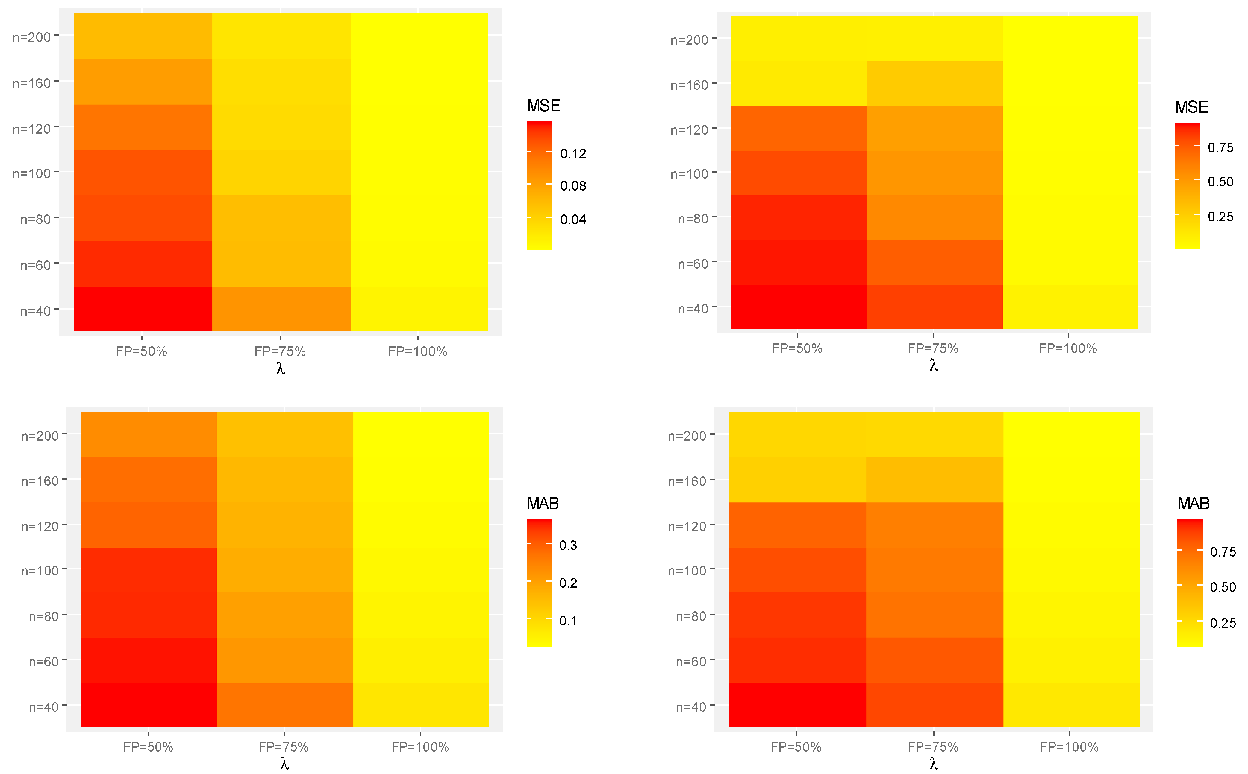
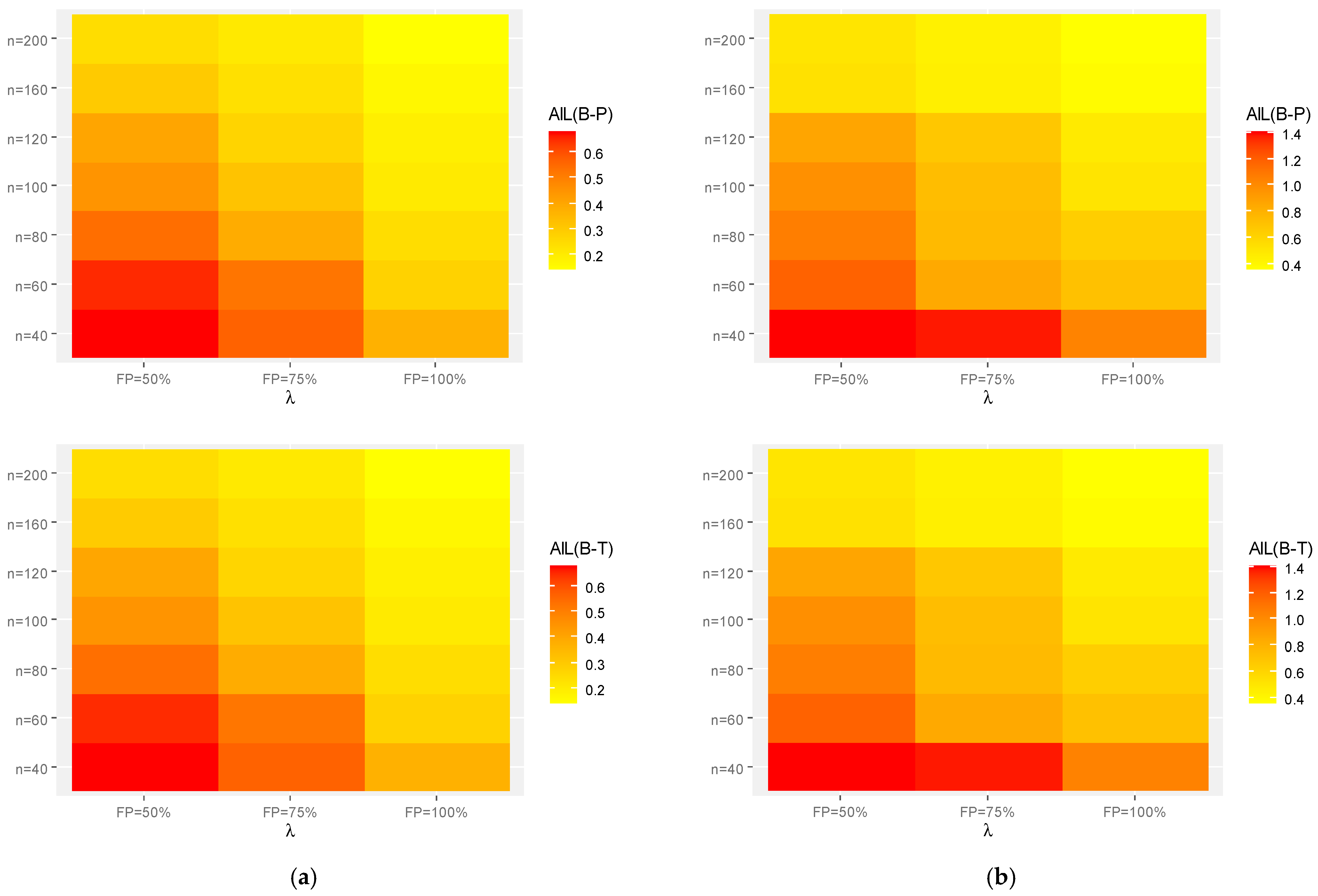
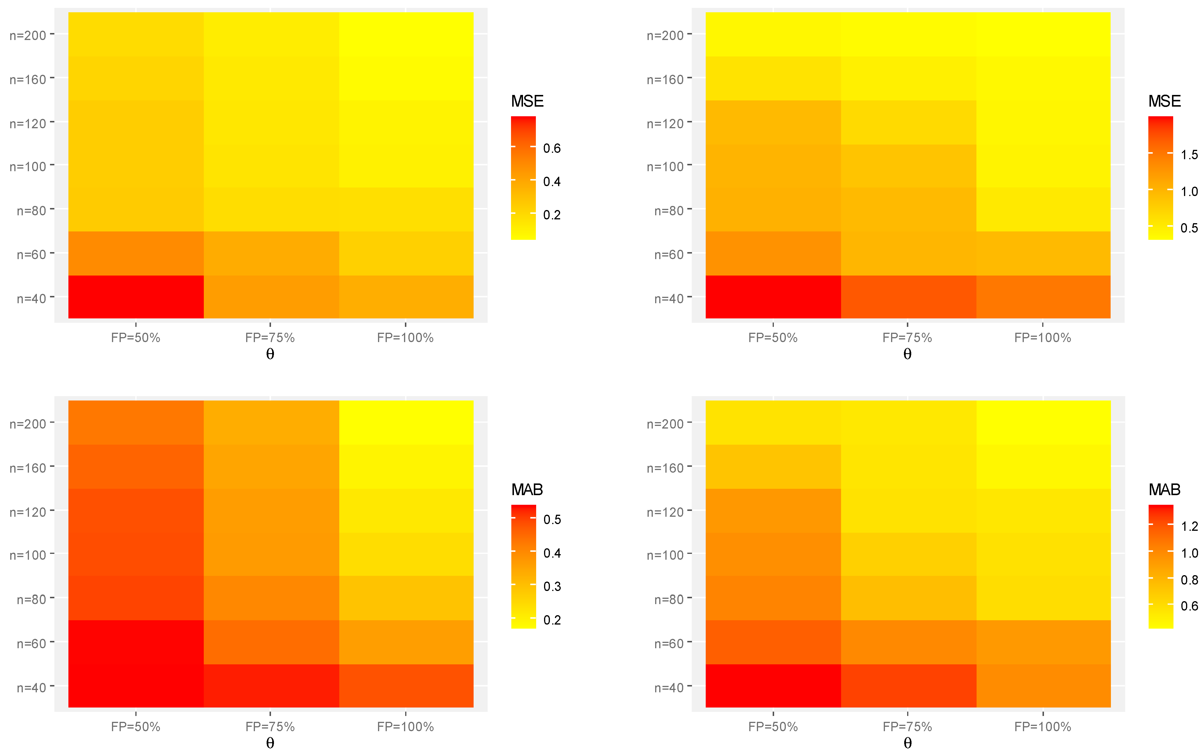
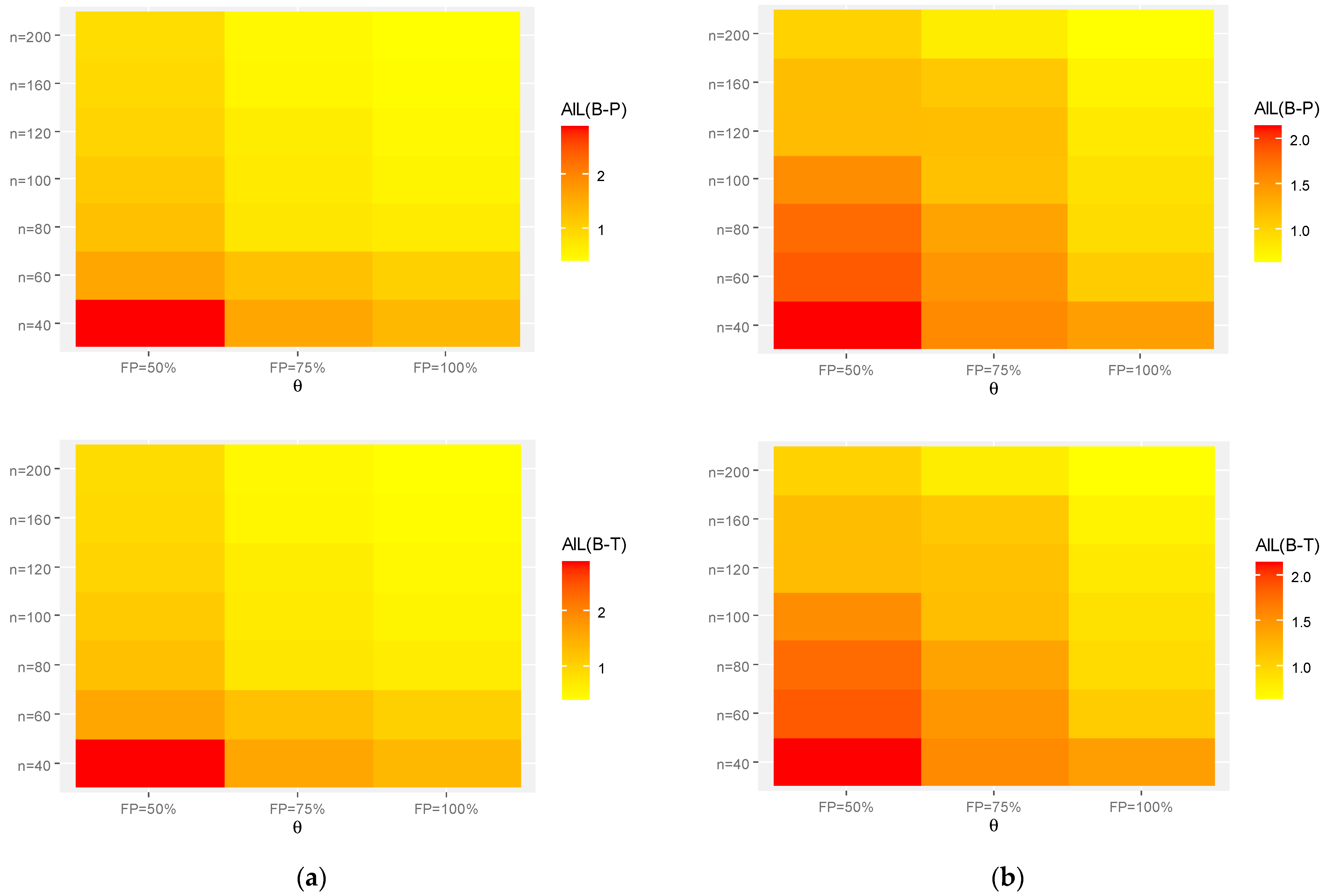
• Generally, in terms of lowest MSE, MAB, and AIL values, the acquired estimates of the unknown parameters $\beta ,\lambda ,$ and $\theta$ behave well;
• As $n$ increases, the MSEs, MABs, and AILs of $\beta ,\lambda ,$ and $\theta$ tend to decrease. This finding confirms the consistency feature of the associated estimates when the required sample size is increased. A similar pattern is observed when the FP increases;
• For fixed $(n,r)$, the interval estimates obtained from the B-T procedure have shorter AILs compared to those obtained from the B-P procedure. This result holds for all given parametric sets;
• As the true values of $\beta ,\lambda ,$ and $\theta$ increase, for each setting, the MSEs, MABs, and AILs of all unknown parameters $\beta ,\lambda ,$ or $\theta$ increase;
• As the true values of $\beta$ and $\theta$ increase, with fixing $\lambda$, the MSEs, MABs, and AILs of $\beta$ increase while those of $\lambda$ and $\theta$ decrease;
• In summary, the simulated results showed that the suggested estimation approaches of the DEC parameters perform well under Type-II censoring and can be easily extended to other models or other censoring plans;
• Heat-map visualization is a way of graphically representing numerical data where the value of each data point is indicated using specified colors. Therefore, utilizing the heat-map tool in R 4.2.2 programming software, the calculated point (or interval) estimates of $\beta ,\lambda ,$ or $\theta$ using Set-1 and Set-2 (for instant) are shown in Figure 3, Figure 4 and Figure 5, respectively.

Table 2. The AEs, MSEs, MABs, and AILs of $\beta$.

$\mathit{n}$	FP%	AE	MSE	MAB	AIL		AE	MSE	MAB	AIL		AE	MSE	MAB	AIL
					B-P	B-T				B-P	B-T				B-P	B-T
$\mathbf{Set}\to$		1					2					3
40	50%	0.0417	0.0220	0.0885	0.4530	0.4527	0.0829	0.0491	0.1756	0.8866	0.8871	1.7423	0.1920	0.3297	2.1419	2.1215
	75%	0.0519	0.0114	0.0844	0.2765	0.2759	0.1305	0.0332	0.1631	0.6168	0.6150	1.8229	0.1769	0.3237	1.8440	1.8268
	100%	0.1170	0.0102	0.0804	0.2410	0.2403	0.2375	0.0328	0.1460	0.4851	0.4855	1.4441	0.1581	0.3123	1.8148	1.7971
60	50%	0.0334	0.0124	0.0866	0.3711	0.3709	0.0338	0.0359	0.1720	0.6580	0.6581	1.7792	0.1479	0.3200	1.7803	1.7630
	75%	0.0332	0.0108	0.0807	0.2521	0.2518	0.2279	0.0316	0.1601	0.5594	0.5594	1.8179	0.1186	0.3195	1.7714	1.7544
	100%	0.1111	0.0078	0.0690	0.1939	0.1932	0.2573	0.0281	0.1294	0.2557	0.2560	1.5037	0.1099	0.3174	1.1769	1.1656
80	50%	0.0233	0.0075	0.0826	0.3046	0.3039	0.0264	0.0336	0.1696	0.6059	0.6060	1.6507	0.1094	0.3123	0.9369	0.9258
	75%	0.0305	0.0065	0.0741	0.1358	0.1347	0.2162	0.0309	0.1423	0.4935	0.4935	1.7861	0.1066	0.2916	0.9212	0.9123
	100%	0.1059	0.0062	0.0583	0.1245	0.1236	0.2737	0.0231	0.1105	0.2343	0.2342	1.4140	0.1048	0.2889	0.8439	0.8358
100	50%	0.0206	0.0072	0.0824	0.2543	0.2536	0.0453	0.0302	0.1625	0.5522	0.5522	1.8057	0.1033	0.2804	0.7529	0.7457
	75%	0.0332	0.0057	0.0711	0.1187	0.1181	0.1628	0.0276	0.1258	0.4919	0.4914	1.8167	0.1036	0.2779	0.7412	0.7341
	100%	0.1035	0.0043	0.0494	0.1034	0.1027	0.2117	0.0161	0.0928	0.2059	0.2058	1.4683	0.1023	0.2762	0.7269	0.7199
120	50%	0.0187	0.0071	0.0820	0.2394	0.2386	0.0334	0.0285	0.1471	0.5105	0.5101	1.7668	0.0995	0.2702	0.6836	0.6771
	75%	0.0343	0.0055	0.0709	0.1159	0.1150	0.2471	0.0170	0.1079	0.4469	0.4469	1.6029	0.0926	0.2488	0.6691	0.6626
	100%	0.1036	0.0038	0.0447	0.0878	0.0870	0.2139	0.0135	0.0861	0.1819	0.1818	1.4003	0.0916	0.2419	0.6045	0.5987
160	50%	0.0187	0.0069	0.0814	0.2113	0.2104	0.1077	0.0125	0.1016	0.3692	0.3693	1.7500	0.0871	0.2247	0.6001	0.5943
	75%	0.0300	0.0053	0.0688	0.0870	0.0863	0.1284	0.0123	0.0978	0.2833	0.2830	1.5132	0.0858	0.2244	0.5299	0.5248
	100%	0.1030	0.0027	0.0393	0.0662	0.0657	0.2101	0.0099	0.0747	0.1782	0.1781	1.3620	0.0689	0.2076	0.3221	0.3190
200	50%	0.0210	0.0065	0.0791	0.1720	0.1712	0.1036	0.0116	0.1008	0.3404	0.3403	1.6654	0.0571	0.1801	0.2432	0.2409
	75%	0.0335	0.0049	0.0672	0.0877	0.0866	0.1072	0.0117	0.0964	0.2133	0.2133	1.5955	0.0457	0.1630	0.2234	0.2213
	100%	0.1023	0.0021	0.0358	0.0667	0.0655	0.2086	0.0078	0.0687	0.1032	0.1032	1.2793	0.0398	0.1586	0.2155	0.2118

Table 2. The AEs, MSEs, MABs, and AILs of $\beta$.

$\mathit{n}$	FP%	AE	MSE	MAB	AIL		AE	MSE	MAB	AIL		AE	MSE	MAB	AIL
					B-P	B-T				B-P	B-T				B-P	B-T
$\mathbf{Set}\to$		1					2					3
40	50%	0.0417	0.0220	0.0885	0.4530	0.4527	0.0829	0.0491	0.1756	0.8866	0.8871	1.7423	0.1920	0.3297	2.1419	2.1215
	75%	0.0519	0.0114	0.0844	0.2765	0.2759	0.1305	0.0332	0.1631	0.6168	0.6150	1.8229	0.1769	0.3237	1.8440	1.8268
	100%	0.1170	0.0102	0.0804	0.2410	0.2403	0.2375	0.0328	0.1460	0.4851	0.4855	1.4441	0.1581	0.3123	1.8148	1.7971
60	50%	0.0334	0.0124	0.0866	0.3711	0.3709	0.0338	0.0359	0.1720	0.6580	0.6581	1.7792	0.1479	0.3200	1.7803	1.7630
	75%	0.0332	0.0108	0.0807	0.2521	0.2518	0.2279	0.0316	0.1601	0.5594	0.5594	1.8179	0.1186	0.3195	1.7714	1.7544
	100%	0.1111	0.0078	0.0690	0.1939	0.1932	0.2573	0.0281	0.1294	0.2557	0.2560	1.5037	0.1099	0.3174	1.1769	1.1656
80	50%	0.0233	0.0075	0.0826	0.3046	0.3039	0.0264	0.0336	0.1696	0.6059	0.6060	1.6507	0.1094	0.3123	0.9369	0.9258
	75%	0.0305	0.0065	0.0741	0.1358	0.1347	0.2162	0.0309	0.1423	0.4935	0.4935	1.7861	0.1066	0.2916	0.9212	0.9123
	100%	0.1059	0.0062	0.0583	0.1245	0.1236	0.2737	0.0231	0.1105	0.2343	0.2342	1.4140	0.1048	0.2889	0.8439	0.8358
100	50%	0.0206	0.0072	0.0824	0.2543	0.2536	0.0453	0.0302	0.1625	0.5522	0.5522	1.8057	0.1033	0.2804	0.7529	0.7457
	75%	0.0332	0.0057	0.0711	0.1187	0.1181	0.1628	0.0276	0.1258	0.4919	0.4914	1.8167	0.1036	0.2779	0.7412	0.7341
	100%	0.1035	0.0043	0.0494	0.1034	0.1027	0.2117	0.0161	0.0928	0.2059	0.2058	1.4683	0.1023	0.2762	0.7269	0.7199
120	50%	0.0187	0.0071	0.0820	0.2394	0.2386	0.0334	0.0285	0.1471	0.5105	0.5101	1.7668	0.0995	0.2702	0.6836	0.6771
	75%	0.0343	0.0055	0.0709	0.1159	0.1150	0.2471	0.0170	0.1079	0.4469	0.4469	1.6029	0.0926	0.2488	0.6691	0.6626
	100%	0.1036	0.0038	0.0447	0.0878	0.0870	0.2139	0.0135	0.0861	0.1819	0.1818	1.4003	0.0916	0.2419	0.6045	0.5987
160	50%	0.0187	0.0069	0.0814	0.2113	0.2104	0.1077	0.0125	0.1016	0.3692	0.3693	1.7500	0.0871	0.2247	0.6001	0.5943
	75%	0.0300	0.0053	0.0688	0.0870	0.0863	0.1284	0.0123	0.0978	0.2833	0.2830	1.5132	0.0858	0.2244	0.5299	0.5248
	100%	0.1030	0.0027	0.0393	0.0662	0.0657	0.2101	0.0099	0.0747	0.1782	0.1781	1.3620	0.0689	0.2076	0.3221	0.3190
200	50%	0.0210	0.0065	0.0791	0.1720	0.1712	0.1036	0.0116	0.1008	0.3404	0.3403	1.6654	0.0571	0.1801	0.2432	0.2409
	75%	0.0335	0.0049	0.0672	0.0877	0.0866	0.1072	0.0117	0.0964	0.2133	0.2133	1.5955	0.0457	0.1630	0.2234	0.2213
	100%	0.1023	0.0021	0.0358	0.0667	0.0655	0.2086	0.0078	0.0687	0.1032	0.1032	1.2793	0.0398	0.1586	0.2155	0.2118

Table 3. The AEs, MSEs, MABs and AILs of $\lambda$ .

$\mathit{n}$	FP%	AE	MSE	MAB	AIL		AE	MSE	MAB	AIL		AE	MSE	MAB	AIL
					B-P	B-T				B-P	B-T				B-P	B-T
$\mathbf{Set}\to$		1					2					3
40	50%	0.6916	0.1583	0.3686	0.6839	0.6822	1.2733	0.9213	0.9825	1.4147	1.4139	0.9221	0.4349	0.6402	0.7928	0.7843
	75%	0.5987	0.0911	0.2722	0.5699	0.5687	1.1841	0.8264	0.8706	1.3871	1.3868	0.8505	0.4316	0.6520	0.7792	0.7714
	100%	0.4360	0.0107	0.0777	0.3745	0.3739	0.8824	0.0737	0.1925	1.0514	1.0510	1.1350	0.4045	0.6197	0.7683	0.7606
60	50%	0.8681	0.1498	0.3620	0.6559	0.6523	1.0706	0.9001	0.9280	1.1927	1.1919	0.9990	0.3856	0.6141	0.7507	0.7439
	75%	0.6710	0.0595	0.2186	0.5292	0.5272	0.9084	0.7432	0.8218	0.8597	0.8591	0.8594	0.3798	0.5888	0.7309	0.7236
	100%	0.4214	0.0058	0.0594	0.2807	0.2786	0.8423	0.0345	0.1402	0.7242	0.7235	1.1592	0.3641	0.5350	0.7156	0.7113
80	50%	0.7619	0.1366	0.3508	0.5429	0.5408	1.7280	0.8804	0.9094	1.0749	1.0744	1.0939	0.3567	0.5592	0.7058	0.7016
	75%	0.6183	0.0572	0.2032	0.3915	0.3896	1.6218	0.5785	0.7292	0.7637	0.7636	0.8831	0.3332	0.5422	0.6987	0.6949
	100%	0.4173	0.0042	0.0504	0.2478	0.2469	0.8373	0.0277	0.1222	0.6500	0.6492	1.1489	0.3181	0.5504	0.6786	0.6746
100	50%	0.7508	0.1325	0.3491	0.4523	0.4513	1.5840	0.7995	0.8509	0.9872	0.9869	0.8966	0.2587	0.4511	0.6773	0.6732
	75%	0.5818	0.0393	0.1822	0.3231	0.3217	1.5030	0.5212	0.7030	0.7459	0.7450	0.9098	0.2085	0.3748	0.6305	0.6267
	100%	0.4132	0.0030	0.0427	0.2100	0.2089	0.8259	0.0176	0.1016	0.5257	0.5248	1.4402	0.1662	0.2939	0.6273	0.6235
120	50%	0.7491	0.1135	0.2941	0.4066	0.4051	1.5624	0.7154	0.7849	0.8834	0.8825	0.9474	0.1385	0.2633	0.6249	0.6212
	75%	0.5622	0.0336	0.1730	0.2741	0.2721	1.5292	0.4800	0.6831	0.6931	0.6923	1.1251	0.1064	0.1990	0.5931	0.5908
	100%	0.4103	0.0024	0.0378	0.1943	0.1933	0.8171	0.0142	0.0922	0.4907	0.4902	1.1420	0.0982	0.1774	0.5867	0.5844
160	50%	0.6805	0.0844	0.2805	0.3025	0.3013	1.4831	0.1178	0.3103	0.5457	0.5450	1.0633	0.0818	0.1521	0.5630	0.5608
	75%	0.5730	0.0311	0.1625	0.2398	0.2387	1.0662	0.2725	0.4039	0.4601	0.4593	1.1342	0.0672	0.1398	0.4719	0.4680
	100%	0.4074	0.0018	0.0324	0.1689	0.1679	0.8127	0.0102	0.0792	0.3860	0.3849	1.0414	0.0631	0.1266	0.3059	0.3047
200	50%	0.6367	0.0599	0.2367	0.2491	0.2483	1.1102	0.0882	0.2767	0.5193	0.5184	1.0748	0.0599	0.1131	0.2783	0.2769
	75%	0.5482	0.0246	0.1482	0.2142	0.2132	1.0655	0.0839	0.2656	0.4474	0.4465	1.1350	0.0391	0.0894	0.2674	0.2670
	100%	0.4059	0.0014	0.0298	0.1452	0.1446	0.8100	0.0085	0.0723	0.3647	0.3639	1.0520	0.0337	0.0805	0.2587	0.2485

Table 3. The AEs, MSEs, MABs and AILs of $\lambda$ .

$\mathit{n}$	FP%	AE	MSE	MAB	AIL		AE	MSE	MAB	AIL		AE	MSE	MAB	AIL
					B-P	B-T				B-P	B-T				B-P	B-T
$\mathbf{Set}\to$		1					2					3
40	50%	0.6916	0.1583	0.3686	0.6839	0.6822	1.2733	0.9213	0.9825	1.4147	1.4139	0.9221	0.4349	0.6402	0.7928	0.7843
	75%	0.5987	0.0911	0.2722	0.5699	0.5687	1.1841	0.8264	0.8706	1.3871	1.3868	0.8505	0.4316	0.6520	0.7792	0.7714
	100%	0.4360	0.0107	0.0777	0.3745	0.3739	0.8824	0.0737	0.1925	1.0514	1.0510	1.1350	0.4045	0.6197	0.7683	0.7606
60	50%	0.8681	0.1498	0.3620	0.6559	0.6523	1.0706	0.9001	0.9280	1.1927	1.1919	0.9990	0.3856	0.6141	0.7507	0.7439
	75%	0.6710	0.0595	0.2186	0.5292	0.5272	0.9084	0.7432	0.8218	0.8597	0.8591	0.8594	0.3798	0.5888	0.7309	0.7236
	100%	0.4214	0.0058	0.0594	0.2807	0.2786	0.8423	0.0345	0.1402	0.7242	0.7235	1.1592	0.3641	0.5350	0.7156	0.7113
80	50%	0.7619	0.1366	0.3508	0.5429	0.5408	1.7280	0.8804	0.9094	1.0749	1.0744	1.0939	0.3567	0.5592	0.7058	0.7016
	75%	0.6183	0.0572	0.2032	0.3915	0.3896	1.6218	0.5785	0.7292	0.7637	0.7636	0.8831	0.3332	0.5422	0.6987	0.6949
	100%	0.4173	0.0042	0.0504	0.2478	0.2469	0.8373	0.0277	0.1222	0.6500	0.6492	1.1489	0.3181	0.5504	0.6786	0.6746
100	50%	0.7508	0.1325	0.3491	0.4523	0.4513	1.5840	0.7995	0.8509	0.9872	0.9869	0.8966	0.2587	0.4511	0.6773	0.6732
	75%	0.5818	0.0393	0.1822	0.3231	0.3217	1.5030	0.5212	0.7030	0.7459	0.7450	0.9098	0.2085	0.3748	0.6305	0.6267
	100%	0.4132	0.0030	0.0427	0.2100	0.2089	0.8259	0.0176	0.1016	0.5257	0.5248	1.4402	0.1662	0.2939	0.6273	0.6235
120	50%	0.7491	0.1135	0.2941	0.4066	0.4051	1.5624	0.7154	0.7849	0.8834	0.8825	0.9474	0.1385	0.2633	0.6249	0.6212
	75%	0.5622	0.0336	0.1730	0.2741	0.2721	1.5292	0.4800	0.6831	0.6931	0.6923	1.1251	0.1064	0.1990	0.5931	0.5908
	100%	0.4103	0.0024	0.0378	0.1943	0.1933	0.8171	0.0142	0.0922	0.4907	0.4902	1.1420	0.0982	0.1774	0.5867	0.5844
160	50%	0.6805	0.0844	0.2805	0.3025	0.3013	1.4831	0.1178	0.3103	0.5457	0.5450	1.0633	0.0818	0.1521	0.5630	0.5608
	75%	0.5730	0.0311	0.1625	0.2398	0.2387	1.0662	0.2725	0.4039	0.4601	0.4593	1.1342	0.0672	0.1398	0.4719	0.4680
	100%	0.4074	0.0018	0.0324	0.1689	0.1679	0.8127	0.0102	0.0792	0.3860	0.3849	1.0414	0.0631	0.1266	0.3059	0.3047
200	50%	0.6367	0.0599	0.2367	0.2491	0.2483	1.1102	0.0882	0.2767	0.5193	0.5184	1.0748	0.0599	0.1131	0.2783	0.2769
	75%	0.5482	0.0246	0.1482	0.2142	0.2132	1.0655	0.0839	0.2656	0.4474	0.4465	1.1350	0.0391	0.0894	0.2674	0.2670
	100%	0.4059	0.0014	0.0298	0.1452	0.1446	0.8100	0.0085	0.0723	0.3647	0.3639	1.0520	0.0337	0.0805	0.2587	0.2485

Table 4. The AEs, MSEs, MABs and AILs of $\theta$.

$\mathit{n}$	FP%	AE	MSE	MAB	AIL		AE	MSE	MAB	AIL		AE	MSE	MAB	AIL
					B-P	B-T				B-P	B-T				B-P	B-T
$\mathbf{Set}\to$		1					2					3
40	50%	0.4446	0.7854	0.5406	2.1597	2.1594	0.9829	1.9999	1.3528	2.9249	2.9226	0.3798	0.1594	0.3986	1.1072	1.1050
	75%	0.5394	0.4391	0.5289	1.5823	1.5810	1.1107	1.7040	1.2528	1.6133	1.6130	0.3754	0.1570	0.3943	0.9912	0.9894
	100%	0.9934	0.3775	0.4820	1.3819	1.3825	1.3396	1.5040	0.9932	1.4323	1.4312	0.3255	0.1566	0.3950	0.9883	0.9861
60	50%	0.3305	0.5004	0.5388	1.6101	1.6099	0.9910	1.2992	1.1668	1.8858	1.8847	0.3193	0.1479	0.3774	0.9484	0.9465
	75%	0.4060	0.3853	0.4465	1.2698	1.2684	1.1738	1.0025	1.0051	1.4980	1.4953	0.3629	0.1470	0.3787	0.8063	0.8047
	100%	0.8813	0.2431	0.3643	1.0588	1.0574	1.2706	0.9674	0.9329	1.0675	1.0641	0.3708	0.1428	0.3692	0.7308	0.7294
80	50%	0.3257	0.2618	0.4983	1.2735	1.2751	1.2389	1.0495	1.0245	1.7836	1.7829	0.3325	0.1407	0.3636	0.7157	0.7143
	75%	0.4199	0.1895	0.4029	0.7621	0.7620	1.4924	0.9604	0.7603	1.3942	1.3937	0.3503	0.1200	0.3245	0.6947	0.6946
	100%	0.8424	0.1843	0.2925	0.6855	0.6846	1.7427	0.5398	0.6040	0.9418	0.9408	0.3236	0.1189	0.3078	0.6603	0.6594
100	50%	0.3196	0.2543	0.4888	1.1413	1.1415	1.2652	1.0176	0.9790	1.5616	1.5607	0.3561	0.1176	0.3304	0.6305	0.6293
	75%	0.4480	0.1611	0.3699	0.7046	0.7042	1.5613	0.8758	0.6701	1.1564	1.1816	0.3433	0.0949	0.2598	0.6161	0.6147
	100%	0.8245	0.1085	0.2414	0.5535	0.5531	1.6614	0.4450	0.5824	0.8965	0.8943	0.3984	0.0914	0.2803	0.5596	0.5586
120	50%	0.3128	0.2535	0.4856	1.0088	1.0091	1.3561	0.9651	0.9370	1.2006	1.2010	0.3829	0.0835	0.1706	0.5497	0.5486
	75%	0.4620	0.1494	0.3649	0.6646	0.6652	1.3951	0.6821	0.5789	1.1810	1.1549	0.3223	0.0789	0.2288	0.5155	0.5136
	100%	0.8224	0.0964	0.2203	0.5034	0.5032	1.6541	0.4144	0.5547	0.8301	0.8286	0.3311	0.0574	0.1939	0.3822	0.3810
160	50%	0.3416	0.2223	0.4587	0.9346	0.9347	1.4312	0.5939	0.7273	1.1889	1.1872	0.3468	0.0548	0.1682	0.3634	0.3627
	75%	0.4386	0.1441	0.3520	0.5255	0.5256	1.4874	0.4699	0.5650	1.1013	1.1002	0.3809	0.0533	0.1782	0.3481	0.3483
	100%	0.8160	0.0659	0.1937	0.4364	0.4362	1.6094	0.3943	0.4697	0.7415	0.7402	0.3332	0.0504	0.1771	0.3123	0.3117
200	50%	0.3708	0.1953	0.4294	0.8913	0.8920	1.5361	0.4075	0.5755	1.0186	1.0190	0.3591	0.0464	0.1477	0.3079	0.3073
	75%	0.4655	0.1280	0.3373	0.4937	0.4941	1.5888	0.3691	0.5464	0.7932	0.7932	0.3173	0.0375	0.1397	0.2965	0.2947
	100%	0.8125	0.0497	0.1707	0.3997	0.4001	1.6509	0.3306	0.4265	0.6376	0.6359	0.3022	0.0357	0.1282	0.2901	0.2884

Table 4. The AEs, MSEs, MABs and AILs of $\theta$.

$\mathit{n}$	FP%	AE	MSE	MAB	AIL		AE	MSE	MAB	AIL		AE	MSE	MAB	AIL
					B-P	B-T				B-P	B-T				B-P	B-T
$\mathbf{Set}\to$		1					2					3
40	50%	0.4446	0.7854	0.5406	2.1597	2.1594	0.9829	1.9999	1.3528	2.9249	2.9226	0.3798	0.1594	0.3986	1.1072	1.1050
	75%	0.5394	0.4391	0.5289	1.5823	1.5810	1.1107	1.7040	1.2528	1.6133	1.6130	0.3754	0.1570	0.3943	0.9912	0.9894
	100%	0.9934	0.3775	0.4820	1.3819	1.3825	1.3396	1.5040	0.9932	1.4323	1.4312	0.3255	0.1566	0.3950	0.9883	0.9861
60	50%	0.3305	0.5004	0.5388	1.6101	1.6099	0.9910	1.2992	1.1668	1.8858	1.8847	0.3193	0.1479	0.3774	0.9484	0.9465
	75%	0.4060	0.3853	0.4465	1.2698	1.2684	1.1738	1.0025	1.0051	1.4980	1.4953	0.3629	0.1470	0.3787	0.8063	0.8047
	100%	0.8813	0.2431	0.3643	1.0588	1.0574	1.2706	0.9674	0.9329	1.0675	1.0641	0.3708	0.1428	0.3692	0.7308	0.7294
80	50%	0.3257	0.2618	0.4983	1.2735	1.2751	1.2389	1.0495	1.0245	1.7836	1.7829	0.3325	0.1407	0.3636	0.7157	0.7143
	75%	0.4199	0.1895	0.4029	0.7621	0.7620	1.4924	0.9604	0.7603	1.3942	1.3937	0.3503	0.1200	0.3245	0.6947	0.6946
	100%	0.8424	0.1843	0.2925	0.6855	0.6846	1.7427	0.5398	0.6040	0.9418	0.9408	0.3236	0.1189	0.3078	0.6603	0.6594
100	50%	0.3196	0.2543	0.4888	1.1413	1.1415	1.2652	1.0176	0.9790	1.5616	1.5607	0.3561	0.1176	0.3304	0.6305	0.6293
	75%	0.4480	0.1611	0.3699	0.7046	0.7042	1.5613	0.8758	0.6701	1.1564	1.1816	0.3433	0.0949	0.2598	0.6161	0.6147
	100%	0.8245	0.1085	0.2414	0.5535	0.5531	1.6614	0.4450	0.5824	0.8965	0.8943	0.3984	0.0914	0.2803	0.5596	0.5586
120	50%	0.3128	0.2535	0.4856	1.0088	1.0091	1.3561	0.9651	0.9370	1.2006	1.2010	0.3829	0.0835	0.1706	0.5497	0.5486
	75%	0.4620	0.1494	0.3649	0.6646	0.6652	1.3951	0.6821	0.5789	1.1810	1.1549	0.3223	0.0789	0.2288	0.5155	0.5136
	100%	0.8224	0.0964	0.2203	0.5034	0.5032	1.6541	0.4144	0.5547	0.8301	0.8286	0.3311	0.0574	0.1939	0.3822	0.3810
160	50%	0.3416	0.2223	0.4587	0.9346	0.9347	1.4312	0.5939	0.7273	1.1889	1.1872	0.3468	0.0548	0.1682	0.3634	0.3627
	75%	0.4386	0.1441	0.3520	0.5255	0.5256	1.4874	0.4699	0.5650	1.1013	1.1002	0.3809	0.0533	0.1782	0.3481	0.3483
	100%	0.8160	0.0659	0.1937	0.4364	0.4362	1.6094	0.3943	0.4697	0.7415	0.7402	0.3332	0.0504	0.1771	0.3123	0.3117
200	50%	0.3708	0.1953	0.4294	0.8913	0.8920	1.5361	0.4075	0.5755	1.0186	1.0190	0.3591	0.0464	0.1477	0.3079	0.3073
	75%	0.4655	0.1280	0.3373	0.4937	0.4941	1.5888	0.3691	0.5464	0.7932	0.7932	0.3173	0.0375	0.1397	0.2965	0.2947
	100%	0.8125	0.0497	0.1707	0.3997	0.4001	1.6509	0.3306	0.4265	0.6376	0.6359	0.3022	0.0357	0.1282	0.2901	0.2884

Figure 3. Heat-maps for the Monte Carlo results of $\beta$. (a) Set-1. (b) Set-2.

Figure 3. Heat-maps for the Monte Carlo results of $\beta$. (a) Set-1. (b) Set-2.

Figure 4. Heat-maps for the Monte Carlo results of $\lambda$. (a) Set-1. (b) Set-2.

Figure 4. Heat-maps for the Monte Carlo results of $\lambda$. (a) Set-1. (b) Set-2.

Figure 5. Heat-maps for the Monte Carlo results of $\theta$. (a) Set-1. (b) Set-2.

Figure 5. Heat-maps for the Monte Carlo results of $\theta$. (a) Set-1. (b) Set-2.

4. Real-Life Applications

This section presents the analysis of two applications utilizing different real data sets in order to (i) examine the usefulness and adaptability of the offered model to real phenomena; (ii) demonstrate the applicability of the inferential results to a real practical situation; and (iii) evaluate to see whether the proposed model is a better choice than the other eleven models. The first application examines the number of vehicle fatalities for thirty-nine counties in the state of South Carolina in 2012, acquired from the National Highway Traffic Safety Administration’s (www-fars.nhtsa.dot.gov, accessed on 13 January 2023). Firstly, this data set (denoted by Data-I) was reported by ref. [42]. Another application provides an analysis of the final exam marks in 2004 of 48 slow-paced students in mathematics at the Indian Institute of Technology at Kanpur. This data set (denoted by Data-II) is taken from ref. [43] and reanalyzed by ref. [44]. It is better to point out here that the number of vehicle deaths or check marks have the same philosophy of separate data points as in different cases in nature, such as weights, heights, ages, etc. The data sets I and II are reported in

Table 5. Complete data sets I and II.

Data-I	22, 26, 17, 4, 48, 9, 9, 31, 27, 20, 12, 6, 5, 14, 9, 16, 3, 33, 9, 20, 68, 13, 51, 13, 2, 4,17, 16, 6, 52, 50, 48, 23, 12, 13, 10, 15, 8, 1
Data-II	29, 25, 50, 15, 13, 27, 15, 18, 7, 7, 8, 19, 12, 18, 5, 21, 15, 86, 21, 15, 14, 39, 15, 14, 70, 44, 6, 23, 58, 19, 50, 23, 11, 6, 34, 18, 28, 34, 12, 37, 4, 60, 20, 23, 40, 65, 19, 31

, while their statistics, namely: min, max, (first, second, and third) quartiles $Q_i,i=1,\mathrm{2,3}$, mode, mean, standard deviation (St.D), $Sk$, and Ku, are listed in

Table 6. Vital summary statistics of data sets I and II.

Data	Min	Max	${\mathit{Q}}_1$	${\mathit{Q}}_2$	${\mathit{Q}}_3$	Mode	Mean	St.D	Skew.	Kurt.
I	1	68	9	14	24.5	9	19.538	16.507	1.288	3.798
II	4	86	14	19.5	34	15	25.896	18.605	1.332	4.323

.

To demonstrate the validity and superiority of the proposed model, based on the first and second datasets, the DEC probability model is compared alongside the other eleven competing models in the literature, namely: Poisson (P$\left(\theta \right)$) by ref. [45], discrete Weibull (DW$(\lambda ,\theta )$) by ref. [44], negative binomial (NB$(n,\theta )$) and geometric (G$\left(p\right)$) discussed by ref. [46], discrete Burr Type XII (DB$(\lambda ,\theta$) by ref. [4], discrete generalized-exponential (DGE$(\lambda ,\theta )$) by ref. [47], discrete gamma (DG$(\lambda ,\theta )$) by ref. [6], discrete Burr Hatke (DBH$\left(\theta \right)$) by ref. [48], discrete Nadarajah-Haghighi (DNH$(\lambda ,\theta )$) by ref. [10], discrete modified Weibull (DMW$(\alpha ,\lambda ,\theta )$) by ref. [49], and exponentiated discrete Weibull (EDW$(\alpha ,\lambda ,\theta )$) by ref. [7] distributions.

To specify the best model, several criteria are used, namely: negative log-likelihood (NLL$=-\widehat{𝓁}$), Akaike ($\mathrm{A}=2\pi -2\widehat{𝓁}$), consistent Akaike ($\mathrm{C}\mathrm{A}=-2\widehat{𝓁}+2n\pi {\left(n-\pi -1\right)}^{-1}$), Bayesian ($\mathrm{B}=-2\widehat{𝓁}+\pi \mathrm{l}\mathrm{o}\mathrm{g}\left(n\right)$) and Hannan-Quinn (HQ$=-2\widehat{𝓁}+\pi \mathrm{l}\mathrm{o}\mathrm{g}(\mathrm{l}\mathrm{o}\mathrm{g}(n\left)\right)$) information criteria, where $\pi$ is the length of the model parameter vector. Besides them, the Kolmogorov-Smirnov (K-S) statistic with its $p$-value is also considered. Obviously, the best probability model distribution gives the best fit for a given set of data if it has the highest $p$-value and the lowest values of all other measures. Via R programming software 4.2.2, by installing the ‘AdequacyModel’ package proposed by ref. [50], the maximum likelihood estimates (with their standard errors (St.Es)) as well as the fitted model selection criteria are presented in

Table 7. Summary fit (St.E) of the DEC model and its competing models from data sets I and II.

Model	$\mathit{\alpha }$	$\mathit{\lambda }$	$\mathit{\theta }$	NLL	A	CA	B	H-Q	K-S ($\mathit{p}$-Value)
	Data-I
DEC	0.5207 (0.4120)	0.2215 (0.0599)	10.139 (11.773)	153.121	309.781	309.889	311.445	310.378	0.088 (0.920)
DMW	0.6727 (0.0947)	1.2965 (0.3646)	1.2965 (0.3646)	210.594	427.187	427.732	432.801	429.308	0.204 (0.036)
EDW	0.7930 (0.3019)	0.7278 (0.3622)	0.9389 (0.0518)	196.492	398.984	399.529	404.597	401.105	0.092 (0.914)
DGE	1.7338 (0.4101)	0.0695 (0.0130)	-	153.365	310.730	311.064	314.057	311.924	0.111 (0.721)
DNH	1.9281 (1.1305)	0.0200 (0.0155)	-	154.907	313.814	314.147	317.141	315.008	0.110 (0.730)
DB	14.531 (46.924)	0.0260 (0.0838)	-	214.879	431.758	431.866	433.421	432.354	0.758 (0.001)
DW	1.2974 (0.1582)	21.791 (2.8466)	-	180.934	365.868	366.201	369.195	367.062	0.338 (0.003)
DG	0.0816 (0.0198)	1.6343 (0.3401)	-	153.907	311.814	312.148	315.141	313.008	0.126 (0.570)
NB	19.534 (2.5126)	1.6827 (0.3936)	-	153.458	310.917	311.250	314.244	312.110	0.116 (0.667)
DBH	0.9985 (0.0064)	-	-	153.609	311.218	311.551	314.545	312.411	0.097 (0.854)
G	0.0487 (0.0076)	-	-	155.904	313.809	313.917	315.472	314.406	0.162 (0.257)
P	19.539 (0.7078)	-	-	324.089	650.178	650.286	651.841	650.775	0.407 (0.002)
	Data-II
DEC	0.6483 (0.5218)	0.2064 (0.0569)	25.021 (36.898)	196.448	397.903	398.170	400.984	399.317	0.080 (0.917)
DMW	0.9429 (0.0826)	0.8011 (1.7965)	1.0309 (0.0087)	153.699	309.939	310.085	314.390	311.190	0.135 (0.479)
EDW	0.7051 (0.3785)	0.6433 (0.3169)	8.0766 (11.453)	153.153	312.307	312.993	317.298	314.097	0.090 (0.912)
DGE	2.6662 (0.6283)	0.0657 (0.0102)	-	196.951	398.897	399.199	401.645	399.820	0.108 (0.632)
DNH	3.7619 (2.1185)	0.0070 (0.0046)	-	201.743	407.485	407.752	411.228	408.899	0.155 (0.201)
DB	4.7414 (13.418)	0.0693 (0.1964)	-	297.676	597.352	597.439	599.223	598.059	0.837 (0.001)
DW	1.5458 (0.1666)	29.549 (2.9245)	-	247.486	498.971	499.238	502.714	500.385	0.403 (0.002)
DG	0.0879 (0.0188)	2.3093 (0.4419)	-	198.609	401.217	401.484	404.960	402.631	0.132 (0.371)
NB	25.896 (2.5012)	2.4440 (0.5219)	-	197.296	398.593	398.860	402.335	400.007	0.115 (0.553)
DBH	0.9990 (0.0046)	-	-	197.522	399.044	399.310	402.786	400.458	0.095 (0.774)
G	0.0372 (0.0053)	-	-	205.111	412.222	412.309	414.093	412.929	0.222 (0.017)
P	25.896 (0.7345)	-	-	396.589	795.178	795.265	797.050	795.886	0.400 (0.004)

.

It is evident from the Data-I fit in Table 7 that the DEC distribution, which has the lowest statistical values and the highest $p$-value among all the fitted competitive models, is the best model. Also, from the Data-II fit in Table 7, it is clear that the DEC distribution, with respect to the $p$-value, is the best distribution among all compared models, while the other three-parameter DMW and EDW distributions perform better with respect to the other given criteria. 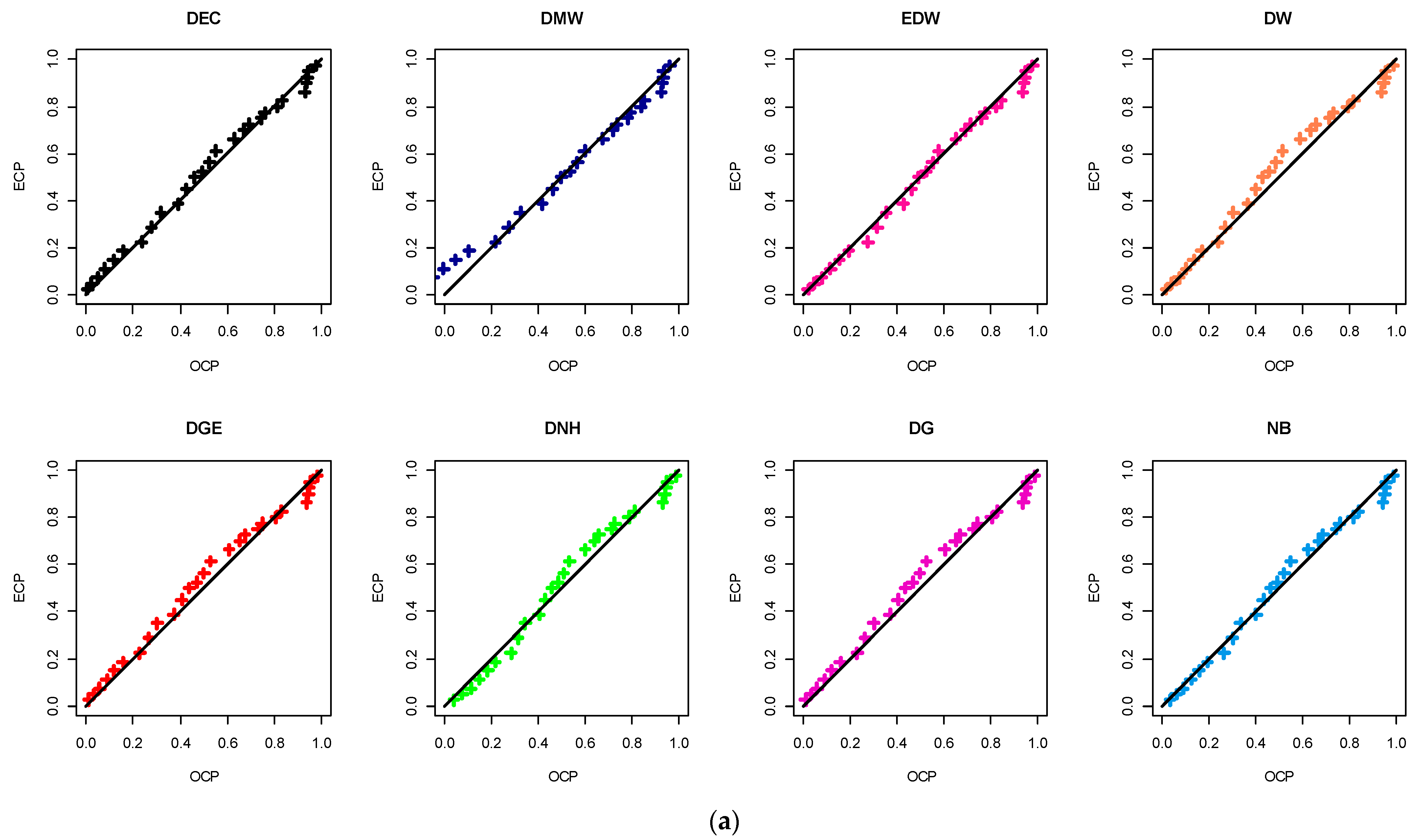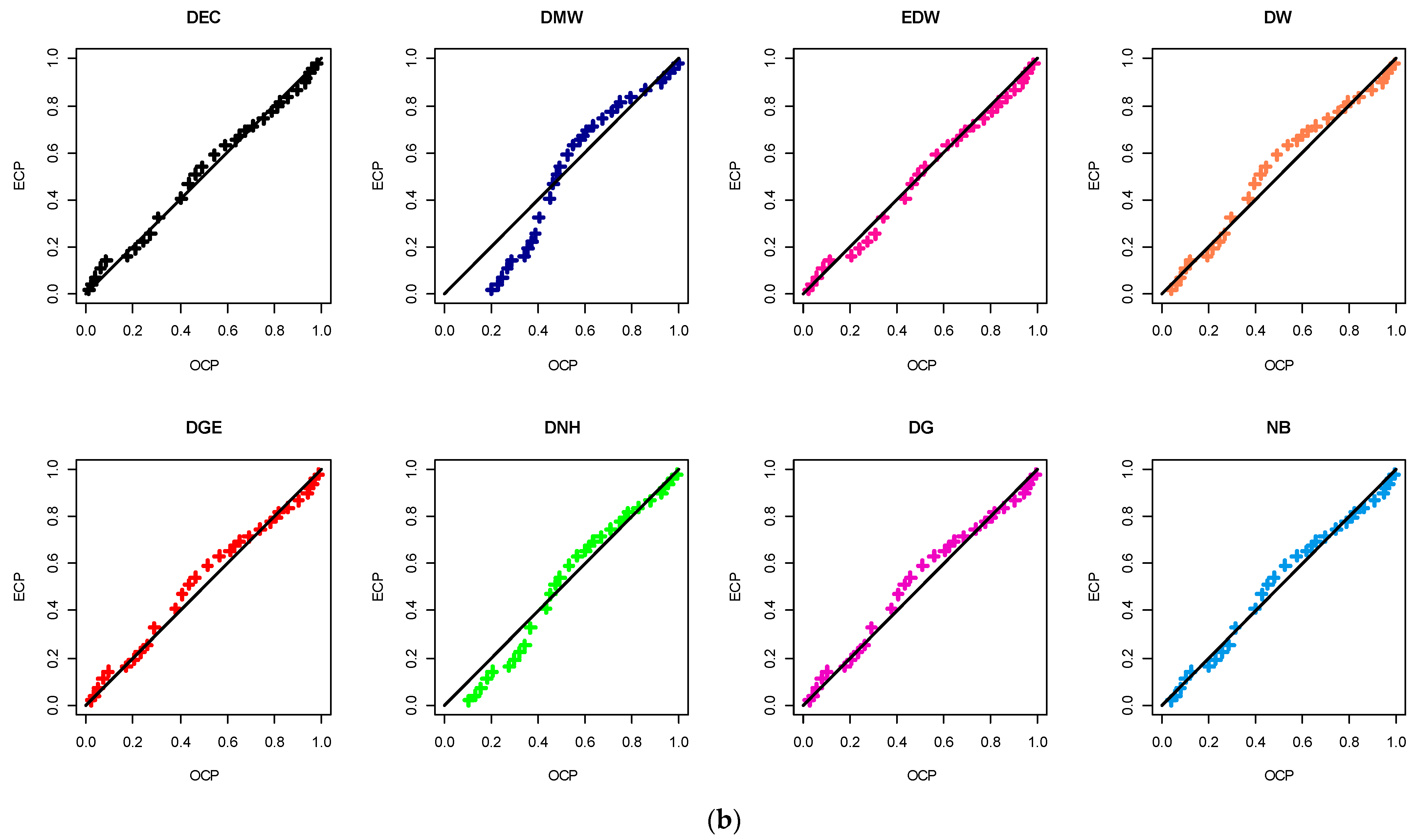Further, in Figure 6, the corresponding probability-probability (PP) plot is a visual plot showing the relationship between observed cumulative probability (OCP) and expected cumulative probability (ECP) of the DEC distribution and its competing distributions. 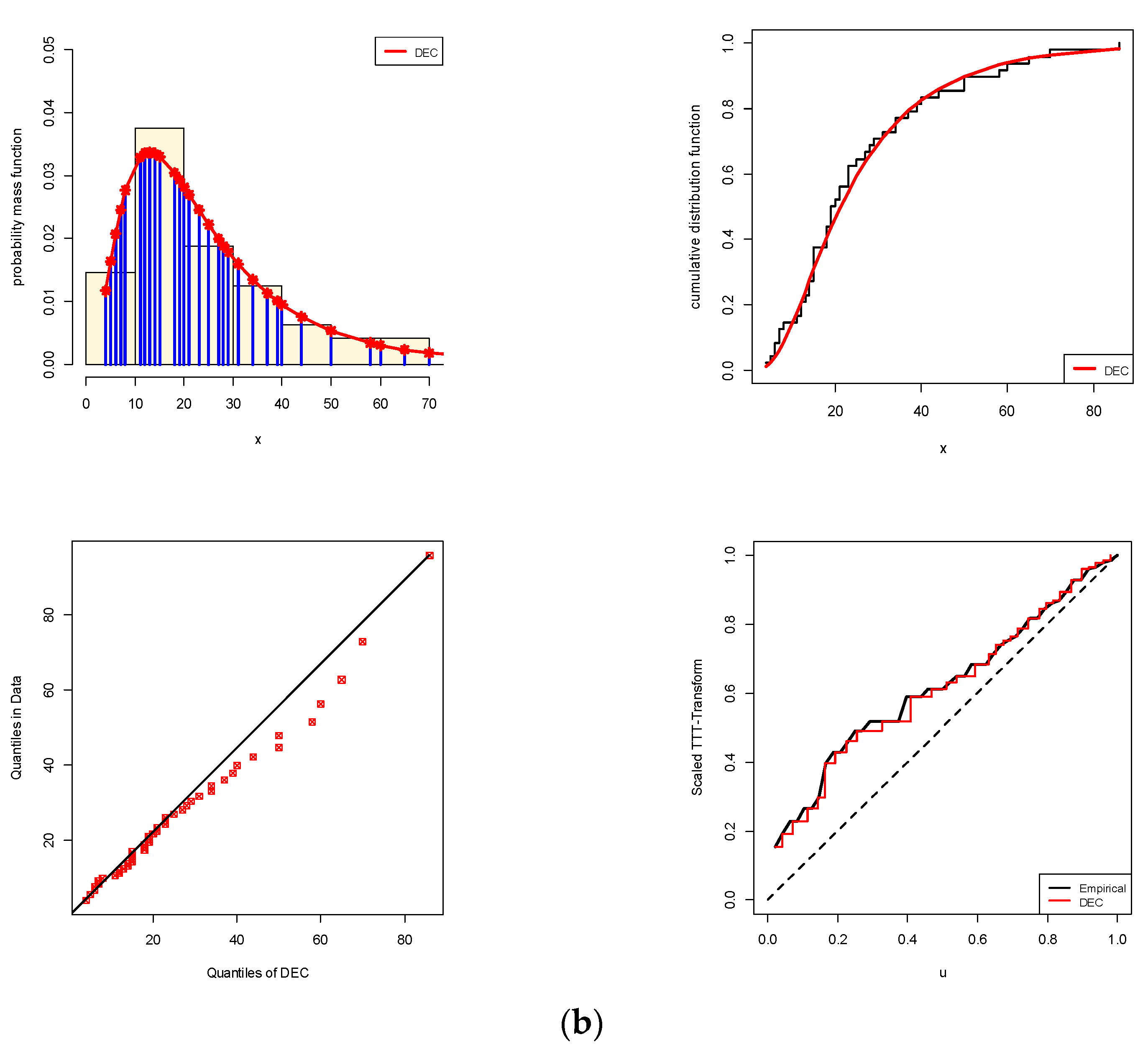It also supports our findings in Table 7. Various visualization goodness tools, namely (i) histogram with fitted PDF, (ii) fitted CDF, (iii) quantile-quantile (QQ), and (iv) total time test (TTT) plots, are utilized to show the goodness-of-fit of a theoretical model to observed data; see Figure 7. It is evident, from both data sets I and II, that (i) the fitted DEC density captures the general pattern of the histograms well; (ii) all estimated DEC distribution (or quantile) points are quite close to the straight line; and (iii) the DEC failure rate has an increasing shape. As a result, from the empirical results, we can conclude that the new DEC distribution provides a significantly good fit compared to the other traditional (or newly developed) discrete statistical models.

Now, to evaluate the acquired estimates of $\beta ,\lambda ,$ and $\theta$ developed by maximum likelihood and bootstrap (based on 10,000 replications) methods in a real scenario, three Type-II censored samples from each data set in Table 5 are generated based on different values of $r$; see

Table 8. Type-II censored samples from data sets I and II.

Data	Sample	$(\mathit{n},\mathit{r})$	Censored Data
I	S1	(39,15)	1, 2, 3, 4, 4, 5, 6, 6, 8, 9, 9, 9, 9, 10, 12
	S2	(39,25)	1, 2, 3, 4, 4, 5, 6, 6, 8, 9, 9, 9, 9, 10, 12, 12, 13, 13, 13, 14, 15, 16, 16, 17, 17
	S3	(39,35)	1, 2, 3, 4, 4, 5, 6, 6, 8, 9, 9, 9, 9, 10, 12, 12, 13, 13, 13, 14, 15, 16, 16, 17, 17, 20, 20, 22, 23, 26, 27, 31, 33, 48, 48
II	S1	(40,10)	4, 5, 6, 6, 7, 7, 8, 11, 12, 12
	S2	(40,20)	4, 5, 6, 6, 7, 7, 8, 11, 12, 12, 13, 14, 14, 15, 15, 15, 15, 15, 18, 18
	S3	(40,30)	4, 5, 6, 6, 7, 7, 8, 11, 12, 12, 13, 14, 14, 15, 15, 15, 15, 15, 18, 18, 18, 19, 19, 19, 20, 21, 21, 23, 23, 23

. For each generated sample in Table 8, the MLEs (with their St.Es) and 95% B-P/B-T interval estimates (with their interval widths (IWs)) of $\beta ,\lambda ,$ and $\theta$ are calculated and presented in

Table 9. Point and Interval estimates of $\beta ,\lambda ,$ and $\theta$ from data sets I and II.

Data	Sample	Par.	MLE		95% B-P			95% B-T
			Est.	St.E	Lower	Upper	IW	Lower	Upper	IW
I	S1	$\beta$	0.15609	0.26527	0.00082	1.75908	1.75826	1.69149	3.45015	1.75866
		$\lambda$	0.33839	0.14174	0.21511	0.86544	0.65033	0.21522	0.86535	0.65013
		$\theta$	109.436	6.26917	0.49886	111.171	110.673	107.700	218.373	110.674
	S2	$\beta$	1.72548	0.14644	0.04341	1.30376	1.26035	0.88835	2.14992	1.26157
		$\lambda$	0.10891	0.02040	0.41946	0.87445	0.45499	0.41913	0.87440	0.45527
		$\theta$	37.0191	5.71375	1.64925	87.9969	86.3476	1.64759	87.4598	85.8122
	S3	$\beta$	1.09670	0.12054	0.00001	0.17878	0.17877	0.13331	0.31218	0.17886
		$\lambda$	0.15842	0.01656	0.16618	0.43915	0.27297	0.16617	0.43903	0.27286
		$\theta$	3.38060	4.22500	0.29401	3.57161	3.27760	3.18252	6.46714	3.28463
II	S1	$\beta$	0.08532	0.17775	0.00048	1.05458	1.05410	1.50958	2.56398	1.05440
		$\lambda$	0.38639	0.14233	0.25537	0.75433	0.49897	0.25541	0.75437	0.49897
		$\theta$	107.005	9.62347	0.68500	108.049	107.364	105.961	213.325	107.364
	S2	$\beta$	1.28223	0.15383	0.49357	1.13166	0.63809	0.49350	1.13167	0.63817
		$\lambda$	0.15828	0.02261	0.45165	0.79943	0.34777	0.45167	0.79941	0.34774
		$\theta$	3.53467	4.92523	0.34364	3.21346	2.86982	3.84519	6.72540	2.88021
	S3	$\beta$	0.00981	0.00529	0.00001	0.07341	0.07340	0.09695	0.17064	0.07369
		$\lambda$	0.52541	0.00401	0.14500	0.34021	0.19521	0.71023	0.90577	0.19553
		$\theta$	50.0159	0.95232	49.1555	51.1473	1.99180	49.1545	51.1475	1.99299

. It indicates that the maximum likelihood results behave well, and interval estimates derived from the B-T method perform better than those derived from the other. Further, when $r$ increases, both St.Es and IWs associated with all DEC parameters are narrowed. The proposed applications used, among others, two sets of common real data to show how the proposed model works well in practice.

Potential application areas of the new DEC distribution could include those already considered, and other real (or simulated) data could be easily incorporated. Furthermore, the numerical findings developed from the real data sets support the same findings investigated in our Monte Carlo simulations.

5. Concluding Remarks

In this study, a new three-parameter discrete model, named the discrete exponentiated Chen distribution, is introduced. The probability mass function of the new model can be “unimodal”, “right-skewed” or “left-skewed” as can its hazard rate function, which can be “decreasing“, “increasing”, or “increasing-constant”. In particular, the statistical characteristics of the model we propose are found. These consist of order statistics, entropy, skewness, kurtosis, moments, quantiles, medians, and other statistics. In the presence of Type II censored data, the maximum likelihood approach was used to fit the model parameters. In order to assess the efficacy of the method provided in this article, several simulations have been undertaken. Finally, to further explain the suggested model, two real data sets are provided. The first application examines the number of vehicle fatalities in 39 counties in South Carolina in 2012, as reported by the National Highway Traffic Safety Administration. The second application examines the final exam results of 48 slow learners who attended the Indian Institute of Technology in Kanpur in 2004. As a summary, based on the given data sets, we have shown that the offered model furnishes a better fit than some existing discrete distributions, including: Poisson, geometric, negative binomial, discrete Weibull, discrete Burr Type XII, discrete generalized-exponential, discrete gamma, discrete Burr Hatke, discrete Nadarajah-Haghighi, discrete modified Weibull, and exponentiated discrete Weibull models. Thus, we can conclude that the proposed estimation procedures provide a good explanation of the proposed distribution in the presence of data collected under Type II censoring. In future work, one can easily examine the stress strength, reliability, or failure rate of the proposed model based on other sampling schemes, such as progressive Type-II censoring. Finally, we hope that the proposed distribution attracts a wider set of applications in different sectors.