Borel Transform and Scale-Invariant Fractional Derivatives United

Abstract

The method of Borel transformation for the summation of asymptotic expansions with the power-law asymptotic behavior at infinity is combined with elements of scale-invariant fractional analysis with the goal of calculating the critical amplitudes. The fractional order of specially designed scale-invariant fractional derivatives u is used as a control parameter to be defined uniquely from u-optimization. For resummation of the transformed expansions, we employed the self-similar iterated roots. We also consider a complementary optimization, called b-optimization with the number of iterations b as an alternative fractional control parameter. The method of scale-invariant Fractional Borel Summation consists of three constructive steps. The first step corresponds to u-optimization of the amplitudes with fixed parameter b. When the first step fails, the second step corresponds to b-optimization of the amplitudes with fixed parameter u. However, when the two steps fail, the third step corresponds to the simplified, Borel-light technique. The marginal amplitude should be found by means of the self-similar iterated roots constructed for the transformed series, optimized with either of the two above approaches and corrected with a diagonal Padé approximants. The examples are given when the complementary optimizations,“horses-for-courses” approach outperforms other analytical methods in calculation of critical amplitudes.

1. Basics

Consider the case where one has to explicitly find a real, sign-definite, positive-valued function $f\left(x\right)$ of a real variable x, when the function possesses the power-law asymptotic behavior characterized by the large-variable (critical) exponent $\beta$ and (critical) amplitude B

$$f\left(x\right)\simeq B{x}^{\beta }(x\to \infty ).$$

(1)

We consider the case where the critical exponent is known and $\beta >0$. The case of $\beta <0$ has to be reduced to the former by considering the inverse of $f\left(x\right)$. The case of $\beta =0$ can be treated along the same lines, but requires some special care as explained in Section 8. Thus, we are interested in finding the amplitude B. The power-law property means that the sought function is asymptotically scale-invariant, or simply retains its shape under a simple scale transformation, with a change only in the magnitude, as discussed recently in [1].

Granted, to find $f\left(x\right)$ directly and explicitly from the governing equations is very difficult. It can be considered as a true achievement when truncated asymptotic expansion

$$f\left(x\right)\simeq f_k\left(x\right)(x\to 0),$$

(2)

at small variables could be extracted in the form of a finite truncated series

$$f_k\left(x\right)=\sum _{n=0}^k{a}_n{x}^n.$$

(3)

Here, $a_0>0$. From such expansion, we can try to restore the amplitude B. The scale-invariance symmetry of the sought functions puts certain constraints on the various transformations to be imposed on the known truncations. In particular, fractional derivatives when considered jointly with the Borel transformation should be modified to respect the symmetry.

The problem of reconstruction of the amplitude B in the (1), from the asymptotic series (3) stands for a long time [2]. It arises often in physics and applied mathematics. Borel summation, Borel–Leroy and Mittag–Leffler summations are applied for an accurate summation of the truncations (3) at small x [1,3,4,5,6,7,8,9].

The hypergeometric approximants [10,11,12,13] can be combined with the Borel summation. Such technique leads to the hypergeometric-Meijer approximants [12,13]. The techniques are quite involved technically with a fitting required to determine the parameters [14,15]. The results are non-unique and “only” numerical.

The simpler method of Padé approximants should be considered when possible, at least as a good reference method [16]. Modified Padé approximants and, based on them, Padé–Borel methods [17] also allow for analytical calculation of the amplitudes. Some synthesis of various approaches was suggested recently in [18].

The approximants to be employed in the current paper are called self-similar iterated root approximants, see Section 1.1. They respect the asymptotic scaling by design. The iterated roots were derived from the requirement of functional self-similarity. It is yet another symmetry widely used in various renormalization groups applied in the quantum field theory and critical phenomena [19,20,21]. V.I. Yukalov pioneered application of the self-similarity in the framework of approximation theory.

We focus here on analytical techniques and will look only for the amplitudes at infinity. Of course, such an approach could be extended to calculation of the critical indices at infinity. The calculations can be performed either directly or by resorting to a diff-Log-transformation.

The Borel transformation of the series with $a_n$ containing a factorial dependence on n is rather well-known [22]:

$$A_k\left(x\right)=\sum _{n=0}^k\frac{a_n}{n!}{x}^n.$$

The resulting series can be summed by means of self-similar iterated roots $R_k^{*}\left(x\right)$ [23,24]. Such approximants are chosen because they respect the asymptotic scale-invariance and the power-law (1) for any k in the expansion (3). They are exceptionally easy to handle analytically. Then, the sought function is approximated by the expression

$$f_k^{*}\left(x\right)={\int }_0^{\infty }{e}^{-t}{R}_k^{*}\left(xt\right)dt.$$

(4)

However, if we assume that coefficients $a_n$ depend on n not just as a factorial, but as $n!n^u$, motivated by the extensive field-theoretical argumentation [4], the more general Borel-type transformation can be written down following the paper [25]:

$$A_k\left(x,u\right)=a_0+\sum _{n=1}^k\frac{a_n}{\Gamma \left(1+n\right)n^u}{x}^n.$$

(5)

Additionally, let us introduce the operator $d\left(t\right)=t\frac{\partial }{\partial t}$. The result of application of operator $d\left(t\right)$ to the power-law $f\left(t\right)=t^{\beta }$ is a simple multiplication of the $f\left(t\right)$ by the factor $\beta$. The operator $d\left(t\right)$ is designed specifically to respect the asymptotic power-law (1) or the so-called asymptotic scale-invariance of the sought functions.

Let us define then, for $u=1,2,3,\dots$, a sequential operation of applying u-times the operator $d\left(t\right)$

$${d\left(t\right)}^u\equiv {\left(t\frac{\partial }{\partial t}\right)}^u.$$

(6)

The result of application of operator $d{\left(t\right)}^u$ to the power-law $f\left(t\right)=t^{\beta }$ is a simple multiplication of the $f\left(t\right)$ by the factor ${\beta }^u$. As $u=0$, the operator ${d\left(t\right)}^u\equiv 1$, and we return to the Borel-transform. Below, we suggest generalizing such operators to the case of arbitrary (fractional) $u>0$. The parameter u corresponds to the order of fractional derivatives, but when the derivative is applied in combination with the power, it leaves the index at infinity unchanged.

The operator $d{\left(t\right)}^u$ can be used to define an inverse transformation to (5) [25]. Then, the sought function is approximated by the expression

$$f_k^{*}(x,u)={\int }_0^{\infty }{e}^{-t}{d\left(t\right)}^u\left[R_k^{*}(xt,u)\right]dt.$$

(7)

The Borel transform $R_k^{*}(x,u)$ at large x behaves as

$$R_k^{*}(x,u)\simeq C_k\left(u\right)x^{\beta }(x\to \infty ),$$

(8)

where the concrete expressions $C_k\left(u\right)$ for the amplitude of the iterated roots are known in a closed form. They will be presented below for convenience.

Thus, application of the operator (6) does not change the critical index in the power-law. However, it has an impact on the expressions for the critical amplitudes. The sought function in the limit of large x reduces to

$$f_k^{*}(x,u)\simeq C_k\left(u\right){\beta }^u{x}^{\beta }{\int }_0^{\infty }{e}^{-t}{t}^{\beta }dt(x\to \infty ).$$

(9)

As a result, the large-variable behavior of the function acquires the form of a power-law

$$f_k^{*}(x,u)\simeq B_k\left(u\right)x^{\beta },(x\to \infty ),$$

(10)

with the amplitude

$$B_k\left(u\right)=C_k\left(u\right){\beta }^u\Gamma (\beta +1).$$

(11)

The applied transformations, thus, do respect the asymptotic scale-invariance of the original functions. The sought amplitudes are given in explicit form depending on the fractional u. The marginal amplitude $C_k\left(u\right)$ is multiplied by the correcting factor in the same form as the assumed dependence of $a_n$ on n, but with the critical index $\beta$ put in place of n. Thus, $\beta$ takes the role of an effective number n picked from the expansion at small x to gauge the large x behavior of amplitudes.

The complete amplitude $B_k\left(u\right)$ consists of three factors. The first factor, marginal amplitude $C\left(u\right)$, originates from the application of the resummation procedure to the Borel-type transformed series and taking the limit of very large variables. The second factor, ${\beta }^u$, is due to the differential operator applied u-times. The third factor is “Borelian”, and is due to the pure factorial behavior of $a_n$. Of course, the very possibility of such factorization of amplitudes emerges due to a power-law behavior of the sought function as $x\to \infty$. The second factor may be viewed as the correction to the pure case of Borel summation. Note also that various summations discussed in [1,9] would try to modify the third, $\Gamma$-factor, while leaving aside the possibility of a more complicated form.

Let us consider u, the order of the operator in (6), as a continuous control parameter. As the integrals required for calculating (11) are relatively easy to define for integers u, introducing continuous u means to interpolate smoothly between the values of integral for discrete u. Such an approach is similar to the way the $\Gamma$-function generalizes the factorial defined for discrete numbers.

Formally, with arbitrary u, we are confronted with the rather complicated task of how to define fractional differentiation. However, in the case considered above, we are able to approach the problem constructively using explicit u analytical results for the integer number of differentiation u to interpolate to continuous (fractional) u. Such an approach works only asymptotically in the limit-case of large x.

By introducing the continuous u, we acquire a technical advantage, since it becomes possible to find u from some optimization conditions of the type employed in [1]. The main tenets of such optimizations will be recapitulated below in application to variable u.

Previously, we suggested considering the number of iterations b as the continuous control parameter [1]. The continuous (fractional) b gives us again a technical advantage, since it becomes possible to find b from the optimization conditions, analogous to those to be applied to the parameter u.

For optimization, we employ the minimal-difference and minimal-derivative optimization conditions. Such conditions are equivalent. Ideally, they should be satisfied simultaneously. The conditions could be found, e.g., in [1]. They are going to be recapitulated in the following sections. However, as we are going to see below, in some examples only one of them can be satisfied, while the other cannot. The application of various optimal conditions in the space of approximations was proposed and accomplished by such eminent scientists as V. Yukalov, L. Kadanoff, P. Stevenson, and H. Kleinert.

The optimization procedure when only parameter u is considered and b is fixed, will be called u-optimization. The optimization procedure when only parameter b is considered and u is fixed will be called b-optimization.

The optimizations have different meanings. In the course of u-optimization, one would try to look for the correction to factorial growth in the form of a fractional power, i.e., outside of the $\Gamma$-function. In the course of b-optimization, one would try to modify the $\Gamma$-function per se by considering its fractional powers.

Our approach to optimization is reminiscent of a complementarity principle in physics, i.e., the complete resummation procedure would require optimization with respect to both u and b. It is much more difficult if possible to formulate and solve the problem with many parameters in such a transparent and intuitive way as in the one-parametric case. However, depending on the situation, sometimes the problem could be treated only with u-optimization, or just with a b-optimization.

Considering only the one-parametric problems of optimization is also technically profoundly beneficial, since it is feasible both to formulate transparent and equivalent optimization conditions and easily count and find all relevant solutions when required. Sometimes, the two methods can be superimposed and work on the solutions from different sides. However, in practice, the two approaches complement each other by allowing them to systematically treat more problems than is feasible by each of the methods applied separately.

We are going to require, following Hadamard, that the solution to the optimization problem of any type exists and is unique. Note that requiring independence of the solutions on parameters u and b by imposing minimal difference or minimal derivative conditions, is also in the spirit of Hadamard. The latter conditions do remind us of his third condition of continuous dependence on data, for the problem to be considered as well-posed.

The method of Borel transformation for the summation of asymptotic expansions is combined with elements of fractional analysis with the goal of calculating the critical amplitudes from the optimization conditions. The fractional order u of specially designed derivatives is used as a control parameter, as well as the number of iterations b. However, we do not force the solution to the optimization problem to always exist and in a unique way. Our approach is dependent on the context, and is decided for each problem anew.

Our motivation for suggesting a new method is as follows. We would like to have a good, accurate and simple analytical technique, allowing us to consider with relatively minor modifications as many real cases as possible, while retaining a decent accuracy. The hope is that by introducing several complementary ways of optimizing the solution, such a goal can be achieved. For optimization, we employ below the minimal-difference and minimal-derivative optimization conditions.

The resulting resummation program can be formulated as the following, “horses-for-courses”, method of Fractional Borel Summation.

• At the first level, one has to define the positive parameter u (fractional order of the operator $d{\left(t\right)}^u$ given by (6)), from the optimization procedure, while b is fixed. When the solution to such a u-optimization problem exists and is unique, the task of resummation could be considered as completed.
• At the second level, in the cases when even one of the two Hadamard conditions are not met in the course of u-optimization, one has to define another complementary procedure with respect to the other parameter, number of iterations b extended [1] to arbitrary real numbers from the original integers. When the solution to such a b-optimization problem exists and is unique, then the task could be considered as completed.
• Yet, at the third level, in the cases when even one of the two conditions is not met in the course of b-optimization, one has to define another procedure, called Borel-light. The marginal amplitude can be optimized, either with respect to u or b with a subsequent correction with the diagonal Padé approximants as suggested in [9].

Thus, when the conventionally defined u-and-b-optimizations both fail to produce a unique solution, we resort to alternative techniques. The technique of Borel-light might also dwell on optimization of the marginal amplitudes. Note that marginal amplitudes do satisfy the power-law (1) at infinity. The marginal quantities are made to comply with the original series (2) and (3) by means of the corrector. In place of the corrector, one can most naturally employ the diagonal Padé approximants. Or, alternatively, one can correct the non-optimized Borel-transformed marginal amplitudes when the optimizations for marginal quantities fail or are unsatisfactory. In the latter case, such a decision is made or some additional information.

Application of the u-optimization is illustrated by the examples of Section 5. Application of the b-optimization is illustrated by the examples of Section 6. Stand-alone examples of Borel-light technique application are given in Section 7.

The operator (6) will be briefly discussed in Section 10. More advanced operators (67) and (69) will be briefly discussed in Section 9. They are designed specifically to respect the asymptotic power-law (1), or the so-called asymptotic scale-invariance of the sought functions. The case of $\beta =0$ in case of transformation 5 could be treated by means of a b-optimization, or resorting to some form of a simplified, Borel-light technique. The more advanced operators (67) and (69), however, are able to include the case of $\beta =0$ into the u-optimization procedure.

We should mention that fractional analysis appeared as a very useful methodology in various applications [26,27,28]. One can also think about application of asymptotic methods and resummation techniques for various fractional differential evolutions [29,30]. The order of fractional derivatives or the number of iterations could be tried for minimization of the residual [31]. Normally, one would try to increase the accuracy by increasing the order of approximations. Applying fractional Borel methods with “free” parameters would constitute a different approach.

The method of series solutions to the nonlinear partial differential equations was discussed extensively in the illuminating paper [32]. It could be a challenging problem to extend the resummation methods to nonlinear PDEs as well. Intriguing topics and phenomena, contributing to the understanding of complex dynamics and phenomena in nonlinear systems and providing valuable insights into mathematical modeling in biology, were expounded in [33,34]. Potentially interesting applications for the fractional methods range from the lower-dimensional chaotic systems to the logistic effects and the global classical solutions for reaction-diffusion systems.

1.1. Iterated Roots

In order to address the case of arbitrary positive $\beta$, we apply the so-called iterated roots [23,24]. The approximants are conditioned on the correct critical exponent $\beta$ at infinity. The iterated root approximants are given as follows:

$$R_k\left(x\right)=a_0{\left({\left({\left({(1+{\mathcal{P}}_{1}x)}^2+{\mathcal{P}}_2{x}^2\right)}^{3/2}+{\mathcal{P}}_3{x}^3\right)}^{4/3}+\dots +{\mathcal{P}}_k{x}^k\right)}^{\beta /k},$$

(12)

with known powers and unknown amplitudes, in all orders $k=1,2,3\dots$ [23,24].

For instance, for $k=1$, the approximant (12) is simply

$$R_1\left(x\right)=a_0{\left(1+{\mathcal{P}}_{1}x\right)}^{\beta },$$

(13)

for $k=2$

$$R_2\left(x\right)=a_0{\left({\left(1+{\mathcal{P}}_{1}x\right)}^2+{\mathcal{P}}_2{x}^2\right)}^{\frac{\beta }{2}},$$

(14)

and for $k=3$

$$R_3\left(x\right)=a_0{\left({\left({\left(1+{\mathcal{P}}_{1}x\right)}^2+{\mathcal{P}}_2{x}^2\right)}^{3/2}+{\mathcal{P}}_3{x}^3\right)}^{\frac{\beta }{3}}.$$

(15)

Now, all relevant parameters ${\mathcal{P}}_j$ could be uniquely defined from the asymptotic equivalence with the truncated series $f_k\left(x\right)$ in the small x limit. In the large-variable limit, the approximant (12) behaves as

$$R_k\left(x\right)\simeq C_k{x}^{\beta }(x\to \infty ),$$

(16)

with the critical amplitude

$$C_k=a_0{\left({\left({\left({\mathcal{P}}_1^2+{\mathcal{P}}_2\right)}^{3/2}+{\mathcal{P}}_3\right)}^{4/3}+\dots +{\mathcal{P}}_k\right)}^{\beta /k}.$$

(17)

2. $\mathit{u}$-Optimization

Consider the series with $a_n$ behaving as ${\left(n^u\Gamma \left(1+n\right)\right)}^b$. The dependence can be considered as an iterated version of the Borel-type transformation (5), which, in turn, dwells on the idea of an iterated version of the Borel transformation of the book [3]. The inverse of the transformed and resummed series is expressed as a multidimensional integral [1,3]. The difference for calculating an inverse transformation consists only in the addition into the integral of the operator ${d\left(t\right)}^u$, applied b-times. Because of the power-law nature of the large x, asymptotic form of the sought function, the integral can be factorized in the limit of large x [1]. The critical amplitude can be found explicitly as the function of two parameters. One can see that iteration will lead to raising to the power b the factors outside the marginal amplitude C in formula (11).

The fractional Borel summation starts with the transformation of the series defined as

$$A_{k,b}(x,u)=a_0+\sum _{n=1}^k\frac{a_n}{{\left(n^u\Gamma \left(1+n\right)\right)}^b}{x}^n.$$

(18)

Following the same steps as in the paper [1], required for calculation of the multidimensional integrals, the large-variable behavior of the function can be found in the form

$$f_{k,b}^{*}(x,u)\simeq B_{k,b}\left(u\right)x^{\beta }(x\to \infty ),$$

(19)

with the amplitude as the needed outcome of the generalized fractional Borel summation expressed in the closed form

$$B_{k,b}\left(u\right)=C_{k,b}\left(u\right){\left({\beta }^u\Gamma \left(1+\beta \right)\right)}^b.$$

(20)

Just as in [1], in order to calculate the critical amplitudes, one can analyze the following differences for the critical amplitudes with $b=1,2$ in k-th order, ${\delta }_{k,2-1}\left(u_k\right)=B_{k,2}\left(u_k\right)-B_{k,1}\left(u_k\right),$ with positive integers $k=1,2,3,\dots$. The controls are designed to minimize the differences. In practice, one has to solve for the unknown $u_k$ the equation

$$B_{k,2}\left(u_k\right)-B_{k,1}\left(u_k\right)=0.$$

(21)

The different, more conventional differences ${\delta }_{k,k+1}=B_{k+1,1}\left(u_k\right)-B_{k,1}\left(u_k\right),$ can be studied as well, with $k=1,2,3,\dots$. In practice, one has to solve for the unknown $u_k$ the equation

$$B_{k+1,1}\left(u_k\right)-B_{k,1}\left(u_k\right)=0.$$

(22)

Equivalently, the parameter $u=u_k$ can be found from the minimal derivative condition, as the unique solution to the equation

$$\frac{\partial B_{k,1}\left(u_k\right)}{\partial u_k}=0.$$

(23)

There are two special cases in u-optimization, such as of $\beta =0$ and $\beta =-1,-2,\dots$, which would require special attention. In the first case, we have to apply modified root approximants as explained in Section 8. In the second case, in addition to studying the inverse, $1/f\left(x\right)$, we advance the method of simplified Borel-light technique in the Section 4. The latter technique would not call for the inversion. However, in general cases, optimizations based on the formula (20), possess an advantage of greater simplicity over the more advanced formulas (68) and (70) and corresponding optimizations. Therefore, in the present paper, we limit ourselves to the most simple case of (20) and postpone the discussions of more advanced formulas till later.

3. $\mathit{b}$-Optimization

As $u=0$, we are falling back to the iterative Borel summation [1], with continuous (fractional) parameter b, which generalizes the discrete number of iterations. In the limit of very large x one could find an analytical expression for the multidimensional integral and corresponding critical amplitudes for arbitrary fractional number of iterations [1].

Previously, we suggested considering the number of iterations b as the continuous control parameter [1]. In the course of b-optimization with corresponding minimal-difference and minimal-derivative conditions, one would try to look for the correction to factorial growth in the form of a fractional power of a $\Gamma$-function, i.e., we would try to modify the $\Gamma$-function per se by considering its fractional powers and find such powers from optimization.

It means the transformation of the original series to the new series

$$A_k(x,b)=\sum _{n=0}^k\frac{a_n}{{\left(\Gamma (1+n)\right)}^b}{x}^n,$$

(24)

while the sought critical amplitude after inverse integral transformation is expressed simply as the function of b

$$B_k\left(b\right)=C_k\left(b\right){(\Gamma (1+\beta ))}^b,$$

(25)

with marginal amplitude

$$C_k\left(b\right)=a_0{\left({\left({({\mathcal{P}}_1{\left(b\right)}^2+{\mathcal{P}}_2\left(b\right))}^{3/2}+{\mathcal{P}}_3\left(b\right)\right)}^{4/3}+\dots +{\mathcal{P}}_k\left(b\right)\right)}^{\beta /k},$$

(26)

expressed by means of iterated roots applied to the transformed series (24). The $\Gamma$-correction arises from inverse, integral transformation to the original series.

The multidimensional integrals are relatively easy to define for integers b [1,3]. From now on, introducing continuous b means to interpolate smoothly between the values of the integral for discrete b and only in the limit-case of large x.

The parameter $b=b_k$ is to be found from the minimal derivative condition, as the unique solution to the equation

$$\frac{\partial B_k\left(b_k\right)}{\partial b_k}=0,$$

(27)

or from the minimal difference condition (28). Most often (always in the current paper), we have to solve the equation

$$B_{k+1}\left(b_k\right)-B_k\left(b_k\right)=0,$$

(28)

for $b_k$, with positive integer $k=1,2,3,\dots$. For more details, see [1].

There is only one special case in b-optimization, of $\beta =-1,-2,\dots$, which would require special attention. In this case, in addition to studying the inverse, $1/f\left(x\right)$, we also advance the method of Borel-light in Section 4.

4. Borel-Light Technique

The large-variable exponent $\beta$ of the sought function coincides with that for the Borel-type transforms. The transform $R_i^{*}\left(x\right)$ itself is different from the function $f_i^{*}\left(x\right)$ with $i=1,2,\dots ,k$, but can be matched with the latter through the integral transformation, in general. However, instead of taking the integral, the sought function can be reconstructed from $R_i^{*}\left(x\right)$ directly, by means of a simplified, Borel-light technique. In fact, we are going to deal with a whole table

$$f_{n,i}^{*}\left(x\right)\simeq P_{n/n}\left(x\right)R_i^{*}\left(x\right),$$

(29)

with $i=1,2,\dots k$. While $n=1,2,\dots ,k/2$ for even k, and $n=1,2,\dots ,(k-1)/2$ for odd k. Here, $P_{n/n}\left(x\right)$ (or $P_{n,n}\left(x\right)$) stands for the diagonal Padé approximants of the nth order, with arbitrary positive integer n [3].

For instance, if we choose $k=2$, we have two approximants

$$f_{1,1}^{*}\left(x\right),f_{1,2}^{*}\left(x\right).$$

For the choice of $k=3$, we have to add one more approximant

$$f_{1,3}^{*}\left(x\right).$$

For $k=4$, we have to add five more approximants

$$f_{2,1}^{*}\left(x\right),f_{2,2}^{*}\left(x\right),f_{2,3}^{*}\left(x\right),f_{1,4}^{*}\left(x\right),f_{2,4}^{*}\left(x\right).$$

For $k=5$, we have two additional approximants

$$f_{1,5}^{*}\left(x\right),f_{2,5}^{*}\left(x\right).$$

For $k=6$, we have to add eight more approximants

$$f_{3,1}^{*}\left(x\right),f_{3,2}^{*}\left(x\right),f_{3,3}^{*}\left(x\right),f_{3,4}^{*}\left(x\right),f_{3,5}^{*}\left(x\right),f_{1,6}^{*}\left(x\right),f_{2,6}^{*}\left(x\right),f_{3,6}^{*}\left(x\right).$$

While the root approximants are constructed routinely for the transformed series, the parameters of the diagonal Padé approximant are to be found by equating the like-order terms of the small-variable expansion of the complete approximation (29) with the known truncation in the form of (2) and (3). Employing the diagonal Padé approximants $P_{n/n}\left(x\right)$ allows us to capitalize on the knowledge of the properties of such approximants, as explained in the preceding paper [17].

Assume in the case of u-optimization that the number of iterations b is fixed and does not appear in the forthcoming formulas. At large values of the variable, the Borel-type transform behaves as

$$R_i^{*}(x,u)\simeq C_i\left(u\right)x^{\beta }(x\to \infty ),$$

(30)

and the total critical amplitude

$$B_{n,i}^{*}\left(u_k\right)\simeq P_{n/n}(\infty )C_i\left(u_i\right),$$

(31)

becomes the table. The parameter $u=u_i$ is to be found from the minimal derivative condition [9], as the unique solution to the equation

$$\frac{\partial C_i\left(u_i\right)}{\partial u_i}=0,$$

(32)

or from the minimal difference condition, with the differences

$${\delta }_{i,i+1}=C_{i+1}\left(u_i\right)-C_i\left(u_i\right),$$

and positive integers $i=1,2,3,\dots k$. A set $u_i$ of control parameters is defined as the solution to the equations

$$C_{i+1}\left(u_i\right)-C_i\left(u_i\right)=0.$$

(33)

Equations (32) and (33) hold for the case of b-optimization with u simply replaced by b. The control parameter can also be fixed to the value $u=0$ of the Borel-case, and the same procedures can be applied with respect to the number of iterations b [1].

Of course, the simplest way to proceed is to fix both parameters, say to $u=0,b=1$, and correct the approximants applied to a Borel-transformed series with the diagonal Padé approximants.

The Borel-light techniques obviously do not have a pole arising from the $\Gamma$-function in the often encountered case of $\beta =-1$, and could be calculated without a transformation to the inverse of $f\left(x\right)$, or by calling for an optimal power-transform. The application of simplified, Borel-light techniques for inverse transformation can be useful for some more complex Borel-type transforms [35], when integral forms are very difficult or impossible to access analytically.

Let us consider as an example the energy gap between the lowest and second excited states of the scalar boson for the massive Schwinger model in Hamiltonian lattice theory [36,37]. The massive Schwinger model in Hamiltonian lattice theory [36,37] describes quantum electrodynamics in two space-time dimensions. It also mimics quantum chromodynamics. Therefore, it can be considered as a touchstone for the new techniques.

The spectrum of bound states is often studied for the Schwinger model. The spectral gap $\Delta \left(z\right)$ could be expressed as a function of the variable $z={(1/ga)}^4$, where g is a coupling parameter and a lattice spacing. The energy gap for the so-called scalar state at small z can be represented as a series [37],

$$2\Delta \left(z\right)\simeq 1+6z-26z^2+190.6666666667z^3-1756.666666667z^4+18048.33650794z^5,$$

(34)

with rapidly increasing by absolute value coefficients known up to the 13th order.

The continuous limit, where the lattice spacing tends to zero, or the variable z tends to infinity, is of a special interest. In such a case, the gap acquires the limit-form of a power-law [37],

$$\Delta \left(z\right)\simeq B{z}^{\beta }(z\to \infty ),$$

(35)

where $B=1.1284$, $\beta =1/4$.

Let us apply the optimization (32). For instance, in higher orders, we obtain rather close parameters

$$u_8=0.633658,u_9=0.636991,u_{10}=0.639558.$$

Let us calculate the table (31), so that in higher orders:

$$B_{1,5}=0.9383,B_{1,6}=0.8988,B_{1,7}=0.8585,B_{1,8}=0.8199,B_{1,9}=0.7828,B_{1,10}=0.7853$$

$$B_{2,5}=1.1336,B_{2,6}=1.1411,B_{2,7}=1.1471,B_{2,8}=1.1518,B_{2,9}=1.1557,B_{2,10}=1.1589$$

$$B_{3,5}=1.1336,B_{3,6}=1.1433,B_{3,7}=0.1493,B_{3,8}=1.1541,B_{3,9}=1.1581,B_{3,10}=1.1613$$

$$B_{4,5}=0.8972,B_{4,6}=1.1411,B_{4,7}=1.1493,B_{4,8}=1.1397,B_{4,9}=1.1427,B_{4,10}=1.1452$$

$$B_{5,5}=1.2309,B_{5,6}=0.8208,B_{5,7}=1.1471,B_{5,8}=1.1541,B_{5,9}=1.1427,B_{5,10}=1.1519$$

$$B_{6,5}=1.1142,B_{6,6}=1.2389,B_{6,7}=0.7255,B_{6,8}=1.1518,B_{6,9}=1.1581,B_{6,10}=1.1452$$

Mind that the best estimate for the amplitude, $B=1.1224$, was found by applying the method of iterated Padé–Borel approximations in the 13th order of perturbation theory [1], composed by averaging over calculated upper and lower bounds. The novel method gives more consistent, unique result,

$$B=B_{6,10}=1.1452.$$

It can be deduced both from “vertical” sequence $B_{i,9}$ and “horizontal” sequence $B_{6,j}$.

Note that better results are achieved for the control function/iterated root in the 10th order applied to the transformed expansion. The latter observation is different from the expectations of the standard method of corrected Padé approximants [38], where the control functions are expected to be selected among the low-order approximations to the original expansion. Note that finite lattice calculations give $B=1.14\left(3\right)$, while various series methods give $B=1.25\left(15\right)$, quoted in the paper [37].

Various resummation methods give results in accord with the latter numbers. They are presented in

Table 1. Schwinger model. Gap for scalar state.

Schwinger	Gap (Scalar)
Fractional Borel, 4th order, b-optimal ($u=0$)	1.2567
Fractional Borel, 10th order, b-optimal ($u=0$)	1.2817
Borel ($b=1$, $u=0$)	1.1593
Odd Padé, 11th order [17]	1.2266
Odd Padé, 13th order [17]	1.321
Borel-light, $b=1$, minimal derivative	1.1452
Iterated Roots	1.239
Exact	1.1284
Series Methods [37]	1.25(15)
Finite lattice [37]	1.14(3)

.

The examples to be presented below belong to four different types and correspond to the

• Physical problems solvable with u-optimization;
• Problems solvable with b-optimization;
• Example related to the Bose Condensation, solvable with Borel-light techniques;
• Two cases with $\beta =0$, which require modification to the iterated root approximations.

We are going to demand, in the spirit of Hadamard, that the solution to the optimization problem of any type exists and is unique.

5. Examples of $\mathit{u}$-Optimization

Below, we consider a number of examples of u-optimization where the positive parameter $u>0$ is determined from the optimization procedure, while b is fixed. When the solution to such u-optimization problem (1) exists and (2) is unique, our task could be considered as completed. All cases studied in Section 5 satisfy the two conditions.

As usual, the results obtained by the new methods are going to be compared with other methods. The solutions by the methods to be chosen for comparison also satisfy the two Hadamard conditions, just as stated above. To assess the quality of approximation by any method, the pool of examples has to be broad and include various behaviors of the coefficients $a_n$.

5.1. Quantum Quartic Oscillator: Amplitude

The anharmonic oscillator is described by the well-known Hamiltonian in which non-linearity is quantified through g, a positive coupling (anharmonicity) parameter g [39]. Perturbation theory for the ground-state energy yields [39], a rather long truncation with rapidly growing by magnitude $a_n$, $E_k\left(g\right)={\sum }_{n=0}^k{a}_n{g}^n.$ Only the starting coefficients

$$a_0=\frac{1}{2},a_1=\frac{3}{4},a_2=-\frac{21}{8}{a}_3=\frac{333}{16},a_4=-\frac{30885}{128},$$

are shown here. In addition, the strong-coupling limit

$$E\left(g\right)\simeq B{g}^{\beta }(g\to \infty ),$$

(36)

is known, with $B=0.667986,$$\beta =1/3$.

Optimization amounts to satisfying the minimal-difference Equation (21), with the control parameter u and $b=1,2$ (u-optimization). It brings a unique and accurate solution in all orders considered analytically up to the 10th order included. In higher orders, we find a small values of the power-law corrections to the factorial growth of the coefficients:

$$u_8=0.0269767,u_9=0.0269493,u_{10}=0.0272863.$$

Various other methods considered as well, give reasonable results as shown in the

Table 2. Critical amplitude for the one-dimensional quartic oscillator. Dependencies on the approximation order. The exact value of amplitude B equals 0.667986.

${\mathit{B}}_{\mathit{k}}$	7th	8th	9th	10th
Fractional Borel ($b=1,2$), u-opt.	0.67178	0.671575	0.670902	0.669356
Borel ($u=0$, $b=1$)	0.683794	0.683632	0.682494	0.679937
Iterated Roots	complex	complex	complex	complex
Even Padé-Borel [17]		0.678868		0.679037
Odd Padé-Borel [17]	0.678404		0.67926
Even Padé [17]		0.708938		0.709572
Odd Padé [17]	0.720699		0.712286
Corrected Padé [38]		0.63279		0.655086

. The case of a quartic oscillator appears to be difficult for the iterated roots, bringing a complex result in higher orders of perturbation theory.

The best results in the 10th order are achieved through the u-optimization with minimal difference condition (21), for $b=1,2$. The method of corrected approximants works well as well, but needs more terms to reach the same accuracy [38]. The method of additive approximants by Gluzman and Yukalov, and Kleinert’s variational perturbation theory give excellent estimates for the amplitudes, but have to rely on the knowledge of all subcritical indices.

5.2. Schwinger Model: Energy Gap

For the Schwinger model, let us consider the energy gap between the lowest and first excited states, or the so-called vector masses, considered as a function $\Delta \left(z\right)$ of the variable $z={(1/ga)}^4$, where g is a coupling parameter and a, lattice spacing. This energy gap at $z\to 0$ can be represented as a series $2\Delta \left(z\right)\simeq {\sum }_n{a}_n{z}^n,$ with rapidly increasing by absolute value coefficients

$$a_0=1,a_1=2,a_2=-10,a_3=78.6667,a_4=-736.222,$$

$$a_5=7.57293\times {10}^3,a_6=-8.27367\times {10}^4,a_7=9.42803\times {10}^5,$$

and so on, up to the 14-th order included [37].

In the continuous limit, where the lattice spacing tends to zero, the variable z tends to infinity, and the gap acquires the limiting form of a power-law

$$\Delta \left(z\right)\simeq B{z}^{\beta }(z\to \infty ),$$

(37)

with the large-variable critical amplitude $B=0.5642$, and index $\beta =1/4$.

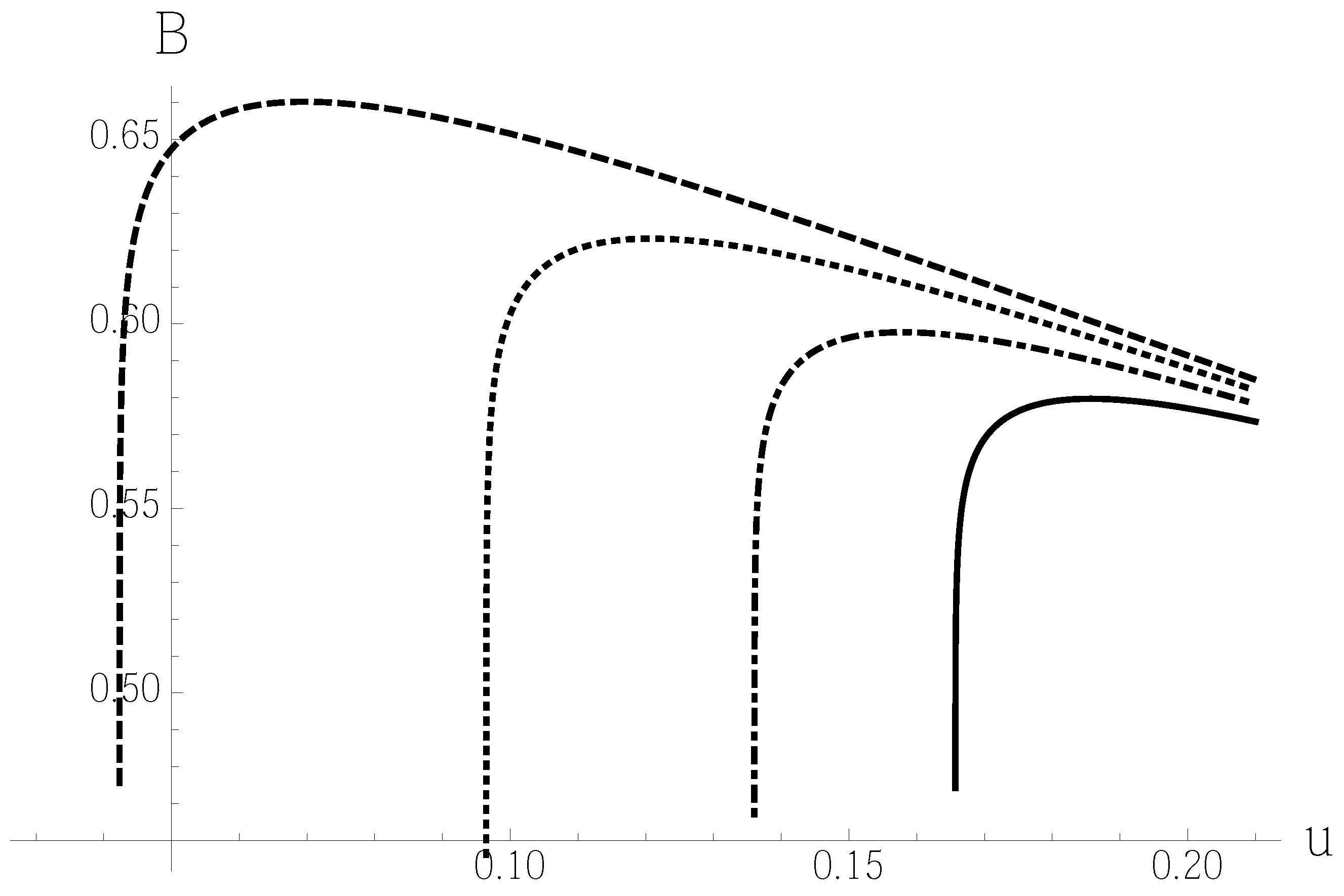
The problem appears to be difficult for the uncontrolled Borel method, and the high-order iterated roots both give complex results. However, by introducing controls, we can find good, real solutions to the minimal-derivative conditions (23), but not to the minimal-difference conditions. The behavior of amplitudes in higher orders are shown dependent on the parameter u in Figure 1, and various results by different methods are presented in the

Table 3. Energy Gap for the Schwinger Model. Dependencies on the approximation order. The exact value of the amplitude for the energy gap of the vector state equals 0.5642.

${\mathit{B}}_{\mathit{k}}$	7th	8th	9th	10th
Fractional Borel, (u-opt., $b=1$)	0.6602	0.6231	0.5978	0.5797
Borel ($u=0$, $b=1$)	complex	complex	complex	complex
Iterated Roots	complex	complex	complex	complex
Even Padé-Borel [17]		0.7027		0.7028
Odd Padé-Borel [17]	0.7023		0.70235
Even Padé [17]		0.7055		0.7138
Odd Padé [17]	0.7146		0.6999
Corrected Padé [38]		0.6915		0.6954

.

The best result previously, $B=0.5912$ with the error of $4.8\%$, was achieved by the method of corrected Padé approximants in the 14th order of perturbation theory [38]. The novel method gives better results, $B\approx 0.5797$, with the error of $2.75\%$ already in 10th order of perturbation theory. Note that finite lattice calculations give $B=0.57\left(1\right)$ [37], while various series methods give $B=0.56\left(2\right)$ [37].

5.3. Schwinger Model: Critical Amplitude

Consider the ground-state energy E of the Schwinger model. The expansions in the dimensionless coupling parameter x are known for the ground-state energy at small-x

$$E\left(x\right)\simeq 0.5642-0.219x+0.1907x^2(x\to 0),$$

(38)

and large-x

$$E\left(x\right)\simeq B{x}^{-1/3}(x\to \infty ),$$

with $B=0.6418$. Typically, we would add one more trial term with $a_3=0$ in the weak-coupling limit. The truncations and relevant discussion can be found in the papers [37,40,41,42,43,44,45].

Note that for negative $\beta$, we should consider the inverse of energies. Optimization with parameter u by imposing the minimal-difference condition $B_{3,1}\left(u_3\right)-B_{2,1}\left(u_2\right)=0,$ gives the control parameter $u_2=0.13435$; and we could find $B={B_{3,1}\left(u_2\right)}^{-1}=0.6672$.

In such a case, only minimalistic truncations in the dimensionless coupling parameter x are available and there is not much room for an improvement. The results of calculations by various methods are shown in the

Table 4. Schwinger Model: Amplitude.

Schwinger	Critical Amplitude
Fractional Borel ($b=1$, u-optimal)	0.6672
Odd Padé–Borel [17]	0.6122
Optimal Mittag–Leffler [9]	0.6202
Optimal Borel-Leroy [9]	0.6076
Optimal Generalized Borel [1]	0.6442
Borel ($u=0$, $b=1$)	0.6562
Modified Even Padé–Borel [17]	0.651
Exact	0.6418
Odd Padé [17]	0.5344
Iterated Roots, second order	0.5523

.

We want to stress here the usefulness of an approach based on attacking the problem by multiple methods. We also note that for such minimalistic truncation with only two nontrivial terms, the modified-even Padé–Borel technique with a special corrector given by the formula 4.8 from the paper [17] is still able to produce a good estimate $B=0.651.$ The u-optimal solution obtained above is not the best, but it is still quite reasonable. The best results are found from the Optimal Generalized Borel [1].

If in the case of a rather long truncation from the previous two examples, one can study the numerical convergence dependent on the approximation number. In the case of a short truncation, one has to rely on agreement among various methods of resummation. Additionally, in the particular case just presented, such an approach appears to be feasible.

5.4. Anomalous Dimension

In the $n=4$ supersymmetric Yang–Mills theory, the cusp anomalous dimension $\Omega \left(g\right)$ of a light-like Wilson loop, depends only on the coupling g (see [46] and references therein).

In terms of the variable $x=g^2$, the problem can be written down in terms of the function $f\left(x\right)=\frac{\Omega \left(x\right)}{x}$, with the following weak-coupling expansion,

$$f\left(x\right)\simeq 4-13.1595x+95.2444x^2-937.431x^3,x\to 0,$$

while in the strong-coupling limit $f\left(x\right)$ takes the form of a power-law

$$f\left(x\right)\simeq B{x}^{\beta },x\to \infty ,$$

with $B=2$ and $\beta =-1/2$.

Fractional Borel technique with minimal-difference condition (21) ($b=1,2$), has a unique solution

$$B_3\left(u_3\right)=1.90291,$$

for the u-optimization problem with very small optimal $u_3=0.0164826$. The result for the amplitude is quite reasonable, while the best result, $B=2.0118$, is delivered by the optimal Borel–Leroy summation discussed in the paper [9]. More results obtained by different methods are shown in the

Table 5. Cusp.

Cusp	Critical Amplitude
Fractional Borel ($b=1,2$, u-optimal)	1.90291
Odd Padé [17]	1.79734
Odd Padé–Borel [17]	2.06701
Optimal Borel–Leroy [9]	2.01177
Optimal Generalized Borel [1]	2.29603
Borel ($u=0$, $b=1$)	2.4416
Iterated Roots	1.69766
Exact	2

.

The problem was recently studied by means of various Padé and Padé–Borel techniques [17]. Only the best results are shown in the Table 5.

5.5. One-Dimensional Bose Gas: Amplitude

The ground-state energy $E\left(g\right)$ of the one-dimensional Bose gas with contact interactions depends only on the non-dimensional coupling parameter g. The expansion for the energy was found in high orders of perturbation theory [47,48]. In the variables $e\left(x\right)\equiv E\left(x^2\right),g\equiv x^2,$ the weak-coupling expansion is written as follows, for $x\to 0$,

$$\begin{array}{c}e\left(x\right)\simeq x^2(1-0.4244131815783876x+0.06534548302432888x^2-\hfill \\ 0.001587699865505945x^3-0.00016846018782773904x^4-\hfill \\ 0.00002086497335840174x^5-3.1632142185373668{10}^{-6}{x}^6-\hfill \\ 6.106860595675022{10}^{-7}{x}^7-1.4840346726187777{10}^{-7}{x}^8).\hfill \end{array}$$

(39)

In the limit of strong couplings, as $x\to \infty$, the celebrated exact result

$$E(\infty )=\frac{{\pi }^2}{3}\approx 3.289868.$$

(40)

is known due to Tonks and Girardeau (1960).

The better results can be achieved with addition to the (39) of the two more, very small trial terms

$$a_9=a_{10}=0.$$

Yet, various Padé and Padé–Borel approximations [17], fail beyond any way of repairing them by simple means.

Fractional Borel Summation provides a u-optimal solution to the Equation (21) ($b=1,2$). The values of the control parameter appear to be quite large, and are shown below,

$$u_7=1.10855,u_8=1.20477,u_9=1.2528,u_{10}=1.27757.$$

This is in contrast with rather small values of the control parameters found in previous examples. The result $B={\left(B_{10,2}\left(u_{10}\right)\right)}^{-1}=3.81457$ is not the best, but quite reasonable. It brings a significant improvement over the Borel summation as shown in

Table 6. Ground state energy for the one-dimensional Bose gas. Dependencies on the approximation order. The exact value of the amplitude for the energy equals $\frac{{\pi }^2}{3}\approx 3.28987$.

${\mathit{B}}_{\mathit{k}}$	7th	8th	9th	10th
Fractional Borel, (u-opt., $b=1,2$)	4.57557	4.31065	3.93828	3.81457
Borel ($u=0$, $b=1$)	4.70625	4.50604	4.35113	4.22934
Generalized (iterated) Borel [17]	3.31805	3.38914	3.40286	3.39967
Iterated Roots [9]	3.64329	3.52695	3.45274	3.40983

.

Let us also mention that the second-order iterated root corrected also with the iterated roots in the 8th order of perturbation theory [23], also gives a reasonable estimate of $B=3.77136$. The best, very close results in this case are achieved by some other methods. Various results are brought up in the Table 6. The method of optimal Mittag–Leffler summation gives in fact the same results as iterated roots [9] applied without any transformations.

5.6. Membrane: Pressure

In the case of a two-dimensional membrane, its pressure can be calculated by perturbation theory with respect to the wall stiffness characterized by the non-dimensional parameter g [49], so that

$$p_k\left(g\right)=\frac{{\pi }^2}{8g^2}\left(1+\sum _{n=1}^k{a}_n{g}^n\right),$$

(41)

with the coefficients

$$a_1=\frac{1}{4},a_2=\frac{1}{32},a_3=2.176347\times {10}^{-3},$$

$$a_4=0.552721\times {10}^{-4},a_5=-0.721482\times {10}^{-5},a_6=-1.777848\times {10}^{-6}.$$

The so-called rigid-wall limit corresponds to an infinite g. Most accurately, it is calculated by means of the Monte Carlo simulations [50]. The following value is considered as a benchmark:

$$p(\infty )=0.0798\pm 0.0003.$$

(42)

All Padé and overwhelming majority of Padé–Borel approximations fail miserably, at least in the given orders of perturbation theory. The results below are obtained with the addition of the two trial, very small terms with $a_7=a_8=0.$

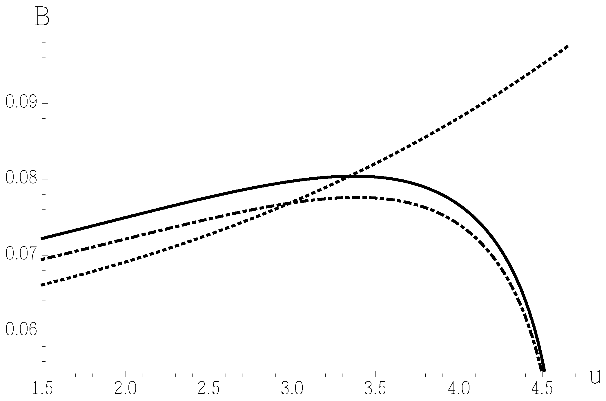
The dependencies of amplitudes on the control parameter u in higher orders of perturbation theory and $b=1$, are shown in Figure 2. Very good result, $B=0.08041$, is achieved in the 8th order with minimal-derivative condition. Additionally, a good result, $B=0.07761$, is achieved with a minimal-derivative condition imposed in the 7th order of perturbation theory.

The results obtained by various methods are shown in the

Table 7. Fluctuating membrane.

Membrane	Pressure
Fractional Borel, 7th order, (u-optimal, $b=1$)	0.0776132
Fractional Borel, 8th order, (u-optimal, $b=1$)	0.0804093
Odd Padé–Borel, 5th order	0.0832274
Borel, ($u=0$, $b=1$), 8th order	0.0651721
Corrected Padé Approximants [38]	0.0806101
Corrected Iterated Root Approximants [23]	0.0784338
Doubly renormalized iterated roots [24]	0.0792
Optimal perturbation theory  [49]	0.0821
Continued roots, 5th order [51]	0.07957
Continued roots, 6th order [51]	0.083702
Iterated Roots, 8th order	0.073258
“Exact” Monte Carlo	0.0798

.

We register a significant improvement over the Borel result $B=0.06517$. The former result is to be compared with the also reasonable value of $0.0821$ from the variational (optimal) perturbation theory [49].

The iterated root in 4th order corrected with iterated roots in the 8th order of perturbation theory, as described in the paper [23], also gives a reasonable estimate $p=0.0784338$.

6. Examples of b-Optimization

When even one of the two Hadamard conditions is not met in the course of u-optimization, we apply another complementary procedure of optimization with respect to another parameter, number of iterations b, extended to an arbitrary real number from the original integers [1]. When the solution to such a b-optimization problem exists and is unique, our task could be considered as completed. A few examples of a successful application of the b-optimization are presented below.

6.1. Two-Dimensional Polymer: Amplitude

For the swelling factor $\mathsf{{\rm Y}}$ of the two-dimensional polymer coil, perturbation theory yields the expansion in powers of the dimensionless coupling parameter g [52],

$$\mathsf{{\rm Y}}\left(g\right)\simeq 1+\frac{1}{2}g-0.12154525g^2+0.02663136g^3-0.13223603g^4,$$

(43)

as $g\to 0$. As $g\to \infty$, the swelling factor behaves as a power-law, i.e.,

$$\mathsf{{\rm Y}}\left(g\right)\simeq B{g}^{\beta }.$$

The index at infinity $\beta =1/2$ is considered to be known exactly [53,54]. The amplitude B is of the order of unity.

Since there is no solution to the u-optimization problem, we resort to the fractional Borel method with b-optimization and $u=0$. By applying the minimal-difference condition, $B_4\left(b_3\right)-B_3\left(b_3\right)=0,$ the method brings the following estimate

$$B=B_4\left(b_3\right)=0.9707,$$

with $b_3=0.8361327$. The results obtained by various methods are presented in the

Table 8. Expansion factor of the two-dimensional polymer.

$2\mathit{d}$ Polymer	Critical Amplitude
Fractional Borel ($u=0$, b-optimal)	0.970678
Even Padé [17]	1.00002
Even Padé–Borel [17]	0.977767
Optimal Borel–Leroy ($b=1$) [9]	1.14311
Optimal Borel–Leroy ($b=1,2$) [9]	1.14344
Optimal Generalized Borel ($b=1$) [1]	0.968895
Optimal Generalized Borel ($b=1,2$) [1]	0.954187
Borel ($b=1$, $u=0$)	0.969559
Iterated Roots, third order	0.970718
Iterated Roots, 4th order	complex
“Exact” conjectured	1

. Except for the results of Borel–Leroy summation, they are all close to unity.

6.2. Three-Dimensional Polymer: Amplitude

Similarly, a perturbation theory for the expansion factor of a three-dimensional polymer coil leads to a series in a single dimensionless parameter g, which measures the repulsive interaction between segments of the polymer [52,55]. As $g\to 0$, the expansion factor $\mathsf{{\rm Y}}\left(g\right)$ can be presented as the truncated series similar, at first glance, to the case of an anharmonic oscillator, with the coefficients

$$a_0=1,a_1=\frac{4}{3},a_2=-2.075385396a_3=6.296879676,$$

$$a_4=-25.05725072,,a_5=116.134785,a_6=-594.71663.$$

The strong-coupling behavior of the expansion factor as $g\to \infty$, is power-law

$$\mathsf{{\rm Y}}\left(g\right)\simeq B{g}^{\beta }.$$

The parameters B and $\beta$ above were found numerically in the paper [55]. It is known [55] that $B\approx 1.531$, while $\beta \approx 0.3544$.

With fixed critical index $\beta$, we calculate critical amplitude B by various methods based on the expansion for small g. The results of calculations with different methods are shown in the

Table 9. Expansion factor of the three-dimensional polymer.

$3\mathit{d}$ Polymer	Critical Amplitude
Fractional Borel, 6th order, ($u=0$, b-optimal)	1.53523
Even Padé, 6th order [17]	1.54022
Even Padé–Borel [17]	1.53296
Odd Padé, 5th order [17]	1.54089
Odd Padé–Borel [17]	1.52996
Iterated Roots, 6th order	1.53611
Borel, 6th order, ($b=1$, $u=0$)	1.52718
“Exact” numerical	1.5309

.

A fractional, b-optimal, Borel technique of 6th order with $u=0$, with the minimal-difference condition, $B_6\left(b_5\right)-B_5\left(b_5\right)=0,$ gives

$$B_6\left(b_5\right)=1.53523,$$

with $b_5=0.290422$; and the result is good. The best, most consistent results, however, are delivered by the Padé–Borel techniques of the paper [17]. They seem to bracket the numerical result.

6.3. One-Dimensional Nonlinear Model

Quantum properties of the Bose-condensed atoms in a harmonic trap are modelled by the the one-dimensional stationary nonlinear Schrödinger equation. The energy levels are represented in the form $E\left(g\right)=\left(n+\frac{1}{2}\right)f\left(g\right),$ where $n=0,1,2,\dots$ is a quantum index and g is a dimensionless coupling parameter quantifying the effect of trapping. The perturbation theory for the function $f\left(g\right)$, gives the expansion $f\left(g\right)=1+{\sum }_{n=1}^k{a}_n{z}^n$ in powers of g. The coefficients $a_n$ can be found in the paper [24]:

$$a_1=1,a_2=-\frac{1}{8},a_3=\frac{1}{32},a_4=-\frac{1}{128},a_5=\frac{3}{2048}.$$

And one more coefficient, very small $a_6=0$, can be tried in order to improve accuracy.

For the strong-coupling limit, we have a power-law

$$f\left(g\right)\simeq B{g}^{\beta },$$

with $B=\frac{3}{2}$, $\beta =\frac{2}{3}$.

As demonstrated below, the solutions for B suggested by the two optimization conditions in the 4th order are very close to each other. This is exactly what one would expect from the two different optimization conditions imposed on the amplitudes.

With a fractional, b-optimal, Borel technique with minimal-difference condition, by applying the minimal-difference condition, $B_5\left(b_4\right)-B_4\left(b_4\right)=0,$ we obtain

$$B=B_5\left(b_4\right)=1.46952,$$

with $b_4=-1.01704$.

A fractional, b-optimal, Borel technique with minimal-derivative condition, $\frac{\partial B_4\left(b_4\right)}{\partial b_4}=0,$ gives

$$B=B_4\left(b_4\right)=1.47592,$$

with $b_4=-1.28859$.

The results of both optimizations are quite reasonable, while the best results are delivered by the Padé techniques of the paper [17]. The results obtained by various methods are presented in the

Table 10. Nonlinear quantum model.

$1\mathit{d}$ Nonlinear Model	Critical Amplitude
Fractional Borel, 4th order, minimal derivative, b-opt.	1.47592
Fractional Borel, 5th order, minimal difference, b-opt.	1.46952
Odd Padé, 5th order [17]	1.49226
Odd Padé–Borel, 5th order [17]	1.57327
Even Padé, 4th order [17]	1.49181
Even Padé–Borel, 4th order [17]	1.56761
Borel, 5th order ($b=1$, $u=0$)	1.38512
Iterated roots, 5th order	1.44795
Continued roots, 5th order [51]	1.523478
Exact	3/2

. Almost all of them, excepting the method of Borel summation, are good.

6.4. Three-Dimensional Trap

The wave function $\psi \left(r\right)$ of the Bose-condensed atoms in a spherically symmetric harmonic trap can be found from the three-dimensional stationary nonlinear Schrödinger Equation [56]. The problem can be reduced to studying only the radial part of the condensate wave function

$$\chi \left(r\right)=\frac{1}{2{\pi }^{1/2}}\frac{\psi \left(r\right)}{r},$$

with $\chi \left(0\right)=0$. The latter function is defined by the effective nonlinear Hamiltonian [56]

$${\widehat{H}}_r=\frac{1}{2}\left(-\frac{d^2}{d{r}^2}+r^2\right)+\frac{g}{4\pi r^2}{\chi }^2,$$

(44)

where g is a dimensionless coupling parameter. The function $\chi \left(r\right)$ can be obtained from the effective three-dimensional stationary nonlinear Schrödinger Equation [56], or else to the ODE

$${\widehat{H}}_r\chi =E\chi ,$$

where E stands for the sought ground-state energy. More examples and references to ODEs from quantum mechanics and polymers can be found in the reviews [24,56]. Sometimes, more complicated PDEs can be reduced to the cascades of ODEs [57]. The solutions to PDEs when homogenized lead to various expansions of effective transport coefficients, which can be resummed by various methods including Borel summation [58]. See multiple examples of similar problems in the paper by Gluzman, Symmetry (2022), on asymptotics and summation of the effective properties of suspensions, liquids and composites. It could be also interesting to apply the novel “Borelian” methods to the various problems of aero-and-hydrodynamics [59,60].

Finally, the ground state energy E of the trapped Bose-condensate can be approximated by the following truncation expressed in terms of the parameter $c\equiv \frac{2g}{{\left(2\pi \right)}^{3/2}}$,

$$E\left(c\right)\simeq \frac{3}{2}+\frac{1}{2}c-\frac{3}{16}{c}^2+\frac{9}{64}{c}^3-\frac{35}{256}{c}^4,(c\to 0),$$

(45)

where c quantifies the effect of trapping.

On the other side, the energy behaves as the power-law

$$E\left(c\right)\simeq B{c}^{\beta },(c\to \infty ),$$

(46)

with the amplitude at infinity $B=\frac{5}{4}$, and index $\beta =2/5$ [56].

Fractional, b-optimal, Borel technique with minimal-difference condition, in the 4th order gives

$$B=B_4\left(b_3\right)=1.2852,$$

with $b_3=0.9504$.

The results from various methods are presented in

Table 11. Three-dimensional trap.

Trap	Critical Amplitude
Fractional Borel, minimal difference, b-optimal	1.28517
Odd Padé [17]	1.3097
Odd Padé–Borel [17]	1.29394
Even Padé [17]	1.28211
Even Padé–Borel, 2nd order [17]	1.23729
Even Padé–Borel, 4th order [17]	1.28548
Borel ($u=0$, $b=1$)	1.28492
Optimal Borel–Leroy ($b=1$) [9]	1.28664
Optimal Generalized Borel ($b=1$) [1]	1.28459
Iterated roots	1.27392
Exact	5/4

. All of them give close and good enough results. The results for iterated roots are also Mittag–Leffler optimal. The method of Even Padé–Borel approximants [17], gives a good estimate from below and from above, as shown in Table 11.

7. Bose Temperature Shift

In the cases when even one of the two Hadamard conditions are not met in the course of u- and b-optimizations of the complete amplitude B, we suggest applying yet another procedure. Optimization is going to be applied to the marginal amplitude C, either with respect to the parameter u or parameter b with a subsequent correction by means of the diagonal Padé approximants [9]. The resulting approximation is going to satisfy asymptomatically the original truncated series (1) and (2).

The shift $\Delta T_c\equiv T_c-T_0$, of the Bose–Einstein condensation temperature $T_c$ of a non-ideal Bose system compared to the Bose–Einstein condensation temperature $T_0$ of ideal uniform Bose gas, is believed to have a simple form. At asymptotically small gas parameter $\gamma \equiv {\rho }^{1/3}{a}_s,$ where $a_s$ is atomic scattering length and $\rho$ stands for the gas density, it behaves as $\frac{\Delta T_c}{T_0}\simeq c_1\gamma ,$ for $\gamma \to 0$. Thus, the parameter $c_1$ quantifies the shift.

Monte Carlo simulations [61,62,63] give

$$c_1=1.3\pm 0.05.$$

(47)

At the same time, $c_1$ can be defined [64,65,66] as the strong-coupling limit

$$c_1=\underset{g\to \infty }{lim}{c}_1\left(g\right)\equiv B$$

(48)

of an auxiliary function $c_1\left(g\right)$. The latter function could be expressed as an expansion over an effective coupling parameter,

$$c_1\left(g\right)\simeq a_{1}g+a_2{g}^2+a_3{g}^3+a_4{g}^4+a_5{g}^5,$$

(49)

where

$$a_1=0.223286,a_2=-0.0661032,a_3=0.026446,$$

$$a_4=-0.0129177,a_5=0.00729073.$$

Note that in the present case, in the actual problem solved for the auxiliary function $c_1\left(g\right)$, the index at infinity $\beta =-1$.

In the same way as in the case of the Bose system, one can find the values of $c_1$ for the $O\left(1\right)$ field theory [65]. The following, formally obtained expansion is available the auxiliary function for small g,

$$c_1\left(g\right)\simeq 0.334931g-0.178478g^2+0.129786g^3-0.115999g^4+0.120433g^5.$$

The Monte Carlo numerical estimate $c_1=1.09\pm 0.09,$ is available here as well (see [38] and references therein).

For the $O\left(4\right)$ field theory, analogous computations can be accomplished. The expansion for the auxiliary function $c_1\left(g\right)$ as $g\to 0$ can be found in [65], i.e.,

$$c_1\left(g\right)\simeq 0.167465g-0.0297465g^2+0.00700448g^3-0.00198926g^4+0.000647007g^5.$$

The Monte Carlo numerical estimate $c_1=1.6\pm 0.1,$ is available (see [38] and references therein).

The problem appears to be very difficult and even challenging for the Fractional Borel methodology, since the optimization in the parameter $u>0$ does not bring a solution, and optimization in the parameter b brings multiple (two) solutions. In such a case, the results could be found from the simplified, Borel-light summation introduced in the Section 4. Note that it is marginal amplitudes that have to be optimized. Note also that even in the case of $\beta =-1$, the Borel-light summation can be applied to the original series, without a need for inverting the truncations.

For example, in the case of Bose-condensate, the method of u-optimization with optimal $u_2=-0.31805$, found from the minimal difference condition $C_3\left(u_2\right)-C_2\left(u_2\right)=0,$ gives

$$B_{2,2}^{*}\left(u_2\right)\simeq P_{2/2}(\infty )C_2\left(u_2\right)=1.3085.$$

Here, and only here, we have to resort to a negative control parameter. The option of resorting to negative u when a positive solution does not present itself is quite straightforward, but seems to work well only in some special cases.

Similarly, the method of b-optimization with optimal $b_3=0.29893$, found from the minimal difference condition $C_4\left(b_3\right)-C_3\left(b_3\right)=0,$ gives

$$B_{2,4}^{*}\left(b_3\right)\simeq P_{2/2}(\infty )C_4\left(b_3\right)=1.2661.$$

Even without optimization, just setting $b=1$, $u=0$, we obtain the rather reasonable result

$$B_{2,4}^{*}\left(1\right)\simeq P_{2/2}(\infty )C_4\left(1\right)\approx 1.25.$$

The results of simplified, Borel-light summation introduced in Section 4, are further elaborated in

Table 12. Shift of the Bose-Einstein condensation temperature and analogous models. Borel-light methodology.

Parameter ${\mathit{c}}_1$	Bose	$\mathit{O}\left(1\right)$	$\mathit{O}\left(4\right)$
Fractional Borel-light ($u=0$, b-optimal)	1.2498	1.0792	1.4862
Fractional Borel-light ($b=1$, u-optimal)	1.3085	1.1394	1.5268
Fractional Borel-light ($u=0$, $b=1$)	1.2661	1.1005	1.4796

. The results obtained by the Fractional Borel-light ($b=1$, u-optimal), seem to be more in line with the other two preferred estimates.

Various results for all three cases obtained by different methods are shown in the

Table 13. Shift of the Bose–Einstein condensation temperature and analogous models.

Parameter ${\mathit{c}}_1$	Bose Condensate	$\mathit{O}\left(1\right)$	$\mathit{O}\left(4\right)$
Fractional Borel-light	1.24977	1.07921	1.48618
Modified-Even Padé [17]	1.28853	1.11459	1.51825
Corrected Iterated Roots [23]	1.30915	1.13817	1.5238
Optimal Mittag–Leffler [9]	1.33967	1.14124	1.60226
Optimal Generalized Borel [1]	1.33898	1.15286	1.57478
“Exact” Monte Carlo	1.3 ± 0.05	1.09 ± 0.09	1.6 ± 0.1
Odd Padé [17]	0.985	0.82441	1.218855
Borel ($u=0$, $b=1$)	1.54664	1.35492	1.75813
Iterated Roots	complex	complex	complex

.

We comment that the simplest approaches of Modified-Even Padé approximants of the [17], and Corrected Iterated Root Approximants of the paper [23], give close and good results, and without any explicit optimization or transformation of the series being imposed. In such a sense, they are preferable to others.

For instance, the second-order iterated roots corrected with iterated roots in the 4th order of perturbation theory, as described in the paper [23], gives reasonable estimates in all three cases. The corresponding results are shown in the third line of the Table 13. In particular, for the Bose-condensation, the method of corrected iterated roots gives $c_1=1.30915$.

Kastening [64,65,66], using the Kleinert variational perturbation theory, found the Bose-condensation problem the value of $c_1$ in the interval 1.16 – 1.38; and estimated the shift as $1.27\pm 0.11$.

8. Case of β = 0

In order to address the case of $\beta =0$, the definition of iterated roots should be modified slightly. Conditioning the approximants on correct critical exponent $\beta =0$ at infinity, we suggest the modified iterated root approximants in the form

$$r_k\left(x\right)=a_0+{\mathcal{P}}_{1}x{\left({\left({\left({(1+{\mathcal{P}}_{2}x)}^2+{\mathcal{P}}_3{x}^2\right)}^{3/2}+{\mathcal{P}}_4{x}^3\right)}^{4/3}+\dots +{\mathcal{P}}_k{x}^k\right)}^{\alpha /k},$$

(50)

with known powers and unknown amplitudes. The number of unknowns is exactly the same as for the iterated roots described in the Section 1.1.

We request that

$$1+\alpha =\beta ,$$

(51)

so that in the case of $\beta =0$, one finds that $\alpha =-1$ in all orders $k=2,3,\dots$. For instance, for $k=2$ the approximant (8) is simply

$$r_2\left(x\right)=a_0+{\mathcal{P}}_{1}x{\left(1+{\mathcal{P}}_{2}x\right)}^{-1},$$

(52)

for $k=3$

$$r_3\left(x\right)=a_0+{\mathcal{P}}_{1}x{\left({\left(1+{\mathcal{P}}_{2}x\right)}^2+{\mathcal{P}}_3{x}^2\right)}^{-\frac{1}{2}},$$

(53)

and for $k=4$

$$r_4\left(x\right)=a_0+{\mathcal{P}}_{1}x{\left({\left({\left(1+{\mathcal{P}}_{2}x\right)}^2+{\mathcal{P}}_3{x}^2\right)}^{3/2}+{\mathcal{P}}_4{x}^3\right)}^{-\frac{1}{3}},$$

(54)

Now, all relevant parameters ${\mathcal{P}}_j$ could be uniquely defined from the asymptotic equivalence with the truncated series $f_k\left(x\right)$ in the small x limit. Of course, the approximants can be (and will be) applied also to the Borel-type transformed series as well.

In the large-variable limit, the approximant (50) behaves as

$$r_k\left(x\right)\simeq C_k(x\to \infty ),$$

(55)

with the critical amplitude

$$C_k=a_0+{\mathcal{P}}_1{\left({\left({\left({\mathcal{P}}_2^2+{\mathcal{P}}_3\right)}^{3/2}+{\mathcal{P}}_4\right)}^{4/3}+\dots +{\mathcal{P}}_k\right)}^{-1/k}.$$

(56)

The large-variable exponent $\beta =0$ of the sought function $f_k^{*}\left(x\right)$ coincides with that for the self-similar Borel transform $r_k^{*}\left(x\right)$. However, the transform $r_i^{*}\left(x\right)$ with $i=2,3,\dots k$ is different from the sought function $f_i^{*}\left(x\right)$.

In what follows, we adhere to the logic of the Section 4, outlined for the Borel-light summation. In the case of u-optimization, in order to establish an inverse transform to original series, instead of taking the integral, the sought function can be reconstructed directly and explicitly, as suggested in Section 4, i.e.,

$$f_{n,i}^{*}\left(x\right)\simeq P_{n/n}\left(x\right)r_i^{*}\left(x\right),$$

(57)

with $i=2,3,\dots ,k$. While $n=1,2\dots k/2$ for even k, and $n=1,2,\dots ,(k-1)/2$ for odd k. The parameters of the diagonal Padé approximant are to be found from the accuracy-through-order procedure [67], from asymptotic equivalence with the original expansions (2) and (3).

Assume that the number of iterations b is fixed and does not appear in the forthcoming formulas. At large values of the variable, the self-similar Borel-type transform behaves as

$$r_i^{*}(x,u)\simeq C_i\left(u\right)(x\to \infty ),$$

(58)

and the total critical amplitude

$$B_{n,i}^{*}\left(u_i\right)\simeq P_{n/n}(\infty )C_i\left(u_i\right),$$

(59)

ought to be calculated. The parameter $u=u_i$ is to be found from the minimal derivative condition, as the unique solution to the equation

$$\frac{\partial C_i\left(u_i\right)}{\partial u_i}=0,$$

(60)

or from the minimal difference condition, with the differences

$$C_{i+1}\left(u_i\right)-C_i\left(u_i\right)=0,$$

(61)

and for positive integers $i=2,3,\dots ,k$. The optimization similar to the equation (21) can be written down as well by simply changing notations.

The control parameter can be also fixed to the value $u=0$, and the same procedures can be applied with respect to the number of iterations b [1]. Equations (59)–(61) will hold with u simply replaced by b.

Of course, the approximants (50), with the condition (51), can also be applied when $\beta \ne 0$.

8.1. One-Dimensional Antiferromagnet: Ground State Energy

The ground-state energy of an equilibrium one-dimensional quantum Heisenberg antiferromagnet can be found [68] from the energy $E\left(t\right)$ of a non-equilibrium antiferromagnet. At small time $t\to 0$, one has an expansion

$$E\left(t\right)\simeq -\frac{1}{4}\left(1+\sum _{n=1}^4{a}_n{t}^n\right),$$

(62)

with the coefficients

$$a_1=4,a_2=-8,a_3=-\frac{16}{3},a_4=64.$$

However, it is the infinite time limit $E(\infty )$ that ought to be deduced from the expansion (62). The ground-state energy is known exactly due to Hulthen [69],

$$E=E(\infty )=-0.4431.$$

(63)

The u-optimization-light procedure fails to bring a reasonable solution. The b-optimization procedure with $u=0$, returns us to the case of iterative Borel summation [1]. Solving the equation $C_4\left(b_3\right)-C_3\left(b_3\right)=0,$ brings a unique solution $b_3=-0.42432$. Accomplishing inverse integral transformation is quite straightforward since the contribution from $\Gamma$-term equals unity in the case of $\beta =0$. It gives the amplitude, which is equal to the marginal amplitude. From the marginal amplitude, we simply estimate that

$$E(\infty )\approx B_4=C_4\left(b_3\right)=-0.441343.$$

In the method of Borel-light described above, the b-optimal marginal amplitude found with $b_3=-0.42432$, $u=0$, ought to be corrected with the diagonal Padé approximants. Simply rewriting the formula (59) for b in place of u leads to the total critical amplitude

$$B_{2,4}^{*}\left(b_3\right)=P_{2/2}(\infty )C_4\left(b_3\right)=-0.464547.$$

A slightly different result is achieved by calculating

$$B_{1,4}^{*}\left(b_3\right)=P_{1/1}(\infty )C_4\left(b_3\right)=-0.441343,$$

which is exactly the result achieved by the inverse integral transformation.

Various approximations are shown in

Table 14. Antiferromagnet.

$1\mathit{d}$ Antiferromagnet	Energy
Fractional Borel, u = 0, b-optimal	−0.4413
Fractional Borel-light	−0.4645
Odd-Factor Approximants [70]	−0.4452
Iterated Root Approximants (50)	−0.4819
Exact (Hulthen)	−0.4431
Diagonal Padé, 2th order	−0.75
Diagonal Padé, 4th order	−0.3289
Borel ($u=0$, $b=1$)	−0.6821

. Note that by applying the minimal-derivative condition to optimal Mittag–Leffler summation [9] with odd-factor approximants of [70], one can see that our very good estimator, the simple odd-factor approximant, is also Mittag–Leffler-optimal.

The diagonal Padé approximation and the Borel approximation ($u=0$, $b=1$) are inferior performers individually, but could be viewed as upper and lower bounds on the solution.

8.2. Fermi Gas: Unitary Limit

The ground-state energy E of a dilute Fermi gas can be obtained perturbatively [71], so that

$$E\left(g\right)\simeq a_0+a_{1}g+a_2{g}^2+a_3{g}^3+a_4{g}^4,$$

(64)

with the coefficients

$$a_0=\frac{3}{10},a_1=-\frac{1}{3\pi },a_2=0.055661,$$

$$a_3=-0.00914,a_4=-0.018604.$$

The expansion (effective coupling) parameter $g\equiv |k_F{a}_s|,$ is expressed through the Fermi wave number $k_F$ and the atomic scattering length $a_s$. The limit of very large g corresponds to the unitary Fermi gas. Monte-Carlo numerical calculations in the case of $g\to \infty$ [72,73] yield

$$E(\infty )=0.1116.$$

(65)

More recent Monte Carlo simulations give a slightly higher value of $E(\infty )=0.1164$ [74]. The best known experimental value is equal to

$$E(\infty )=0.1128,$$

according to [72,75].

Let us consider the inverse of the truncated series (64), and apply to it various resummation procedures. The transformation allows us to remove the spurious zeroes at the real axis, which severely worsens the results for the original truncation.

In this case, u-optimization could be performed with $b=1$. The u-optimal marginal amplitude is found from the equation $C_4\left(u_3\right)-C_3\left(u_3\right)=0,$ which gives $u_3=0.1532$. After correction with the diagonal Padé approximant, we find $B_{2,4}^{*}\left(u_3\right)=P_{2/2}(\infty )C_4\left(u_3\right),$ and estimate after inversion that $E(\infty )\approx 0.1256$.

Slightly lower result, $E(\infty )\approx 0.1244$, is achieved by calculating an inverse of the amplitude $B_{1,4}^{*}\left(u_3\right)=P_{1/1}(\infty )C_4\left(u_3\right).$

For completeness, let us also consider the b-optimal optimization procedure with $u=0$. Solving the equation $C_4\left(b_3\right)-C_3\left(b_3\right)=0,$ brings a unique solution $b_3=0.90885$. The amplitude is equal to the marginal amplitude, $B_4=C_4\left(b_3\right).$ After inversion, we find that $E(\infty )\approx 0.1367.$

Another way to introduce control consists in replacing the exponential function in the integrand of the formula (4), by a stretched (compacted) exponential function, parameterized with the parameter U [1]. Applying the same technique of Borel-light summation as above, we find from the minimal difference condition $C_4\left(U_3\right)-C_3\left(U_3\right)=0,$ a uniquely defined control parameter $U_3=1.12197$. After calculating the amplitude $B_{2,4}^{*}\left(U_3\right)=P_{2/2}(\infty )C_4\left(U_3\right),$ and taking its inverse we find

$$E(\infty )\approx 0.119305.$$

Thus, the best result, $E=0.1193$, achieved previously by the Borel-Factor Approximants-light technique applied to the Mittag–Leffler transformed series [9], is reproduced.

Various approximations are shown in the

Table 15. Fermi gas.

Unitary Limit	Energy
Fractional Borel—light, fourth order, u-optimal	0.1256
Fractional Borel—light, second order, u-optimal	0.1244
Fractional Borel, u = 0, b-optimal	0.1367
Corrected—Factor Approximants [70]	0.1434
Corrected—Iterated Roots Approximants [24]	0.1029
Borel—Factor Approximants-light [9]	0.1193
Generalized Borel—light, fourth order, U-optimal [1]	0.1193
Diagonal Padé, 2th order	0.09774
Diagonal Padé, 4th order	0.1705
Iterated Root Approximants  (50)	0.1627
Borel (u = 0, $b=1$)	0.1329
“Exact” Monte Carlo [72,73]	0.1116

. Thus, Borel-light techniques of various shades work well for the unitary limit of Fermi gas.

9. Discussion of Some Future Directions

For future work, with the goal to improve the behavior of the coefficients of transformed series in mind, one can consider the following generalization of Borel-transformed series:

$$A_k(x,\omega )=\sum _{n=0}^k\frac{a_n{(1+n)}^{\omega }}{\Gamma (1+n)}{x}^n,$$

(66)

where the parameter $\omega$ could be arbitrary in principle. The formula (66) appears to be well-defined as $n=0$. For negative $\omega$ and large n, the behavior of transformed quantities (66) is similar to that of (5).

Additionally, let us introduce the following operator:

$$I\left(t\right)=t^{-1}{\int }_0^{t}d\tau \left[\right].$$

(67)

The result of application of operator $I\left(t\right)$ to the power-law $f\left(t\right)=t^{\beta }$ is a simple division of the $f\left(t\right)$ by the factor $\beta +1$. The operator can be used to define an inverse transformation. Then, the sought function is approximated by the expression $f_k^{*}(x,\omega )={\int }_0^{\infty }{e}^{-t}{I\left(t\right)}^{\omega }\left[R_k^{*}(xt,\omega )\right]dt,$ while the amplitude

$$B_k\left(\omega \right)=C_k\left(\omega \right){\left(1+\beta \right)}^{-\omega }\Gamma (\beta +1).$$

(68)

The latter formula appears to be well-defined as $\beta =0$. For negative $\omega$ and large $\beta$ the behavior of amplitudes (68) is similar to that of (11). The summation of such a type will be studied elsewhere.

Well-known Riemann–Liouville fractional derivative $D^u$ can be employed as well. However, it has to be multiplied by the powers $t^u$ to compensate for the changing powers in the course of differentiation, so that

$$t^u{D}^u{t}^{\beta }=\frac{\Gamma (1+\beta )}{\Gamma (1+\beta -u)}{t}^{\beta }.$$

(69)

A correspondent modification of the Borel-type transformation should be made, with a $\Gamma$-functional replacement of the power-law

$$n^u\Rightarrow \frac{\Gamma (1+n)}{\Gamma (1+n-u)},$$

in the transformation (5), along the lines of the papers [76,77]. Asymptotically, as $n\to \infty$ the two expressions above become equivalent. The corresponding amplitude is given as follows

$$B_k\left(u\right)=C_k\left(u\right)\frac{\Gamma {(\beta +1)}^2}{\Gamma (1+\beta -u)}.$$

(70)

The operators (6), (67) and (69) are designed specifically to respect the asymptotic power-law (1), or the so-called asymptotic scale-invariance of the sought functions.

Factor approximants [24] can be used in place of iterated roots. Despite clear technical complications arising in the course of analytical calculations with factors, they have the advantage of generality by including the case of $\beta =0$ automatically. Such a comparative study of the two different approximants is pending.

The standard Padé approximants are not sufficient for the set of problems exhibited in the paper, either not bringing a good enough accuracy or failing altogether. But their strength can be enhanced by adding not-so-complicated modifications [17], as can be seen from the numerical evidence. Still, there are some hard problems where even such enhanced Padé approximations are not sufficient and one has to be creative with some post-Padé methods.

Thus, the program for the near future consists of investigating resummation with various extensions of fractional derivatives. It is also necessary to study the methods of summation with factor approximants in place of iterated roots.

10. Conclusions

Our approach to optimization is inspired by the complementarity principle in physics. In a broad sense, an asymptotic complementarity principle [78], implies a deep connection between the limit of small and large variables.

The complete resummation procedure by the Fractional Borel Summation would require rather difficult from the technical standpoint optimization with respect to both u (fractional order of the operator $d{\left(t\right)}^u$ given by (6)) and b (fractional number of iterations first introduced in [1]). The optimization procedure when only parameter u is considered and b is fixed is called above u-optimization. The optimization procedure when only parameter b is considered and u is fixed is called above b-optimization. The problem could be treated in some cases only with u-optimization, or just with a b-optimization in some other cases. Neither of optimizations is able to solve overly many cases, but applied together they can and do complement each other.

Thus, we offer a shift in paradigm: instead of looking for a single method which can solve all the problems of resummation with reasonably good accuracy we suggest searching for complementary methods. In the course of u-optimization we search for the correction to factorial growth in the form of a fractional power, outside of the $\Gamma$-function. In the course of b-optimization we consider fractional powers of the $\Gamma$-function and optimize such powers. Considering only the one-parametric problems of optimization is technically and conceptually advantageous, compared to the two-parametric problems. The most interesting, as we see it, cases with the coefficients $a_n$ growing (decaying) very fast are covered neatly by the u-optimization. The cases of slower growing (decaying) coefficients are covered by b-optimization. The stand-alone resummation case is best tackled with Borel-light techniques.

The method of scale-invariant Fractional Borel Summation consists of three constructive steps. The first step corresponds to u-optimization of the amplitudes with fixed parameter b. When the first step fails, the second step corresponds to b-optimization of the amplitudes with fixed parameter u. However, when the two steps fail consecutively, the third step corresponds to Borel-light technique with marginal amplitude optimized with either of the two above approaches and corrected with a diagonal Padé approximants.

To assess the quality of approximation by the new methods, the pool of examples was selected to include various behaviors of the coefficients $a_n$. The method of Fractional Borel Summation appears to be a good, middle-off-the-road technique, allowing us to consider with relatively minor modifications all examples presented in the paper. Of course, in some important cases, the Fractional Borel method can be the best. We should stress that Fractional Borel Summation is the best among all analytical methods for such hard problems as quartic oscillator, various energy gaps for the Schwinger model and membrane pressure. For the two-dimensional polymer the value of amplitude is not known and the predictions are made. In the important cases of membrane pressure and of one-dimensional Bose gas energy various Padé and Padé–Borel techniques fail, while Fractional Borel Summation still works.

However, in general, to achieve the best results for a concrete problem of interest, one should turn to a variety of old or new methods. Among them, we can find the best method for the particular problem. However, if applied individually, each of the methods could be successful in just a few cases. Especially, when the Hadamard condition of uniqueness is imposed. Of course, there is a separate and non-trivial problem of deciding in real studies, which method is the best. That is why, possessing a well-defined methodology, such as the Fractional Borel Summation is important.

References

- Gluzman, S. Iterative Borel Summation with Self-Similar Iterated Roots. Symmetry 2022, 14, 2094. [Google Scholar] [CrossRef]
- Bender, C.M.; Boettcher, S. Determination of f(∞) from the asymptotic series for f(x) about x = 0. J. Math. Phys. 1994, 35, 1914–1921. [Google Scholar] [CrossRef]
- Bender, C.M.; Orszag, S.A. Advanced Mathematical Methods for Scientists and Engineers I: Asymptotic Methods and Perturbation Theory; Springer: New York, NY, USA, 1999. [Google Scholar]
- Suslov, I.M. Divergent Perturbation Series. J. Exp. Theor. Phys. 2005, 100, 1188–1233. [Google Scholar] [CrossRef]
- Sidi, S. Practical Extrapolation Methods; Cambridge University Press: Cambridge, UK, 2003. [Google Scholar]
- Graffi, S.; Grecchi, V.; Simon, B. Borel summability: Application to the anharmonic oscillator. Phys. Lett. B 1970, 32, 631–634. [Google Scholar] [CrossRef]
- Simon, B. Twelve tales in mathematical physics: An expanded Heineman prize lecture. J. Math. Phys. 2022, 63, 021101. [Google Scholar] [CrossRef]
- Antonenko, S.A.; Sokolov, A.I. Critical exponents for a three-dimensional O(n)-symmetric model with n>3. Phys. Rev. E 1995, 51, 1894–1898. [Google Scholar] [CrossRef]
- Gluzman, S. Optimal Mittag–Leffler Summation. Axioms 2022, 11, 202. [Google Scholar] [CrossRef]
- Mera, H.; Pedersen, T.G.; Nikolić, B.K. Nonperturbative quantum physics from low-order perturbation theory. Phys. Rev. Lett. 2015, 115, 143001. [Google Scholar] [CrossRef]
- Alvarez, G.; Silverston, H.J. A new method to sum divergent power series: Educated match. J. Phys. Commun. 2017, 1, 025005. [Google Scholar] [CrossRef]
- Mera, H.; Pedersen, T.G.; Nikolić, B.K. Fast summation of divergent series and resurgent transseries in quantum field theories from Meijer-G approximants. Phys. Rev. D 2018, 97, 105027. [Google Scholar] [CrossRef]
- Shalabya, A.M. Weak-coupling, strong-coupling and large-order parametrization of the hypergeometric-Meijer approximants. Results Phys. 2020, 19, 103376. [Google Scholar] [CrossRef]
- Sanders, S.; Holthau, M. Hypergeometric continuation of divergent perturbation series: I. Critical exponents of the Bose-Hubbard model. New J. Phys. 2017, 19, 103036. [Google Scholar] [CrossRef]
- Sanders, S.; Holthau, M. Hypergeometric continuation of divergent perturbation series: II. Comparison with Shanks transformation and Padé approximation, J. Phys. A Math. Theor. 2017, 50, 465302. [Google Scholar]
- Abhignan, V.; Sankaranarayanan, R. Continued functions and perturbation series: Simple tools for convergence of diverging series in O(n)-symmetric ϕ4 field theory at weak coupling limit. J. Stat. Phys. 2021, 183, 4. [Google Scholar] [CrossRef]
- Gluzman, S. Modified Padé-Borel Summation. Axioms 2023, 12, 50. [Google Scholar] [CrossRef]
- Abhignan, V. Extrapolation from hypergeometric functions, continued functions and Borel-Leroy transformation; Resummation of perturbative renormalization functions from field theories. J. Stat. Phys. 2023, 190, 95. [Google Scholar] [CrossRef]
- Bogoliubov, N.N.; Shirkov, D.V. Quantum Fields; Benjamin-Cummings Pub. Co.: San Francisco, CA, USA, 1982. [Google Scholar]
- Shirkov, S.V. The renormalization group, the invariance principle, and functional self-similarity. Sov. Phys. Dokl. 1982, 27, 197–199. [Google Scholar]
- Kröger, H. Fractal geometry in quantum mechanics, field theory and spin systems. Phys. Rep. 2000, 323, 81–181. [Google Scholar] [CrossRef]
- Hardy, G.H. Divergent Series; Clarendon Press: London, UK, 1949. [Google Scholar]
- Gluzman, S.; Yukalov, V.I. Self-similar extrapolation from weak to strong coupling. J. Math. Chem. 2010, 48, 883–913. [Google Scholar] [CrossRef]
- Gluzman, S.; Yukalov, V.I. Extrapolation of perturbation-theory expansions by self-similar approximants. Eur. J. Appl. Math. 2014, 25, 595–628. [Google Scholar] [CrossRef]
- Kompaniets, M.V. Prediction of the higher-order terms based on Borel resummation with conformal mapping. J. Phys. Conf. Ser. 2016, 762, 012075. [Google Scholar] [CrossRef]
- Narayanan, G.; Ali, M.S.; Zhu, Q.; Priya, B.; Thakur, G.K. Fuzzy Observer-Based Consensus Tracking Control for Fractional-Order Multi-Agent Systems Under Cyber-Attacks and Its Application to Electronic Circuits. IEEE Trans. Netw. Sci. Eng. 2023, 10, 698–708. [Google Scholar] [CrossRef]
- Narayanan, G.; Muhiuddin, G.; Ali, M.S.; Diab, A.A.Z.; Al-Amri, J.F.; Abdul-Ghaffar, H.I. Impulsive Synchronization Control Mechanism for Fractional-Order Complex-Valued Reaction-Diffusion Systems With Sampled-Data Control: Its Application to Image Encryption. IEEE Access 2022, 10, 83620–83635. [Google Scholar] [CrossRef]
- Narayanan, G.; Ali, M.S.; Alsulami, H.; Ahmad, B.; Trujillo, J.J. A hybrid impulsive and sampled-data control for fractional-order delayed reaction-diffusion system of mRNA and protein in regulatory mechanisms. Commun. Nonlinear Sci. Numer. Simul. 2022, 111, 106374. [Google Scholar] [CrossRef]
- Zhang, J.; Xie, J.; Shi, W.; Huo, Y.; Ren, Z.; He, D. Resonance and bifurcation of fractional quintic Mathieu–Duffing system. Chaos 2023, 33, 023131. [Google Scholar] [CrossRef]
- Liu, L.; Wang, J.; Zhang, L.; Zhang, S. Multi-AUV Dynamic Maneuver Countermeasure Algorithm Based on Interval Information Game and Fractional-Order DE. Fractal Fract. 2022, 6, 235. [Google Scholar] [CrossRef]
- Gluzman, S.; Yukalov, V.I. Self-similarly corrected Padé approximants for nonlinear equations. Int. J. Mod. Phys. B 2019, 33. [Google Scholar] [CrossRef]
- Zhang, K.; Alshehry, A.S.; Aljahdaly, N.H.; Shah, R.; Shah, N.A.; Ali, M.R. Efficient computational approaches for fractional-order Degasperis-Procesi and Camassa–Holm equations. Results Phys. 2023, 50, 106549. [Google Scholar] [CrossRef]
- Wang, Z.; Ahmadi, A.; Tian, H.; Jafari, S.; Chen, G. Lower-dimensional simple chaotic systems with spectacular features. Chaos Solitons Fractals 2023, 169, 113299. [Google Scholar] [CrossRef]
- Jin, H.Y.; Wang, Z.A. Global stabilization of the full attraction-repulsion Keller-Segel system. Discret. Contin. Dyn. Syst. 2020, 40, 3509–3527. [Google Scholar] [CrossRef]
- Sidi, A. Borel summability and converging factors for some everywhere divergent series. SiAM J. Math. Anal. 1986, 17, 1222–1231. [Google Scholar] [CrossRef] [Green Version]
- Schwinger, J. Gauge invariance and mass. Phys. Rev. 1962, 128, 2425–2428. [Google Scholar] [CrossRef]
- Hamer, C.J.; Weihong, Z.; Oitmaa, J. Series expansions for the massive Schwinger model in Hamiltonian lattice theory. Phys. Rev. D 1997, 56, 55–67. [Google Scholar] [CrossRef]
- Gluzman, S.; Yukalov, V.I. Self-Similarly corrected Padé approximants for indeterminate problem. Eur. Phys. J. Plus 2016, 131, 340–361. [Google Scholar] [CrossRef]
- Hioe, F.T.; McMillen, D.; Montroll, E.W. Quantum theory of anharmonic oscillators: Energy levels of a single and a pair of coupled oscillators with quartic coupling. Phys. Rep. 1978, 43, 305–335. [Google Scholar] [CrossRef]
- Carrol, A.; Kogut, J.; Sinclair, D.K.; Susskind, L. Lattice gauge theory calculations in 1+1 dimensions and the approach to the continuum limit. Phys. Rev. D 1976, 13, 2270–2277. [Google Scholar] [CrossRef]
- Vary, J.P.; Fields, T.J.; Pirner, H.J. Chiral perturbation theory in the Schwinger model. Phys. Rev. D 1996, 53, 7231–7238. [Google Scholar] [CrossRef]
- Adam, C. The Schwinger mass in the massive Schwinger model. Phys. Lett. B 1996, 382, 383–388. [Google Scholar] [CrossRef]
- Striganesh, P.; Hamer, C.J.; Bursill, R.J. A new finite-lattice study of the massive Schwinger model. Phys. Rev. D 2000, 62, 034508. [Google Scholar] [CrossRef]
- Coleman, S. More about the massive Schwinger model. Ann. Phys. 1976, 101, 239–267. [Google Scholar] [CrossRef]
- Hamer, C.J. Lattice model calculations for SU(2) Yang-Mills theory in 1+1 dimensions. Nucl. Phys. B 1977, 121, 159–175. [Google Scholar] [CrossRef]
- Banks, T.; Torres, T.J. Two-point Padé approximants and duality. arXiv 2013, arXiv:1307.3689. [Google Scholar]
- Lieb, E.H.; Liniger, W. Exact analysis of an interacting Bose gas: The general solution and the ground state. Phys. Rev. 1963, 130, 1605–1616. [Google Scholar] [CrossRef]
- Ristivojevic, Z. Conjectures about the ground-state energy of the Lieb-Liniger model at weak repulsion. Phys. Rev. B 2019, 100, 081110. [Google Scholar] [CrossRef]
- Kastening, B. Fluctuation pressure of a fluid membrane between walls through six loops. Phys. Rev. E 2006, 73, 011101. [Google Scholar] [CrossRef] [PubMed]
- Gompper, G.; Kroll, D.M. Steric interactions in multimembrane systems: A Monte Carlo study. Eur. Phys. Lett. 1989, 9, 59–64. [Google Scholar] [CrossRef]
- Gluzman, S.; Yukalov, V.I. Self-similar continued root approximants. Phys. Lett. A 2012, 377, 124–128. [Google Scholar] [CrossRef]
- Muthukumar, M.; Nickel, B.G. Perturbation theory for a polymer chain with excluded volume interaction. J. Chem. Phys. 1984, 80, 5839–5850. [Google Scholar] [CrossRef]
- Grosberg, A.Y.; Khokhlov, A.R. Statistical Physics of Macromolecules; AIP Press: Woodbury, NY, USA, 1994. [Google Scholar]
- Pelissetto, A.; Vicari, E. Critical phenomena and renormalization-group theory. Phys. Rep. 2002, 368, 549–727. [Google Scholar] [CrossRef]
- Muthukumar, M.; Nickel, B.G. Expansion of a polymer chain with excluded volume interaction. J. Chem. Phys. 1987, 86, 460–476. [Google Scholar] [CrossRef]
- Courteille P., W.; Bagnato V., S.; Yukalov V., I. Bose-Einstein Condensation of Trapped Atomic Gases. Laser Phys. 2001, 11, 659–800. [Google Scholar]
- Malevich, A.E.; Mityushev, V.V.; Adler, P.M. Stokes flow through a channel with wavy walls. Acta Mech. 2006, 182, 151–182. [Google Scholar] [CrossRef]
- Gluzman, S. Asymptotics and Summation of the Effective Properties of Suspensions, Simple Liquids and Composites. Symmetry 2022, 14, 1912. [Google Scholar] [CrossRef]
- Andrianov, I.; Shatrov, A. Padé Approximation to Solve the Problems of Aerodynamics and Heat Transfer in the Boundary Layer; IntechOpen: London, UK, 2020. [Google Scholar]
- Andrianov, I.; Shatrov, A. Padé Approximants, Their Properties, and Applications to Hydrodynamic Problems. Symmetry 2021, 13, 1869. [Google Scholar] [CrossRef]
- Arnold, P.; Moore, G. BEC transition temperature of a dilute homogeneous imperfect Bose gas. Phys. Rev. Lett. 2001, 87, 120401. [Google Scholar] [CrossRef]
- Arnold, P.; Moore, G. Monte Carlo simulation of O(2)ϕ4 field theory in three dimensions. Phys. Rev. E 2001, 64, 066113. [Google Scholar] [CrossRef]
- Nho, K.; Landau, D.P. Bose-Einstein condensation temperature of a homogeneous weakly interacting Bose gas: Path integral Monte Carlo study. Phys. Rev. A 2004, 70, 053614. [Google Scholar] [CrossRef]
- Kastening, B. Shift of BEC temperature of homogenous weakly interacting Bose gas. Laser Phys. 2004, 14, 586–590. [Google Scholar]
- Kastening, B. Bose-Einstein condensation temperature of a homogenous weakly interacting Bose gas in variational perturbation theory through seven loops. Phys. Rev. A 2004, 69, 043613. [Google Scholar] [CrossRef]
- Kastening, B. Nonuniversal critical quantities from variational perturbation theory and their application to the Bose-Einstein condensation temperature shift. Phys. Rev. A 2004, 70, 043621. [Google Scholar] [CrossRef]
- Baker, G.A.; Graves-Moris, P. Padé Approximants; Cambridge University Press: Cambridge, UK, 1996. [Google Scholar]
- Horn, D.; Weinstein, M. The t-expansion: A nonperturbative analytic tool for Hamiltonian systems. Phys. Rev. D 1984, 30, 1256–1270. [Google Scholar] [CrossRef]
- Hulthen, L. Über das austauschproblem eines kristalls. Ark. Mat. Astron. Fys. A 1938, 26, 106. [Google Scholar]
- Yukalov, V.I.; Gluzman, S. Extrapolation of Power Series by Self-Similar Factor and Root Approximants. Int. J. Mod. Phys. B 2004, 18, 3027–3046. [Google Scholar] [CrossRef]
- Baker, G.A. Neutron matter model. Phys. Rev. C 1999, 60, 054311. [Google Scholar] [CrossRef]
- Vidaña, I. Low-Density Neutron Matter and the Unitary Limit. Front. Phys. 2021, 9, 660622. [Google Scholar] [CrossRef]
- Carlson, J.; Gandolfi, S.; Schmidt, K.E.; Zhang, S. Auxiliary-field quantum Monte Carlo method for strongly paired fermions. Phys. Rev. A 2011, 84, 061602. [Google Scholar] [CrossRef]
- Schonenberg, L.; Conduit, G. Effective-range dependence of resonant Fermi gases. Phys. Rev. A 2017, 95, 013633. [Google Scholar] [CrossRef]
- Ku, M.J.H.; Sommer, A.T.; Cheuk, L.W.; Zwierlein, M.W. Revealing the superfluid lambda transition in the universal thermodynamics of a unitary Fermi gas. Science 2012, 335, 563–567. [Google Scholar] [CrossRef]
- Dhatt, S.; Bhattacharyya, K. Asymptotic response of observables from divergent weak-coupling expansions: A fractional-calculus-assisted Padé technique. Phys. Rev. E 2012, 86, 026711. [Google Scholar] [CrossRef]
- Dhatt, S.; Bhattacharyya, K. Accurate estimates of asymptotic indices via fractional calculus. J. Math. Chem. 2013, 52, 231–239. [Google Scholar] [CrossRef]
- Andrianov, I.V.; Manevitch, L.I. Asymptology: Ideas, Methods, and Applications; Kluwer Academic Publishers: Norwell, MA, USA, 2002. [Google Scholar]
Figure 1.
The dependencies of amplitudes on the parameter u in different orders of perturbation theory for the amplitude, (dashed), (dotted), (dot-dashed) and (solid) are presented.
Figure 2.
The dependencies on the parameter u, for , in different orders of perturbation theory for the amplitudes (dotted), (dot-dashed), and (solid) are compared.