1. Introduction
Forests are of great importance to the sustainable development of humankind. Forest fires cause great damage to the forest environment and human society. In recent years, forest fires posed great dangers to the world and seriously threatened the ecological environment and human safety [
1,
2,
3,
4,
5,
6,
7,
8]. Forest fires often occur in high temperatures and dry weather, especially in oleaginous plants. When they occur in windy weather, fires tend to be severe and spread in multiple lines and locations with the changing wind direction. In addition, forest fires often occur in mountainous regions with high altitudes and complex terrain, making it difficult for firefighters and equipment to extinguish the fires [
9,
10,
11,
12,
13,
14]. Forest protection has made great progress, and unmanned aerial vehicles (UAVs) are being used in forest fire detection. UAVs have unique advantages in forest fire prevention and suppression, such as high temperature adaptation to the environment, detection of multiple physical features, high movement speed, monitoring of a large area, higher safety, and faster response to a task [
15,
16,
17,
18,
19,
20]. Therefore, a highly accurate navigation algorithm is one of the most important components of UAV deployment, where trajectory planning has become the core issue. An efficient and reliable trajectory planning algorithm can enable UAVs to achieve safety while performing their tasks with the shortest flight time and trajectory and the least energy loss. When performing firefighting tasks, the UAV should quickly plan a trajectory from the starting point to the source of the fire while avoiding obstacles.
In recent years, researchers worked extensively on this topic. Many algorithms, such as particle swarm algorithms [
21,
22,
23,
24,
25,
26], ant colony algorithms [
27,
28,
29,
30,
31,
32], genetic algorithms [
33,
34,
35,
36,
37,
38], and bat algorithms [
39,
40,
41,
42,
43,
44], have made great developments and attracted more and more attention, especially in the field of solving path planning problems in obstacle environments. UAVs perform firefighting tasks in forest fire areas, and the actual trajectory of UAVs in forest firefighting must be processed based on the appropriate trajectory generation algorithms in conjunction with the characteristics of the UAV itself and the environmental characteristics to ensure that the final trajectory matches the dynamics of the UAV [
45,
46,
47,
48]. For reasons of flight safety, minimum energy consumption, and other requirements, it is often necessary to smooth the trajectory [
49,
50,
51,
52]. The reason for a smooth UAV trajectory is that the UAV should meet the various constraints of the UAV in the process of trajectory planning [
53,
54,
55,
56]. On the one hand, this can ensure that the UAV does not suffer any accidents during the flight and meets its physical constraints. On the other hand, the constraints should meet the real-time requirements and minimum energy consumption of high-speed flight. Therefore, intelligent algorithms have attracted the attention of more and more scientists due to their bionic properties and good convergence characteristics. The algorithms often become involved in the phenomenon of a local optimum [
57,
58,
59,
60,
61]. The obvious disadvantage of the ant colony algorithm is that the algorithm often requires many iterations and is prone to stagnation. The bat colony algorithm has been used in many fields, such as image processing, data processing, continuous optimization problems, path planning of unmanned vehicles, pattern recognition, etc. [
62,
63,
64,
65,
66,
67,
68]. Compared to many other intelligent algorithms, the bat algorithm has the advantages of simple modelling, fewer parameters, and fast convergence speed. However, the disadvantage is that it can easily fall into a local optimum during development.
It can be seen from the above that the bat algorithm has a wide applicability; its research and application have attracted more and more attention, and certain theoretical achievements have been reached. However, as a new type of meta-heuristic algorithm, the bat algorithm has many key problems that need to be solved. The bat algorithm easily falls into local optimization and stagnation. Avoiding the precocious convergence of the algorithm is one of the problems that cannot be ignored. Considering the complexity of the problem and the uncertainty of the objective function, each optimization algorithm has its inherent advantages and disadvantages, but it cannot only use a single optimization calculation to solve the current optimization problem, let alone find a satisfactory solution. In recent years, more and more scholars have focused their research on discrete and multi-objective bat algorithms and achieved the purpose of improving the feasible solution of the algorithm by introducing chaos, Levy flight, or a combination with other algorithms in terms of initializing populations, habitat selection, and control parameters [
69,
70,
71,
72,
73,
74,
75,
76]. Therefore, it is a development trend to combine the bat algorithm with other methods to solve the disadvantages of the algorithm, and its specific improvement strategy can be combined with the application problems in different fields to flexibly solve the problem according to the actual situation so as to improve the convergence speed and accuracy of the algorithm, the overall performance of the algorithm, and its ability to conduct a local and global search.
To overcome this disadvantage, this paper proposes a novel AWVM-BA algorithm. The proposed algorithm integrates the asymmetrical modified mathematical variation on concave manifolds. Through integration, the local optimization and convergence speed were improved in gradient regions, especially for concave land shapes. In consideration of the real-world application, we added the wind condition as a continuous Brownian random process. Additionally, fire spread under the influence of wind is also modeled to emulate the real-world situation. In windy conditions, the Monte Carlo method with 10,000 independent experiments was carried out, and arithmetic averages in terms of the flight length, iteration number, flight cost, and target function value (TFV) were calculated. As shown in the results, the proposed algorithm has a better trajectory planning ability with less convergence iterations. With the increase in the standard deviation of the wind speed, the iteration number increases more sharply compared with some other algorithms. The limitation of the proposed algorithm is that the iteration number increases faster compared with some other algorithms due to the sub-dimension surface variation process.
2. Theory and Analysis
2.1. The Framework, Advantages, and Drawbacks of BA in Forest Fire Detection
The bat algorithm is named after the living habits of bats. Bats can fly freely at night. The main reason for this is that bats send out ultrasonic signals through their mouths during flight. When the ultrasonic signals are reflected by obstacles or prey, they produce reflected signals. The reflected signals are transmitted through the air. The ears of bats can capture these signals and determine the distance between the obstacle or the prey, so the current position of the target is determined. Additionally, the mechanism for bats is echolocation. Bats use echolocation to avoid obstacles and hunt quickly and accurately in the dark. When the return frequency of the ultrasonic wave emitted by the bat is relatively suitable for the distance between the bat and the target point, the bat makes corresponding actions toward the target. Based on this mechanism, the BA can easily fall into a local optimum in mathematically concave regions because the reflected ultrasonic signal can concentrate to a small area like a concave mirror. The concentration of reflected waves gives the bat the illusion that it is in the global optimum when it falls within one of the local optimums.
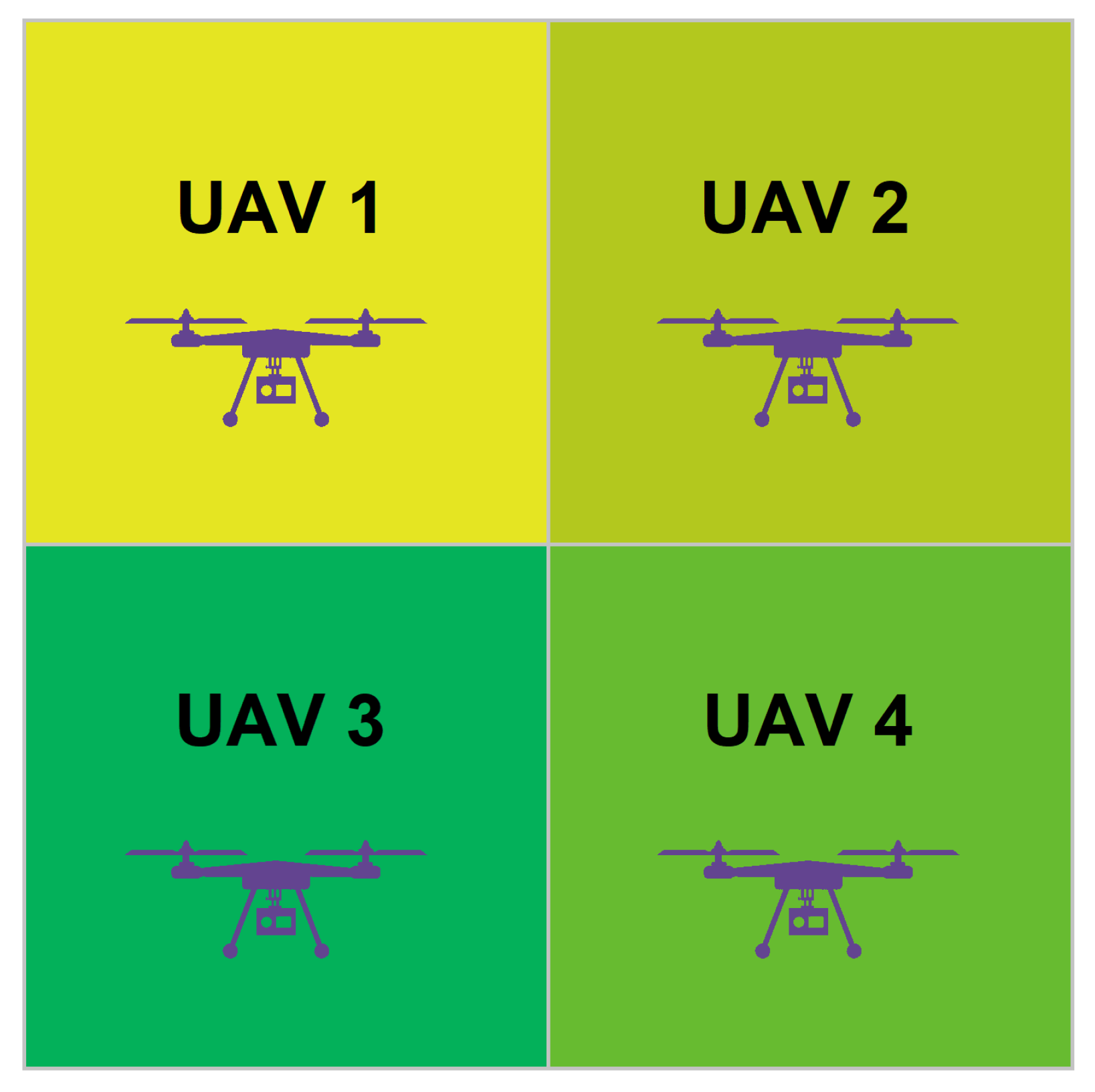
In target detection, UAVs can fly in groups in close cooperation when the targets already exist, and the speed of detection is the first priority instead of the saving cost. This is often the case in military detection or object destruction. Many researchers have focused on the study of UAV cooperation during known target detection. However, for forest fire detection, one UAV often surveils a particular area of land since the possibility of a forest fire is much lower compared with a known target. Sending too many UAVs will increase the cost dramatically and is not necessary. Reducing the cost is the first priority instead of the speed of detection in forest fire detection. For example, for a small area of land, the area can be divided into four parts, as shown in
Figure 1. Each part is dispatched with a UAV. They work independently in their respective areas and do not cooperate with each other. Many papers on UAV forest fire detection treat UAVs as independent individuals. The real-world factors that affect UAVs are wind, rain, and snow. In rainy or snowy weather, UAVs are not often used, since water or snow may cause mechanical and electrical damage to the machine. The only remaining factor is wind. We performed the simulation under different deviations of wind speed. Additionally, we treated the wind as a three-dimensional vector instead of a scalar. In
Section 3, the experiment environment is very close to real-world settings.
When the bat initially searches for prey, it emits ultrasonic waves with a high sound wave volume and a low sound wave frequency, so that it can find out in which small area of the whole environment the prey exists, and then reduce the sound wave volume. It then increases the frequency of the sound waves, searches further in this small area, and finds the prey accurately. Using the bat algorithm to plan the UAV’s trajectory can approximate the UAV as a bat, allowing the UAV to simulate the process of bats looking for prey and avoiding obstacles during flight. In this process, idealized rules can be set as follows. First, the bat perceives the location of the obstacles and target points through echolocation to distinguish the obstacles and target points. Then, the bat flies at the position
at the speed of
, where
and
are three-dimensional vectors. The minimum frequency is
fmin, and the wavelength and pulse volume can be adjusted. At the same time, the bat can autonomously adjust the sound wave frequency according to the position of the bat itself, the obstacles, and the target point. Assuming that the impulse frequency changes from the maximum
fmax to the minimum
fmin, the change interval is related to the real-time problem. The specific rules of the bat algorithm can be described as a multi-dimensional search area to obtain the optimal solution through continuous iterations. In the iterative process, the position
and velocity
of the
n-th generation bat are updated according to the rules described as follows:
where
f[
n] represents the sound frequency at
n-th iteration;
fmin and
fmax are the minimum and the maximum for the initial setting of the frequency;
K[
n] is a uniformly distributed random variable in the range of [0, 1];
and
are the individual position before and after the update, and the update function is given in (4);
is the current optimal solution; and
tg is the quantized time of each step. When the bat finds the approximate range of its prey, it indicates that the local optimal strategy can be used to find the global optimal solution near the current optimal individual as
where
u1[
n] ∈ U(−1, 1),
αx[
n],
αy[
n], and
αz[
n] are the volumes of the sound wave in the
x,
y, and
z directions, respectively. The search can be carried out in a local range. The rules for the adjustment of the volumes
αx[
n],
αy[
n], and
αz[
n] and the pulse indicator
r[
n] can be described as
where
β is the wave propagation constant and
u2 ∈ U(0, 1). When the iteration is close to infinity, the pulse indicator gets closer to
r[0].
It can be observed from Formulas (1) to (6) that this algorithm is sensitive to four major parameters. If u2 is too small, the algorithm converges too quickly, which leads to premature problems, and the obtained solution is not optimal. If u2 is too large, the search time increases and the search result is close to the optimal solution, but the algorithm’s calculation time becomes longer. If β is large, the current position of the bat is updated according to the formula. Otherwise, the search continues near the current optimal position. Since it is affected by the current optimal position, the search easily falls into the local optimal position. Therefore, together, u2 and β determine the search accuracy and convergence speed of the bat algorithm. The search process of the bat algorithm includes a global search and a local search. Although it has a good global optimization performance, it also easily falls into local optimization, which greatly affects its convergence speed and accuracy.
During the flight path, the UAVs are required to find a path from the starting point to the end point with certain constraints. In [
77], the consumption cost is the energy that is consumed to keep the UAV at certain height. Then, the target function can be given as
where
γ is a positive scaling factor. Since it is different for UAVs that move in the
xy directions and the
z direction, we modified the distance function as
where
k is the coefficient to characterize the extra efforts when the UAV moves in the
z direction. (
xs[
n],
ys[
n],
zs[
n]) and (
xe[
n],
ye[
n],
ze[
n]) are the coordinates of the starting point and ending point, respectively. The target function employed is the Euclidian distance function, which can be expressed as follows:
Due to the small number of parameters and the cooperation mechanism, the bat algorithm has strong flexibility and is easy to combine with other technologies so as to improve the performance of the original algorithm and, at the same time, solve complex continuous optimization problems and discrete optimization problems, which shows that the bat algorithm has a wide applicability. The framework of the bat algorithm is as follows. The first step is to initialize the parameters of the algorithm, that is, the population of the bats, the iteration number, the target function, the positions of the bats, the flying speed, the frequency, and the volume. Then, through iteration, the optimum positions of the bats are selected. Additionally, the velocities of the bats are updated. A random number with Gaussian distribution u1 is generated at this point. If u1 > r[n], then a global search is performed to select the bat in the optimum position at the given search area. If this condition is not satisfied, then the position is updated based on the principle. At this time, a second random number u2 is produced. If u2 < r[n] and the target function is smaller than the threshold fth, then the position is acceptable at this stage, or r[n] should be adjusted. This is the step of one recursive procedure in the whole process. If the convergence condition is reached, then the program stops, and the optimum path can be obtained. If the convergence cannot be achieved at the maximum iteration step Nmax, then the program also stops and produces a path. After many steps of iteration, the optimum solution often cannot be obtained. The algorithm itself also has some unavoidable defects and easily falls into local optimization and low optimization accuracy in the later stage, which affect the search ability of the bat algorithm and restrict the ability and scope of the algorithm to solve forest fire detection problems. The flow of MSC-BA algorithm is shown in Algorithm 1.
| Algorithm 1 The MSC-BA algorithm |
Begin
Initialize fmin, fmax,,, tg, K[0], r[0], Nmax, fth, αx[n], αy[n], αz[n], β
for i = 1:m do
for n = 1:Nmax do
compute frequency form (1)
compute solutions from (2) and (3)
generate u1
if (u1 > r[n]) then
calculate and r[n+1] from (5) and (6)
calculate cost from (7)
produce ft[n] from (9)
generate u2
end if
if (u2 < r[n] and ft[n] < fth) then
accept the current position as the optimal position
end if
end for
end for
End |
Generally, the global optimization method is used to optimize the current bat population, which enhances the local search performance of the bat algorithm. Some improved algorithms are more suitable for solving high-dimensional problems, and some algorithms are only suitable for certain specific problems and assumptions, and cannot effectively solve all optimization problems. Therefore, it is very necessary to continue to improve the existing bat algorithm or propose new improvement methods to solve more optimization problems and management problems, and it also has certain practical significance. Compared with other intelligent algorithms, the BA has many advantages. The algorithm has fewer parameters and a fast convergence. The algorithm also has significant disadvantages. Since the bat algorithm does not have a mutation mechanism in the population, the lack of diversity in the population causes the bats to think that the local optimal solution is the global optimal solution when they find the local optimal solution, so they fall into premature areas. So, the problem for the BA is that the global convergence is based on probability and a strong convergence.
2.2. Improvement of BA through Weighted Variation
The improvement of the bat algorithm itself is mainly achieved by adjusting its own parameters so that the algorithm can jump out of the local optimum. Therefore, the algorithm can solve the problem faster and more accurately. It assumes that the bats are randomly distributed and widely spaced. In practical problems, most bats do not meet this requirement. Second, the locally optimal solution may be missed if the step size is too large. When the algorithm is used for each cycle of the algorithm, it is necessary to judge the gap between the fitness and the optimal solution, which increases the time and complexity of the algorithm.
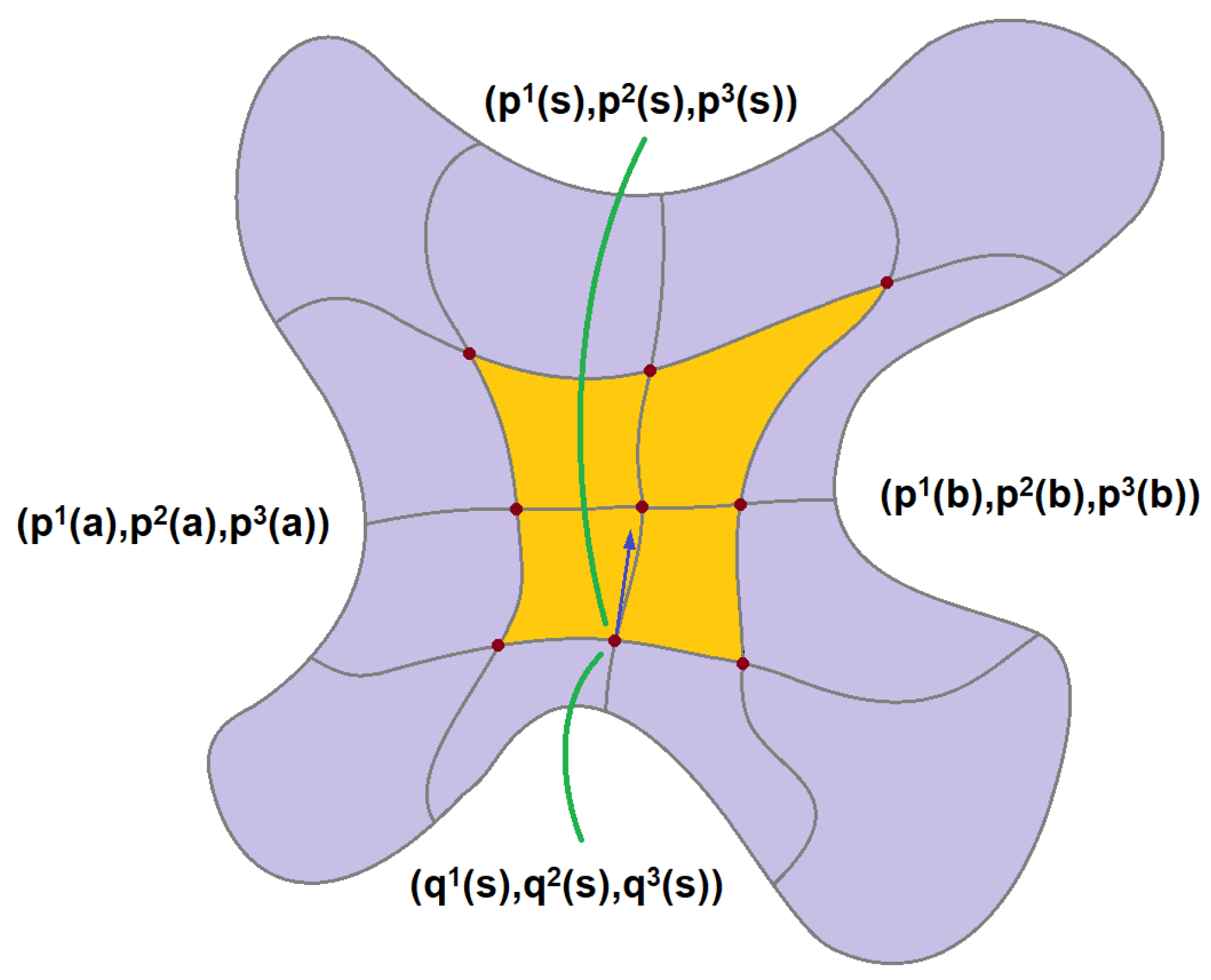
Topological manifold refers to the topological space of the local isomorphism in the Euclidean space, and in general, in order to adapt to the needs, it is often required that this topological space satisfies the separation property and has countable topological bases. This refers to the existence of a neighborhood of any point, which is isomorphic to the Euclidean space. The topological manifold considered here is boundless, and for some marginal manifolds, it is not possible to require that their boundary points have neighborhood homology in the Euclidean space, so in this case, the object of the same morphism will replace the entire Euclidean space with the half space of the Euclidean space. On a curved surface, a geodesic has similar properties. As shown in
Figure 2, the variation of the curve
C is defined above the surface
S, where s is the arc length parameters of the curve
C.
p is the differential function along the curve
C during variation. This can be used to model both concave and convex landscapes. The differential function defined on the area can be given as [
78]
where
s represents the geodesic distance is each direction and
t represents time. The curves of each planning in the variation of the UAVs are dynamic. The initial condition should be satisfied as
This is a variation of the curve
C. It is a continuous function of time and can evolve itself after each step. If the variation has fixed end points, then
For each parameter, the function group provides a curve, and its parameters can be restricted as
It can be shown that the curve
L is a member of this family of curves with the condition of
L =
L0. Therefore, the variation of the curve
C is to embed it in a curve family
Lt that changes around it. This can be seen as the sets of time varying lines in an enclosed sprawling manifold. Outer differential forms can also be defined on differential manifolds. The
p external differential form is a linear combination of the exterior products of some differential that are asymmetrical as
p covariant tensors. It also implicates that the variational curve
Lt of the curve
L and the curve
L have the same starting point and end point. Therefore, curve
Lt is a subset of curve
C. It should be pointed out that although the parameter
s can be assumed to be the arc length parameter of the curve
L,
s is not necessarily the arc length parameter of the variational curve
Lt. Then, the cost of the curve
L can be calculated as
where
Sxyz[
n] is a set of weighted surfaces above the landscape which contains the starting point and the end point. The flight routes of the UAVs are the subspaces of
Sxyz[
n]. During the numerical analysis, the starting surface
Sxyz[0] can be generated as an arbitrary curvilinear plane above the landscape. Through each iteration,
Sxyz[
n] may change after each step. During each step, the cost changes with the evolution of the line sets. If the curve
L has the lowest cost connecting its two end points, its cost should not be larger than the cost of the other curves connecting the end points of the curve
L. In particular, if the curve
L is embedded in any line set that has the same end point, the variational curve family
Lt could satisfy
When the curve
L above the surface
S satisfies this condition with respect to its variational
Lt, the arc length of the curve
L reaches its variational curve
Lt. The external characteristics of the surface
S are only related to the first basic form of the surface
S, which indicates that the above considerations belong to the category of the intrinsic geometry of the surface
S. The partial derivative
q of the curve
L can be expressed as
The partial derivative
q of curve
L is a tangent vector field defined along the curve
L on the surface
S as the variational vector field of the variational. The variational vector is the variational in
s =
s0 and the tangent vector at
t = 0. For the variation of the curve
L with fixed endpoints, its variational vector field at the endpoints is zero. Conversely, if a tangent vector field is given along the curve
L on the surface
S, then a variation of the curve
L can be defined with the variational vector field as
The first basic form of the surface
S is
where the function
Sxyz[
n] is the first fundamental form of the surface
S from differential geometry in the
n-th step. Then, the cost of the variational curve
Lt is
The specific process of using the AWVM-BA is described as follows. First, the appropriate fitness function is selected, and the relevant parameters of the algorithm are initialized, including the population size, the scaling factor, and the probability of crossing. Then, a population is randomly generated based on the initial parameters. Then, the fitness function of each individual in the current population is calculated. At this stage, it is determined whether the algorithm can be terminated at the present time. If it can be terminated, the result can be output; otherwise, the algorithm continues to run. Mutation and crossover operations are performed to create new individuals. In the mutation operation, the difference between the two individuals is multiplied by the scaling factor and added to the third individual to obtain a new individual. In the crossover operation, a hybridization probability is set. If the conditions are met, a new individual is created according to the hybridization probability. Then, the selection operation is performed to select individuals from the current population and create a new population. Finally, the number of iterations is increased by one, and the execution continues with the previous steps.
2.3. Other Improvements and Modifications of the Proposed AWVM-BA
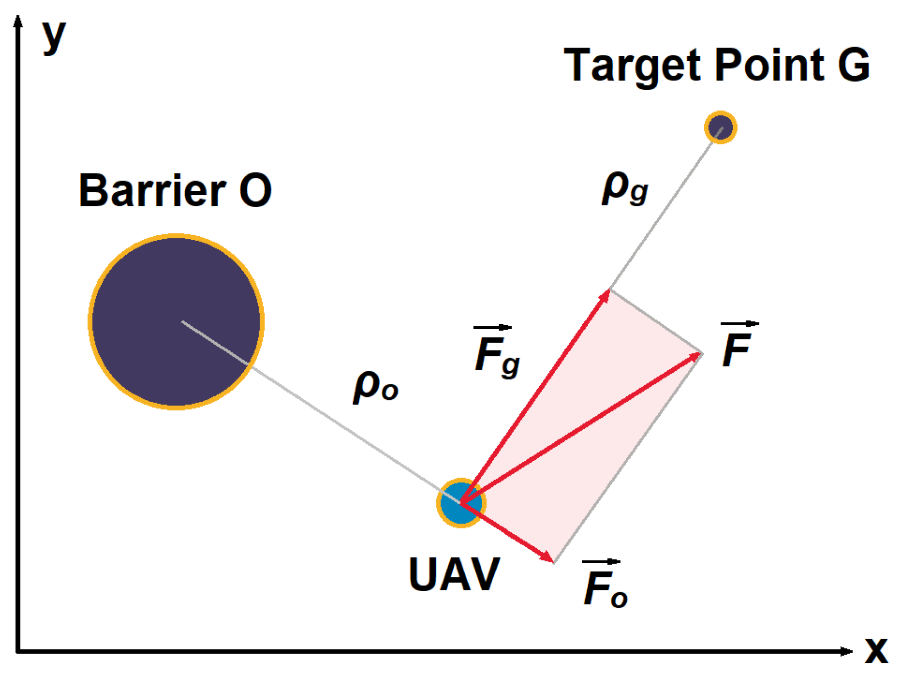
The improved artificial potential field method (APF) can be carried out to analyze the force exerted on the UAV [
79], as shown in
Figure 3.
and
stand for the attractive force and repulsive force, respectively.
ρo represents the distance to the barrier and
ρg represents the distance to the target point. First, the attractive potential
UG[
n] and the repulsive potential
Uo[
n] can be given as
where
ε is defined as the scale factor.
dgoal is the threshold for the distance between the UAV and the target point and
dob is the threshold for the distance between the UAV and the barrier. Then, in combination with the variation method, the cost can be modified as
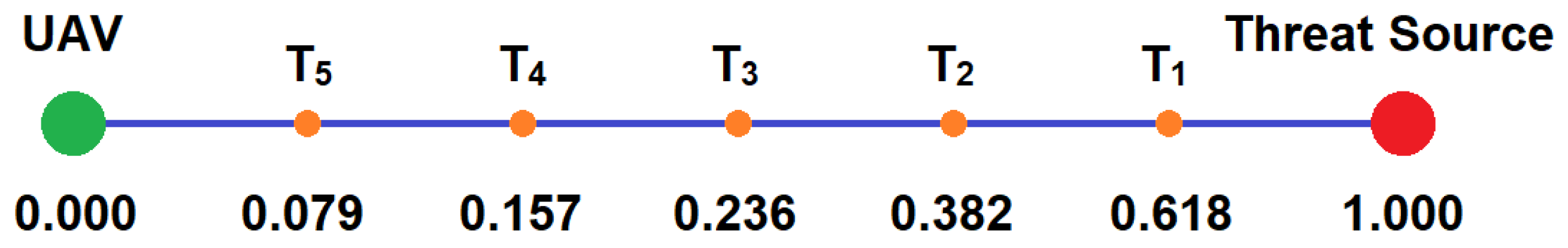
The mountain peaks in the forest that are higher than the flight range of the drone can be considered as obstacles. The flight path of the drone for firefighting should be planned in an obstacle environment. The distance between the obstacle and the drone is divided into six parts, and five points are selected in the flight path, namely, points
T1,
T2,
T3,
T4, and
T5. When flying on this trajectory, the threat at each division point is different, as shown in Formula (25). The threat from the obstacles at the site is shown in
Figure 4. The designed division is based on the mathematical golden ratio, which can avoid threat at the optimal distance.
Then, by considering the threat cost value, the final variational cost function can be modified as
2.4. The Implementation of the Proposed AWVM-BA
The implementation steps of the hybrid bat algorithm based on differential evolutions are as follows. First, the algorithm parameters and population size are initialized. In the forest fire area, an initial trajectory from the starting point to the fire location is randomly generated with the initial solution. Next, the algorithm parameters, the size of the population, the initial position, the speed of each bat, the sound wave frequency, and the sound wave loudness of each bat are set. Then, each individual is evaluated, and the best individual in the population is selected at the moment. For each track point at the initial moment, the distance between each track point and the threat of obstacles in the environment to the current track point are calculated. The fitness value is obtained with the minimum track point of the function value. Next, the speed and position of the individual bat are updated. Each track point is renewed. After that, a local disturbance operation is performed on the current optimal bat individual. Additionally, the location of the local solution is used to replace the current optimal solution. The track point with the best fitness value in the track then is offset to a certain extent. This operation is mainly used to prevent the track generated by the algorithm from being the local optimal one. Otherwise, no offset is performed with respect to the operation of the track points. The next step is to accept the renewed solution. If the previous condition is satisfied, then the new solution is accepted, and the loudness of the sound wave is then updated. At this point, the global optimal solution is updated. The obtained bat populations are sorted to find the position of the optimal population. The next step is to determine whether the algorithm is iteratively terminated or whether the algorithm has reached the maximum number of iterations. If the maximum number is reached, the algorithm execution is terminated. Otherwise, the algorithm returns to the previous steps, and the iteration continues. The final step is to output the optimal solution of the UAV to perform the task.
The differential evolution uses a differential strategy for individual mutation. Its idea is to sum the difference between the current individual and two randomly selected individuals in the population to obtain a new individual as
where
F is the logistic factor that decides the position variable
x[
n] between each time step. If
F is below 4, the
x increases at a linear step without random distribution between each step. When
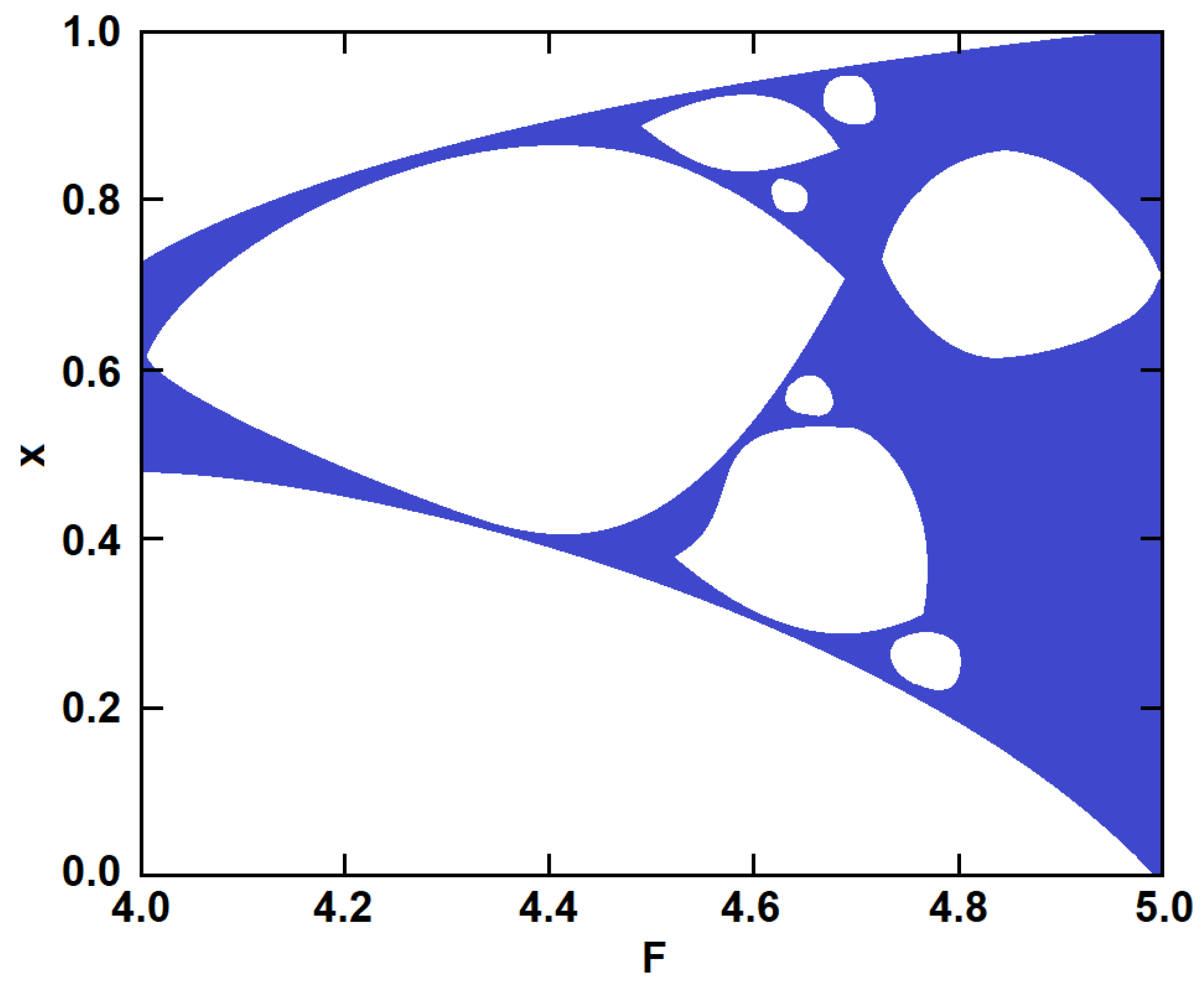
F reaches above 4 and below 5, the distribution changes at large intervals with the property of gradual randomness. We performed the logistic mapping, and the results are shown in
Figure 5. In the case where
F reaches 5, the distribution is in the full range between 0 and 1. Then, in the solution space, the proposed algorithm can avoid the local minimum with an enhanced solving speed using this chaos strategy, which is also integrated in our proposed algorithm. The drawback of the proposed algorithm is that the amount of computation can increase faster with the complication of the outside environment, such as the deviation of wind speed. Additionally, it is shown in the final experiment that the iteration number of the proposed algorithm increases faster compared with some other intelligent algorithms. This is the main disadvantage of the proposed AWVM-BA. The flow of the proposed algorithm is given in Algorithm 2.
| Algorithm 2 The proposed bat algorithm using asymmetrical variational method |
Begin
Initialize fmin, fmax,,, tg, K[0], r[0], Nmax, fth, F, x[0], Sxyz[0], β, k1, k2
for i = 1:m do
for n = 1:Nmax do
compute frequency form (1)
compute solutions from (2) and (3)
calculate the path variation cost from (26)
calculate individual mutation from (27)
generate
if () then
accept the current cost as the minimum
end if
calculate and r[n + 1] from (5) and (6)
produce ft[n] from (9)
if (x[n] < r[n] and ft[n] < fth) then
accept the current position as the optimal position
end if
end for
end for
End |
3. Calculation and Simulation
Several algorithms are compared using the simulation experiment to test the optimization performance of the proposed improved bat algorithm in different environments. The simulation is performed through programming. In this experiment, the size of the bat population is set to 70, and the maximum number of iterations of the algorithm is 50. In the optimal solution update formula, the update cost is set to 0.5, and the maximum threat cost of obstacles is 0.9. The differential evolution algorithm is used. When performing the bat population mutation, the scaling factor of the differential evolution algorithm is set to 0.7. The size of the simulation environment is 1 km × 1 km, including the horizontal and vertical coordinates of the center point of the obstacle and the obstacle radius, as shown in
Table 1. The obstacles are expanded, and the radius of the obstacles is increased by 2 m to ensure safety during the flight. The maximum allowed flight height is set at 120 m to ensure flight safety.
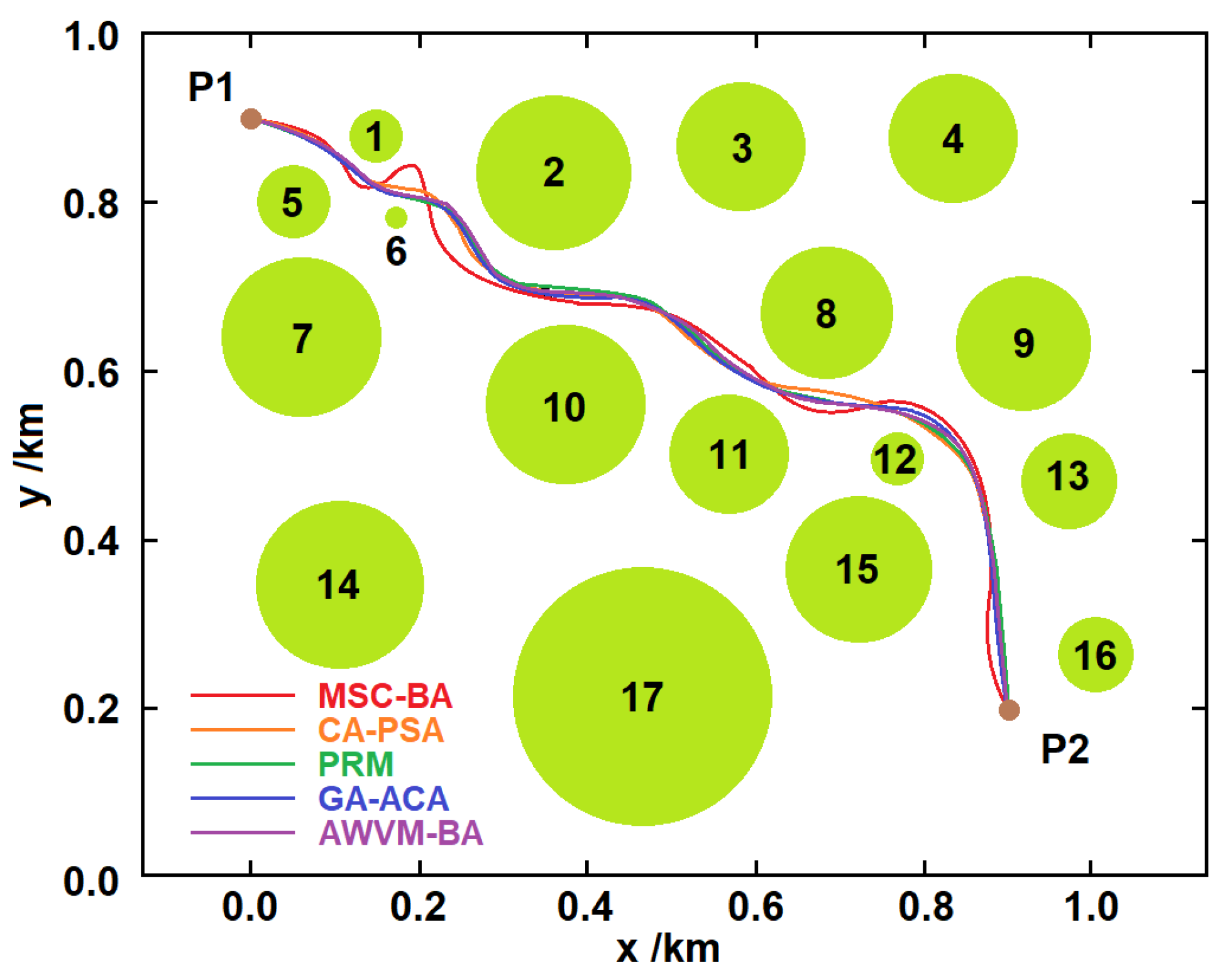
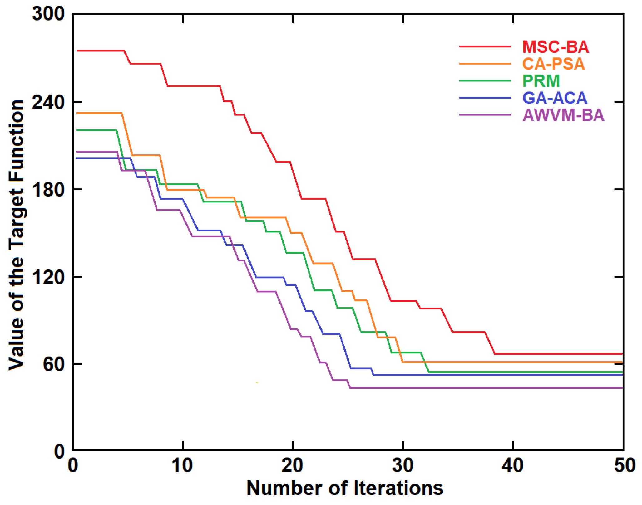
In this obstacle environment, the AWVM-BA algorithm and some other algorithms are used for simulation experiments. The simulation results are shown in
Figure 6 and
Figure 7. In
Figure 6, the UAV is designed to fly from P1 to P2 with 17 obstacles in the region. These obstacles are denoted as green circles where the UAV should not be able to fly across.
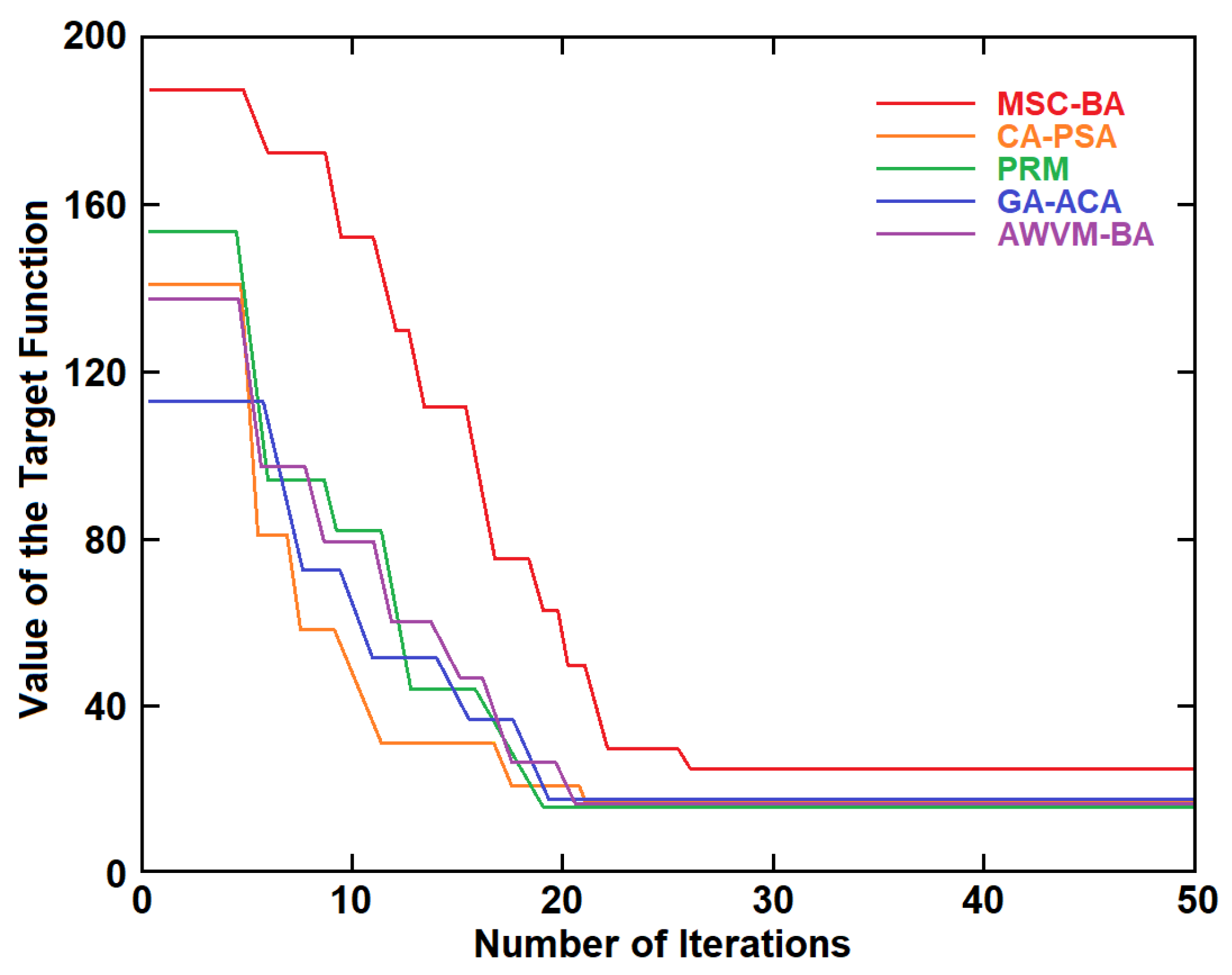
Figure 7 shows the convergence curves of the algorithms. The slope of the convergence curve represents the convergence speed of the corresponding algorithm. It can be seen that the PRM has the best convergence performance in the convex obstacle region. Through continuous iterations, the flight target function of the UAV has a relatively fixed value in the convergence range, which can be used to monitor the convergence accuracy of the corresponding algorithm. The fitness function is the threat of the obstacle to the UAV. The data in
Table 1 are evaluation indicators for different algorithms for trajectory planning. By combining the simulation results and the trajectory evaluation indicators, it can be concluded that the proposed AWVM-BA shows comparable performances to some other recently proposed algorithms.
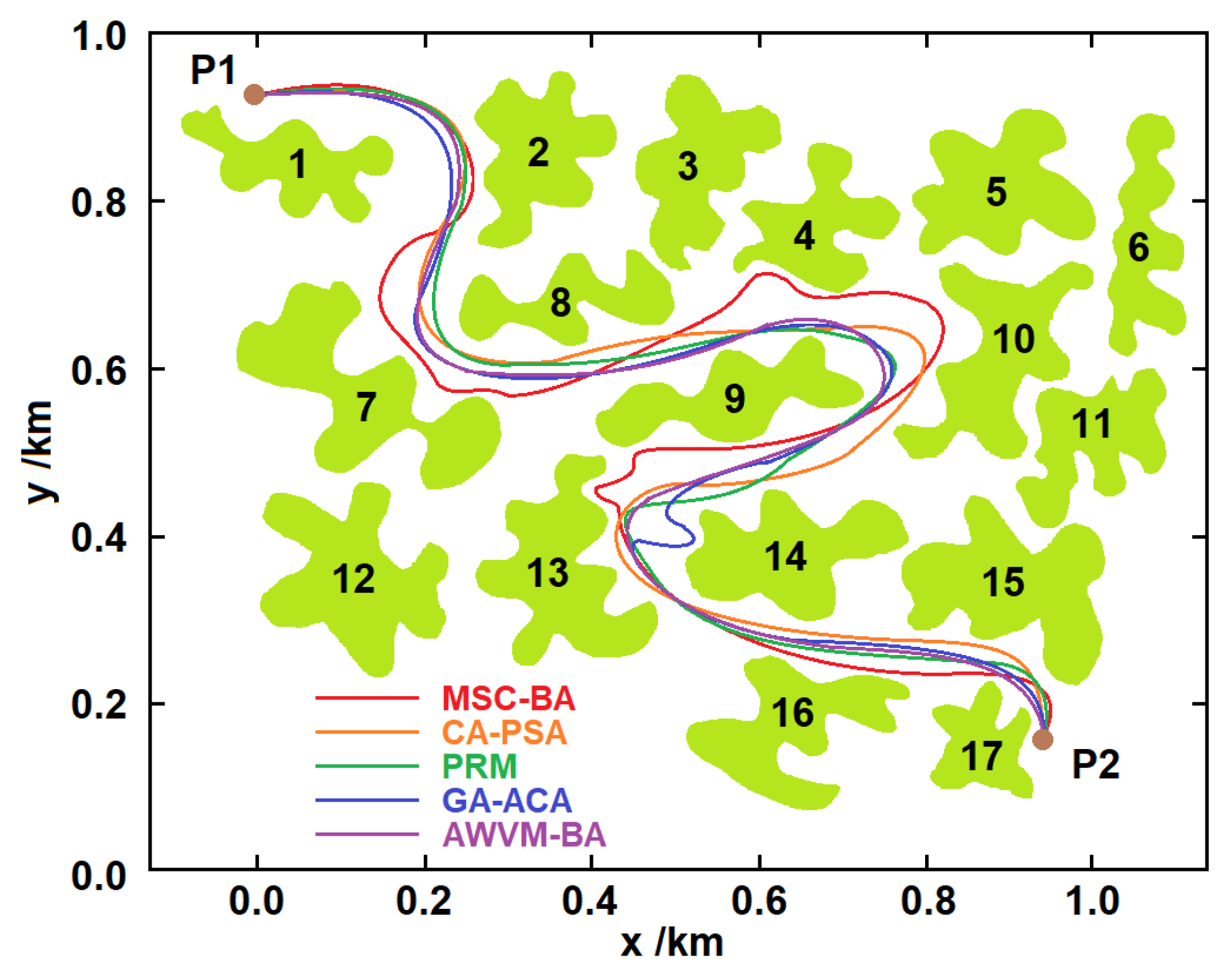
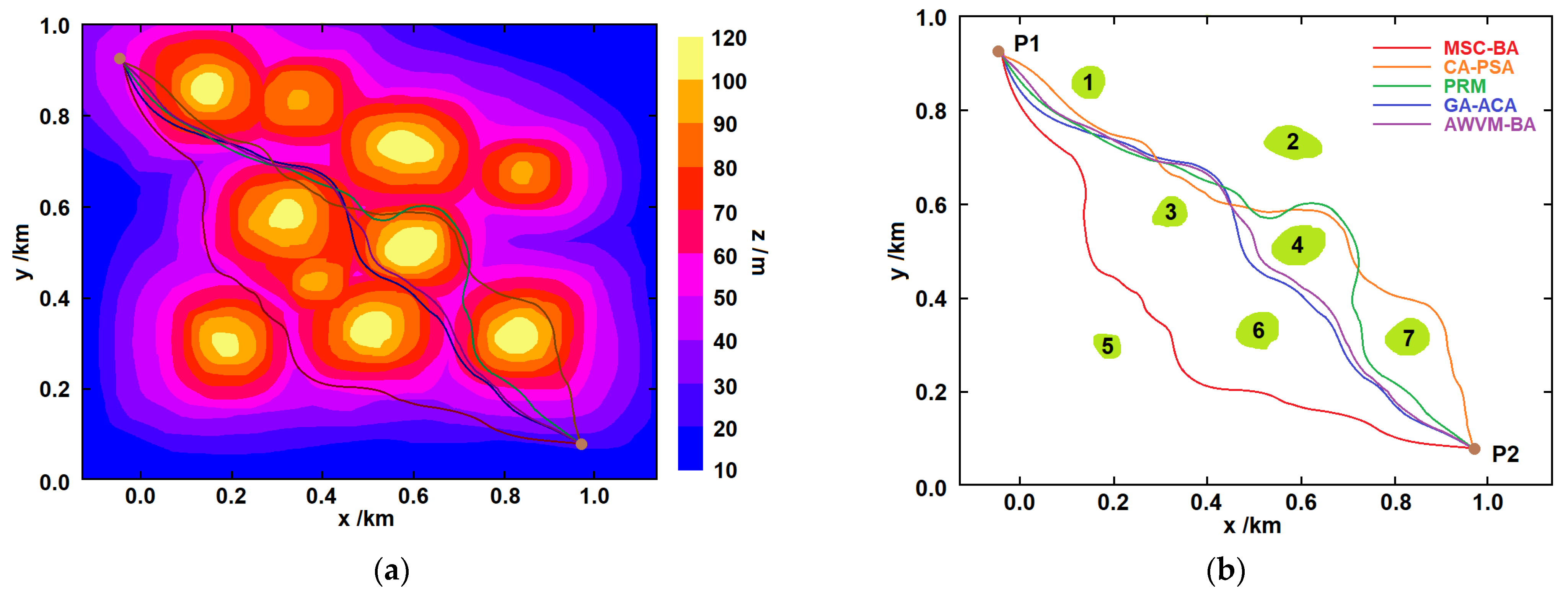
Since the obstacles are round and convex, it saves the trouble of local optimization and expedites the convergence speed. In the next experiment, we changed the obstacles with rugged outlines. Additionally, in this environment, we compared the performances of the AWVM-BA algorithm with some other algorithms. The results are shown in
Figure 8 and
Figure 9. It can be seen that the AWVM-BA has the best convergence performance in the convex obstacle region, with the shortest path length and the lowest cost. Through continuous iterations, the flight target function of the UAV is relatively fixed in the convergence range, which can be used to monitor the convergence accuracy of the corresponding algorithm. For the concave surfaces, the reflected detection parameter can easily focus on a local optimum just as a ray of light being reflected by a concave mirror to form a focus point. With the increase in the iteration, the situation is unbalanced by the free parameters in the algorithm. This process can be regarded as changing the curvature of the mirror. Then, the planned path from P1 to P2 is renewed after each iteration. The target function does not always decrease with the increase in the iteration number for some algorithms. In our experiment, we chose some recent intelligent algorithms for performance comparison. They are stable and converge fast without irregularities during iterations. So, the target function decreases with each iteration. The data in
Table 2 are evaluation indicators for different algorithms for trajectory planning. The concave parts along the obstacles can lure algorithms into local optimization more easily. By combining the simulation results and the trajectory evaluation indicators, it can be concluded that the proposed AWVM-BA shows the best performance.
The influence of uncertain factors can easily lead to the inaccurate execution of firefighting tasks. When the drone’s flying altitude is too low, there is a large number of obstacles, such as mountains and trees in the environment, and flames will also cause safety issues to the drone itself. Therefore, the flying height of the drone cannot be too low or too high, and the flying height should be adjusted at any time along with the ups and downs of the undulating mountains in the environment. The drone’s flight should consider the altitude of the current flight position at this time, and then the drone can be on the further planned trajectory in the forest firefighting mission.
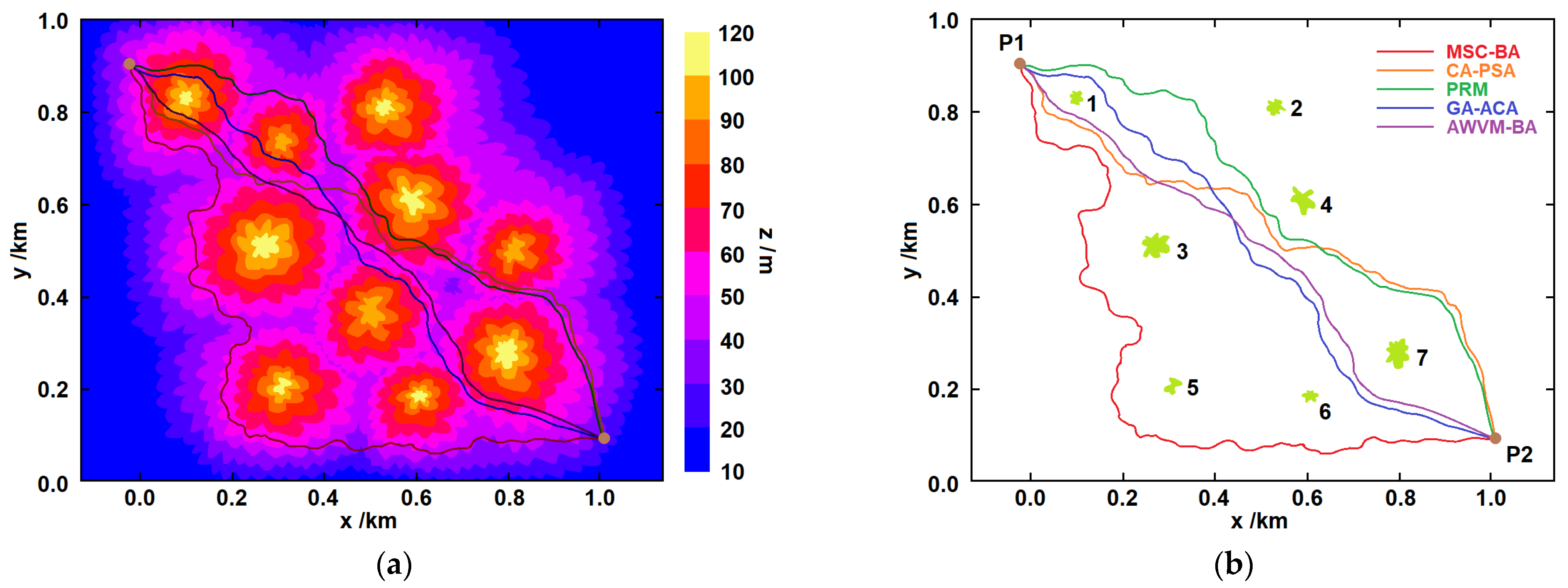
The AWVM-BA algorithm, with some other newly proposed algorithms, are simulated in a continuous gradient environment for the trajectory planning. The size of the task space is 1 km × 1 km, as shown in
Figure 10. In order to ensure the safe flight of the UAV, the obstacles are expanded, and the radius of the obstacles is increased by 1 m.
The simulation results are simulated in circular convex regions with a continuous gradient. The results show that these algorithms can plan a safe flight path for UAVs in mountainous areas, meeting the requirements of UAVs for firefighting in mountainous areas, and proving that the algorithms are feasible and correct.
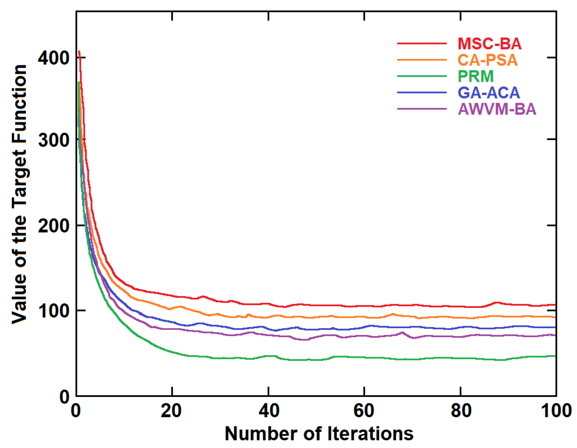
Figure 11 shows the change curve of the target function value that the algorithm runs when used for trajectory planning. Through the comparison of the iterative curves, it can be seen that the target function value of the trajectory planning is better for the PRM algorithm. Still, the AWVM-BA shows relatively comparable results with the other algorithms. The smaller the obstacles threatened by the drone during the flight are, the safer the planned trajectory becomes. The data in
Table 3 are the evaluation comparison of the five different algorithms for trajectory planning. By combining the simulation results and the trajectory evaluation indicators, it can be concluded that the UAV trajectory planned by the AWVM-BA has a shorter length and poses a smaller cost to the UAV. It is also more conducive to the UAV flight.
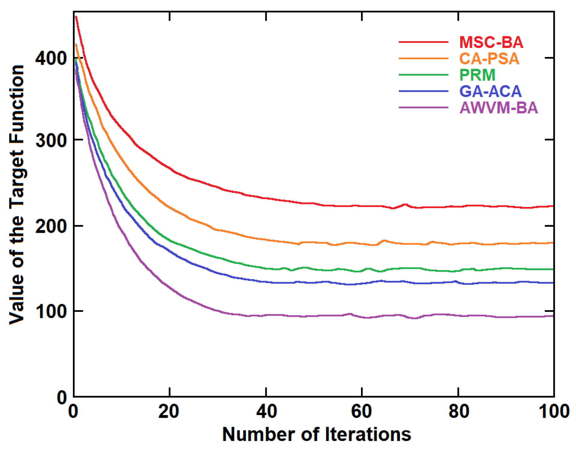
Next, we simulated the results in concave regions with a continuous gradient, which are shown in
Figure 12. These results also show that these algorithms can plan a safe flight path for UAVs in mountainous areas, meeting the requirements of UAVs for firefighting in mountainous areas, and proving that the algorithms are feasible and correct in concave regions with a continuous gradient.
Figure 13 shows the change curve of the target function value that the algorithm runs when used for trajectory planning. By comparison, the target function value of the trajectory planning is better when the bat algorithm is based on differential evolution. The data in
Table 4 give the performance comparison of the five different algorithms in concave regions with a continuous gradient. By combining the simulation results and the trajectory evaluation indicators, it can be concluded that the UAV trajectory planned by the AWVM-BA has a shorter length and a smaller cost to the UAV compared with the other four algorithms.
In the actual flight route planning, it is necessary to consider the wind condition from the viewpoint of fuel consumption. Additionally, it is necessary to consider that the fire area also expands and changes depending on the wind conditions. Since the wind speed is not a known variable in a local region, we modeled the wind behavior as a three-dimensional continuous Brownian stochastic process. Due to the effects of the landscapes, the wind moving in the
xy direction is much stronger than that moving in the
z direction. Therefore, we introduced a damping factor
Dp.
Dp is in the range of [0, 1]. If
Dp is 0, then there is no wind flow in the
z direction. Additionally, if
Dp is 1, then the strength of the wind flow in the vertical direction is the same as that in the horizontal direction. Therefore, the wind behavior can be modeled as
where
,
, and
are the three basic unit vectors in the
xyz coordinate systems. The components
Bx,
By, and
Bz are independent to each other. In general conditions, the probability of wind directions is equally likely. Therefore, we took the expectation of each component
μ to be zero. The standard variance
σ characterizes the disturbance and deviation of the strength of the wind with respect to time. If
σ is small, then the wind level is relatively weak around the expectation. However, with the increase in
σ, the wind strength can become stronger during the Brownian stochastic process. As for the special condition, if
σ = 0, this means that the UAVs are flying in the ideal windless environment.
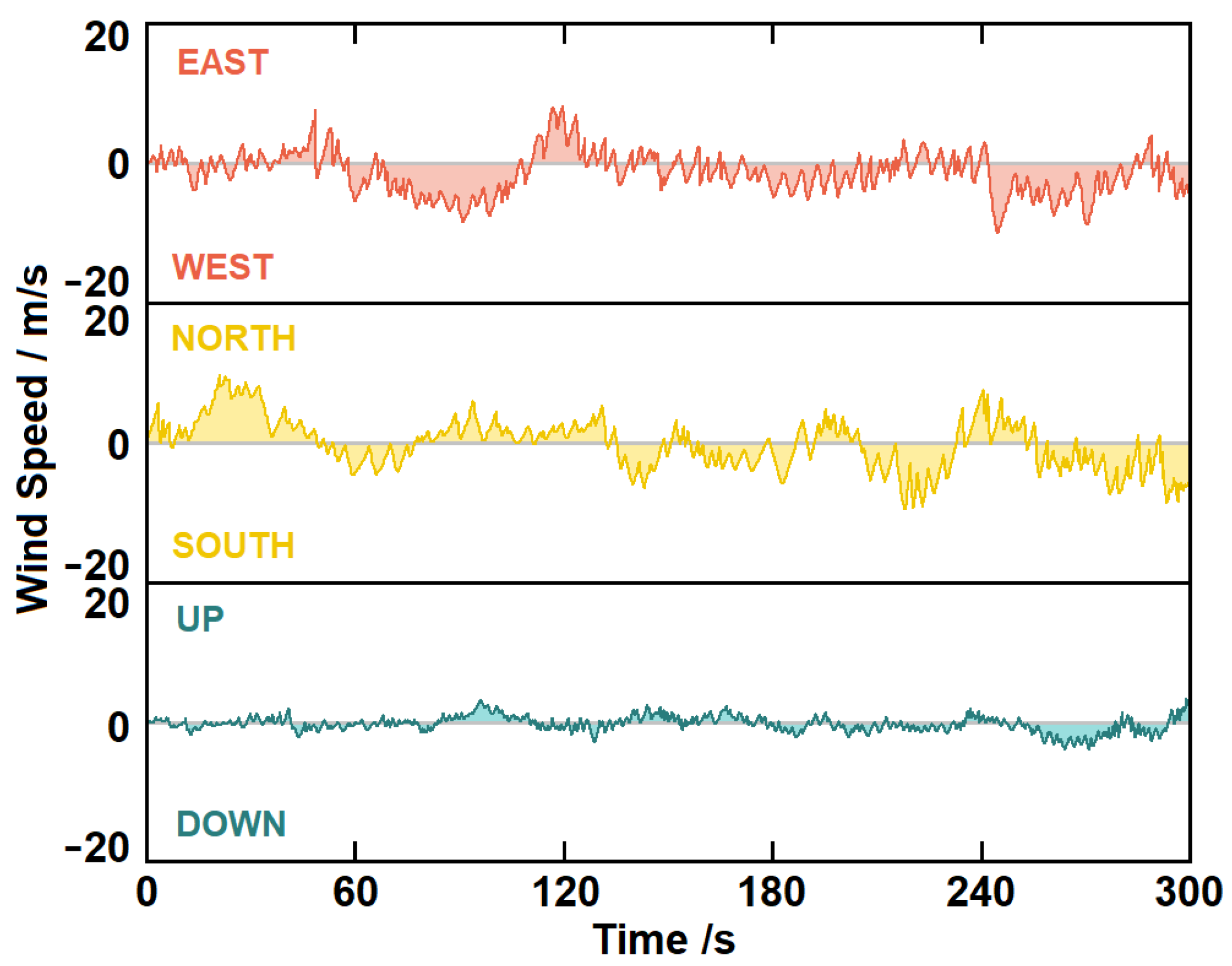
Figure 14 shows the wind speed with respect to time in the
xyz directions as a continuous Brownian stochastic process at the condition of
μ = 0,
σ = 5, and
Dp = 0.2. The deviation in the
z direction is much smaller in amplitude due to the damping factor. If the wind speed takes a negative sign, it means the wind is blowing in the opposite direction. The wind effect can have some influences on the evaluation parameters, such as the flight length, iteration number, flight cost, and TFV. Then, the wind effects can be regarded as the added random noise in the flight of the UAVs.
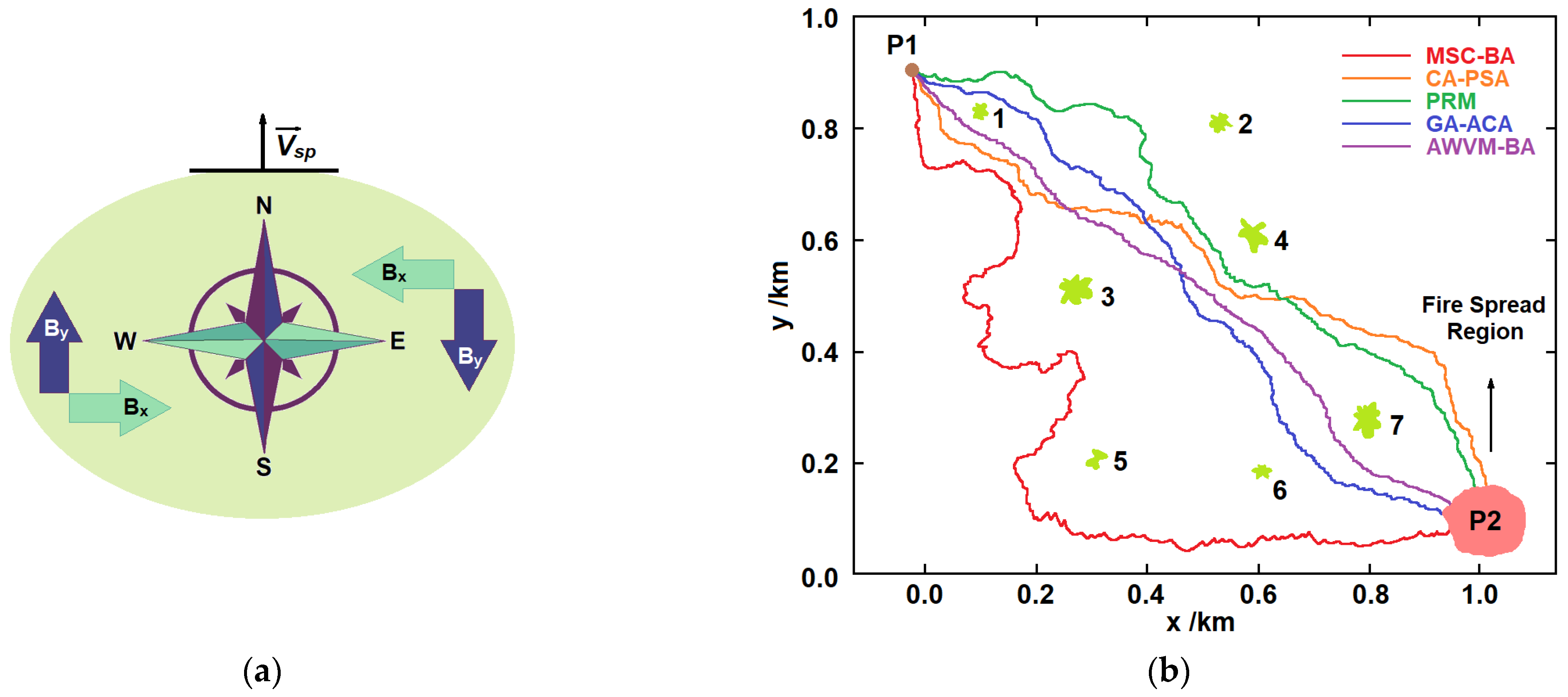
Additionally, it is necessary to consider that the fire area also expands and changes depending on the wind conditions, as shown in
Figure 15a. In a windless condition, the fire spread speed
is determined by the contour of its geometric topology, and can be modeled as
where
is the del operator, and
G(
x,
y,
z) is the contour of the fire region.
kp is the fire spread factor and is affected by the types of plants in the area, since the wind affects the fire spread in the
xy direction. Therefore, if the wind effect is taken into consideration, then the modified fire spread speed can be given as
where
kw is defined as the wind effect factor.
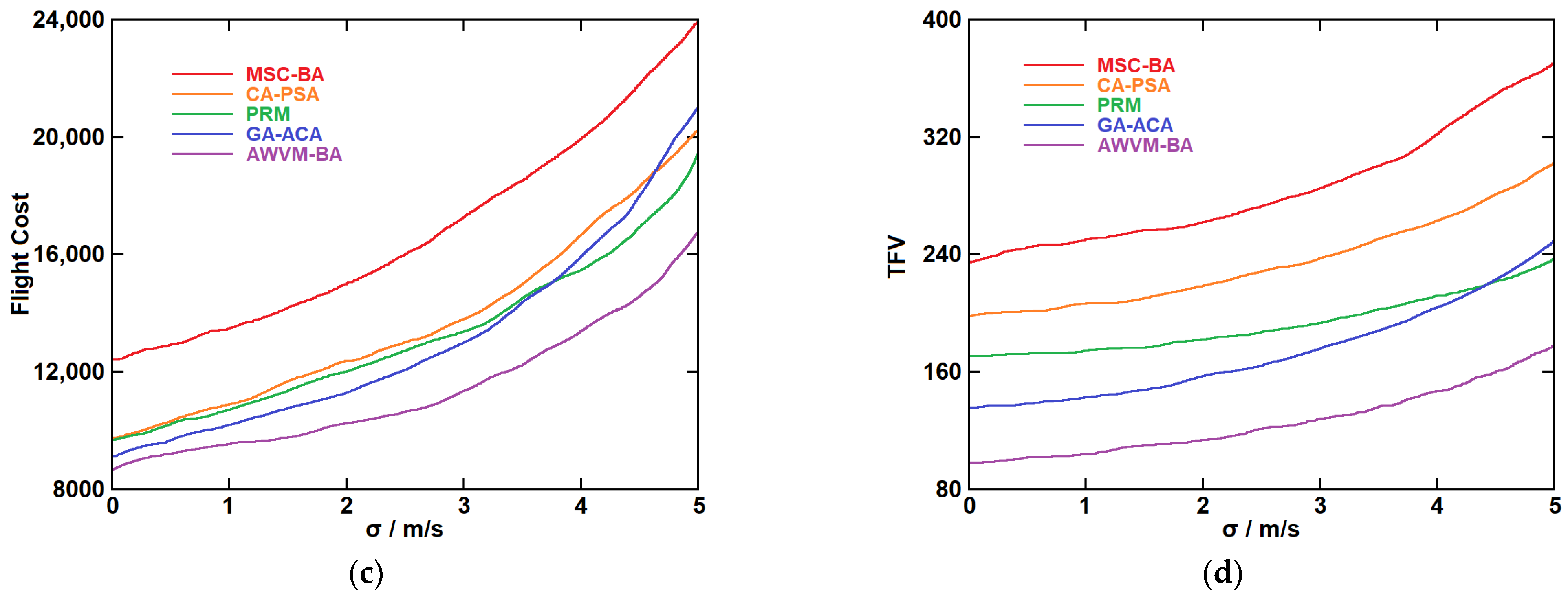
Figure 15b shows the flight path of a UAV under different route planning algorithms with the effects of wind and fire spread. It can be seen that the flight paths become perturbed compared with those in a windless condition. Additionally, some segments of the paths were slightly altered. P2 stands for the fire spread region. The fire spread effect is not that significant compared with the wind effect since the speed of the fire spread is very small compared with the speed of UAVs. In our simulation, we still considered the fire spread effect in the P2 region. The path deviation is mainly affected by the deviation of the wind speed. The exertion of wind has effects on the performance, especially with the increase in the deviation of the wind speed. The wind can be modeled as an additive noise along the flying path. In our experiment, we used the Monte Carlo method with 10,000 independent trials.
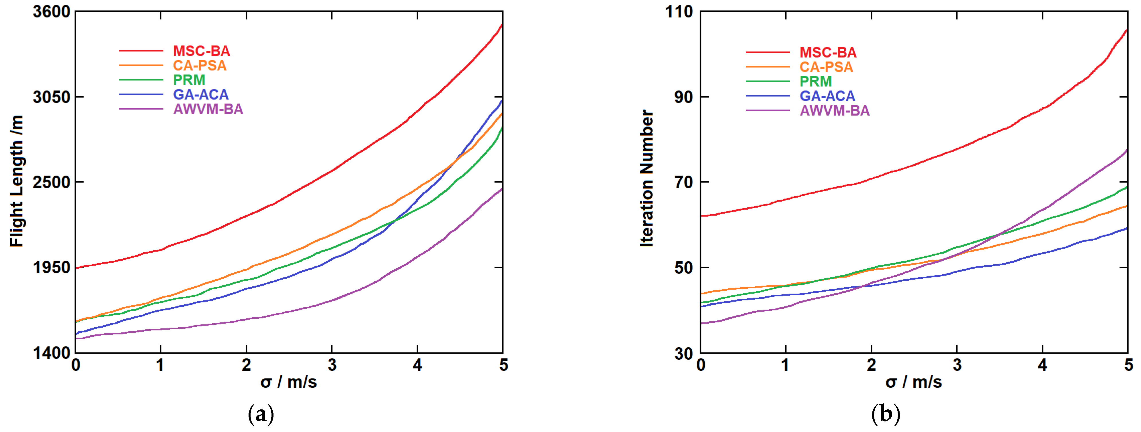
Figure 16 shows the evaluation parameters in consideration of the wind effect and fire spread effect. The proposed AWVM-BA is again tested in comparison with some other recently proposed algorithms. The simulation is based on the Monte Carlo method with 10,000 independent trials. The arithmetic averages were calculated as the final results. It can be seen that the evaluation parameters increase nonlinearly with the increase in
σ. Compared with the MSC-BA, CA-PSA, PRM, and GA-ACA, the proposed algorithm achieved better results in the flight length, flight cost, and TFV. The limitation of the proposed algorithm is that the variation calculation is more sensitive with the added wind effects. Therefore, the iteration number increases more quickly than the other algorithms when
σ increases. This is because the deviation can be regarded as the complication of the sub-dimension surface variation. This can also have an impact on the convergence time. Therefore, a higher calculation ability is required for hardware setup. Still, the proposed algorithm shows a great advantage in convex landscapes in windy conditions.


