Spot–Ladder Selection of Dislocation Patterns in Metal Fatigue

Abstract

Spontaneous pattern formation by a large number of dislocations is commonly observed during the initial stages of metal fatigue under cyclic straining. It was experimentally found that the geometry of the dislocation pattern undergoes a crossover from a 2D spot-scattered pattern to a 1D ladder-shaped pattern as the amplitude of external shear strain increases. However, the physical mechanism that causes the crossover between different dislocation patterns remains unclear. In this study, we theorized a bifurcation diagram that explains the crossover between the two dislocation patterns. The proposed theory is based on a weakly nonlinear stability analysis that considers the mutual interaction of dislocations as a nonlinearity. It was found that the selection rule among the two dislocation patterns, “spotted” and “ladder-shaped”, can be described by inequalities with respect to nonlinearity parameters contained in the governing equations.

1. Introduction

Diffusion usually homogenizes a system. This intuitive idea is consistent with the observation that a drop of ink placed in a glass of water spreads out with time, eventually making the whole body of water cloudy. Surprisingly, however, diffusion can make the system non-homogenous under certain conditions through self-organization of spatial patterns with local or global symmetry. This counterintuitive property is called diffusion-induced instability [1]. The spatial patterns created by this property are called Turing patterns, named after the pioneering individual who first theoretically predicted this phenomenon [2,3].

Turing theory, which explains the spontaneous formation of patterns by diffusion, is based on the following three hypotheses [4]: (i) The system consists of two components: the activator and inhibitor. The former promotes its own local production whereas the latter decelerates its own production. (ii) The two components act to change each other’s local concentration. Specifically, the substrate depletion model [5] was adopted in this work, wherein the activator (inhibitor) is assumed to deplete (enhance) the local growth of the other component. (iii) The inhibitor diffuses over the system sufficiently faster than the activator. Under these assumptions, the local concentration of the activator tends to increase when it is elevated by a small local perturbation; this is true even though the system starts in a homogeneous state. The resulting local maximum of activator population decreases the inhibitor population nearby, causing a downward peak of inhibitor population. As time passes, the width of the inhibitor’s downward peak rapidly broadens, while the narrow width of the activator’s upward peak is maintained, because of the higher (lower) mobility of inhibitor (activator). At this stage, an aggregate of activators forms, which is surrounded by a decreasing inhibitor population within the characteristic length of inhibitor diffusion. Owing to a decrease in local density, the inhibitor cannot promote another aggregate of the activator within a close neighborhood of the first maximum. Nevertheless, when there is sufficient distance, a sufficient population of inhibitors remains so that another aggregate of activators can be formed by following the aforementioned mechanism. By repeating this process, a spatially periodic pattern of the activator aggregate develops [6]. This scenario is based on the premise that diffusion can destabilize a homogeneous state.

Existing studies on diffusion-induced instability have focused primarily on soft matter, including biological [7,8,9,10,11] and chemical [7,12,13,14,15] systems, in which the typical periodicity in length ranges from cm to mm or slightly less. Conversely, Turing patterns that emerge in “hard” matter show far smaller length scales [16,17,18,19]. A well-known example of such Turing patterns in hard matter is the dislocation patterning that occurs inside plastically deformed metal [20,21]. Dislocations are linear-shaped crystalline defects, and are responsible for the mechanical strength and plastic deformation of crystalline materials [22,23,24]. Dislocations are uniformly distributed inside the metal in a pristine state; however, when the metal sample is repeatedly loaded, diffusive motion of individual dislocations followed by reactions that occur between them results in the spontaneous formation of dislocation patterns [25]. These patterns are composed of dense aggregates of dislocation multipoles separated by relatively dislocation-poor regions. In particular, in face-centered cubic (fcc) metals (e.g., Cu, Ni, and Ag), an increase in the amplitude of plastic shear strain during cyclic loading experiments leads to successive transitions in pattern morphology, from two-dimensional (2D) spotted or vein structures at low strains (see Figure 1a,b) and one-dimensional (1D) ladder structures at medium strain (Figure 1c) to more complex structures at higher values. However, the physical mechanism of switching across different patterns has not yet been fully elucidated, despite considerable efforts in the past [26].

In the present study, the production–annihilation rate equation which theoretically reproduces crossover across spot- and ladder-pattern formations in correlated dislocation systems was formulated. In the formulation, the atomic-scale discrete distribution of dislocations was replaced by a continuous distribution of dislocation density. Under the continuum approximation, the nonlinear parameters describing mutual interaction between nearby dislocations were deduced from a few physically plausible assumptions. An approximate analysis based on nonlinear rate equations led to the following conclusion: the threshold for crossover from the 2D spotted pattern to the 1D ladder pattern can be expressed by a combination of the nonlinear terms defined in the formulation. The qualitative consistency of the theoretical results with experimental observations supported the validity of our rate equation approach for the formation of dislocation patterns.

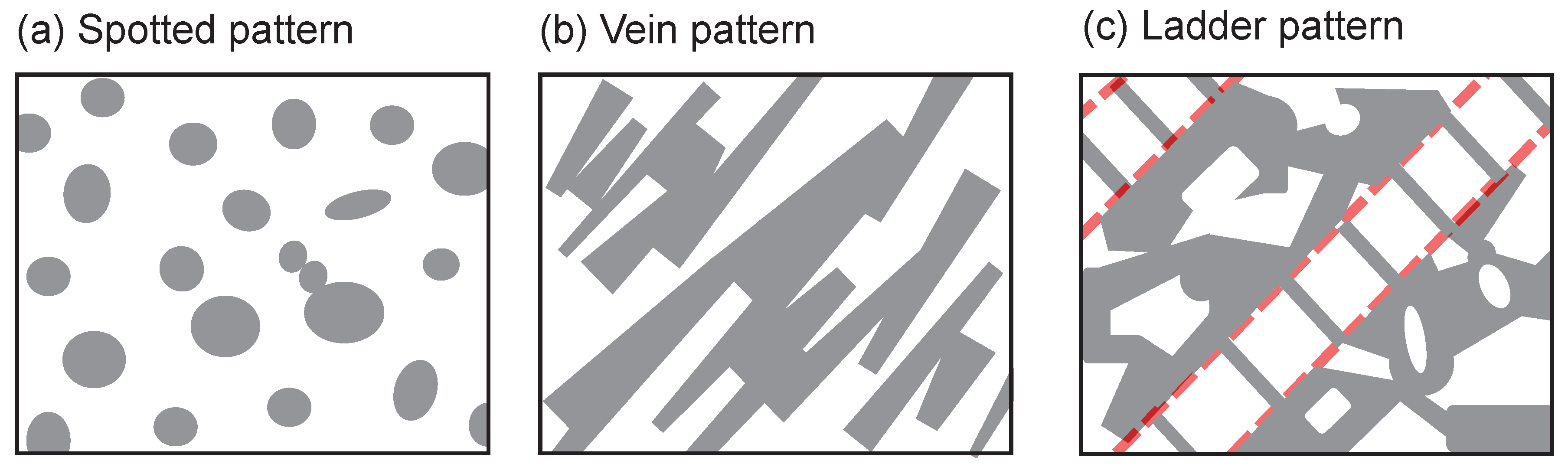
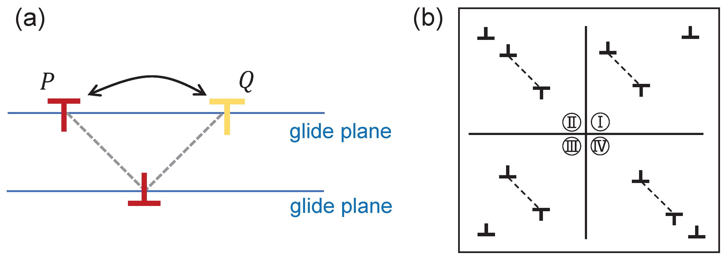
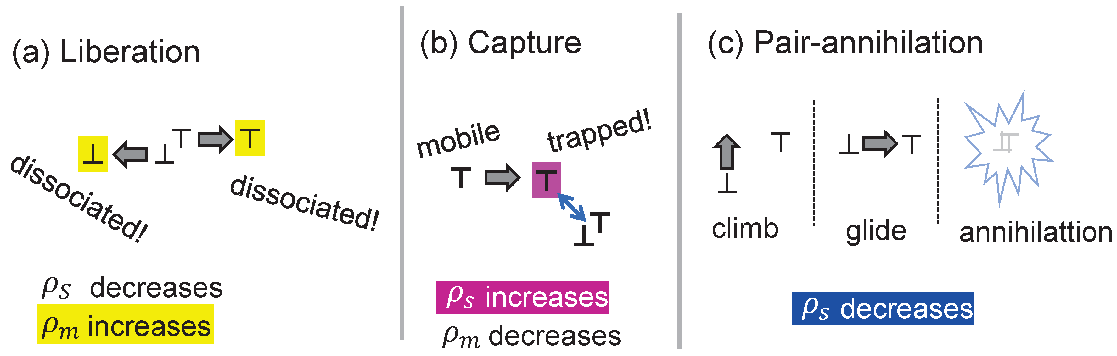
2. Dislocation Patterning and Its Microscopic View

We begin with a brief summary of the initial process of metal fatigue that gives rise to the spontaneous formation of dislocation patterns.

Suppose that a well-annealed single-crystalline metal oriented for a single slip is fatigued in a push–pull cyclic loading experiment [27]. The experiment is conducted by controlling the amplitude of resolved plastic shear strain, maintained at a given constant, (see ref. [20] for precise definitions of terminology). During the first few cycles, the system exhibits work hardening (i.e., a rapid increase in the flow stress with an increasing number of cycles), which is a hallmark characteristic of plastic deformation. With continued cyclic loading, the increment in hardening per cycle gradually decreases and a quasi-steady state of deformation (i.e., saturation) is achieved [28]. Once saturation occurs, the variation in stress as a response to the applied strain halts by further cycling and a certain dislocation pattern emerges [21,29].

In a microscopic view, dislocation patterning is a consequence of diffusive motion of individual dislocations and their stochastic reactions, as explained below [30,31]. At the initial pristine state (prior to loading), a small number of dislocations are distributed almost uniformly throughout the metal sample. Subsequently, the cyclic loading applied to this sample produces a myriad of dislocations with both positive and negative signs. Dislocations with opposite signs repeat the to-and-fro motion while exerting attractive forces on each other. Occasionally, when a pair of edge dislocations with opposite signs approach each other very closely, the strong attractive forces between them constrain their motion, thereby creating a dipole of edge dislocations, as shown in Figure 2a. Furthermore, a dipole can trap another edge dislocation and form a stable configuration called a tripole, as shown in Figure 2b [32,33,34]. Unlike the edge type, screw dislocations with opposite signs do not form a dipole because they can easily cross slip and mutually annihilate (provided that the stacking fault energy is sufficiently high). Instead, the screw segment of the dislocation loop generated by external strain undergoes reciprocating motion and pair annihilation, which promotes mutual trapping of the edge segments of the same dislocation loop [30,31]. As the process continues, the accumulation of multipoles predominantly occurs and leads to a periodic arrangement of dense bundles of dislocation multipoles. The resulting patterns of dislocation multipoles can be regarded as a type of Turing pattern in fatigue metals caused by the diffusion and reaction of the dislocations inside.

For typical fcc metals, two types of dislocation patterns are observed at low and medium amplitudes of applied shear strain [20]. At a low strain amplitude, a two-dimensional spot or vein structure consisting of dense multipoles develops. Each spot is separated by dislocation-poor regions, called channels; the spatial extent of both the spots and channels is of the order of a few μm. Deformation within spots (and veins) under cyclic straining is believed to be accomplished by a flip-flop motion [29,35] inside each dipole (see Figure 2a), through which the relative arrangement of the two-edge dislocations flips reversibly from one stable configuration to another under cyclic strain. At an intermediate strain amplitude, on the other hand, a one-dimensional ladder structure develops on the primary slip plane. This structure exhibits a regular striped pattern of alternating dense bundles of dislocation multipoles and low-density channel regions at regular intervals. In the ladder pattern, plastic deformation is carried by the bowing out of edge dislocations between ladders [36]. In addition, this ladder pattern is established by the dynamic equilibrium between dislocation multiplication and annihilation, in which annihilation occurs by the cross-slip of screw dislocations of opposite signs between two adjacent glide planes [30]. Furthermore, the annihilation of screw dislocations via cross-slips also occurs in dislocation-poor channels. Consequently, the local densities of the edge and screw dislocations remain constant.

A promising approach for describing successive transitions of dislocation patterns is the derivation of reaction–diffusion equations [37,38,39] that account for the dynamic evolution of local dislocation densities [40,41,42]. The effectiveness of this theoretical approach has been confirmed from a general perspective based on a series of earlier observations that many qualitative aspects of Turing pattern formation, as well as their selection rules and stability conditions, do not depend on microscopic dynamics. Instead, they are primarily determined by the more general properties of the system, such as the symmetry and bifurcation class [43,44,45,46]. In fact, dislocation patterns are broadly accepted to be the result of a dynamic equilibrium between different processes, such as generation, annihilation, trapping, and diffusion of the constituent dislocations. This is reminiscent of the self-organization phenomenon in general Turing systems, where the competition between reactivities and diffusivities of the constituents leads to instability in the initial uniform state. These facts motivated us to develop a minimal theoretical model for the spatial ordering of dislocation populations in line with the reaction–diffusion-based rate equation approach.

3. Linear Stability Analysis

3.1. Reaction–Diffusion Dynamics

In the rate equation approach [47,48,49,50,51], the discrete distribution of dislocations in fatigued metals is approximately represented by continuous fields of local density, $\rho (\mathit{r},t)$, which are a function of space $\mathit{r}$ and time t. The oscillatory motion of dislocations under cyclic stress is modeled as a diffusion phenomenon with a flux term $D{\nabla }^2\rho$, where D denotes the effective diffusion coefficient.

It is worth explaining why the distribution of dislocations can be approximated as spatially “continuous”, although dislocations should be “discrete” structural disturbances at the atomic scale. Following the existing experiments, the density of dislocation dipoles in the densely distributed regions (i.e., the gray regions depicted in Figure 1) has been estimated to be about ${10}^{11}$ or ${10}^{12}$ per square centimeter, while the mobile dislocation density in the sparsely distributed regions (i.e., the white regions depicted in Figure 1) has been estimated to be two orders of magnitude smaller. These measurement values imply sufficiently high numbers of dislocations per square micron, ca. 1000–$10,000$ and 10–100 in the grey and white regions, respectively. Here, the “micron” scale is what corresponds to the length scale of the dislocation pattern. In fact, the radius of the spots and the width of the stripes, depicted in Figure 1, are on the order of 1 micron and 0.1 micron, respectively. These arguments support our assumption that the distribution of dislocations can be considered spatially continuous on length scales where dislocation patterns can be identified.

We further assume that the dislocation population can be divided into two families. One is composed of slowly moving dislocations of local density ${\rho }_s$. This class of dislocations include those occupying the spots (veins) and ladders (stripes). Their individual motions are constrained owing to mutually attractive interactions that form dislocation multipoles. The other family is built by fast mobile dislocations of local density ${\rho }_m$, which represent those moving almost freely within dislocation-poor channels.

The spatio-temporal dynamics of the slow and mobile dislocation densities are described by coupled rate equations in two dimensions [48]:

$$\begin{array}{ccc}\hfill {\partial }_t{\rho }_s& =& \left(D_{sx}{\partial }_x^2+D_{sy}{\partial }_y^2\right){\rho }_s+f({\rho }_s,{\rho }_m),\hfill \\ {\partial }_t{\rho }_m& =& \left(D_{mx}{\partial }_x^2+D_{my}{\partial }_y^2\right){\rho }_m+g({\rho }_s,{\rho }_m),\end{array}$$

(1)

where the subscripts s and m denote quantities corresponding to slow and mobile dislocations, respectively. The functions f and g serve as reaction terms (see Section 4.1), whose explicit forms are determined by considering the microscopic details of dislocation, multiplication, and annihilation caused by mutual interaction between them and the effect of external stress during cyclic loading.

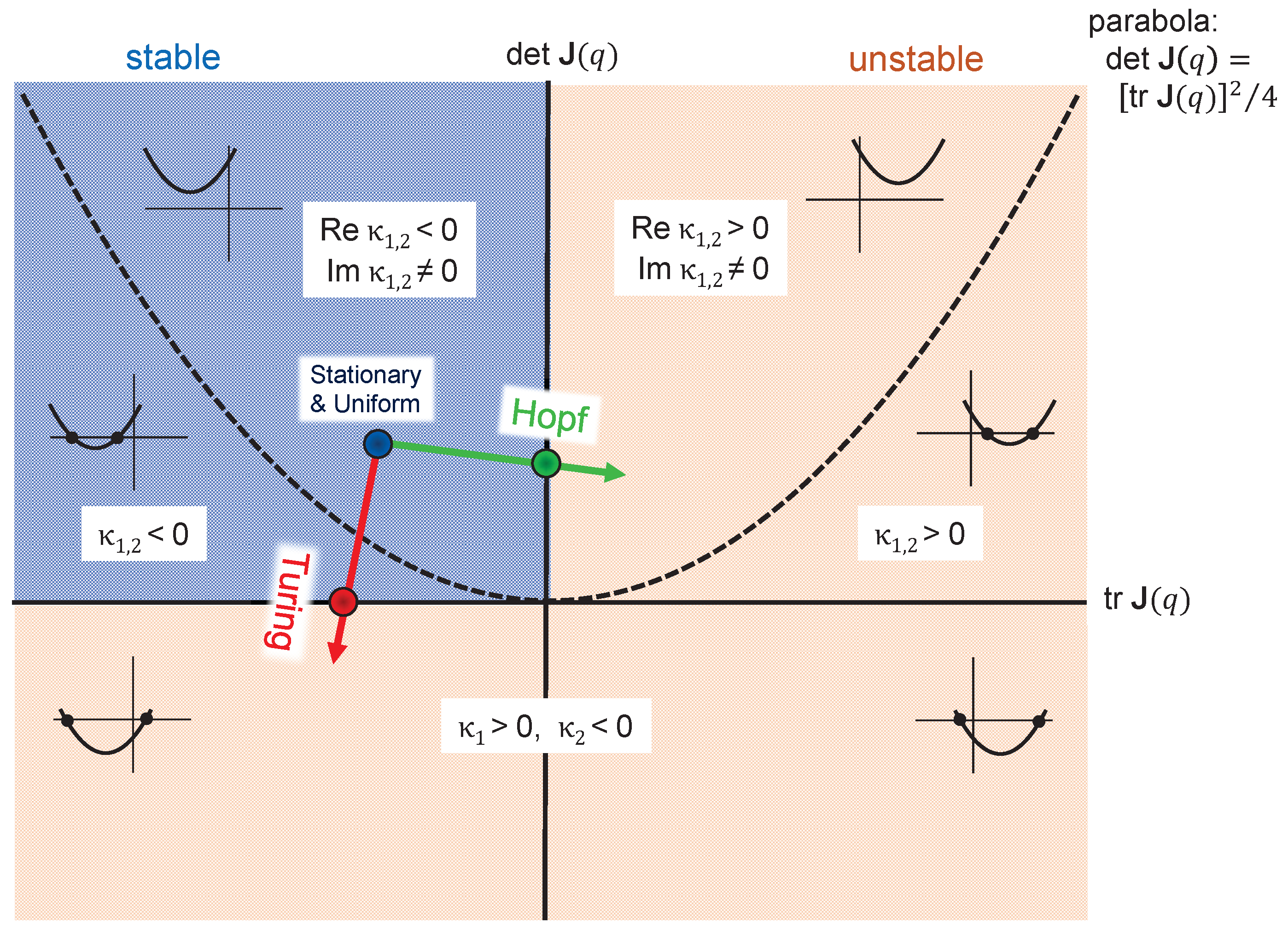
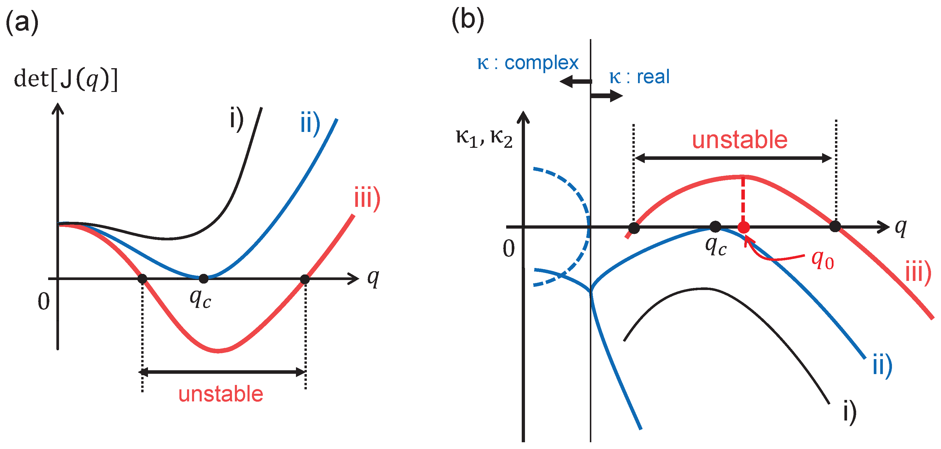
3.2. Occurrence Condition for Diffusion-Induced Instability

To proceed with analytic arguments, we expand the reaction terms $f({\rho }_s,{\rho }_m)$ and $g({\rho }_s,{\rho }_m)$ in Equation (1) around the stationary state ${\rho }_{s0}$ and ${\rho }_{m0}$ up to the first order. We then collect the zero-th and first terms only. Subsequently, it follows that the deviations ${\rho }_s^{*}={\rho }_s-{\rho }_{s0}$ and ${\rho }_m^{*}={\rho }_m-{\rho }_{m0}$ obey the linear equation

$${\partial }_t\left[\begin{array}{c}{\rho }_s^{*}\\ {\rho }_m^{*}\end{array}\right]={\partial }_x^2\left[\begin{array}{c}{D}_{sx}{\rho }_s^{*}\\ D_{mx}{\rho }_m^{*}\end{array}\right]+{\partial }_y^2\left[\begin{array}{c}{D}_{sy}{\rho }_s^{*}\\ D_{my}{\rho }_m^{*}\end{array}\right]+\left[\begin{array}{cc}{f}_s& f_m\\ g_s& g_m\end{array}\right]\left[\begin{array}{c}{\rho }_s^{*}\\ {\rho }_m^{*}\end{array}\right],$$

(2)

where the matrix elements in the last term of Equation (2) indicate the following partial derivative in the stationary state:

$$\begin{array}{c}{f}_s\equiv {\left.\frac{\partial f}{\partial {\rho }_s}\right|}_{{\rho }_s={\rho }_{s0},{\rho }_m={\rho }_{m0}},g_s\equiv {\left.\frac{\partial g}{\partial {\rho }_s}\right|}_{{\rho }_s={\rho }_{s0},{\rho }_m={\rho }_{m0}},\hfill \\ f_m\equiv {\left.\frac{\partial f}{\partial {\rho }_m}\right|}_{{\rho }_s={\rho }_{s0},{\rho }_m={\rho }_{m0}},g_m\equiv {\left.\frac{\partial g}{\partial {\rho }_m}\right|}_{{\rho }_s={\rho }_{s0},{\rho }_m={\rho }_{m0}}.\end{array}$$

(3)

Suppose that the spatiotemporal dependencies of both ${\rho }_j^{*}$$(j=s,m)$ can be expressed as

$$\begin{array}{c}\hfill \begin{array}{c}\hfill {\rho }_j^{*}(x,y,t)\propto e^{\kappa t}{e}^{-i\mathit{q}·\mathit{r}},\end{array}\end{array}$$

(4)

where $\mathit{q}=(q_x,q_y)$ and $\mathit{r}=(x,y)$. By substituting Equation (4) into Equation (2), the following secular equation is obtained:

$$\begin{array}{c}\hfill \begin{array}{c}\hfill det\left[\mathit{J}\left(\mathit{q}\right)-\kappa \mathit{I}\right]=0,\mathit{J}\left(\mathit{q}\right)=\left[\begin{array}{cc}-D_{sx}{q}_x^2-D_{sy}{q}_y^2+f_s& f_m\\ g_s& -D_{mx}{q}_x^2-D_{my}{q}_y^2+g_m\end{array}\right],\end{array}\end{array}$$

(5)

where $\mathit{I}$ denotes the identity matrix. The secular equation is alternatively expressed as follows:

$$\begin{array}{c}\hfill \begin{array}{c}\hfill {\kappa }^2-\mathrm{tr}\left[\mathit{J}\left(\mathit{q}\right)\right]\kappa +\det \left[\mathit{J}\left(\mathit{q}\right)\right]=0.\end{array}\end{array}$$

(6)

Equation (6) implies that the two eigenvalues, $\kappa ={\kappa }_1,{\kappa }_2$, are determined using the values of $\mathrm{tr}\left[\mathit{J}\right(\mathit{q}\left)\right]$ and $\det \left[\mathit{J}\right(\mathit{q}\left)\right]$. These two $\mathit{J}\left(\mathit{q}\right)$-dependent quantities are the functions of the the parameters involved in the reaction terms f and g and the diffusion constants $D_{ij}$ ($ij=sx,sy,mx,my$), as seen from Equation (5).

If the real parts of eigenvalues ${\kappa }_1$ and ${\kappa }_2$ are both negative, deviation, ${\rho }_j^{*}$$(j=s,m)$, from the stationary state decays with time (see Equation (4)). This decay means that even with density perturbations, the system returns to a stationary state. However, if at least one of the two eigenvalues has a positive real component, say $\mathrm{Re}\left({\kappa }_1\right)>0$, the deviation grows over time and may develop into a pattern with spatial periodicity. That is, the system exhibits diffusion-induced instability if the sign of the eigenvalue with the larger real part in Equation (6) changes from negative to positive by changing the values of the diffusion coefficients $D_{ij}$ ($ij=sx,sy,mx,my$) from all zero to at least one of them having a non-zero value.

Figure 3 shows the schematic diagram of the occurrence condition of diffusion-induced instability. The horizontal and vertical axes represent the values of $\mathrm{tr}\left[\mathit{J}\right(\mathit{q}\left)\right]$ and $\det \left[\mathit{J}\right(\mathit{q}\left)\right]$, respectively. Suppose that when $D_{ij}\equiv 0$, the system is positioned in the second quadrant labeled by the“stable” region, where $\mathrm{Re}\left({\kappa }_2\right)<\mathrm{Re}\left({\kappa }_1\right)<0$ such that the initial stationary state is stable. Once the diffusion effect becomes active, the system moves away from this position. If it moves downward in the phase diagram and crosses the horizontal axis, then the larger eigenvalue ${\kappa }_1$ is positive. Hence, the system undergoes Turing bifurcation. In equation form, diffusion-induced instability occurs if

$$\begin{array}{c}\hfill \begin{array}{c}\hfill \mathrm{tr}\left[\mathit{J}\right(\mathit{q}\left)\right]<0\mathrm{and}\det \left[\mathit{J}\right(\mathit{q}\left)\right]<0\mathrm{for}\mathrm{certain}\mathit{q}\ne \mathit{0},\end{array}\end{array}$$

(7)

while

$$\begin{array}{c}\hfill \begin{array}{c}\hfill \mathrm{tr}\left[\mathit{J}\right(\mathit{q}=0\left)\right]<0\mathrm{and}\det \left[\mathit{J}\right(\mathit{q}=0\left)\right]>0.\end{array}\end{array}$$

(8)

When the two conditions given in Equations (7) and (8) are satisfied, the eigenmodes of matrix $\mathit{J}\left(\mathit{q}\right)$ with a positive real part can grow over time with the help of diffusion and reaction of the components in the system. This eventually leads to the formation of a Turing pattern with a periodicity corresponding to the wave vector $\mathit{q}$, which makes $\det \left[\mathit{J}\right(\mathit{q}\left)\right]$ negative.

Figure 4 also schematically helps in understanding Turing bifurcation. Panel (a) presents the variation in $\det \left[J\right(q\left)\right]$ as a function of q; a one-dimensional system was considered for simplicity. In the initial stationary state, $\det \left[J\right(q\left)\right]$ is permanently positive regardless of whether q is (see curve (i) in Figure 4a). At the Turing bifurcation point (curve (ii)), the minimum value of $\det \left[J\right(q\left)\right]$ becomes zero at a certain q. Beyond bifurcation (curve (iii)), $\det \left[J\right(q\left)\right]$ takes a negative value in region q with a finite width. Within this region, the initial stationary state becomes unstable, so that the eigenmode with a positive real part can grow with time. The panel in Figure 4b shows the dispersion curves for cases (i), (ii), and (iii). On the right (left) side of the vertical thin line in the figure, eigenvalues ${\kappa }_1,{\kappa }_2$ are real (complex) numbers. It follows from Figure 4b that beyond the bifurcation, the larger eigenvalue ${\kappa }_1$ becomes positive within the limited “unstable” region where $\det \left[J\right(q\left)\right]<0$. Specifically, q that maximizes ${\kappa }_1(>0)$ is denoted by $q_0$. In principle, a spatial pattern with periodicity characterized by $q_0$ should grow the fastest because ${\kappa }_1$ is the largest. In a subsequent discussion (Section 4.3), we consider the growth of the periodic pattern characterized by $q_0$ in correlated dislocation systems.

4. Weakly Nonlinear Analysis

4.1. Defining the Reaction Terms for Dislocation Systems

We are now ready to address dislocation patterning from the perspective of Turing bifurcation. In order to analytically deal with the reaction–diffusion dynamics of individual dislocations under cyclic straining, we introduce the explicit forms of the reaction terms f and g given in [42] as

$$\begin{array}{ccc}f({\rho }_s,{\rho }_m)\hfill & =& \xi \left({\rho }_s\right)-\beta {\rho }_s+\gamma {\rho }_s^2{\rho }_m-b{\rho }_s^2-2c{\rho }_s^3,\hfill \end{array}$$

(9)

$$\begin{array}{ccc}g({\rho }_s,{\rho }_m)\hfill & =& \beta {\rho }_s-\gamma {\rho }_s^2{\rho }_m+c{\rho }_s^3,\hfill \end{array}$$

(10)

where the terms to the powers of ${\rho }_s$ and ${\rho }_m$ as well as the function $\xi \left({\rho }_s\right)$ (which is a polynomial of ${\rho }_s$, see below) represent the reactions between dislocations that occur under cyclic loading. The physical meaning of each term is explained in turn in the subsequent paragraphs and Figure 5.

The function $\xi \left({\rho }_s\right)$ given in Equation (9) represents the generation of slow dislocations from dislocation sources such as the Frank–Read type [52]. In this study, it is expressed using a polynomial expansion with respect to ${\rho }_s$ to the first order as

$$\begin{array}{c}\hfill \begin{array}{c}\hfill \xi \left({\rho }_s\right)\simeq \xi \left({\rho }_{s0}\right)-\alpha ({\rho }_s-{\rho }_{s0}),\alpha =-{\left.\frac{d\xi \left({\rho }_s\right)}{d{\rho }_s}\right|}_{{\rho }_s={\rho }_{s0}},\end{array}\end{array}$$

(11)

where $\xi \left({\rho }_{s0}\right)\equiv 0$ satisfies the stationary condition at ${\rho }_s={\rho }_{s0}$.

The parameter $\beta$ in Equations (9) and (10) represents the probability that the two dislocations consisting of a dipole are dissociated by a strong external shear stress and transform into two mobile dislocations (Figure 5a) [47,48,49]. Here, the number of dipole dissociations that occur per unit area per unit time is thought to be proportional to the number of dipoles included in the unit area. Owing to the separation of dipoles by the external shear stress, the density of slow dislocations decreases locally as expressed by the negative term of $-\beta {\rho }_s$ in Equation (9); in contrast, the density of mobile dislocations increased locally is written by the positive term $\beta {\rho }_s$ in Equation (10). Essentially, $\beta$ becomes operative when the external stress exceeds the attractive interactions between the constituent dislocations. During the cyclic loading experiment, a change in the dislocation pattern is observed by gradually increasing the externally applied shear stress. Following this observation, the parameter $\beta$ is regarded as the control parameter for the Turing bifurcation such that the change in the dislocation pattern is correlated with variation in the magnitude of $\beta$.

The parameter $\gamma$ in Equations (9) and (10) represents the probability of reaction in which one mobile dislocation is trapped by one dipole due to the three-body interaction between dislocations (Figure 5b). As mentioned in Section 2, a dipole generates a strain field around it, which can trap a mobile dislocation that approaches sufficiently close to the dipole from a particular direction [32]. The probability that this reaction occurs per unit time per unit area is proportional to the probability that one mobile dislocation and one dipole exist simultaneously in the unit area, thus being expressed by $\gamma {\rho }_s^2{\rho }_m$.

The parameters b and c imply the annihilation of slow dislocations contained in dipoles and tripoles, respectively. The annihilations are thought to occur owing to the thermally induced clime and glide motion of edge dislocations (Figure 5c); namely, dislocations that constitute a dipole (or tripole) can annihilate when external stress or thermal disturbance bring the distance between them much closer than the stable distance.

If the expansion of reaction terms f and g is truncated to the first order with respect to ${\rho }_s^{*}$ and ${\rho }_m^{*}$, the following linear matrix equation is obtained as

$$\begin{array}{c}\hfill \begin{array}{c}\hfill {\partial }_t{\mathit{\rho }}^{*}=\mathit{J}\left(\mathit{q}\right){\mathit{\rho }}^{*},\end{array}\end{array}$$

(12)

where ${\mathit{\rho }}^{*}={({\rho }_s^{*},{\rho }_m^{*})}^T$ and $\mathit{J}\left(\mathit{q}\right)$ is a matrix defined by Equation (5), with eigenvalues $\kappa ={\kappa }_1,{\kappa }_2$, where $\mathrm{Re}\left({\kappa }_1\right)>\mathrm{Re}\left({\kappa }_2\right)$. Hereafter, we denote the normalized eigenvectors corresponding to the eigenvalues as ${\mathit{w}}_1$ and ${\mathit{w}}_2$, respectively. Equation (12) implies that once $\mathrm{Re}\left({\kappa }_1\right)$ becomes positive by tuning the control parameters (such as $\beta$), the eigenmode of ${\mathit{w}}_1$ grows permanently and eventually diverges to infinity. Therefore, if a linear approximation is used, then it is not possible to correctly describe the system after a long period.

4.2. Defining the Nonlinear Vector–Matrix Equation

In the following discussion, we examine the contribution of the nonlinear terms included in the reaction terms for the dislocation patterns. To this end, we expand the two reaction terms to the third order. In the case of f, for instance, we obtain

$$\begin{array}{c}\hfill \begin{array}{c}\hfill f({\rho }_s,{\rho }_m)\simeq f({\rho }_{s0},{\rho }_{m0})+\sum _{p=1}^3\frac{1}{p!}{\left.{\left({\rho }_s^{*}\frac{\partial }{\partial {\rho }_s}+{\rho }_m^{*}\frac{\partial }{\partial {\rho }_m}\right)}^{p}f({\rho }_s,{\rho }_m)\right|}_{{\rho }_j={\rho }_{j0}},\end{array}\end{array}$$

(13)

where ${|}_{{\rho }_j={\rho }_{j0}}$ denotes the partial derivative in the stationary state of ${\rho }_j={\rho }_{j0}$$(j=s,m)$. A similar third-order expansion applies to $g({\rho }_s,{\rho }_m)$. Then, we obtain the following nonlinear vector–matrix equation:

$$\begin{array}{c}\hfill \begin{array}{c}\hfill {\partial }_t{\mathit{\rho }}^{*}=\mathit{J}\left(\mathit{q}\right){\mathit{\rho }}^{*}+{\mathcal{N}}_{30}\left({\mathit{\rho }}^{*}\right)+{\mathcal{N}}_{21}\left({\mathit{\rho }}^{*}\right)+{\mathcal{N}}_{20}\left({\mathit{\rho }}^{*}\right)+{\mathcal{N}}_{11}\left({\mathit{\rho }}^{*}\right),\end{array}\end{array}$$

(14)

where

$$\begin{gathered} {\mathcal{N}}_{30}\left({\mathit{\rho }}^{*}\right)=c\left(\begin{array}{c}-2{\left({\rho }_s^{*}\right)}^3\\ {\left({\rho }_s^{*}\right)}^3\end{array}\right),{\mathcal{N}}_{21}\left({\mathit{\rho }}^{*}\right)=-\gamma \left(\begin{array}{c}-{\left({\rho }_s^{*}\right)}^2{\rho }_m^{*}\\ {\left({\rho }_s^{*}\right)}^2{\rho }_m^{*}\end{array}\right), \\ {\mathcal{N}}_{20}\left({\mathit{\rho }}^{*}\right)=-\gamma {\rho }_{m0}\left(\begin{array}{c}-{\left({\rho }_s^{*}\right)}^2\\ {\left({\rho }_s^{*}\right)}^2\end{array}\right)+b\left(\begin{array}{c}-{\left({\rho }_s^{*}\right)}^2\\ 0\end{array}\right)+3c{\rho }_{s0}\left(\begin{array}{c}-2{\left({\rho }_s^{*}\right)}^2\\ {\left({\rho }_s^{*}\right)}^2\end{array}\right), \\ {\mathcal{N}}_{11}\left({\mathit{\rho }}^{*}\right)=-2\gamma {\rho }_{s0}\left(\begin{array}{c}-{\rho }_s^{*}{\rho }_m^{*}\\ {\rho }_s^{*}{\rho }_m^{*}\end{array}\right). \end{gathered}$$

(15)

The paired subscripts $mn$ attached to ${\mathcal{N}}_{mn}$ given in Equation (16) indicate that its vector components are associated with the partial differentiation in Equation (13) of the mth order with respect to ${\rho }_s$ and the nth order with respect to ${\rho }_m$.

Since Equation (14) is nonlinear, the exact solution cannot be analytically determined. Hence, we proceed with the following two steps. First, the state vector ${\mathit{\rho }}^{*}$ is assumed to be a scalar multiplication of ${\mathit{w}}_1$. This is justified because after a sufficiently long time has passed, the ${\mathit{w}}_2$ mode with a negative ${\kappa }_2$ decays, and only the ${\mathit{w}}_1$ mode with a positive ${\kappa }_1$ survives. Second, we represent all four vectors ${\mathcal{N}}_{mn}\left({\mathit{\rho }}^{*}\right)$ using a linear combination of the eigenvectors ${\mathit{w}}_1$ and ${\mathit{w}}_2$ and investigate the contribution of the ${\mathit{w}}_1$ component with the time evolution of ${\mathit{\rho }}^{*}$. In this way, we focus only on the fastest growing ${\mathit{w}}_1$ mode and the contribution of the nonlinear terms to the ${\mathit{w}}_1$ mode to approximately address the nonlinear effects of dislocation pattern formation.

4.3. Nonlinearity Effect on the Growth in Amplitude

The effect of the nonlinear component vectors ${\mathcal{N}}_{mn}\left({\mathit{\rho }}^{*}\right)$, listed in Equation (16), increases as the system departs from the Turing bifurcation point drawn in Figure 3. To investigate the effect on pattern formation, we focus on the fastest growing mode with the wave vector ${\mathit{q}}_0$ that maximizes the eigenvalue ${\kappa }_1\left({\mathit{q}}_0\right)>0$, which is located within the unstable region depicted in Figure 4.

After a sufficiently long time period, the ${\mathit{w}}_2$ mode with a negative ${\kappa }_2$ decays and eventually disappears, while the ${\mathit{w}}_1$ mode with a positive ${\kappa }_1$ survives. Under these circumstances, ${\mathit{\rho }}^{*}$ can be approximated as as a scalar multiple of ${\mathit{w}}_1$ as:

$$\begin{array}{c}\hfill \begin{array}{c}\hfill {\mathit{\rho }}^{*}(x,y,t)=\sigma (x,y,t){\mathit{w}}_1,\sigma (x,y,t)=\sum _{j=1}^3{a}_j\left(t\right)cos\left[{\mathit{q}}_j·\mathit{r}(x,y)\right],\end{array}\end{array}$$

(16)

where $\mathit{r}(x,y)$ is the position vector. In Equation (16), the amplitude $\sigma$ of the state ${\mathit{\rho }}^{*}$ is set to be the linear combination of the three allowed sinusoidal waves, labeled by j ($j=1,2,3$). Figure 6 illustrates the relative configurations of three wave vectors ${\mathit{q}}_j$; they are assumed to have the same magnitude as ${\mathit{q}}_0$ of the fastest growing mode but have different directions satisfying the three-fold rotational symmetry such that

$$\begin{array}{c}\hfill \begin{array}{c}\hfill \sum _{j=1}^3{\mathit{q}}_j=0,|{\mathit{q}}_j|=|{\mathit{q}}_{\mathit{0}}|\equiv q_0\mathrm{for}\mathrm{any}j.\end{array}\end{array}$$

(17)

The amplitude $\sigma$ is thus explicitly written as

$$\begin{array}{ccc}\hfill \sigma (x,y,t)& =& a_1\left(t\right)cos\left(q_{0}x\right)\hfill \\ & +& a_2\left(t\right)cos\left(-\frac{1}{2}{q}_{0}x+\frac{\sqrt{3}}{2}{q}_{0}y\right)\\ & +& a_3\left(t\right)cos\left(-\frac{1}{2}{q}_{0}x-\frac{\sqrt{3}}{2}{q}_{0}y\right).\end{array}$$

(18)

Note that the spatial distribution of ${\mathit{\rho }}^{*}$ as defined by Equation (16) corresponds to a 1D uniaxial ladder pattern if $a_1\ne 0$ and $a_2=a_3=0$, whereas it corresponds to a 2D spotted pattern with hexagonal symmetry if $a_1=a_2=a_3\ne 0$.

Further mathematical preparation for the subsequent discussion is the evaluation of the constants $S_j$ and $T_j$$(j=1,2)$ (see Appendix A) that satisfy the following relationship:

$${\mathcal{N}}_{20}\left({\mathit{w}}_1\right)+{\mathcal{N}}_{11}\left({\mathit{w}}_1\right)=S_1{\mathit{w}}_1+S_2{\mathit{w}}_2,$$

(19)

$${\mathcal{N}}_{30}\left({\mathit{w}}_1\right)+{\mathcal{N}}_{21}\left({\mathit{w}}_1\right)=T_1{\mathit{w}}_1+T_2{\mathit{w}}_2.$$

(20)

The coefficients $S_1$ and $T_1$ represent the degrees of contribution from the second- and third-order partial derivatives in Equation (13) to the fastest growing ${\mathit{w}}_1$ mode. The same explanation applies to $S_2$ and $T_2$. Using Equations (16), (19), and (20) and the definitions of ${\mathcal{N}}_{mn}$ given by Equation (16), we obtain

$${\mathcal{N}}_{20}\left({\mathit{\rho }}^{*}\right)+{\mathcal{N}}_{11}\left({\mathit{\rho }}^{*}\right)={\sigma }^2\left(S_1{\mathit{w}}_1+S_2{\mathit{w}}_2\right),$$

(21)

$${\mathcal{N}}_{30}\left({\mathit{\rho }}^{*}\right)+{\mathcal{N}}_{21}\left({\mathit{\rho }}^{*}\right)={\sigma }^3\left(T_1{\mathit{w}}_1+T_2{\mathit{w}}_2\right).$$

(22)

As ${\mathit{w}}_2$ decays rapidly with time, it suffices to only consider the contribution from ${\mathit{w}}_1$; this approximation enables us to rewrite the right sides of Equations (21) and (22) as

$${\mathcal{N}}_{20}\left({\mathit{\rho }}^{*}\right)+{\mathcal{N}}_{11}\left({\mathit{\rho }}^{*}\right)\sim {\sigma }^2{S}_1{\mathit{w}}_1,$$

(23)

$${\mathcal{N}}_{30}\left({\mathit{\rho }}^{*}\right)+{\mathcal{N}}_{21}\left({\mathit{\rho }}^{*}\right)\sim {\sigma }^3{T}_1{\mathit{w}}_1.$$

(24)

By substituting these function terms into Equation (14), we obtain

$$\begin{array}{c}\hfill \begin{array}{c}\hfill {\partial }_t\left({\sigma }_1{\mathit{w}}_1\right)\sim {\kappa }_1\sigma {\mathit{w}}_1+{\sigma }^2{S}_1{\mathit{w}}_1+{\sigma }^3{T}_1{\mathit{w}}_1.\end{array}\end{array}$$

(25)

By equating the coefficients on both sides of Equation (25), we obtain

$$\begin{array}{c}\hfill \begin{array}{c}\hfill {\partial }_t\sigma \sim {\kappa }_1\sigma +S_1{\sigma }^2+T_1{\sigma }^3.\end{array}\end{array}$$

(26)

Equation (26) determines the time evolution of the amplitude of the fastest growing mode ${\mathit{w}}_1$. If we set $S_1=T_1=0$, Equation (26) becomes a linear problem which implies that $\sigma$ grows permanently and diverges to infinity. The presence of $S_1$ and $T_1$ may suppress this divergence and, consequently, the amplitude converges to a finite value after sufficient time has passed. It also follows that for this suppression effect to occur, either S or T must be negative.

4.4. Time Evolution of the Amplitude

To determine the condition for the time-evolving amplitude $\sigma$ to converge to a constant value, we substitute the expression for $\sigma$ given by Equation (16) with Equation (26). We then apply the trigonometric formulas (see Appendix B) and the symmetry relation with respect to ${\mathit{q}}_j$ (see Equation (17)) to the cosine functions involved in the right-hand side of Equation (26). After that, we multiply both sides of Equation (26) by $cos({\mathit{q}}_n·\mathit{r})$ with an integer n ($1\le n\le 3$) and integrate on both sides with respect to $\mathit{r}$, which allows only the terms with satisfying $n=j$ to survive. Repeating this calculation while varying the n value from 1 to 3, we obtain the following set of three time-evolution equations [43,44]:

$$\frac{d{a}_1}{dt}={\kappa }_1{a}_1+S_1{a}_2{a}_3+\frac{3}{4}{T}_1\left[a_1^3+2a_1(a_2^2+a_3^2)\right],$$

(27)

$$\frac{d{a}_2}{dt}={\kappa }_1{a}_2+S_1{a}_3{a}_1+\frac{3}{4}{T}_1\left[a_2^3+2a_2(a_3^2+a_1^2)\right],$$

(28)

$$\frac{d{a}_3}{dt}={\kappa }_1{a}_3+S_1{a}_1{a}_2+\frac{3}{4}{T}_1\left[a_3^2+2a_3(a_1^2+a_2^2)\right].$$

(29)

The stability of the vector $\mathit{a}={(a_1,a_2,a_3)}^T$ can be examined by considering the linear vector–matrix equation of

$$\begin{array}{c}\hfill \begin{array}{c}\hfill \frac{d}{dt}\mathit{a}=\mathit{A}\mathit{a},\mathit{A}=\left(\begin{array}{ccc}{\left.\frac{\partial h_1}{\partial a_1}\right|}_{\mathit{a}={\mathit{a}}^{*}}& {\left.\frac{\partial h_1}{\partial a_2}\right|}_{\mathit{a}={\mathit{a}}^{*}}& {\left.\frac{\partial h_1}{\partial a_3}\right|}_{\mathit{a}={\mathit{a}}^{*}}\\ {\left.\frac{\partial h_2}{\partial a_1}\right|}_{\mathit{a}={\mathit{a}}^{*}}& {\left.\frac{\partial h_2}{\partial a_2}\right|}_{\mathit{a}={\mathit{a}}^{*}}& {\left.\frac{\partial h_2}{\partial a_3}\right|}_{\mathit{a}={\mathit{a}}^{*}}\\ {\left.\frac{\partial h_3}{\partial a_1}\right|}_{\mathit{a}={\mathit{a}}^{*}}& {\left.\frac{\partial h_3}{\partial a_2}\right|}_{\mathit{a}={\mathit{a}}^{*}}& {\left.\frac{\partial h_3}{\partial a_3}\right|}_{\mathit{a}={\mathit{a}}^{*}}\end{array}\right),h_j\equiv \frac{d{a}_j}{dt},\end{array}\end{array}$$

(30)

where ${\mathit{a}}^{*}$ denotes the stationary state with respect to $\mathit{a}$. If all three eigenvalues of the matrix $\mathit{A}$ are negative, the states located near ${\mathit{a}}^{*}$ will remain the same over time, which indicates growth saturation of the ${\mathit{w}}_1$ mode owing to nonlinear effects. Section 5 demonstrates the two cases in which the magnitude of $\mathit{a}$ does not diverge, but converges to a constant. Each of the two cases occur with the the emergence of 1D ladder-shaped and 2D spotted patterns.

5. Spot–Ladder Selection Rule

5.1. Condition for a “Ladder” Pattern to Appear

The appearance of a ladder pattern implies that the amplitudes of the three cosine terms converge to

$$\begin{array}{c}\hfill \begin{array}{c}\hfill a_1\ne 0\mathrm{and}{a}_2=a_3=0.\end{array}\end{array}$$

(31)

Hence, it follows from Equation (27) that

$$\begin{array}{c}\hfill \begin{array}{c}\hfill \frac{d{a}_1}{dt}={\kappa }_1{a}_1+\frac{3}{4}{T}_1{a}_1^3=0,\end{array}\end{array}$$

(32)

which implies

$$\begin{array}{c}\hfill \begin{array}{c}\hfill a_1\left({\kappa }_1+\frac{3}{4}{T}_1{a}_1^2\right)=0.\end{array}\end{array}$$

(33)

As $a_1\ne 0$, the convergence value of the amplitude $a_1$ is determined by

$$\begin{array}{c}\hfill \begin{array}{c}\hfill a_1=\pm \sqrt{\frac{4{\kappa }_1}{-3T_1}}.\end{array}\end{array}$$

(34)

This indicates that $T_1$ must be negative for $a_1$ to converge to a constant value. In the following sections, we rewrite $T_1^{\prime }\equiv -T_1>0$ for simplicity. Then, if the system prefers to enter a ladder pattern, $\mathit{a}$ converges to

$$\begin{array}{c}\hfill \begin{array}{c}\hfill {\mathit{a}}^{*}=\left(\begin{array}{c}\pm \sqrt{\frac{4{\kappa }_1}{3T_1^{\prime }}}\\ 0\\ 0\end{array}\right).\end{array}\end{array}$$

(35)

Substituting the results of Equation (35) into Equation (30), the matrix $\mathit{A}$ becomes

$$\begin{array}{c}\hfill \begin{array}{c}\hfill \mathit{A}=\left(\begin{array}{ccc}-2{\kappa }_1& 0& 0\\ 0& -{\kappa }_1& \pm 2S_1\sqrt{\frac{{\kappa }_1}{3T_1^{\prime }}}\\ 0& \pm 2S_1\sqrt{\frac{{\kappa }_1}{3T_1^{\prime }}}& -{\kappa }_1\end{array}\right),\end{array}\end{array}$$

(36)

whose eigenvalues are

$$\begin{array}{c}\hfill \begin{array}{c}\hfill -2{\kappa }_2,-{\kappa }_1\pm 2S_1\sqrt{\frac{{\kappa }_1}{3T_1^{\prime }}}.\end{array}\end{array}$$

(37)

Therefore, the condition for all three eigenvalues of $\mathit{A}$ to be negative is given by

$$\begin{array}{c}\hfill \begin{array}{c}\hfill |S_1|<\frac{\sqrt{3T_1^{\prime }{\kappa }_1}}{2},\end{array}\end{array}$$

(38)

or equivalently,

$$\begin{array}{c}\hfill \begin{array}{c}\hfill {\kappa }_1>\frac{4S_1^2}{3T_1^{\prime }}.\end{array}\end{array}$$

(39)

The inequality (39) serves as the condition for the 1D ladder pattern.

5.2. Condition for a “Spotted” Pattern to Appear

In the case of the emergence of the spotted pattern, the amplitudes of the three cosine terms converge to the same magnitude, represented by a, such that

$$\begin{array}{c}\hfill \begin{array}{c}\hfill a_1=a_2=a_3=a(\ne 0).\end{array}\end{array}$$

(40)

It then follows from Equation (27) that

$$\begin{array}{c}\hfill \begin{array}{c}\hfill \frac{da}{dt}={\kappa }_{1}a+S_1{a}^2+\frac{15}{4}{T}_1{a}^3=0,\end{array}\end{array}$$

(41)

which implies

$$\begin{array}{c}\hfill \begin{array}{c}\hfill a\left({\kappa }_1+S_{1}a+\frac{15}{4}{T}_1{a}^2\right)=0.\end{array}\end{array}$$

(42)

As $a\ne 0$, we have

$$\begin{array}{c}\hfill \begin{array}{c}\hfill a=\frac{2}{15T_1}\left(S_1\pm \sqrt{S_1^2-15T_1{\kappa }_1}\right)\mathrm{and}\mathrm{thus}{\mathit{a}}^{*}=\left(\begin{array}{c}a\\ a\\ a\end{array}\right).\end{array}\end{array}$$

(43)

In this case, the matrix $\mathit{A}$ becomes diagonal and its elements, denoted by $A_{ij}$ ($i,j=1,2,3$), are given by

$$\begin{array}{c}\hfill \begin{array}{c}\hfill A_{ij}=\left\{\begin{array}{cc}{\displaystyle {\kappa }_1+\frac{21}{4}{T}_1{a}^2,}& \mathrm{if}i=j,\\ & \\ S_{1}a+3T_1{a}^2,& \mathrm{otherwise}.\end{array}\right.\end{array}\end{array}$$

(44)

The $3\times 3$ diagonal matrix $\mathit{A}$ defined by Equation (44) is composed of all equal on-diagonal terms $A_{ii}$ and all equal off-diagonal terms $A_{ij}$$(j\ne i)$. Therefore, it has one doubly multiple root and another remaining root. The two roots, denoted by $z^{**}$ and $z^{*}$, are expressed as

$$\begin{array}{c}\hfill \begin{array}{c}\hfill z^{**}=A_{11}-A_{12}\left(\mathrm{doubly}\mathrm{multiple}\right),z^{*}=A_{11}+2A_{12}.\end{array}\end{array}$$

(45)

Their explicit forms are given by

$$\begin{array}{c}\hfill \begin{array}{c}\hfill z^{**}={\kappa }_1-S_{1}a+\frac{9}{4}{T}_1{a}^2,z^{*}={\kappa }_1+2S_{1}a+\frac{45}{4}{T}_1{a}^2,\end{array}\end{array}$$

(46)

where a denotes the value given in Equation (43).

The remaining task is to determine the appropriate conditions for both $z^{**}$ and $z^{*}$ to be negative. This task can be accomplished by eliminating a from Equation (46). Using the expression for a in Equation (43), we regard $z^{**}$ and $z^{*}$ as functions of $S_1$ with the positive constants ${\kappa }_1$ and $T_1^{\prime }\equiv -T_1$. After mathematical manipulation, we obtain

$$z^{**}<0\mathrm{if}\left|S_1\right|>\frac{\sqrt{3T_1^{\prime }{\kappa }_1}}{4},$$

(47)

$$z^{*}<0\mathrm{at}\mathrm{arbitrary}{S}_1.$$

(48)

In summary, all the eigenvalues of matrix $\mathit{A}$ are negative if

$$\begin{array}{c}\hfill \begin{array}{c}\hfill |S_1|>\frac{\sqrt{3T_1^{\prime }{\kappa }_1}}{4},\end{array}\end{array}$$

(49)

or equivalently

$$\begin{array}{c}\hfill \begin{array}{c}\hfill {\kappa }_1<\frac{16S_1^2}{3T_1^{\prime }}.\end{array}\end{array}$$

(50)

Inequality (50) serves as the condition for the 2D spotted pattern.

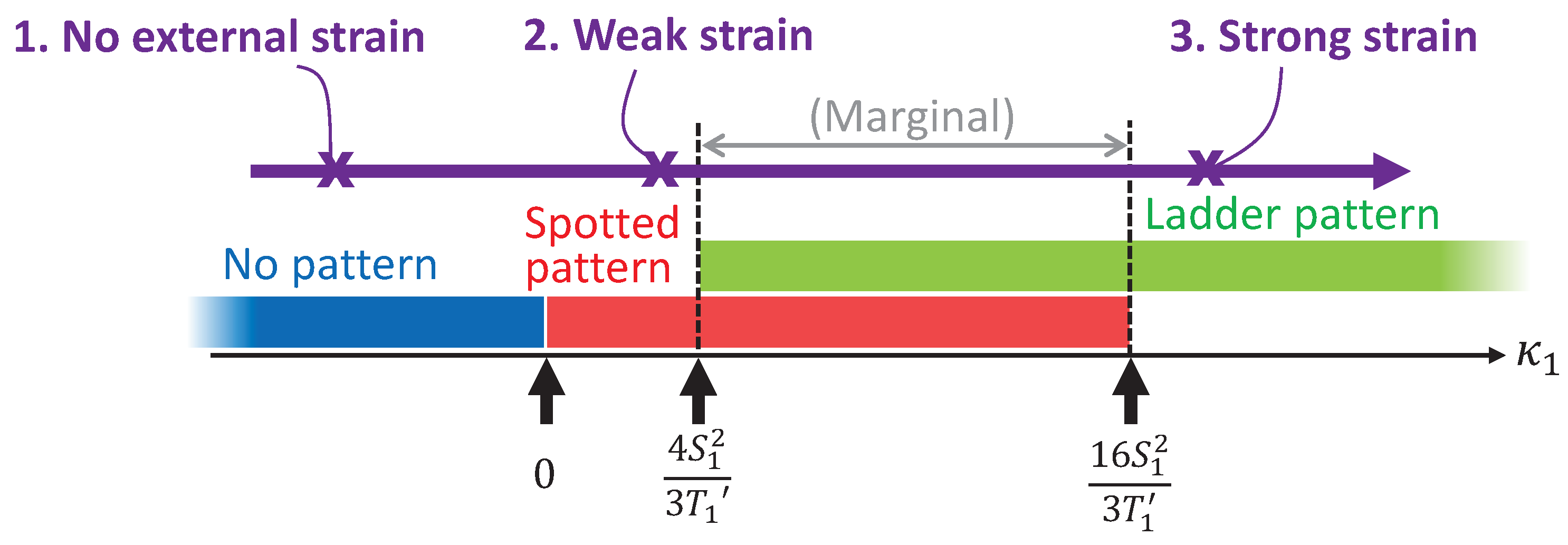
6. Selection Rule for “Spot vs. Ladder” Patterns

The types of dislocation patterns formed autonomously in fatigued metals in the small and medium strain amplitudes can be classified according to the magnitude relationship between the eigenvalue ${\kappa }_1$ and the nonlinear parameters $S_1$ and $T_1^{\prime }$:

$$\left(\mathrm{i}\right){\kappa }_1<0\Rightarrow \mathrm{no}\mathrm{pattern}\mathrm{grows}$$

(51)

$$\left(\mathrm{ii}\right)0<{\kappa }_1<\frac{4S_1^2}{3T_1^{\prime }}\Rightarrow \mathrm{spotted}\mathrm{pattern}\mathrm{emerges}$$

(52)

$$\left(\mathrm{iii}\right)\frac{4S_1^2}{3T_1^{\prime }}<{\kappa }_1<\frac{16S_1^2}{3T_1^{\prime }}\Rightarrow \mathrm{marginal}\left(\mathrm{both}\mathrm{patterns}\mathrm{may}\mathrm{appear}\right)$$

(53)

$$\left(\mathrm{iv}\right)\frac{16S_1^2}{3T_1^{\prime }}<{\kappa }_1\Rightarrow \mathrm{ladder}\mathrm{pattern}\mathrm{emerges}$$

(54)

Figure 7 shows a bifurcation diagram that schematically illustrates the type of spatially periodic pattern preferred for a given parameter. The horizontal axis indicates the eigenvalue ${\kappa }_1$, whose magnitude characterizes the strength of the externally applied shear stress, as mentioned in Section 4.1. This diagram shows the presence of four distinct phases. Each of these phases corresponds to a dislocation pattern with a different geometric symmetry.

The bifurcation diagram shown in Figure 7 is of particular interest because it is in qualitative agreement with the experimental observations. In the cyclic loading experiments, it was observed that the shape of the dislocation pattern changed gradually. The pattern shifted from a spotted pattern to a ladder-like pattern as the applied strain stress increased. Furthermore, a marginal pattern, in which both patterns were mixed in the same specimen, was experimentally observed. In this marginal pattern, an increased shear stress leads to a decrease in the area occupied by the spotted pattern across the entire cross-section of the specimen, whereas it leads to an increase in the area occupied by the ladder pattern. This gradual change in the dominant pattern with increasing stress is shown in the bifurcation diagram presented in Figure 7.

7. Summary

In this study, a bifurcation diagram was derived that explains the crossover from the 2D spotted pattern to the 1D ladder-shaped pattern observed in fatigued metals under cyclic loading conditions. Thresholds separating the different patterns were formulated as functions of nonlinearity parameters defined by $S_1$ and $T_1^{\prime }$, which characterize the degree of nonlinear effects from the creation and annihilation of dislocations inside the system. The bifurcation diagram that was developed implies a gradual change in the geometric characteristics of the patterns with increasing applied shear stress and is consistent with experimental observations.

It should be emphasized that the model presented provides a conceptual framework to study the formation of dislocation patterns formed as a result of the competition between nonlinear interactions of dislocations and stress-enhanced dissociation of multipoles. Nevertheless, qualitative agreement with experimental results alone is not sufficient for the model to be accepted as reliable; quantitative agreement between theory and experiment also needs to be scrutinized using realistic parameter values [53]. In addition, when considering a realistic metallic specimen of a finite size, it is necessary to consider the attractive force exerted by the outer surface of the specimen on the dislocations inside [54,55]. To accomplish these tasks, numerical simulations based on coupled differential equations will be discussed in future work.

References

1. Cross, M.C.; Hohenberg, P.C. Pattern formation outside of equilibrium. Rev. Mod. Phys. 1993, 65, 851–1112. [Google Scholar] [CrossRef]
2. Turing, A. The chemical basis of morphogenesis. Philos. Trans. R. Soc. Lond. Ser. B 1952, 237, 37–72. [Google Scholar] [CrossRef]
3. Greif, H.; Kubiak, A.; Stacewicz, P. Turing’s biological philosophy: Morphogenesis, mechanisms and organicism. Philosophies 2023, 8, 8. [Google Scholar] [CrossRef]
4. Gierer, A.; Meinhardt, H. A theory of biological pattern formation. Kybernetik 1972, 12, 30–39. [Google Scholar] [CrossRef] [PubMed]
5. Landge, A.N.; Jordan, B.M.; Diego, X.; Muller, P. Pattern formation mechanisms of self-organizing reaction-diffusion systems. Dev. Biol. 2020, 460, 2–11. [Google Scholar] [CrossRef]
6. Kondo, S.; Miura, T. Reaction-diffusion model as a framework for understanding biological pattern formation. Science 2010, 329, 1616–1620. [Google Scholar] [CrossRef]
7. Maini, P.K.; Painter, K.J.; Chau, H.N.P. Spatial pattern formation in chemical and biological systems. J. Chem.-Soc.-Faraday Trans. 1997, 93, 3601–3610. [Google Scholar] [CrossRef]
8. Murray, J.D. Mathematical Biology; Springer: Berlin/Heidelberg, Germany, 2002. [Google Scholar]
9. Nakamasu, A.M. Correspondences Between Parameters in a Reaction-Diffusion Model and Connexin Functions During Zebrafish Stripe Formation. Front. Phys. 2022, 9, 805659. [Google Scholar] [CrossRef]
10. Morita, W.; Morimoto, N.; Otsu, K.; Miura, T. Stripe and spot selection in cusp patterning of mammalian molar formation. Sci. Rep. 2022, 12, 9149. [Google Scholar] [CrossRef]
11. Toxvaerd, S. The emergence of the bilateral symmetry in animals: A review and a new hypothesis. Symmetry 2021, 13, 261. [Google Scholar] [CrossRef]
12. Castets, V.V.; Dulos, E.; Boissonade, J.; De Kepper, P. Experimental evidence of a sustained standing Turing-type nonequilibrium chemical pattern. Phys. Rev. Lett. 1990, 64, 2953–2956. [Google Scholar] [CrossRef] [PubMed]
13. Ouyang, Q.; Swinney, H.L. Transition from a uniform state to hexagonal and striped Turing patterns. Nature 1991, 352, 610–612. [Google Scholar] [CrossRef]
14. Horváth, J.; Szalai, I.; De Kepper, P. An experimental design method leading to chemical Turing patterns. Science 2009, 324, 772–775. [Google Scholar] [CrossRef] [PubMed]
15. Ali, I.; Saleem, M.T. Spatiotemporal dynamics of reaction-diffusion system and its application to Turing pattern formation in a Gray-Scott model. Mathematics 2023, 11, 1459. [Google Scholar] [CrossRef]
16. Fang, A.; Adamo, C.; Jia, S.; Cava, R.J.; Wu, S.C.; Felser, C.; Kapitulnik, A. Bursting at the seams: Rippled monolayer bismuth on NbSe2. Sci. Adv. 2018, 4, eaaq0330. [Google Scholar] [CrossRef] [PubMed]
17. Fuseya, Y.; Katsuno, H.; Behnia, K.; Kapitulnik, A. Nanoscale Turing patterns in a bismuth monolayer. Nat. Phys. 2021, 17, 1031. [Google Scholar] [CrossRef]
18. Bandyopadhyay, B.; Khatun, T.; Banerjee, T. Quantum Turing bifurcation: Transition from quantum amplitude death to quantum oscillation death. Phys. Rev. E 2021, 104, 024214. [Google Scholar] [CrossRef]
19. Kato, Y.; Nakao, H. Turing instability in quantum activator-inhibitor systems. Sci. Rep. 2022, 12, 15573. [Google Scholar] [CrossRef]
20. Suresh, S. Fatigue of Metals; Cambridge University Press: Cambridge, UK, 1998. [Google Scholar]
21. Li, P.; Li, S.X.; Wang, Z.G.; Zhang, Z.F. Fundamental factors on formation mechanism of dislocation arrangements in cyclically deformed fcc single crystals. Prog. Mater. Sci. 2011, 56, 328–377. [Google Scholar] [CrossRef]
22. Deng, X.; Xiao, Y.; Ma, Y.; Huang, B.; Hu, W. The microstructural evolution of nickel single crystal under cyclic deformation and hyper-gravity conditions: A molecular dynamics study. Metals 2022, 12, 1128. [Google Scholar] [CrossRef]
23. Cleja-Ţigoiu, S. Differential Geometry Approach to Continuous Model of Micro-Structural Defects in Finite Elasto-Plasticity. Symmetry 2021, 13, 2340. [Google Scholar] [CrossRef]
24. Lazar, M. Displacements and Stress Functions of Straight Dislocations and Line Forces in Anisotropic Elasticity: A New Derivation and Its Relation to the Integral Formalism. Symmetry 2021, 13, 1721. [Google Scholar] [CrossRef]
25. Polák, J. Role of persistent slip bands and persistent slip markings in fatigue crack initiation in polycrystals. Crystals 2023, 13, 220. [Google Scholar] [CrossRef]
26. Ananthakrishna, G. Current theoretical approaches to collective behavior of dislocations. Phys. Rep. 2007, 440, 113–259. [Google Scholar] [CrossRef]
27. Sumigawa, T.; Uegaki, S.; Yukishita, T.; Arai, S.; Takahashi, Y.; Kitamura, T. FE-SEM in situ observation of damage evolution in tension-compression fatigue of micro-sized single-crystal copper. Mater. Sci. Eng. A 2019, 764, 138218. [Google Scholar] [CrossRef]
28. Winter, A.T. A model for the fatigue of copper at low plastic strain amplitudes. Philos. Mag. 1974, 30, 719–738. [Google Scholar] [CrossRef]
29. Mughrabi, H. The cyclic hardening and saturation behaviour of copper single crystals. Mater. Sci. Eng. 1978, 33, 207–223. [Google Scholar] [CrossRef]
30. Differt, K.; Essmann, U. Dynamical model of the wall structure in persistent slip bands of fatigued metals I. Dynamical model of edge dislocation walls. Mater. Sci. Eng. A 1993, 164, 295–299. [Google Scholar] [CrossRef]
31. Essmann, U.; Differt, K. Dynamic model of the wall structure in persistent slip bands of fatigued metals II. The wall spacing and the temperature dependence of the yield stress in saturation. Mater. Sci. Eng. A 1996, 208, 56–68. [Google Scholar] [CrossRef]
32. Kroupa, F. Dislocation Dipoles and Dislocation Loops. J. Phys. 1966, 27, 154–167. [Google Scholar] [CrossRef]
33. Neumann, P.D. The interactions between dislocations and dislocation dipoles. Acta Metall. 1971, 19, 1233–1241. [Google Scholar] [CrossRef]
34. Siddique, A.B.; Lim, H.; Khraishi, T.A. The Effect of Multipoles on the Elasto-Plastic Properties of a Crystal: Theory and Three-Dimensional Dislocation Dynamics Modeling. J. Eng. Mater. Technol. 2022, 144, 011016. [Google Scholar] [CrossRef]
35. Feltner, C.E. A debris mechanism of cyclic strain hardening for F.C.C. metals. Philos. Mag. 1965, 12, 1229–1248. [Google Scholar] [CrossRef]
36. Erel, C.; Po, G.; Crosby, T.; Ghoniem, N. Generation and interaction mechanisms of prismatic dislocation loops in FCC metals. Comput. Mater. Sci. 2017, 140, 32–46. [Google Scholar] [CrossRef]
37. Torrisi, M.; Tracinà, R. Symmetries and Solutions for Some Classes of Advective Reaction-Diffusion Systems. Symmetry 2022, 14, 2009. [Google Scholar] [CrossRef]
38. Shao, S.; Du, B. Global Asymptotic Stability of Competitive Neural Networks with Reaction-Diffusion Terms and Mixed Delays. Symmetry 2022, 14, 2224. [Google Scholar] [CrossRef]
39. Alderremy, A.A.; Shah, R.; Iqbal, N.; Aly, S.; Nonlaopon, K. Fractional Series Solution Construction for Nonlinear Fractional Reaction-Diffusion Brusselator Model Utilizing Laplace Residual Power Series. Symmetry 2022, 14, 1944. [Google Scholar] [CrossRef]
40. Trochidis, A.; Douka, E.; Polyzos, B. Formation and evolution of persistent slip bands in metals. J. Mech. Phys. Solids 2000, 48, 1761–1775. [Google Scholar] [CrossRef]
41. Aoyagi, Y.; Kobayashi, R.; Kaji, Y.; Shizawa, K. Modeling and simulation on ultrafine-graining based on multiscale crystal plasticity considering dislocation patterning. Int. J. Plast. 2013, 47, 13–28. [Google Scholar] [CrossRef]
42. Walgraef, D.; Aifantis, E.C. Dislocation Patterning in Fatigued Metals as a Result of Dynamical Instabilities. J. Appl. Phys. 1985, 58, 688–691. [Google Scholar] [CrossRef]
43. Ermentrout, B. Stripes or spots? Nonlinear effects in bifurcation of reaction-diffusion equations on the square. Proc. R. Soc. Lond. Ser. A 1991, 434, 413–417. [Google Scholar] [CrossRef]
44. Lyons, M.J.; Harrison, L.G. Stripe selection: An intrinsic property of some pattern-forming models with nonlinear dynamics. Dev. Dyn. 1992, 195, 201–215. [Google Scholar] [CrossRef] [PubMed]
45. Barrio, R.A.; Varea, C.; Aragon, J.L.; Maini, P.K. A two-dimensional numerical study of spatial pattern formation in interacting Turing systems. Bull. Math. Biol. 1999, 61, 483–505. [Google Scholar] [CrossRef]
46. Shoji, H.; Iwasa, Y.; Kondo, S. Stripes, spots, or reversed spots in two-dimensional Turing systems. J. Theor. Biol. 2003, 224, 339–350. [Google Scholar] [CrossRef]
47. Walgraef, D.; Aifantis, E.C. On the Formation and Stability of Dislocation Patterns.1. One-Dimensional Considerations. Int. J. Eng. Sci. 1985, 23, 1351–1358. [Google Scholar] [CrossRef]
48. Walgraef, D.; Aifantis, E.C. On the Formation and Stability of Dislocation Patterns.2. Two-Dimensional Considerations. Int. J. Eng. Sci. 1985, 23, 1359–1364. [Google Scholar] [CrossRef]
49. Walgraef, D.; Aifantis, E.C. On the Formation and Stability of Dislocation Patterns.3. 3-Dimensional Considerations. Int. J. Eng. Sci. 1985, 23, 1365–1372. [Google Scholar] [CrossRef]
50. Schiller, C.; Walgraef, D. Numerical-Simulation of Persistent Slip Band Formation. Acta Metall. 1988, 36, 563–574. [Google Scholar] [CrossRef]
51. Pontes, J.; Walgraef, D.; Aifantis, E.C. On dislocation patterning: Multiple slip effects in the rate equation approach. Int. J. Plast. 2006, 22, 1486–1505. [Google Scholar] [CrossRef]
52. Anderson, P.M.; Hirth, J.P.; Lothe, J. Theory of Dislocations; Cambridge University Press: Cambridge, UK, 2017. [Google Scholar]
53. Umeno, Y.; Kawai, E.; Kubo, A.; Shima, H.; Sumigawa, T. Inductive determination of rate-reaction equation parameters for dislocation structure formation using artificial neural network. Materials 2023, 16, 2108. [Google Scholar] [CrossRef]
54. Shima, H.; Umeno, Y.; Sumigawa, T. Analytic formulation of elastic field around edge dislocation adjacent to slanted free surface. R. Soc. Open Sci. 2022, 9, 220151. [Google Scholar] [CrossRef] [PubMed]
55. Shima, H.; Sumigawa, T.; Umeno, Y. Nonsingular stress distribution of edge dislocations near zero-traction boundary. Materials 2022, 15, 4929. [Google Scholar] [CrossRef] [PubMed]
Figure 1. Drawings of the three types of dislocation patterns observed at the cross-section of fatigued metals: (a) spotted pattern, (b) vein pattern, (c) ladder pattern that appears between two parallel dashed lines. Dislocations are densely distributed in the grey area, but are sparse in the white area. In material science, the ladder pattern shown in panel (c) is commonly called the “persistent slip band (PSB) ladder” structure.
Symmetry 15 01028 g001
Figure 2. (a) Flip-flop motion inside an edge-dislocation dipole between two stable configurations labeled by P and Q. (b) Four stable configurations of an edge-dislocation tripole. The panels from I to IV display the four different relative positions of the third edge dislocation to the dipole connected by the dashed line.
Symmetry 15 01028 g002
Figure 3. Diagram for the occurrence conditions of diffusion-induced instability (i.e., Turing bifurcation). The six small downward parabolas embedded in the diagram illustrate the sign of the real part of the eigenvalues κ 1 and κ 2 in each region as well as the presence/absence of the imaginary part. The initial stationary state is stable with time if it is located in the second quadrant, otherwise it is unstable. A Turing pattern may start to grow if the system transitions from the second to third quadrant by changing the parameter involved in the matrix J ( q ) defined by Equation (5). Transit from the second to first quadrant triggers another class of bifurcation (temporally oscillating), called the Hopf bifurcation, which is beyond the scope of this work.
Symmetry 15 01028 g003
Figure 4. (a) Variation in det [ J ( q ) ] for three cases: (i) at the initial stationary state; (ii) on the Turing bifurcation point; (iii) beyond the bifurcation. The closed region at which det [ J ( q ) ] < 0 is an unstable region, where the stationary state becomes unstable so that a certain periodic pattern may take place. (b) Dispersion curves that relate the eigenvalues κ of the matrix J ( q ) and the wavevector q. κ is complex (real) valued to the left (right) of the vertical thin line. The specific q that maximizes κ 1 ( > 0 ) within the unstable region of (iii) is labeled by q 0 , characterizing the fastest growing eigenmode.
Symmetry 15 01028 g004
Figure 5. Interaction between dislocations presumed to occur inside metals undergoing fatigue. (a) Cyclic-loading-induced liberation of slow dislocations (e.g., dipoles) into mobile ones. (b) Capturing of mobile dislocation by a dipole through the attractive force. (c) Annihilation of paired dislocations within a multipole.
Symmetry 15 01028 g005
Figure 6. Schematic definition of the wave vectors q j ( j = 1 , 2 , 3 ) given by Equation (16). The unit vectors e x and e y are also drawn.
Symmetry 15 01028 g006
Figure 7. Bifurcation diagram of the dislocation pattern. An increase in the eigenvalue κ 1 corresponds to an increase in shear stress in the cyclic loading experiment. See text for the definitions of S 1 and T 1 .
Symmetry 15 01028 g007
Disclaimer/Publisher’s Note: The statements, opinions and data contained in all publications are solely those of the individual author(s) and contributor(s) and not of MDPI and/or the editor(s). MDPI and/or the editor(s) disclaim responsibility for any injury to people or property resulting from any ideas, methods, instructions or products referred to in the content.