Spectral Characterization of Graphs with Respect to the Anti-Reciprocal Eigenvalue Property

Abstract

Let $G=(V,E)$ be a simple connected graph with vertex set V and edge set E, respectively. The term “anti-reciprocal eigenvalue property“ refers to a non-singular graph G for which, $-\frac{1}{\lambda }\in \sigma \left(G\right)$, whenever $\lambda \in \sigma \left(G\right)$, $\forall \lambda \in \sigma \left(G\right)$. Here, $\sigma \left(G\right)$ is the multiset of all eigenvalues of $A\left(G\right)$. Moreover, if multiplicities of eigenvalues and their negative reciprocals are equal, then that graph is said to have strong anti-reciprocal eigenvalue properties, and the graph is referred to as a strong anti-reciprocal graph (or $(-SR)$ graph). In this article, a new family of graphs $F_n^{(k,j)}$ is introduced and the energy of $F_5^{(k,\frac{k}{2})}$$k\ge 2$ is calculated. Furthermore, with the help of $F_5^{(k,\frac{k}{2})}$, some families of $(-SR)$ graphs are constructed.

1. Introduction

Spectral graph theory is concerned with the study of the eigenvalues associated with various matrices for a graph and how the eigenvalues relate to the structural characteristics of the graph. The spectrum of a graph is related to properties such as connectedness, diameter, independence number, chromatic number, and regularity. Many scholars have investigated the spectral characteristics of (adjacency matrices of) graphs; see [1,2,3,4,5,6,7,8,9,10,11]. Let G be the graph, such that $\left|V\right(G\left)\right|=n$ and

$$A\left(G\right)={\left[a_{ij}\right]}_{n\times n}=\left\{\begin{array}{cc}1,\hfill & \mathrm{if}i\mathrm{and}j\mathrm{are}\mathrm{adjacent};\hfill \\ 0,\hfill & \mathrm{otherwise},\hfill \end{array}\right.$$

be the adjacency matrix of graph G, which is square and symmetric; hence, its eigenvalues are all real. A singular graph G is a graph for which $\left|A\right(G\left)\right|=0$, otherwise, it is referred to as non-singular. The characteristic polynomial $P(G;\lambda )$ of graph G can be obtained from $A\left(G\right)$. The eigenvalues of $A\left(G\right)$, or simply the eigenvalues of graph G, are the roots of this polynomial. The spectrum (or the multiset of all eigenvalues) of graph G throughout the text is defined as

$$\sigma \left(G\right)=\left(\begin{array}{cccc}{\lambda }_1& {\lambda }_2& \dots & {\lambda }_n\\ m_1& m_2& \dots & m_n\end{array}\right),$$

where ${\lambda }_1\left(G\right)\ge {\lambda }_2\left(G\right)\ge \dots \ge {\lambda }_n\left(G\right)$, and $m_i$ is the multiplicity of each ${\lambda }_i$ for $i=1,2,\dots ,n$. It is well known that graph G is bipartite if and only if its nonzero eigenvalues are symmetric around 0. The sum of all absolute eigenvalues of graph G is called the energy of a graph, denoted by $E\left(G\right)$.

Definition 1 ([12]).

The anti-reciprocal eigenvalue property (or property $(-R)$) is said to hold by graph G if for each $\lambda \in \sigma \left(G\right)$ there exists $-\frac{1}{\lambda }\in \sigma \left(G\right)$. The multiplicities of the eigenvalues and their negative reciprocals may or may not be equal for graph G with property $(-R)$; however, if each eigenvalue and its negative reciprocal have the same multiplicities, graph G is said to satisfy a strong anti-reciprocal eigenvalue (or property $(-SR)$).

Definition 2 ([13]).

The reciprocal eigenvalue property (or property $\left(R\right)$) is said to hold by graph G if for each $\lambda \in \sigma \left(G\right)$ there exists $\frac{1}{\lambda }\in \sigma \left(G\right)$. The multiplicities of the eigenvalues and their reciprocals may or may not be equal for graph G with property $\left(R\right)$; however, if each eigenvalue and its reciprocal have the same multiplicities, then that graph G is said to satisfy the strong reciprocal eigenvalue (or property $\left(SR\right)$).

Note that if graph G is a bipartite graph, then properties $(-SR)$ and $\left(SR\right)$ are symmetric around 0. The adjacency matrix of a simple connected graph is symmetric. This fact is useful for converting the adjacency matrix into a block matrix. Furthermore, this block form of the adjacency matrix is useful for computing the characteristic polynomials of the graph.

Graph G satisfying property $\left(R\right)$ (respectively, property $\left(SR\right)$) is referred to as the reciprocal graph (respectively, strong reciprocal graph), and abbreviated as the $\left(R\right)$ graph (respectively, $\left(SR\right)$ graph). Graph G satisfying property $(-R)$ (respectively, property $(-SR)$) is referred to as an anti-reciprocal graph (respectively, strong anti-reciprocal graph), and abbreviated as $(-R)$ graph (respectively, $(-SR)$ graph).

It is well known that graph G is bipartite if and only if, for each eigenvalue $\lambda$, there exits $-\lambda$ in the spectrum of G. In 1978, the authors investigated property $\left(SR\right)$ for non-singular trees in [14] and [15], respectively, but with different names, i.e., “symmetric property” and “property C”, respectively. Later, Barik et al. [16] renamed this property as property $\left(SR\right)$ in 2006 and introduced property $\left(R\right)$. They proved that properties $\left(R\right)$ and $\left(SR\right)$ are equal in the case of nonsingular trees. Researchers investigated these properties for weighted trees in [17] and a subclass of connected bipartite graphs (with a unique perfect matching) in [18]. They showed that if we apply appropriate limitations on weight functions, these two properties are equal; however, in general, these properties are not the same, see [19]. Unicyclic graphs with property $\left(SR\right)$ were studied in [20]. It is worth noting that the study of reciprocal eigenvalue properties is strongly related to the concepts of ‘matching’ and ‘corona product’, which are both widely studied disciplines.

Definition 3 ([21]).

Consider two simple connected graphs, i.e., $G_1$ and $G_2$ of orders $n_1$ and $n_2$, respectively. The corona product $G_1\circ G_2$ of graphs $G_1$ and $G_2$ is a graph constructed with the help of one copy of graph $G_1$ and $n_1$-copies of $G_2$ and then connecting each vertex of the $ith$ copy of $G_2$ with the $ith$ vertex of $G_1$, where $1\le i\le n_1$.

In 2012, Lagrange [12] introduced the strong anti-reciprocal eigenvalue property for graphs and investigated this property for zero-divisor graphs of finite commutative rings with non-zero divisors. In [22], the authors investigated a family of graphs with a unique perfect matching M, where the diagonal entries of the inverse of the adjacency matrix of each graph were all zero. Moreover, it was proved that each non-corona graph in this class did not satisfy the property $(-SR)$, even for a single weight function $w\in W\left(G\right)$.

In 2017, Ahmad et al. investigated a class of weighted graphs($G_M$) with a unique perfect matching M [23]. They proved that the weighted graph $G_w$ of a graph $G\in G_M$ satisfies property $(-SR)$ for all $w\in W\left(G\right)$ if and only if G is a corona graph.

In [24], the authors raised the question of “whether non-corona graphs with the property $(-SR)$ exist?” and then answered this question by constructing seven types of unweighted non-corona graphs that satisfy property $(-SR)$. These constructions were later generalized by Barik et al. in [25] for unweighted graphs; in [26], the authors investigated property $(-SR)$ for the generalized families constructed in [25] with a specific weight function. In [27], the authors investigated some new families of non-corona graphs with property $(-SR)$.

The study of graph theory has led to significant advancements in various fields, ranging from computer science to social networks. However, there is a constant pursuit to uncover new families of graphs that possess unique properties and offer fresh insights into the underlying structures of complex networks. In this vein, a novel family of graphs, called flabellum graphs, was introduced. By investigating and analyzing the properties of flabellum graphs, such as their connectivity, energy, and degree sequences, the aim is to contribute to the ever-growing body of knowledge in graph theory. Furthermore, the construction of several families of $(-SR)$ graphs can be facilitated using the flabellum graph network. Additionally, by evaluating the energies associated with these graphs, we are exploring the intricate relationship between their structural attributes and their physical properties. The following concepts will be used in the next section.

Definition 4.

The Dutch windmill graph $D_n^{\left(k\right)}$, $k\ge 2$, $n\ge 3$, is the graph obtained by taking k copies of the cycle $C_n$ with a vertex in common.

Lemma 1 ([23]).

A polynomial $f\left(t\right)={\sum }_{j=0}^{2n}{a}_j{t}^j$ is said to satisfy property $(-SR)$ if and only if

$$\begin{array}{c}\hfill a_{2n-j}=\left\{\begin{array}{cc}{a}_j,\hfill & if j and n have the same parity,\hfill \\ \\ -a_j,\hfill & otherwise.\hfill \end{array}\right.j=0,1,2,\dots ,2n.\end{array}$$

The following lemmas will be used to prove our main results.

Lemma 2 ([28]).

Let A be an $n\times n$ matrix and $1\le k<n.$ Then for any constant c,

$$\begin{gathered} det(A+\left[\begin{array}{cc}c{I}_k& O\\ O& O\end{array}\right]) \\ =\left|A\right|+c{\sum }_{i=1}^{k}det\left(A\left[i\right]\right)+c^2\left(\genfrac{}{}{0pt}{}{k}{2}\right){\sum }_{i,j=1}^{k}det\left(A[i,j]\right)+\cdots +c^k\left(\genfrac{}{}{0pt}{}{k}{k}\right)det\left(A[1,2,\cdots ,k]\right). \end{gathered}$$

Lemma 3 ([2]).

Let $A=\left[\begin{array}{cc}{A}_{11}& A_{12}\\ A_{21}& A_{22}\end{array}\right]$ be a block matrix, where $A_{11}$ and $A_{22}$ are square matrices. Then

$$\begin{array}{c}\hfill \det \left(A\right)=\left\{\begin{array}{cc}\det \left(A_{11}\right)\det (A_{22}-A_{21}{A}_{11}^{-1}{A}_{12}),\hfill & if A_{11} is invertible,\hfill \\ \\ \det \left(A_{22}\right)\det (A_{11}-A_{12}{A}_{22}^{-1}{A}_{21}),\hfill & if A_{22} is invertible.\hfill \end{array}\right.\end{array}$$

Lemma 4 ([2]).

Let A be a block matrix, i.e., $A=\left[\begin{array}{cc}{A}_{11}& A_{12}\\ A_{21}& A_{22}\end{array}\right]$ where $A_{11}$ and $A_{22}$ are square matrices. Let ${\mathcal{A}}_{22}$ be an invertible square matrix. Then A is invertible if and only if the Schur complement S of $A_{22}$ is invertible, i.e., $S=A_{11}-A_{12}{A}_{22}^{-1}{A}_{21}$ is invertible, and

$$A^{-1}=\left[\begin{array}{cc}{S}^{-1}& -S^{-1}{A}_{12}{A}_{22}^{-1}\\ \\ -A_{22}{A}_{21}{S}^{-1}& A_{22}^{-1}+A_{22}^{-1}{A}_{21}{S}^{-1}{A}_{12}{A}_{22}^{-1}\end{array}\right].$$

Remark 1 ([27]).

Let $f_1\left(x\right)$ and $f_2\left(x\right)$ be two polynomials of degrees $2m$ and $2m-2k$, respectively. If both polynomials satisfy property $(-SR)$, then the polynomial $f_1\left(x\right)+c{x}^k{f}_2\left(x\right)$ satisfies property $(-SR)$ for any constant c.

2. Main Results

In this section, we introduce certain families of graphs known as flabellum graphs, flabellum cycle graphs, flabellum complete graphs, and flabellum star graphs. Then with the help of these new families of graphs, several families of graphs that are non-bipartite and non-corona are constructed, and with the help of several algebraic techniques, we prove that the graphs in these families are $(-SR)$ graphs. Moreover, the energy of the flabellum graph $F_5^{(k,\frac{k}{2})}$ is calculated.

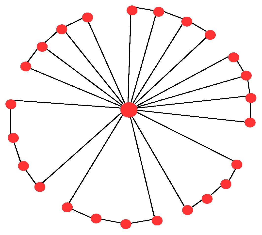
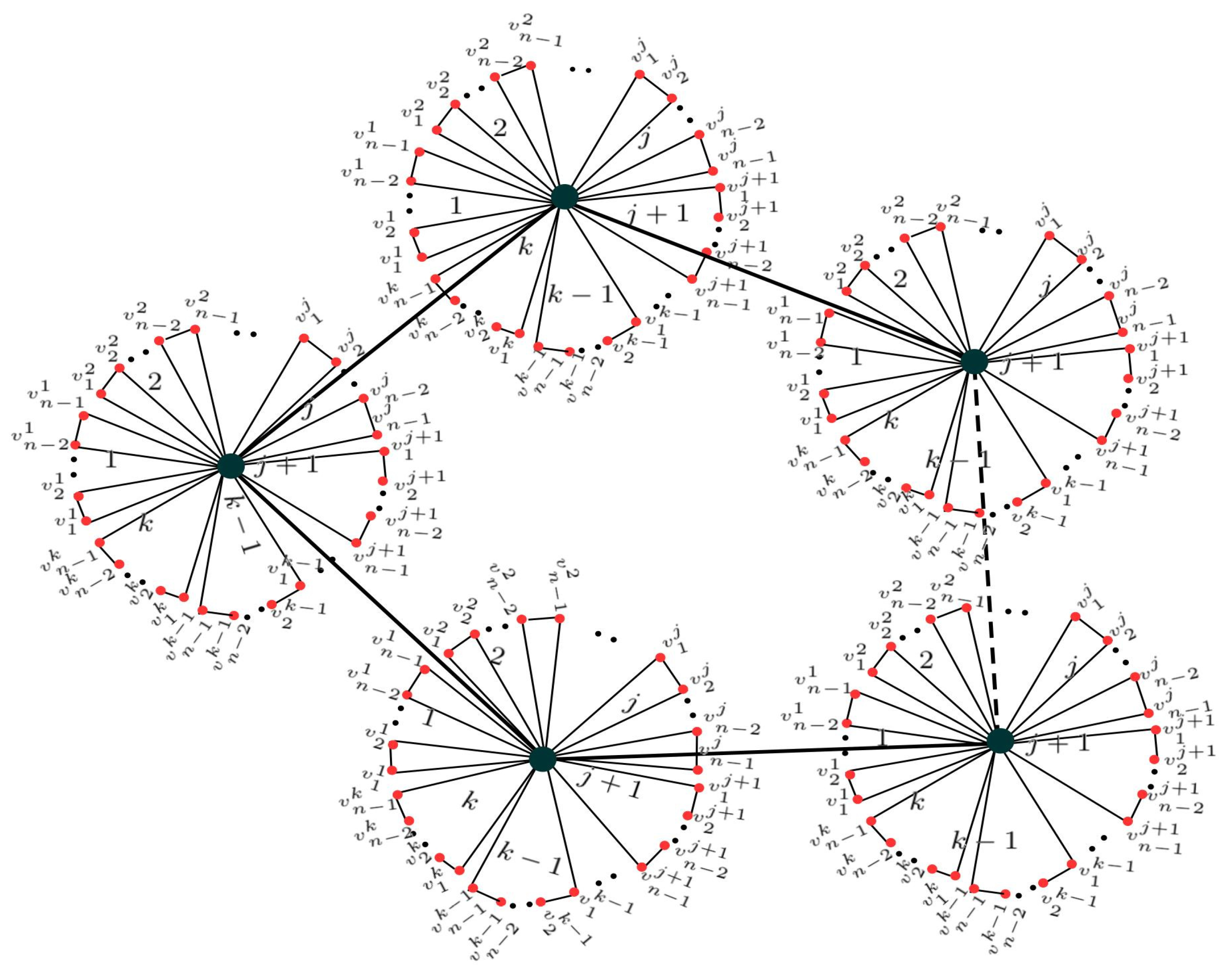
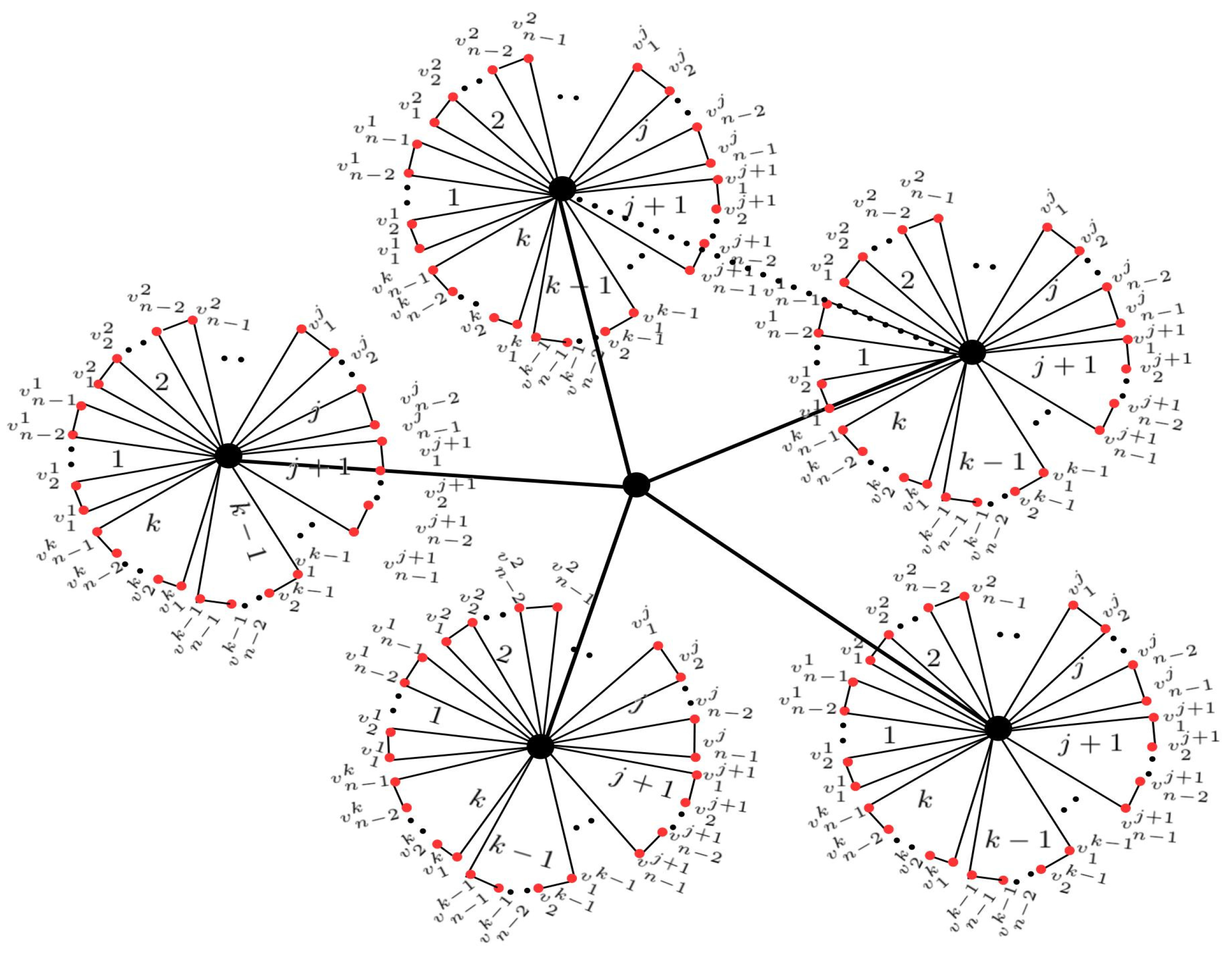
Definition 5.

Consider the cycle graph $C_n$ with $k\ge 2$ copies, where each copy has a common vertex known as the central vertex. In j copies of the cycle graph, we add an edge between the central vertex and each vertex that is not adjacent to it, where $1\le j\le k$. This results in the flabellum graph $F_n^{(k,j)}$, which can be seen in Figure 1. The order and size of the flabellum graph are $k(n-1)+1$ and $kn+(n-3)j$, respectively. For $n=3$, the flabellum graph $F_3^{(k,j)}$ is isomorphic to either the Dutch windmill graph $D_3^{\left(k\right)}$ or the friendship graph.

Theorem 1.

Let $F_5^{(k,\frac{k}{2})}$ be a graph, then

$$E(F_5^{(k,\frac{k}{2})})=(2k+1)\sqrt{5}+|\frac{1+\sqrt{5+12k}}{2}|+|\frac{1-\sqrt{5+12k}}{2}|.$$

Proof. 

Since the adjacency matrix of the graph $F_5^{(k,\frac{k}{2})}$ is symmetric, it can be written in the block form as follows:

$$A(F_5^{(k,\frac{k}{2})})=\left[\begin{array}{cccc}0& {\mathbb{1}}_{2k}^t& {\mathbb{1}}_k^t& {\mathbf{0}}_k^t\\ {\mathbb{1}}_{2k}& I_{\frac{k}{2}}\otimes A\left(P_4\right)& O_{2k,k}& O_{2k,k}\\ {\mathbb{1}}_k& O_{k,2k}& O_{k,k}& I_k\\ {\mathbf{0}}_k& O_{k,2k}& I_k& I_{\frac{k}{2}}\otimes A\left(P_2\right)\end{array}\right].$$

Then

$$\begin{array}{ll}f(F_5^{(k,\frac{k}{2})};x)& =\det \left(xI-A(F_5^{(k,\frac{k}{2})})\right)\\ & =\det \left(\left[\begin{array}{cccc}x& -{\mathbb{1}}_{2k}^t& -{\mathbb{1}}_k^t& {\mathbf{0}}_k^t\\ -{\mathbb{1}}_{2k}& I_{\frac{k}{2}}\otimes (x{I}_4-A\left(P_4\right))& O_{2k,k}& O_{2k,k}\\ -{\mathbb{1}}_k& O_{k,2k}& x{I}_k& -I_k\\ {\mathbf{0}}_k& O_{k,2k}& -I_k& I_{\frac{k}{2}}\otimes (x{I}_2-A\left(P_2\right))\end{array}\right]\right),\end{array}$$

by Lemma 3, we obtain

$$\begin{array}{l}=\det \left(I_{\frac{k}{2}}\otimes (x{I}_2-A\left(P_2\right))\right)\det \left(\left[\begin{array}{ccc}x& -{\mathbb{1}}_{2k}^t& -{\mathbb{1}}_k^t\\ -{\mathbb{1}}_{2k}& I_{\frac{k}{2}}\otimes (x{I}_4-A\left(P_4\right))& O_{2k,k}\\ -{\mathbb{1}}_k& O_{k,2k}& x{I}_k\end{array}\right]\right.\\ -\left[\begin{array}{c}{\mathbf{0}}_k^t\\ O_{2k,k}\\ -I_k\end{array}\right]{\left(I_{\frac{k}{2}}\otimes (x{I}_2-A\left(P_2\right))\right)}^{-1}\left.{\left[\begin{array}{c}{\mathbf{0}}_k^t\\ O_{2k,k}\\ -I_k\end{array}\right]}^t\right)\\ ={\left(f(P_2;x)\right)}^{\frac{k}{2}}det\left(\left[\begin{array}{ccc}x& -{\mathbb{1}}_{2k}^t& -{\mathbb{1}}_k^t\\ -{\mathbb{1}}_{2k}& I_{\frac{k}{2}}\otimes (x{I}_4-A\left(P_4\right))& O_{2k,k}\\ -{\mathbb{1}}_k& O_{k,2k}& x{I}_k\end{array}\right]\right.\\ -\left.\left[\begin{array}{cc}{O}_{2k+1,2k+1}& O_{2k+1,k}\\ O_{k,2k+1}& c_1{\mathcal{B}}_{k,k}\end{array}\right]\right),\end{array}$$

where $c_1=\frac{1}{x^2-1}$, $\mathcal{B}={\left[\begin{array}{ccccc}F& O& O& \cdots & O\\ O& F& O& \cdots & O\\ ⋮& ⋮& ⋮& \ddots & ⋮\\ O& O& O& \cdots & F\end{array}\right]}_{k,k}$ and $F=\left[\begin{array}{cc}x& 1\\ 1& x\end{array}\right].$

Then

$$\begin{array}{ll}f(F_5^{(k,\frac{k}{2})};x)& ={\left(f(P_2;x)\right)}^{\frac{k}{2}}\det \left(\left[\begin{array}{ccc}x& -{\mathbb{1}}_{2k}^t& -{\mathbb{1}}_k^t\\ -{\mathbb{1}}_{2k}& I_{\frac{k}{2}}\otimes (x{I}_4-A\left(P_4\right))& O_{2k,k}\\ -{\mathbb{1}}_k& O_{k,2k}& x{I}_k-c_1{\mathcal{B}}_{k,k}\end{array}\right]\right)\\ & ={\left(x^2-1\right)}^{\frac{k}{2}}\det (x{I}_k-c_1{\mathcal{B}}_{k,k})\det \left(\left[\begin{array}{cc}x& -{\mathbb{1}}_{2k}^t\\ -{\mathbb{1}}_{2k}& I_{\frac{k}{2}}\otimes (x{I}_4-A\left(P_4\right))\end{array}\right]\right.\\ & -\left.\left[\begin{array}{c}-{\mathbb{1}}_k^t\\ O_{2k,k}\end{array}\right]{\left(x{I}_k-c_1{\mathcal{B}}_{k,k}\right)}^{-1}\left[\begin{array}{cc}-{\mathbb{1}}_k& O_{k,2k}\end{array}\right]\right)\\ & ={\left(x^2-1\right)}^{\frac{k}{2}}\det (x{I}_k-c_1{\mathcal{B}}_{k,k})\det \left(\left[\begin{array}{cc}x& -{\mathbb{1}}_{2k}^t\\ -{\mathbb{1}}_{2k}& I_{\frac{k}{2}}\otimes (x{I}_4-A\left(P_4\right))\end{array}\right]\right.\\ & -c_2\left.{\left[\begin{array}{cccc}1& 0& \cdots & 0\\ 0& 0& \cdots & 0\\ ⋮& ⋮& \ddots & ⋮\\ 0& 0& \cdots & 0\end{array}\right]}_{2k+1,2k+1}\right),\mathrm{where}{c}_2=\frac{k(x-1)}{x^2-x-1},\\ & ={\left(x^2-1\right)}^{\frac{k}{2}}\det (x{I}_k-c_1{\mathcal{B}}_{k,k})\det \left(\left[\begin{array}{cc}x-c_2& -{\mathbb{1}}_{2k}^t\\ -{\mathbb{1}}_{2k}& I_{\frac{k}{2}}\otimes (x{I}_4-A\left(P_4\right))\end{array}\right]\right)\\ & ={\left(x^2-1\right)}^{\frac{k}{2}}{\left(f(P_4;x)\right)}^{\frac{k}{2}}\det (x{I}_k-c_1{\mathcal{B}}_{k,k})\det \left(x-c_2\right)\\ & -\left.{\mathbb{1}}_{2k}^t{\left(I_{\frac{k}{2}}\otimes (x{I}_4-A\left(P_4\right))\right)}^{-1}{\mathbb{1}}_{2k}\right)\\ & ={\left(x^2-1\right)}^{\frac{k}{2}}{\left(x^4-3x^2+1\right)}^{\frac{k}{2}}{\left(\frac{x^4-3x^2+1}{x^2-1}\right)}^{\frac{k}{2}}\left(x-c_2-c_3\right),\\ & \mathrm{where}{c}_3=\frac{k(2x+1)}{x^2-x-1},\\ & ={\left(x^4-3x^2+1\right)}^k\left(\frac{x(x^2-x-3k-1))}{x^2-x-1}\right)\\ & =x{(x^2+x-1)}^k{(x^2-x-1)}^{k-1}(x^2-x-3k-1).\end{array}$$

Then

$$\begin{array}{ll}E(F_5^{(k,\frac{k}{2})})& =1\times \left|0\right|+(k-1)\times |\frac{1+\sqrt{5}}{2}|+(k-1)\times |\frac{1-\sqrt{5}}{2}|+k\times |\frac{-1+\sqrt{5}}{2}|+k\times |\frac{-1-\sqrt{5}}{2}|\\ & +1\times |\frac{1+\sqrt{5+12k}}{2}|+1\times |\frac{1-\sqrt{5+12k}}{2}|\\ & =(2k-1)\sqrt{5}+|\frac{1+\sqrt{5+12k}}{2}|+|\frac{1-\sqrt{5+12k}}{2}|.\end{array}$$

□

Remark 2.

$F_5^{(k,\frac{k}{2})}$ is very close to satisfying property $(-SR)$.

Example 1.

The graph $F_5^{(6,3)}$ shown in Figure 2 is very close to satisfying the property $(-SR)$. Here, $\sigma \left(F_5^{(6,3)}\right)=\{(0,1),(\frac{1\pm \sqrt{5}}{2},5),(\frac{-1\pm \sqrt{5}}{2},6),(\frac{1\pm \sqrt{77}}{2},1)\}$. Then $E\left(F_5^{(6,3)}\right)=33.371.$

We will now define some generalized flabellum graphs, namely the flabellum complete graph, flabellum cycle graph, and flabellum star graph.

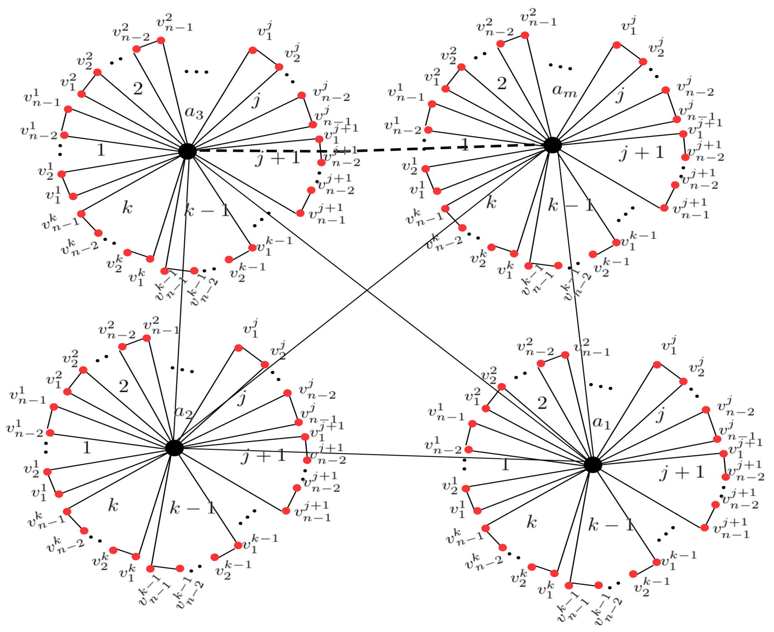
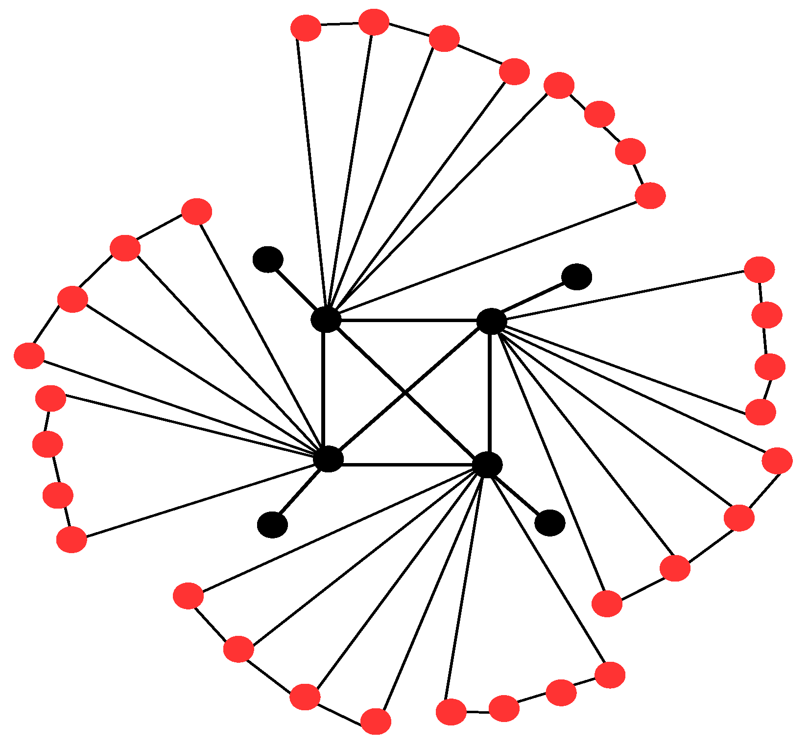
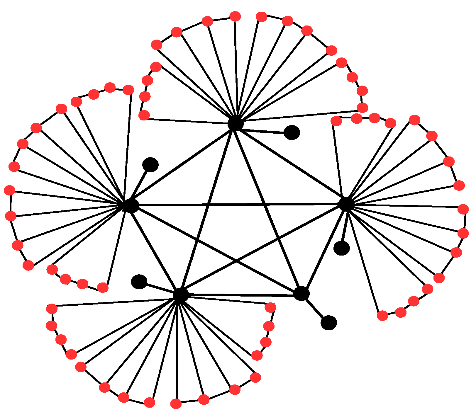
Definition 6.

Consider a complete graph $K_m$ and m copies of the flabellum graph $F_n^{(k,j)}$. The flabellum complete graph $K_m{F}_n^{(k,j)}$ can be obtained by attaching a copy of the flabellum graph $F_n^{(k,j)}$ to each vertex of the complete graph $K_m$, as shown in Figure 3.

Now, with the help of the flabellum complete graph $K_m{F}_n^{(k,j)},$ we construct four different types of families of $(-SR)$ graphs, namely, ${\mathcal{KF}}^1$, ${\mathcal{KF}}^2$, ${\mathcal{KF}}^3$, and ${\mathcal{KF}}^4$.

Family ${\mathcal{KF}}^1$

Consider the flabellum complete graph $K_m{F}_5^{(2,1)}$. The graph ${\Theta }_m^1=K_m^{*}{F}_5^{(2,1)}$ can be obtained by adding a pendant edge to each vertex of $K_m$. The family of all such graphs is denoted by ${\mathcal{KF}}^1$ and

$${\mathcal{KF}}^1=\{{\Theta }_m^1:m\in {\mathbb{Z}}^{+}\}.$$

In the following theorem, it is established that each graph in the family ${\mathcal{KF}}^1$ is a $\left(-SR\right)$ graph.

Theorem 2.

Let ${\Theta }_m^1\in {\mathcal{KF}}^1$, then ${\Theta }_m^1$ is a ($-SR$) graph.

Proof. 

Let ${\Theta }_m^1\in {\mathcal{KF}}^1$, then ${\Theta }_m^1=K_m^{*}{F}_5^{(2,1)}$. The adjacency matrix of ${\Theta }_m^1$ can be written as:

$$A\left({\Theta }_m^1\right)=\left[\begin{array}{cc}A(K_m\circ K_1)& \mathcal{M}\otimes {\mathcal{U}}^t\\ {\mathcal{M}}^t\otimes \mathcal{U}& I_{2m}\otimes A\left(P_4\right)\end{array}\right],$$

where

$$\mathcal{U}=\left[\begin{array}{c}{\mathbb{1}}_6\\ 0\\ 0\end{array}\right]$$

and

$$\mathcal{M}=\left[\begin{array}{c}{\mathbb{I}}_m\\ O_m\end{array}\right].$$

Then

$$\begin{array}{l}f({\Theta }_m^1;x)=\det \left(xI-A\left({\Theta }_m^1\right)\right)\\ =\det \left(\left[\begin{array}{cc}x{I}_{2m}-A(K_m\circ K_1)& -\mathcal{M}\otimes {\mathcal{U}}^t\\ -{\mathcal{M}}^t\otimes \mathcal{U}& I_{2m}\otimes (x{I}_4-A\left(P_4\right))\end{array}\right]\right),\end{array}$$

by Lemma 3, we obtain

$$\begin{array}{ll}=\det \left(I_{2m}\otimes (x{I}_4-A\left(P_4\right))\right)& \det \left(x{I}_{2m}-A(K_m\circ K_1)-\mathcal{M}\otimes {\mathcal{U}}^t{(I_{2m}\otimes (x{I}_4-A\left(P_4\right)))}^{-1}{\mathcal{M}}^t\otimes \mathcal{U}\right)\\ & ={\left(f(P_4;x)\right)}^{2m}det\left((x{I}_{2m}-A(K_m\circ K_1)+\left[\begin{array}{cc}c{I}_m& O_m\\ O_m& O_m\end{array}\right]\right),\end{array}$$

where $c=\frac{-6x}{x^2-x-1}$. Now, by using Lemma 2

$$\begin{array}{l}={\left(f(P_4;x)\right)}^{2m}[\det (x{I}_{2m}-A(K_m\circ K_1))+\left(\frac{-6x}{x^2-x-1}\right){\sum }_{i=1}^m\det (x{I}_{2m}-A(K_m\circ K_1)\left[i\right])\\ +{\left(\frac{-6x}{x^2-x-1}\right)}^2\left(\genfrac{}{}{0pt}{}{m}{2}\right){\sum }_{i,j=1}^m\det (x{I}_{2m}-A(K_m\circ K_1)[i,j])+\dots +{\left(\frac{-6x}{x^2-x-1}\right)}^m\left(\genfrac{}{}{0pt}{}{m}{m}\right)\det (x{I}_{2m}-A(K_m\circ K_1)[1,2,\dots ,m])]\\ =\frac{{\left(f(P_4;x)\right)}^{2m}}{{(x^2-x-1)}^m}[f_0\left(x\right)-6x^2{f}_1\left(x\right)+6^2{x}^4{f}_2\left(x\right)+\dots +{(-1)}^m{6}^m{x}^{2m}{f}_m\left(x\right)],\mathrm{where}\\ f_0\left(x\right)={(x^2-x-1)}^m\det (x{I}_{2m}-A(K_m\circ K_1)),\end{array}$$

and for $i=1,2,\dots ,m$

$$f_i\left(x\right)=\frac{{(x^2-x-1)}^{m-i}}{x^i}\sum _{\begin{array}{c}{t}_1,t_2,\dots ,t_i=1\\ t_1\le t_2\le \dots \le t_i\end{array}}^k\left(\genfrac{}{}{0pt}{}{m}{i}\right)\det (x{I}_{2m}-A(K_m\circ K_1))[t_1,t_2,\dots ,t_i].$$

Here, $\frac{{\left(f(P_4;x)\right)}^{2m}}{{(x^2-x-1)}^m}$ and $f_0\left(x\right)$ satisfy property $(-SR)$. Moreover, $\frac{\det (x{I}_{2m}-A(K_m\circ K_1))[t_1,t_2,\dots ,t_i]}{x_i}$ satisfies property $(-SR)$ for $i=1,2,\dots ,k$. Thus, the characteristic polynomial $f({\Theta }_m;x)$ satisfies property $(-SR)$ from Remark 1. Hence, graph ${\Theta }_m^1$ is a $(-SR)$ graph. □

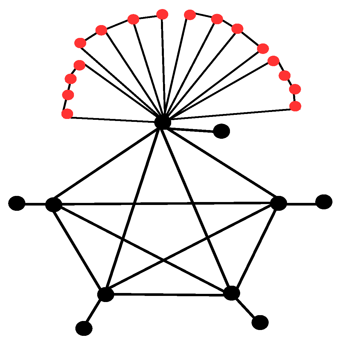
Example 2.

Let ${\Theta }_4^1=K_4^{*}{F}_5^{(2,1)}\in {\mathcal{KF}}^1$, as shown in Figure 4. Then

$$\sigma \left({\Theta }_4^1\right)=\left(\begin{array}{cccccc}-2.9811& -1.6180& -1.3737& -0.6180& -0.335& -0.2061\\ 3& 8& 1& 4& 3& 1\\ 0.3354& 0.6180& 0.7279& 1.6180& 2.9811& 4.8518\\ 3& 8& 1& 4& 3& 1\end{array}\right).$$

Therefore, graph ${\Theta }_4^1=K_4^{*}{F}_5^{(2,1)}$ is a $(-SR)$ graph.

Using the Laplace expansion, we have the following Lemma.

Lemma 5.

Let A be an $n\times n$ matrix, then for any constant c,

$$det\left(A+c{\left[\begin{array}{cccc}1& 0& \cdots & 0\\ 0& 0& \cdots & 0\\ ⋮& ⋮& \ddots & ⋮\\ 0& 0& \cdots & 0\end{array}\right]}_{n,n}\right)=det\left(A\right)+cdet\left(\left(A\right)\left[1\right]\right).$$

Here, $\left(A\right)\left[1\right]$ is the submatrix of A, obtained by deleting the first row and first column.

Family ${\mathcal{KF}}^2$:

Consider $K_m{F}_5^{(k,\frac{k}{2})}$, where k is an even integer, then the graph $K_m^{*}{F}_5^{(k,\frac{k}{2})}$ can be obtained by adding a pendant to each vertex of the complete graph $K_m$ of $K_m{F}_5^{(k,\frac{k}{2})}$. The graph ${\Theta }_m^2=K_m^{*;m-1}{F}_5^{(k,\frac{k}{2})}$ can be obtained by removing $m-1$ copies of the flabellum graph from vertices of $K_m^{*}{F}_5^{(k,\frac{k}{2})}$. The family of all such graphs is denoted by ${\mathcal{KF}}^2$. The following result shows that each graph in ${\mathcal{KF}}^2$ is a $\left(-SR\right)$ graph.

Theorem 3.

Let ${\Theta }_m^2\in {\mathcal{KF}}^2$. Then ${\Theta }_m^2$ is a ($-SR$) graph.

Proof. 

Let ${\Theta }_m^2\in {\mathcal{KF}}^2$, then ${\Theta }_m^2=K_m^{*;m-1}{F}_5^{(2,1)}$. The adjacency matrix of ${\Theta }_m^2$ can be written as:

$$A\left({\Theta }_m^2\right)=\left[\begin{array}{cccc}A(K_m\circ K_1)& {\mathcal{E}}_{2m,2k}& {\mathcal{E}}_{2m,k}& O_{2m,k}\\ {\mathcal{E}}_{2m,2k}^t& I_{\frac{k}{2}}\otimes A\left(P_4\right)& O_{2k,k}& O_{2k,k}\\ {\mathcal{E}}_{2m,k}^t& O_{k,2k}& O_{k,k}& I_k\\ O_{k,2m}& O_{k,2k}& I_k& I_{\frac{k}{2}}\otimes A\left(P_2\right)\end{array}\right],$$

where

$$\mathcal{E}=\left[\begin{array}{cccc}{e}_1& e_1& \cdots & e_1\end{array}\right].$$

Then

$$\begin{array}{l}f\left({\Theta }_m^2;x\right)=\det \left(xI-A\left({\Theta }_m^2\right)\right)\\ =\det \left(\left[\begin{array}{cccc}x{I}_{2m}-A(K_m\circ K_1)& -{\mathcal{E}}_{2m,2k}& -{\mathcal{E}}_{2m,k}& O_{2m,k}\\ -{\mathcal{E}}_{2m,2k}^t& I_{\frac{k}{2}}\otimes (x{I}_4-A\left(P_4\right))& O_{2k,k}& O_{2k,k}\\ -{\mathcal{E}}_{2m,k}^t& O_{k,2k}& x{I}_k& -I_k\\ O_{k,2m}& O_{k,2k}& -I_k& I_{\frac{k}{2}}\otimes (x{I}_2-A\left(P_2\right))\end{array}\right]\right),\end{array}$$

by Lemma 3, we obtain

$$\begin{array}{l}=\det \left(I_{\frac{k}{2}}\otimes (x{I}_2-A\left(P_2\right))\right)\det \left(\left[\begin{array}{ccc}x{I}_{2m}-A(K_m\circ K_1)& -{\mathcal{E}}_{2m,2k}& -{\mathcal{E}}_{2m,k}\\ -{\mathcal{E}}_{2m,2k}^t& I_{\frac{k}{2}}\otimes (x{I}_4-A\left(P_4\right))& O_{2k,k}\\ -{\mathcal{E}}_{2m,k}^t& O_{k,2k}& x{I}_k\end{array}\right]\right.\\ -\left[\begin{array}{c}{O}_{2m,k}\\ O_{2k,k}\\ -I_k\end{array}\right]{\left(I_{\frac{k}{2}}\otimes (x{I}_2-A\left(P_2\right))\right)}^{-1}\left.{\left[\begin{array}{c}{O}_{2m,k}\\ O_{2k,k}\\ -I_k\end{array}\right]}^t\right)\\ ={\left(f(P_2;x)\right)}^{\frac{k}{2}}\det \left(\left[\begin{array}{ccc}x{I}_{2m}-A(K_m\circ K_1)& -{\mathcal{E}}_{2m,2k}& -{\mathcal{E}}_{2m,k}\\ -{\mathcal{E}}_{2m,2k}^t& I_{\frac{k}{2}}\otimes (x{I}_4-A\left(P_4\right))& O_{2k,k}\\ -{\mathcal{E}}_{2m,k}^t& O_{k,2k}& x{I}_k\end{array}\right]\right.\\ -\left.\left[\begin{array}{cc}{O}_{2m+2k}& O_{2m+2k,k}\\ O_{k,2m+2k}& c{\mathcal{B}}_{k,k}\end{array}\right]\right),\end{array}$$

where $c=\frac{1}{x^2-1}$, $\mathcal{B}={\left[\begin{array}{ccccc}F& O& O& \cdots & O\\ O& F& O& \cdots & O\\ ⋮& ⋮& ⋮& \ddots & ⋮\\ O& O& O& \cdots & F\end{array}\right]}_{k,k}$ and $F=\left[\begin{array}{cc}x& 1\\ 1& x\end{array}\right].$

Then

$$\begin{array}{l}f\left({\Theta }_m^2;x\right)={\left(f(P_2;x)\right)}^{\frac{k}{2}}\det \left(\left[\begin{array}{ccc}x{I}_{2m}-A(K_m\circ K_1)& -{\mathcal{E}}_{2m,2k}& -{\mathcal{E}}_{2m,k}\\ -{\mathcal{E}}_{2m,2k}^t& I_{\frac{k}{2}}\otimes (x{I}_4-A\left(P_4\right))& O_{2k,k}\\ -{\mathcal{E}}_{2m,k}^t& O_{k,2k}& x{I}_k-c{\mathcal{B}}_{k,k}\end{array}\right]\right)\\ ={\left(x^2-1\right)}^{\frac{k}{2}}\det (x{I}_k-c{\mathcal{B}}_{k,k})\det \left(\left[\begin{array}{cc}x{I}_{2m}-A(K_m\circ K_1)& -{\mathcal{E}}_{2m,2k}\\ -{\mathcal{E}}_{2m,2k}^t& I_{\frac{k}{2}}\otimes (x{I}_4-A\left(P_4\right))\end{array}\right]\right.\\ -\left.\left[\begin{array}{c}-{\mathcal{E}}_{2m,k}\\ O_{2k,k}\end{array}\right]{\left(x{I}_k-c{\mathcal{B}}_{k,k}\right)}^{-1}{\left[\begin{array}{c}-{\mathcal{E}}_{2m,k}\\ O_{2k,k}\end{array}\right]}^t\right)\\ ={\left(x^2-1\right)}^{\frac{k}{2}}\det (x{I}_k-c{\mathcal{B}}_{k,k})\det \left(\left[\begin{array}{cc}x{I}_{2m}-A(K_m\circ K_1)& -{\mathcal{E}}_{2m,2k}\\ -{\mathcal{E}}_{2m,2k}^t& I_{\frac{k}{2}}\otimes (x{I}_4-A\left(P_4\right))\end{array}\right]\right.\\ +c_2\left.\left[\begin{array}{cccc}1& 0& \cdots & 0\\ 0& 0& \cdots & 0\\ ⋮& ⋮& \ddots & ⋮\\ 0& 0& \cdots & 0\end{array}\right]\right),\mathrm{where}{c}_2=-\frac{k(x-1)}{x^2-x-1}.\mathrm{Let}\mathcal{H}=\left[\begin{array}{cccc}1& 0& \cdots & 0\\ 0& 0& \cdots & 0\\ ⋮& ⋮& \ddots & ⋮\\ 0& 0& \cdots & 0\end{array}\right],\\ ={\left(x^2-1\right)}^{\frac{k}{2}}{\left(\frac{x^4-3x^2+1}{x^2-1}\right)}^{\frac{k}{2}}\det \left(\left[\begin{array}{cc}x{I}_{2m}-A(K_m\circ K_1)+c_2\mathcal{H}& -{\mathcal{E}}_{2m,2k}\\ -{\mathcal{E}}_{2m,2k}^t& I_{\frac{k}{2}}\otimes (x{I}_4-A\left(P_4\right))\end{array}\right]\right)\\ ={\left(x^4-3x^2+1\right)}^{\frac{k}{2}}{\left(f(P_4;x)\right)}^{\frac{k}{2}}\det \left(x{I}_{2m}-A(K_m\circ K_1)+c_2\mathcal{H}\right.\\ -\left.{\mathcal{E}}_{2m,2k}{(I_{\frac{k}{2}}\otimes (x{I}_4-A\left(P_4\right)))}^{-1}{\mathcal{E}}_{2m,2k}^t\right)\\ ={\left(x^4-3x^2+1\right)}^k\det \left(x{I}_{2m}-A(K_m\circ K_1)+c_2\mathcal{H}+c_3\mathcal{H}\right),\mathrm{where}{c}_3=-\frac{k(2x+1)}{x^2-x-1}.\\ \mathrm{Let}c=c_2+c_3,\mathrm{then}\\ ={\left(x^4-3x^2+1\right)}^k\det \left(x{I}_{2m}-A(K_m\circ K_1)+c\mathcal{H}\right),\\ \mathrm{for}\mathrm{Lemma}5,\\ ={\left(x^4-3x^2+1\right)}^k\left(\det (x{I}_{2m}-A(K_m\circ K_1))+c·x·\det (x{I}_{2(m-1)}-A(K_{m-1}\circ K_1))\right)\\ ={\left(x^4-3x^2+1\right)}^k\left(\det (x{I}_{2m}-A\left(K_m\right))-\frac{3k{x}^2}{x^2-x-1}\det (x{I}_{2(m-1)}-A\left(K_{m-1}\right))\right)\\ ={\left(x^4-3x^2+1\right)}^k\left(\frac{{(x^2+x-1)}^{m-2}(x^6-(m-1)x^5-3k{x}^4-4x^4+3(mk-2k+m-1)x^3+3k{x}^2+4x^2-mx+x-1)}{x^2-x-1}\right).\\ ={\left(x^2+x-1\right)}^{m+k-2}{\left(x^2-x-1\right)}^{k-1}\left(x^6-(m-1)x^5-3k{x}^4-4x^4+3(mk-2k+m-1)x^3+3k{x}^2+4x^2-mx+x-1\right).\end{array}$$

Hence, $f({\Theta }_m^2;x)$ satisfies property $(-SR)$. Consequently, graph ${\Theta }_m^2$ is a $(-SR)$ graph. □

Example 3.

Let ${\Theta }_5^2=K_5^{*;4}{F}_5^{(4,2)}\in {\mathcal{KF}}^2$, as shown in Figure 5. Then

$$\sigma \left({\Theta }_5^2\right)=\left(\begin{array}{ccccc}-3.6465& -1.6180& -0.6180& -0.3652& -0.1925\\ 1& 7& 3& 1& 1\\ 0.2742& 0.6180& 1.6180& 2.7375& 5.1925\\ 1& 7& 3& 1& 1\end{array}\right..$$

Therefore, graph ${\Theta }_5^2=K_5^{*;4}{F}_5^{(4,2)}$ is a $(-SR)$ graph.

The family of $(-SR)$ graphs ${\mathcal{KF}}^2$ can be generalized as follows.

Family ${\mathcal{KF}}^3$:

Again, consider the flabellum complete graph $K_m{F}_5^{(k,\frac{k}{2})}$ (here, k is an even integer) and let $K_m^{*}{F}_5^{(k,\frac{k}{2})}$ be the graph obtained by adding a pendant to each vertex of $K_m$ of $K_m{F}_5^{(k,\frac{k}{2})}$. The graph ${\Theta }_m^3=K_m^{*;m-k}{F}_5^{(k,\frac{k}{2})}$ can then be obtained by removing $1\le m-k\le m$ copies of the flabellum graph from vertices of $K_m^{*}{F}_5^{(k,\frac{k}{2})}$. The family of all such graphs is denoted by ${\mathcal{KF}}^3$. The following result shows that each graph in ${\mathcal{KF}}^3$ is a property $\left(-SR\right)$ graph.

Theorem 4.

Let ${\Theta }_m^3\in {\mathcal{KF}}^3$, then ${\Theta }_m^3$ is a ($-SR$) graph.

Proof. 

Let ${\Theta }_m^3\in {\mathcal{KF}}^3$, then ${\Theta }_m^3=K_m^{*;m-k}{F}_5^{(2,1)}$. The adjacency matrix of ${\Theta }_m^3$ can be written as:

$$A(\Theta )=\left[\begin{array}{cc}A(K_m\circ K_1)& \mathcal{M}\otimes V^t\\ {\mathcal{M}}^t\otimes V& I_k\otimes A\left(P_4\right)\end{array}\right],$$

where

$$\mathcal{V}=\left[\begin{array}{c}{\mathbb{1}}_6\\ 0\\ 0\end{array}\right],$$

and

$$\mathcal{M}=\left[\begin{array}{c}{\mathbb{I}}_j\\ O_{k,j}\end{array}\right].$$

Then

$$\begin{array}{l}f({\Theta }_m^3;x)=\det \left(xI-A\left({\Theta }_m^3\right)\right)\\ =\det \left(\left[\begin{array}{cc}x{I}_{2m}-A(K_m\circ K_1)& -\mathcal{M}\otimes V^t\\ -{\mathcal{M}}^t\otimes V& I_k\otimes (x{I}_4-A\left(P_4\right))\end{array}\right]\right),\end{array}$$

by Lemma 3, we obtain

$$\begin{array}{ll}=\det \left(I_k\otimes (x{I}_4-A\left(P_4\right))\right)& \det \left(x{I}_{2m}-A(K_m\circ K_1)-\mathcal{M}\otimes V^t(I_k\otimes {(x{I}_4-A\left(P_4\right))}^{-1}{\mathcal{M}}^t\otimes V\right)\\ & ={\left(f(P_4;x)\right)}^{k}det\left((x{I}_{2m}-A(K_m\circ K_1)+\left[\begin{array}{cc}c{I}_{j,j}& O_{j,2m-j}\\ O_{2m-j,j}& O_{2m-j,2m-j}\end{array}\right]\right),\end{array}$$

where $c=\frac{-6x}{x^2-x-1}$. Now, by using Lemma 2

$$\begin{array}{l}={\left(f(P_4;x)\right)}^k\left[\det \right(x{I}_{2m}-A(K_m\circ K_1))+\left(\frac{-6x}{x^2-x-1}\right){\sum }_{i=1}^j\det (x{I}_{2m}-A(K_m\circ K_1)\left[i\right])\\ +{\left(\frac{-6x}{x^2-x-1}\right)}^2\left(\genfrac{}{}{0pt}{}{j}{2}\right){\sum }_{i,l=1}^j\det (x{I}_{2m}-A(K_m\circ K_1)[i,l])+\dots +{\left(\frac{-6x}{x^2-x-1}\right)}^j\left(\genfrac{}{}{0pt}{}{j}{j}\right)\det (x{I}_{2m}-A(K_m\circ K_1)[1,2,\dots ,j])]\\ =\frac{{\left(f(P_4;x)\right)}^k}{{(x^2-x-1)}^j}[f_0\left(x\right)-6x^2{f}_1\left(x\right)+6^2{x}^4{f}_2\left(x\right)+\dots +{(-1)}^j{6}^j{x}^{2j}{f}_j\left(x\right)],\end{array}$$

where

$$f_0\left(x\right)={(x^2-x-1)}^j\det (x{I}_{2m}-A(K_m\circ K_1)),$$

and for $i=1,2,\dots ,j$

$$f_i\left(x\right)=\frac{{(x^2-x-1)}^{j-i}}{x^i}\sum _{\begin{array}{c}{t}_1,t_2,\dots ,t_i=1\\ t_1\le t_2\le \dots \le t_i\end{array}}^k\left(\genfrac{}{}{0pt}{}{j}{i}\right)\det (x{I}_{2m}-A(K_m\circ K_1))[t_1,t_2,\dots ,t_i].$$

Notice that $\frac{{\left(f(P_4;x)\right)}^k}{{(x^2-x-1)}^j}$ and $f_0\left(x\right)$ satisfy property $(-SR)$. Moreover, $\frac{\det (x{I}_{2m}-A(K_m\circ K_1))[t_1,t_2,\dots ,t_i]}{x_i}$ satisfies property $(-SR)$ for $i=1,2,\dots ,k$. Therefore, according to Remark 1, the polynomial $f({\Theta }_m^3;x)$ satisfies property $(-SR)$. Hence, graph ${\Theta }_m^3$ is a $(-SR)$ graph. □

Example 4.

Let ${\Theta }_5^3=K_5^{*;1}{F}_5^{(4,2)}\in {\mathcal{KF}}^3$, as shown in Figure 6. Then

$$\sigma \left({\Theta }_5^2\right)=\left(\begin{array}{ccccc}-6.8176& -1.6180& -0.6180& -0.3177& -0.1255\\ 1& 19& 15& 1& 1\\ 0.1466& 0.6180& 1.6180& 3.1469& 7.9673\\ \\ 1& 19& 15& 1& 1\end{array}\right..$$

Hence, graph ${\Theta }_5^3=K_5^{*;1}{F}_5^{(4,2)}$ is a $(-SR)$ graph.

The family ${\mathcal{KF}}^3$ of $(-SR)$ graphs can be generalized as follows.

Family ${\mathcal{KF}}^4$:

Consider $K_m^{*}{F}_5^{(k,\frac{k}{2})}$, which is the graph obtained by adding a pendant to each vertex of $K_m$ of $K_m{F}_5^{(k,\frac{k}{2})}$. The graph $K_m^{*;m-\nu }{F}_5^{(k,\frac{k}{2})}$ can then be obtained by removing $\nu \le m$ copies of the flabellum graph from vertices of $K_m^{*}{F}_5^{(k,\frac{k}{2})}$, where $\nu$ is any positive integer. The family of these graphs is denoted by ${\mathcal{KF}}^4$. We present the following theorem, which can be proven using similar steps as in the proofs of previous theorems.

Theorem 5.

Let $K_m^{*;m-\nu }{F}_5^{(k,\frac{k}{2})}\in {\mathcal{KF}}^4$ then $K_m^{*;m-\nu }{F}_5^{(k,\frac{k}{2})}$ is a ($-SR$) graph.

Definition 7.

Consider a cycle graph $C_m$ and m copies of the flabellum graph $F_n^{(k,j)}$. The flabellum cycle graph $C_m{F}_n^{(k,j)}$ can be obtained by attaching a copy of the flabellum graph $F_n^{(k,j)}$ to each vertex of the cycle graph $C_m$, as shown in Figure 7.

Now, with the help of the flabellum cycle graph $C_m{F}_n^{(k,j)}$, we construct different families of strong anti-reciprocal graphs, namely, ${\mathcal{CF}}^1$, ${\mathcal{CF}}^2$, ${\mathcal{CF}}^3$, and ${\mathcal{CF}}^4$, which are defined as follows:

Family ${\mathcal{CF}}^1$:

Consider the flabellum cycle graph $C_m{F}_5^{(2,1)}$. The graph ${\Gamma }_m^1=C_m^{*}{F}_5^{(2,1)}$ can be obtained by adding a pendant edge to each vertex of $C_m$ and the family of all such graphs is denoted by ${\mathcal{CF}}^1$ and

$${\mathcal{CF}}^1=\{{\Gamma }_m^1:m\in {\mathbb{Z}}^{+}\}.$$

Family ${\mathcal{CF}}^2$:

Consider $C_m{F}_5^{(k,\frac{k}{2})}$, where k is an even integer, then the graph $C_m^{*}{F}_5^{(k,\frac{k}{2})}$ can be obtained by adding a pendant to each vertex of the cycle graph $C_m$ of $C_m{F}_5^{(k,\frac{k}{2})}$. The graph ${\Gamma }_m^2=C_m^{*;m-1}{F}_5^{(k,\frac{k}{2})}$ can be obtained by removing $m-1$ copies of the flabellum graph from vertices of $C_m^{*}{F}_5^{(k,\frac{k}{2})}$. The family of all such graphs is denoted by ${\mathcal{CF}}^2$ and

$${\mathcal{CF}}^2=\{{\Gamma }_m^2:m\in {\mathbb{Z}}^{+}\}.$$

Family ${\mathcal{CF}}^3$:

Again, consider the flabellum cycle graph $C_m{F}_5^{(k,\frac{k}{2})}$ (here, k is an even integer), and let $C_m^{*}{F}_5^{(k,\frac{k}{2})}$ be the graph obtained by adding a pendant to each vertex of $C_m$ of $C_m{F}_5^{(k,\frac{k}{2})}$. The graph ${\Gamma }_m^3=C_m^{*;m-k}{F}_5^{(k,\frac{k}{2})}$ can then be obtained by removing $1\le m-k\le m$ copies of the flabellum graph from vertices of $C_m^{*}{F}_5^{(k,\frac{k}{2})}$. The family of all such graphs is denoted by ${\mathcal{CF}}^3$ and

$${\mathcal{CF}}^3=\{{\Gamma }_m^3:m\in {\mathbb{Z}}^{+}\}.$$

The proof of the following theorem is similar to the proofs of Theorems 2–4.

Theorem 6.

Let ${\Gamma }_m^G\in \{{\mathcal{CF}}^1\cup {\mathcal{CF}}^2\cup {\mathcal{CF}}^2\}$ then ${\Gamma }_m^1$ is a ($-SR$) graph.

The family ${\mathcal{CF}}^3$ can be generalized as follows.

Family ${\mathcal{CF}}^4$:

Consider $C_m^{*}{F}_5^{(k,\frac{k}{2})}$, which is the graph obtained by adding a pendant to each vertex of $C_m$ of $C_m{F}_5^{(k,\frac{k}{2})}$. The graph $C_m^{*;m-\nu }{F}_5^{(k,\frac{k}{2})}$ can then be obtained by removing $\nu \le m$ copies of the flabellum graph from vertices of $C_m^{*}{F}_5^{(k,\frac{k}{2})}$, where $\nu$ is any positive integer. The family of all such graphs is denoted by ${\mathcal{CF}}^4$. The following theorem shows that the family ${\mathcal{CF}}^4$ is a family of $(-SR)$ graphs.

Theorem 7.

Let $C_m^{*;m-\nu }{F}_5^{(k,\frac{k}{2})}\in {\mathcal{CF}}^4$, then $C_m^{*;m-\nu }{F}_5^{(k,\frac{k}{2})}$ is a ($-SR$) graph.

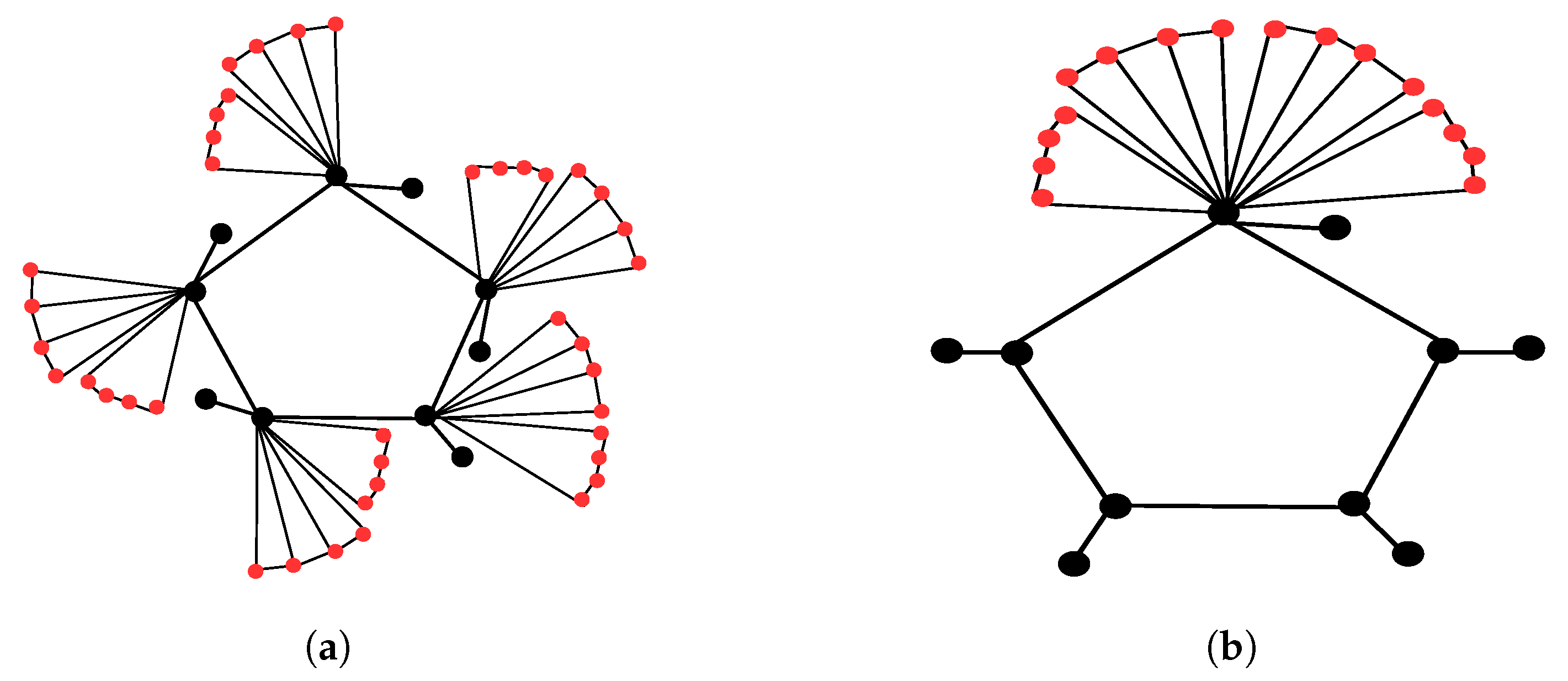
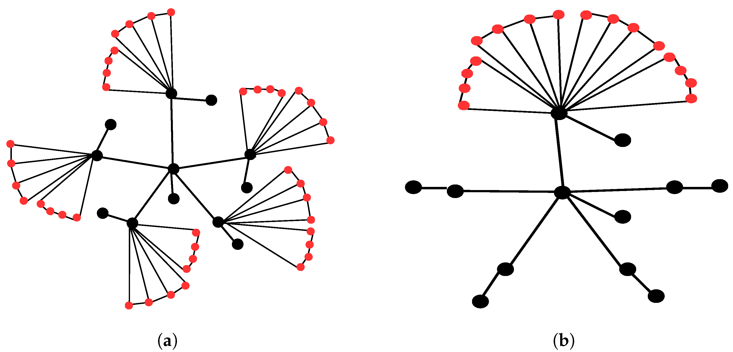
Example 5.

Let ${\Gamma }_5^1=C_5^{*}{F}_5^{(2,1)}\in {\mathcal{CF}}^1$, as shown in Figure 8a. Then

$$\sigma \left({\Gamma }_5^1\right)=\left(\begin{array}{ccccccc}-3.3820& -2.1196& -1.6180& -0.6180& -0.3542& -0.2818& -0.2360\\ 2& 2& 11& 5& 2& 2& 1\\ 0.2956& 0.4717& 0.6180& 1.6180& 2.8225& 3.5478& 4.2360\\ 2& 2& 11& 5& 2& 2& 1\end{array}\right).$$

Therefore, graph ${\Gamma }_5^1=C_5^{*}{F}_5^{(2,1)}$ is a $(-SR)$ graph.

Example 6.

Let ${\Gamma }_5^2=C_5^{*;4}{F}_5^{(4,2)}\in {\mathcal{CF}}^2$, as shown in Figure 8b. Then

$$\sigma \left({\Gamma }_5^2\right)=\left(\begin{array}{cccccccc}-3.6508& -2.0952& -1.6180& -1.2442& -0.7376& -0.6180& -0.4825& -0.2245\\ 1& 1& 4& 1& 1& 3& 1& 1\\ 0.2739& 0.4772& 0.6180& 0.8036& 1.3556& 1.6180& 2.0721& 4.4525\\ 1& 1& 4& 1& 1& 3& 1& 1\end{array}\right).$$

Therefore, graph ${\Gamma }_5^2=C_5^{*;4}{F}_5^{(4,2)}$ is a $(-SR)$ graph.

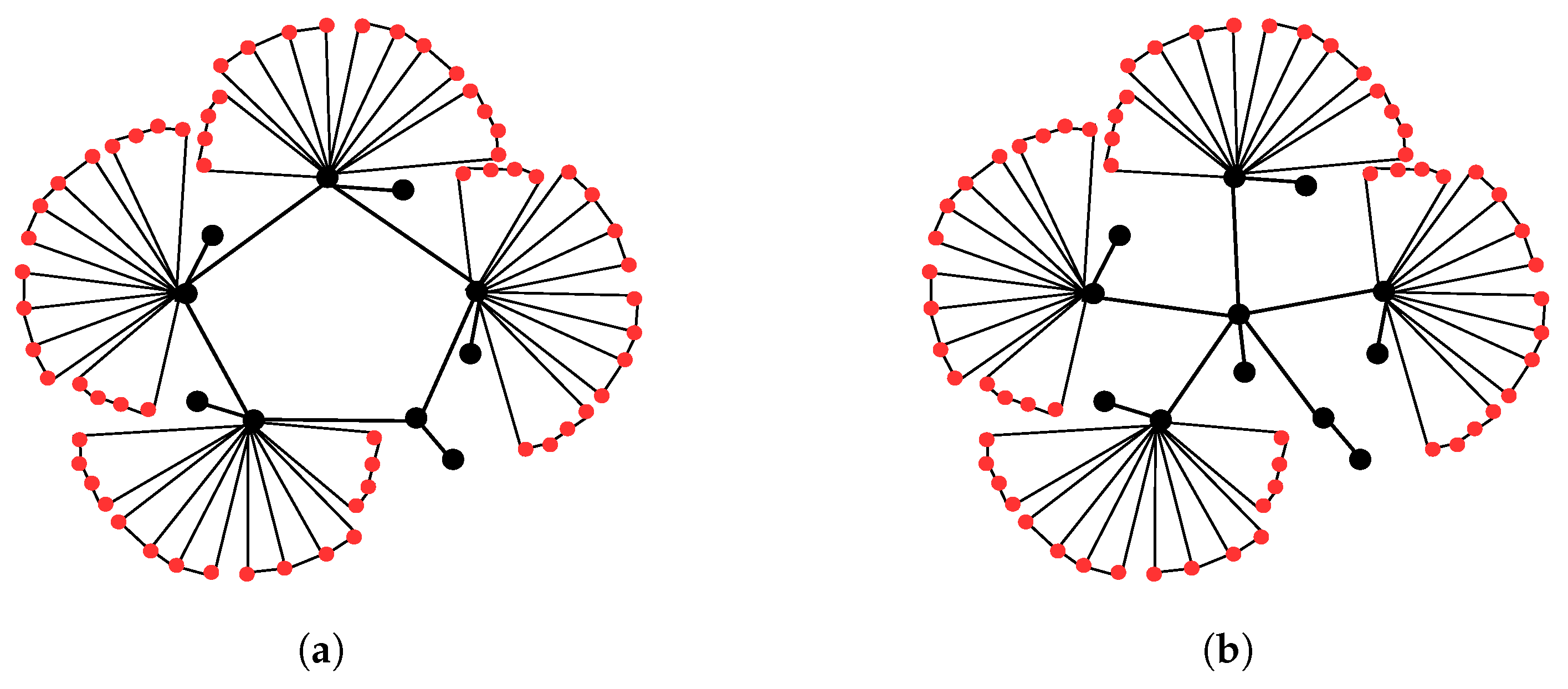
Example 7.

Let ${\Gamma }_5^3=C_5^{*;1}{F}_5^{(4,2)}\in {\mathcal{CF}}^3$, as shown in Figure 9a. Then

$$\sigma \left({\Gamma }_5^3\right)=\left(\begin{array}{cccccccc}-6.7612& -2.0952& -1.6180& -1.3249& -0.7376& -0.6180& -0.4785& -0.1298\\ 1& 1& 16& 1& 1& 15& 1& 1\\ 0.1479& 0.4772& 0.6180& 0.7547& 1.3556& 1.6180& 2.0894& 7.7024\\ 1& 1& 16& 1& 1& 15& 1& 1\end{array}\right).$$

Hence, this graph ${\Gamma }_5^3=C_5^{*;1}{F}_5^{(4,2)}$ is a $(-SR)$ graph.

Definition 8.

Consider a star graph $S_m$ and m copies of the flabellum graph $F_n^{(k,j)}$. The flabellum star graph $S_m{F}_n^{(k,j)}$ can be obtained by attaching a copy of the flabellum graph $F_n^{(k,j)}$ to each vertex of the star graph $S_m$, as shown in Figure 10.

Now, with the help of the flabellum star graph $S_m{F}_5^{(k,j)}$, we construct different families of strong anti-reciprocal graphs in the following definitions.

Family ${\mathcal{SF}}^1$:

Consider the flabellum star graph $S_m{F}_5^{(2,1)}$. The graph ${\Omega }_m^1=S_m^{*}{F}_5^{(2,1)}$ can be obtained by adding a pendant edge to each vertex of $S_m$ and the family of all such graphs is denoted by ${\mathcal{SF}}^1$ and

$${\mathcal{SF}}^1=\{{\Omega }_m^1:m\in {\mathbb{Z}}^{+}\}.$$

Family ${\mathcal{SF}}^2$:

Consider $S_m{F}_5^{(k,\frac{k}{2})}$, where k is an even integer, then the graph $S_m^{*}{F}_5^{(k,\frac{k}{2})}$ can be obtained by adding a pendant to each vertex of the star graph $S_m$ of $S_m{F}_5^{(k,\frac{k}{2})}$. The graph ${\Omega }_m^2=S_m^{*;m-1}{F}_5^{(k,\frac{k}{2})}$ can be obtained by removing $m-1$ copies of the flabellum graph from the vertices of $S_m^{*}{F}_5^{(k,\frac{k}{2})}$. The family of all such graphs is denoted by ${\mathcal{SF}}^2$ and

$${\mathcal{SF}}^2=\{{\Omega }_m^2:m\in {\mathbb{Z}}^{+}\}.$$

Family ${\mathcal{SF}}^3$:

Again, consider the flabellum star graph $S_m{F}_5^{(k,\frac{k}{2})}$ (here, k is an even integer), and let $S_m^{*}{F}_5^{(k,\frac{k}{2})}$ be the graph obtained by adding a pendant to each vertex of $S_m$ of $S_m{F}_5^{(k,\frac{k}{2})}$. The graph ${\Omega }_m^3=S_m^{*;m-k}{F}_5^{(k,\frac{k}{2})}$ can then be obtained by removing $1\le m-k\le m$ copies of the flabellum graph from vertices of $S_m^{*}{F}_5^{(k,\frac{k}{2})}$. The family of all such graphs is denoted by ${\mathcal{SF}}^3$ and

$${\mathcal{SF}}^3=\{{\Omega }_m^3:m\in {\mathbb{Z}}^{+}\}.$$

The following theorem, which can be proved in a similar way to the proofs of Theorems 2–4, reveals that the families ${\mathcal{SF}}^1$, ${\mathcal{SF}}^2$, and ${\mathcal{SF}}^3$ are families of $(-SR)$ graphs.

Theorem 8.

Let ${\Omega }_m^G\in \{{\mathcal{SF}}^1\cup {\mathcal{SF}}^2\cup {\mathcal{SF}}^3\}$, then ${\Omega }_m^G$ is a ($-SR$) graph.

Example 8.

Let ${\Omega }_5^1=S_5^{*}{F}_5^{(2,1)}\in {\mathcal{SF}}^1$, as shown in Figure 11a. Then

$$\sigma \left({\Omega }_5^1\right)=\left(\begin{array}{ccccccc}-3.3830& -2.4142& -1.6180& -0.8021& -0.6180& -0.3027& -0.2564\\ 1& 4& 10& 1& 5& 4& 1\\ 0.2955& 0.4142& 0.6180& 1.2466& 1.6180& 3.3027& 3.8992\\ 1& 4& 10& 1& 5& 4& 1\end{array}\right).$$

Therefore, graph ${\Omega }_5^1=S_5^{*}{F}_5^{(2,1)}$ is a $(-SR)$ graph.

Example 9.

Let ${\Omega }_5^2=S_5^{*;4}{F}_5^{(4,2)}\in {\mathcal{SF}}^2$, as shown in Figure 11b. Then

$$\sigma \left({\Omega }_5^2\right)=\left(\begin{array}{ccccccc}-3.5650& -2.2516& -1.6180& -1& -0.6180& -0.4211& -0.2289\\ 1& 1& 4& 3& 3& 1& 1\\ 0.2804& 0.4441& 0.6180& 1& 1.6180& 2.3746& 4.3675\\ 1& 1& 4& 3& 3& 1& 1\end{array}\right).$$

Therefore, graph ${\Gamma }_5^2=S_5^{*;4}{F}_5^{(4,2)}$ is a $(-SR)$ graph.

Example 10.

Let ${\Omega }_5^3=S_5^{*;1}{F}_5^{(4,2)}\in {\mathcal{SF}}^3$ as shown in Figure 9b. Then

$$\sigma \left({\Omega }_5^3\right)=\left(\begin{array}{ccccccc}-6.6867& -2.3845& -1.6180& -1& -0.6180& -0.4157& -0.1308\\ 1& 1& 16& 3& 15& 1& 1\\ 0.1495& 0.4193& 0.6180& 1& 1.6180& 2.4050& 7.6438\\ 1& 1& 16& 3& 15& 1& 1\end{array}\right).$$

Therefore, graph ${\Omega }_5^3=S_5^{*;1}{F}_5^{(4,2)}$ is a $(-SR)$ graph.

The family of $(-SR)$ graphs ${\mathcal{SF}}^3$ can be generalized as follows.

Family ${\mathcal{SF}}^4$:

Consider $S_m^{*}{F}_5^{(k,\frac{k}{2})}$, which is the graph obtained by adding a pendant edge to each vertex of $S_m$ in $S_m{F}_5^{(k,\frac{k}{2})}$. The graph $S_m^{*;m-\nu }{F}_5^{(k,\frac{k}{2})}$ can then be obtained by removing $\nu \le m$ copies of the flabellum graph from vertices of $S_m^{*}{F}_5^{(k,\frac{k}{2})}$, where $\nu$ is any positive integer. The family of all such graphs is denoted by ${\mathcal{SF}}^4$. We obtain the following theorem, which can be proved using similar steps as in the proofs of previous theorems.

Theorem 9.

Let $S_m^{*;m-\nu }{F}_5^{(k,\frac{k}{2})}\in {\mathcal{SF}}^4$ then $S_m^{*;m-\nu }{F}_5^{(k,\frac{k}{2})}$ is a ($-SR$) graph.

Remark 3.

All families can be generalized if we consider any connected graph instead of $K_m,C_m$, or $S_m$, and all of these generalized families are families of $(-SR)$ graphs.

3. Conclusions

In spectral graph theory, the reciprocal eigenvalue properties are of great interest. All corona graphs are $(-SR)$ graphs. The novelty of this research lies in introducing several families of graphs that satisfy property $(-SR)$. Some new families of graphs, denoted as the flabellum graph $F_n^{k,j}$, flabellum complete graph, flabellum cycle graph, and flabellum star graph, are introduced. Moreover, with the help of these families, several families of $(-SR)$ graphs are constructed. Furthermore, the energy of the flabellum graph $F_5^{k,\frac{k}{2}}$ is calculated.