Ordering Unicyclic Connected Graphs with Girth g ≥ 3 Having Greatest SK Indices

Abstract

For a graph, the SK index is equal to the half of the sum of the degrees of the vertices, the SK₁ index is equal to the half of the product of the degrees of the vertices, and the SK₂ index is equal to the half of the square of the sum of the degrees of the vertices. This paper shows a simple and unified approach to the greatest SK indices for unicyclic graphs by using some transformations and characterizes these graphs with the first, second, and third SK indices having order r ≥ 5 and girth g ≥ 3, where girth is the length of the shortest cycle in a graph.

1. Background Survey and Preliminary Results

In this paper, the term “graph” will always mean a simple, finite, and undirected graph. A graph [1] is an ordered pair $A=\left(V\right(A),E(A\left)\right)$ which is a representation of vertex set $V\left(A\right)$ and edge set $E\left(A\right)$. Here, $A$ is taken as a unicyclic connected graph having order $r$ and size $e$. Let the degree of a vertex $\omega$ be denoted by $d_A\left(\omega \right)$ whereas the distance between two vertices $\omega$ and $x$ be denoted by $d(\omega ,x)$. If $d\left(\omega \right)=1$ then $\omega$ is said to be a leaf or pendant vertex.

A graph invariant is a numerical parameter for the characterization of the topology of a graph which is calculated on the basis of a molecular graph of a chemical compound. Some invariants are degree based and some are based on distance.

For constructing relationships between the physical, chemical and biological characteristics and the arrangements of molecules in a chemical compound, the most useful tool is chemical invariants. These invariants are symmetric functions and provide us with a chance to examine or investigate the physical and chemical properties of molecules in a compound without the expenditure of money and time used in testing in a laboratory [2].

The most former topological index introduced by Harold Wiener is the Wiener index [3] which is expressed as

$$\mathrm{W}(\mathrm{A})=\sum _{\{\omega ,x\}\subseteq V(A)}{d}_A(\omega ,x)$$

(1)

i.e., the total of the distances between all of A’s unordered vertex pairs. Gutman and Trinajstić [4] established the first degree-based topological indices, the Zagreb indices, more than 30 years ago. Balaban et al. named them the Zagreb group indices after 10 years. It was later reduced to the Zagreb index [5,6].

The first Zagreb index and second Zagreb indexare defined as

$${\mathrm{M}}_1(A)=\sum _{\omega x\in E(A)}(d(\omega )+d(x))=\sum _{\omega \in V(A)}(d(\omega ){)}^2$$

(2)

$${\mathrm{M}}_2(A)=\sum _{\omega ,x\in E(A)}(d(\omega )d(x))$$

(3)

In 2016, Shigehalli and Kanabur [7] put forward the new degree-based graph invariants. These are presented as

$$\mathrm{S}\mathrm{K}(A)=\sum _{\omega x\in E(A)}\frac{d(\omega )+d(x)}{2}$$

(4)

$$\mathrm{S}{\mathrm{K}}_1(A)=\sum _{\omega x\in E(A)}\frac{d(\omega )d(x)}{2}$$

(5)

$$\mathrm{S}{\mathrm{K}}_2(A)=\sum _{\omega x\in E(A)}[\frac{d(\omega )+d(x)}{2}{]}^2$$

(6)

In the last 30 years, many researchers and scholars have been working on the chemical graph theory. Many authors worked on these connectivity indices.

Shigehalli et al. [7] computed SK indices of the $H$-naphtalenic nanotube and the $T\cup C_4[m,n]$ nanotube. In [8], Shigehalli et al. obtained the explicit formulas without the aid of a computer for the polyhex nanotube. In [9], $SK$ indices first appeared and also their explicit formula for Graphene was obtained. In [10], Shin Min Kang et al. calculated $SK$ and some other indices of Porphyrin, Zinc-Porphyrin, Propyl Ether Imine, and Poly Dendrimers and also plotted them using Maple software. In [11], Ranjini and Lokeshacalculated the $SK$ Indices of a graph operator subdivision graph $S(G)$ and semi-total point graph $R(G)$ on certain important chemical structures like tetracenic nanotubes and tetracenicnanotori. In [12], the behaviors of $SK,{SK}_1$ and ${SK}_2$ indices were investigated under some graphoperations by Nurkahli and Buyukkose. In [13], Roy and Ghosh concluded that the $ETA$ descriptors were sufficiently rich in chemical information to encode the structural features contributing to the toxicities and these indices might be used in combination with other topological and physicochemical descriptors for the development of predictive $QSAR$ models. Recently, Lokesha et al. [14] established the $SK$ indices of carbon nanocones using a $Q(A)$ operator. In [15], thegeneralized prism network of $SK$ indices was investigated. In [16], Harisha et al. calculated the SK indices of the semi-total point graph $R(G)$ and subdivision graph $S(G)$ on tetracenic nanotubes and tetracenicnanotori, two significant chemical structures. In [17], the behaviors of $SK$ indices were investigated under some graph operations when defined on weighted and interval weighted graphs.

1.1. Some Graph Transformations

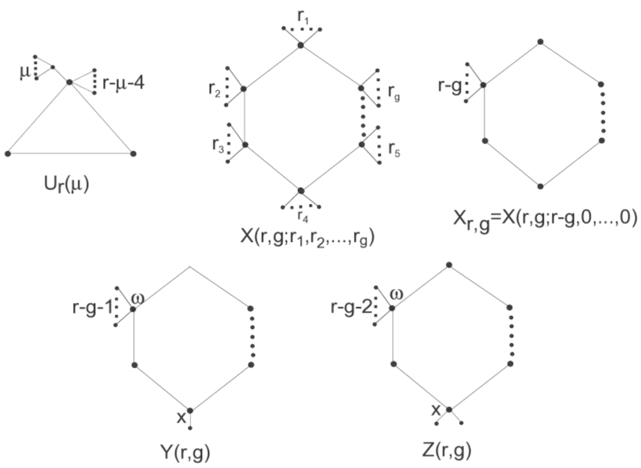
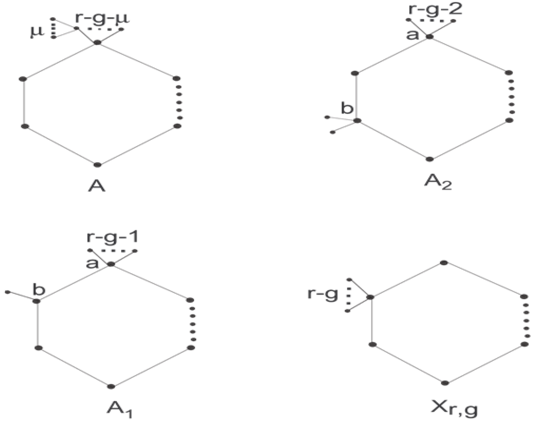
In $2014$, Tomescu et al. [18] used first and defined other three graph transformations to find the minimum, second and third minimum general sum connectivity indices of unicyclic connected graphs having fixed order and girth. These transformations are listed below.

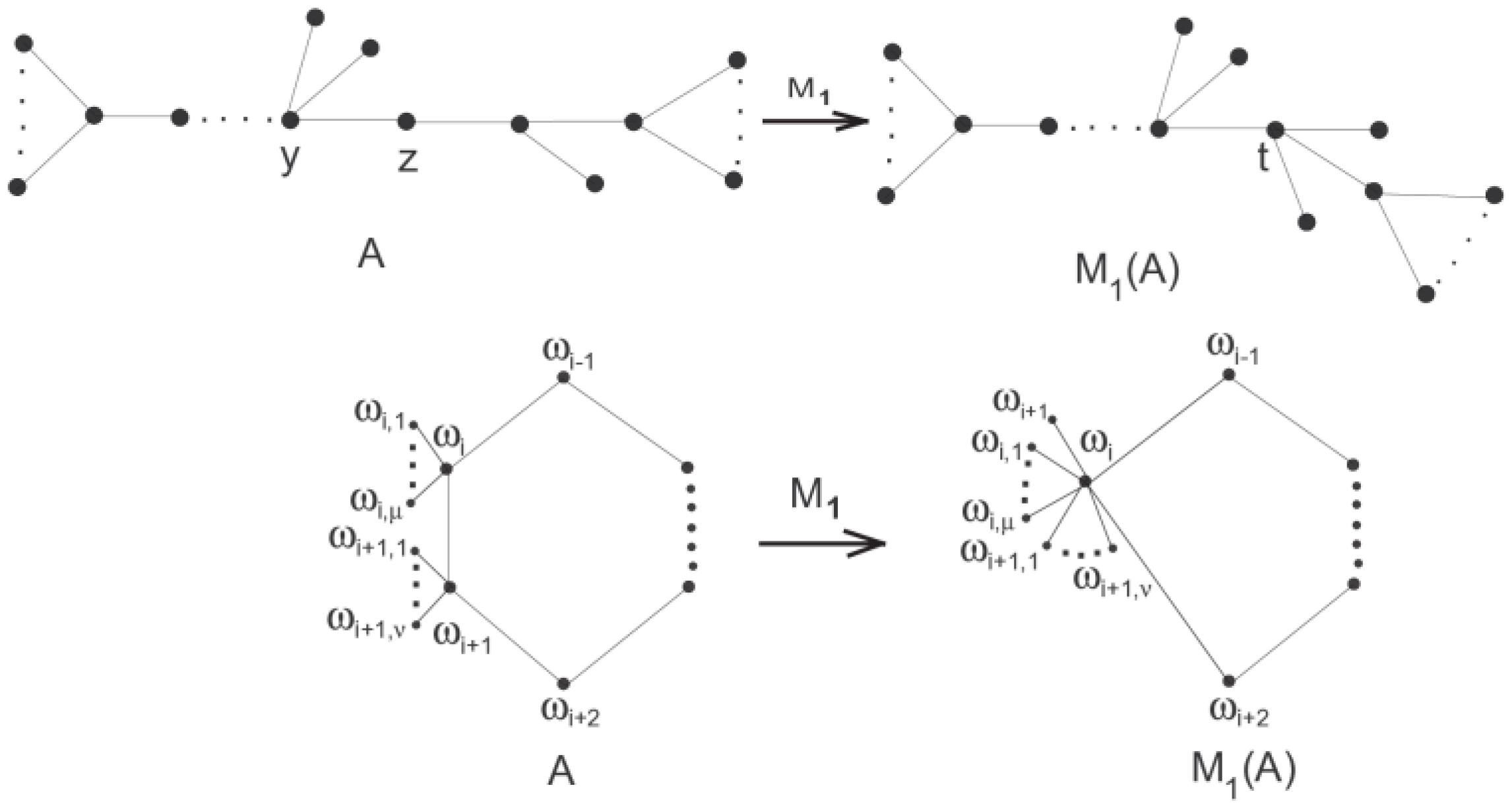
${\mathrm{M}}_1-\mathrm{t}\mathrm{r}\mathrm{a}\mathrm{n}\mathrm{s}\mathrm{f}\mathrm{o}\mathrm{r}\mathrm{m}\mathrm{a}\mathrm{t}\mathrm{i}\mathrm{o}\mathrm{n}$: In general, let $yz$ be an edge whose vertices $y$ and $z$ have no common neighbor in a connected graph, where $d\left(y\right),d(z)\ge 2$. Furthermore, let $M_1(A)$ be the graph obtained by deleting an edge $yz$, identifying $y$ and $z$ in a new vertex $t$ and adding a pendant edge to it.

In particular, let there be a connected unicyclic graph $A$ with two nearby vertices ${\omega }_i,{\omega }_{i+1}$ having no common neighbor in $A$, such that $\mu$ and $\nu$ pendant edges are linked to ${\omega }_i$ and ${\omega }_{i+1}$ with $d({\omega }_i)=\mu +2$ and $d({\omega }_{i+1})=\nu +2,$ respectively, where $d({\omega }_i,{\omega }_{i+1})\ge 2$. Then, the graph obtained by contracting edge ${\omega }_i{\omega }_{i+1}$ and attaching a new pendant edge to vertex ${\omega }_i$ is $M_1(A)$. (See Figure 1).

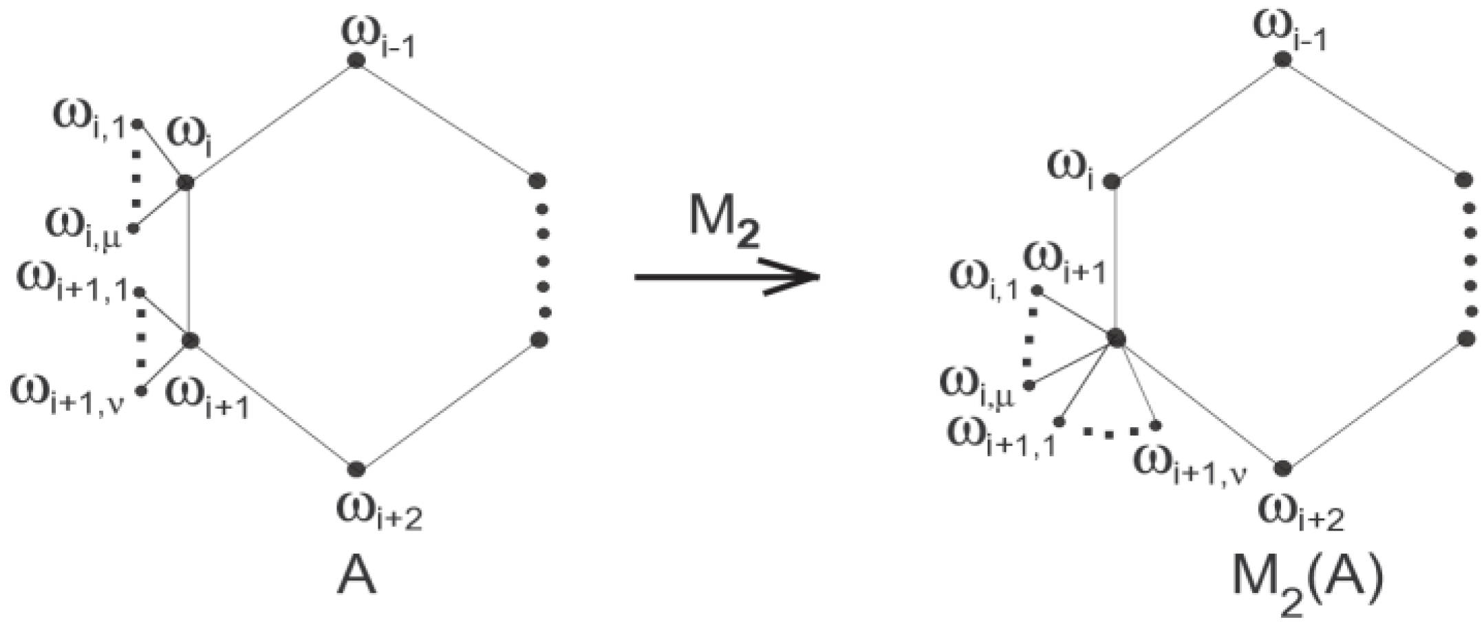
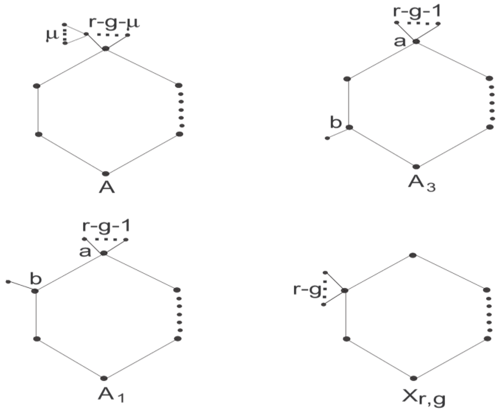
${\mathrm{M}}_2-\mathrm{t}\mathrm{r}\mathrm{a}\mathrm{n}\mathrm{s}\mathrm{f}\mathrm{o}\mathrm{r}\mathrm{m}\mathrm{a}\mathrm{t}\mathrm{i}\mathrm{o}\mathrm{n}$: Let ${\omega }_i,{\omega }_{i+1}$ be the neighboring vertices with pendant edges such that $d({\omega }_i)=\mu +2$, $d({\omega }_{i+1})=\nu +2$ in a connected unicyclic graph $A$ where $\mu ,\nu \ge 1$. Furthermore, after removing all the pendant edges incident to ${\omega }_i$ and attaching them to ${\omega }_{i+1}$, we obtained a graph $M_2(A)$ (see Figure 2).

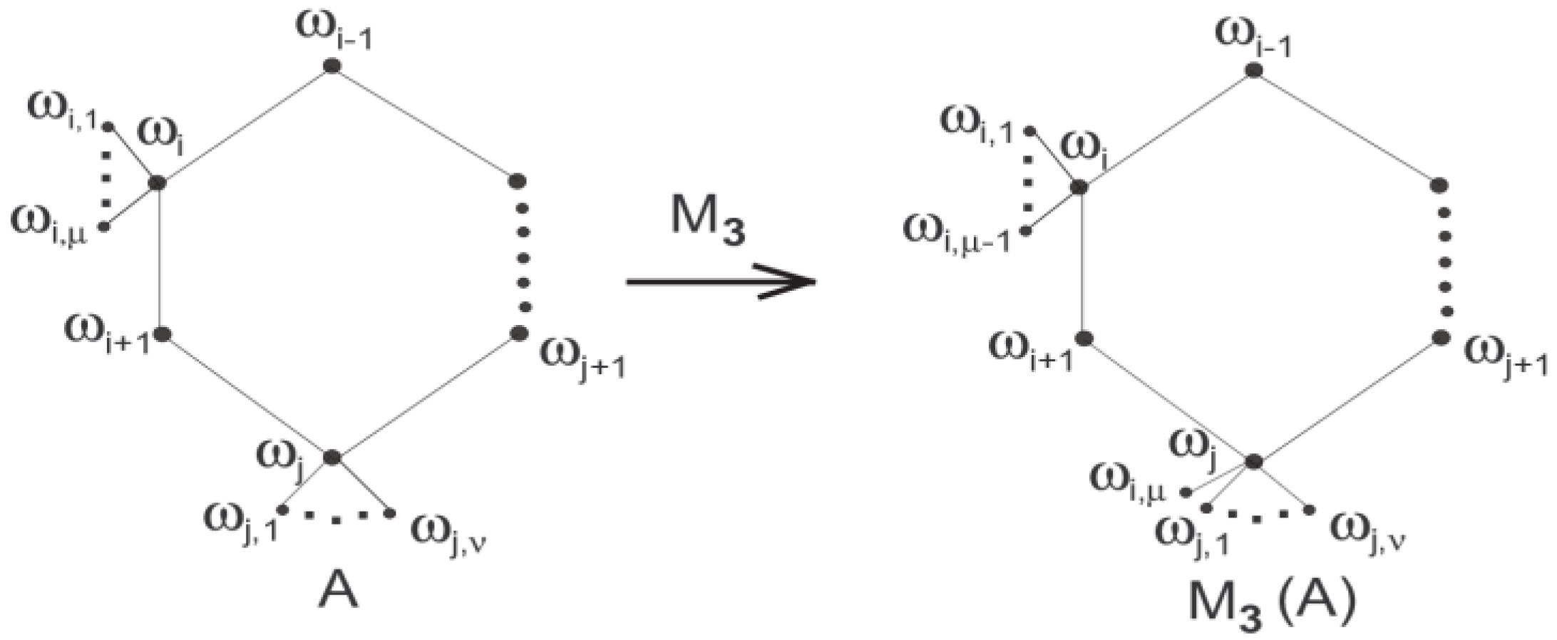
${\mathrm{M}}_3-\mathrm{t}\mathrm{r}\mathrm{a}\mathrm{n}\mathrm{s}\mathrm{f}\mathrm{o}\mathrm{r}\mathrm{m}\mathrm{a}\mathrm{t}\mathrm{i}\mathrm{o}\mathrm{n}$: Let $A$ be a unicyclic graph with vertices ${\omega }_i,{\omega }_j$ such that their distance $d({\omega }_i,{\omega }_j)\ge 2$ where $d({\omega }_i)=\mu +2$, $d({\omega }_j)=\nu +2$; $1\le \mu \le \nu$. Then, the graph we have after deleting one pendant edge from ${\omega }_i$ and adding it to ${\omega }_j$ is $M_3(A)$ (see Figure 3).

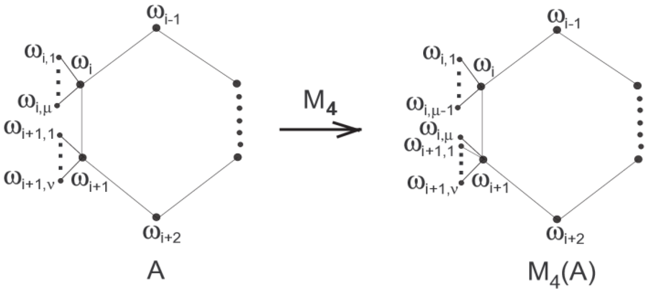
${\mathrm{M}}_4-\mathrm{t}\mathrm{r}\mathrm{a}\mathrm{n}\mathrm{s}\mathrm{f}\mathrm{o}\mathrm{r}\mathrm{m}\mathrm{a}\mathrm{t}\mathrm{i}\mathrm{o}\mathrm{n}$: Let ${\omega }_i,{\omega }_{i+1}$ be neighboring vertices of a unicyclic connected graph $A$ such that $d({\omega }_i)=\mu +2$, $d\left({\omega }_{i+1}\right)=\nu +2;1\le \mu \le \nu$. By $M_4-\mathrm{transformation}$, the graph $M_4(A)$ is attained by separating one pendant edge from ${\omega }_i$ and connecting it to ${\omega }_{i+1}$ (see Figure 4).

1.2. Certain Unicyclic Graphic Structures

Let a unicyclic graph $U_r(\mu )$ which is deduced from $X(r-\mu ,3;r-\mu -\mathrm{3,0},0)$ by adding $\mu$ pendant edges to a pendant vertex of it, where $1\le \mu \le r-4$.

Let the set of unlabelled connected unicyclic graphs be denoted by $O_{r,g}$ having order $r$ and girth $g$ where $r\ge g\ge 3$. A unicyclic graph $X(r,g;r_1,r_2,\dots ,r_g)$ with $r_i\ge 0$ is obtained by joining the $r_i$ pendant edges to a vertex ${\omega }_i;1\le i\le g$ of cycle $C_g={\omega }_1,{\omega }_2,\dots ,{\omega }_g,{\omega }_1$ where $r_1+r_2+\dots +r_g=r-g$. Moreover,$X_{r,g}=X\left(r,g;r-g,0,\dots ,0\right)$ (see Figure 5).

We will also use two sets of unicyclic connected graphs:

(i)

$Y(r,g)$ is the family of unicyclic graphs in which the $r-g-1$ pendant edges are incident to a vertex $\omega \in V(C_g)$ and one pendant edge to $x\in V(C_g)$, where $d(\omega ,x)\ge 2$.

(ii)

$Z(r,g)$ is the set of unicyclic graphs in which the $r-g-2$ pendant edges are incident to $\omega$ and two pendant edges are incident to $x$, where $d(\omega ,x)\ge 2$.

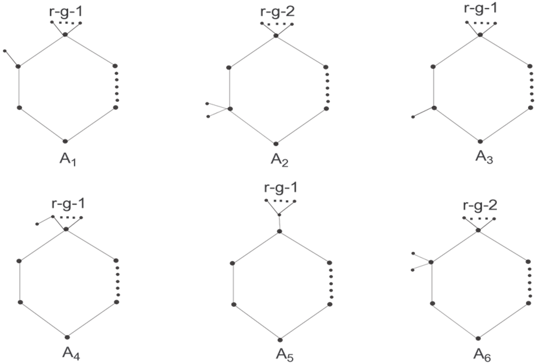
In $Y(r,g)$ and $Z(r,g)$, all graphs have similar index and properties. If $E\in Y_{r,g}$ and $F\in Z_{r,g}$ then $E=M_3(F)$. Moreover, we will utilize six different kinds of graphs to prove our main result, that are defined below:

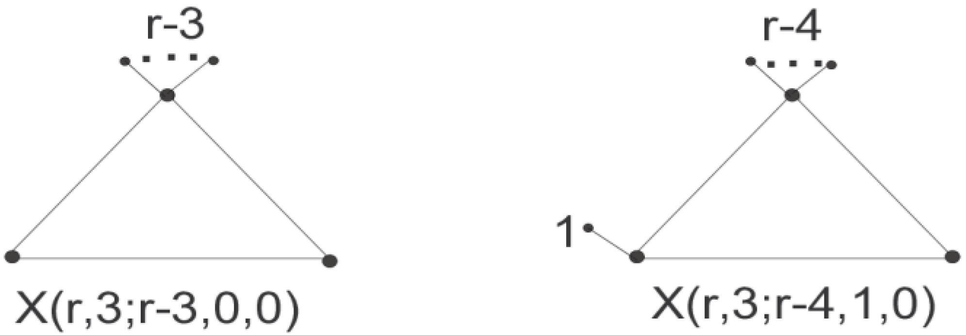
(i)

$A_1=X(r,g;\mu -\mathrm{1,1},0,\dots ,0)$ where $\mu =r-g\ge 2$.

(ii)

$A_2=X(r,g;\mu -\mathrm{2,0},\mathrm{2,0},\dots ,0)$ where $\mu =r-g\ge 2$. It can be easily seen that $A_2\in Z_{r,g}$.

(iii)

$A_3=X\left(r,g;\mu -\mathrm{1,0},\mathrm{1,0},\dots ,0\right).$

(iv)

$A_4$: It is deduced by attaching one pendant edge to a pendant vertex of $X(r-1,g;\mu -\mathrm{1,0},\dots ,0)$

(v)

$A_5$: It is obtained by connecting the $\mu -1$ pendant edges to the pendant vertex of $X(r-\mu +1,g;\mathrm{1,0},\dots ,0)$.

(vi)

$A_6=X\left(r,g;\mu -\mathrm{2,2},0,\dots ,0\right).$

(See Figure 6.)

In this paper, we study three maximum $SK$ indices, $\mathrm{i}.\mathrm{e}.,SK(A)$, $S{K}_1(A)$ and $S{K}_2(A)$ in a unicyclic connected graph $A$ having order $r\ge 5$ and girth $g\ge 3$.

2. Ordering Unicyclic Structures with the Greatest SK Index

In this section, we use some graph transformations which increase the $SK$ index.

Lemma 1.

Let $M_1(A)$ be a unicyclic connected graph as shown in Figure 1, then

$$SK(A)<SK(M_1(A))$$

for any $\mu ,v\ge 0$.

Proof. 

Case 1: Ref. [19] When $M_1$ is performed excluding the vertices of $C_g$

$$\begin{array}{ll}SK(A)-SK(M_1(A))& =\frac{1}{2}{\displaystyle \sum _{xy\in E(A)\backslash \{yz\}}}[(d_x+d_y)-(d_x+d_y+d_z-1)]\\ & +\frac{1}{2}{\displaystyle \sum _{xz\in E(A)\backslash \{yz\}}}[(d_x+d_z)-(d_x+d_y+d_z-1)]<0;as{d}_y\ge 2\end{array}$$

Case 2: When $M_1$ is performed on the vertices of $C_g$

We have $d_A({\omega }_i)=d_{M_1(A)}({\omega }_i)-v-1<d_{M_1(A)}({\omega }_i)$ and $d_{M_1(A)}({\omega }_i)+d_{M_1(A)}({\omega }_{i+1})=\mu +v+4$.

Therefore, for $j=\overline{1,\mu }=\mathrm{1,2},\dots ,\mu$, $k=\overline{1,v}=\mathrm{1,2},\dots ,v$ and by the definition of $SK$ index, we find

$$\begin{array}{ll}SK(A)-SK(M_1(A))& =\frac{1}{2}[\{d({\omega }_{i-1})+d({\omega }_i)\}+\mu \{d({\omega }_{i,j})+d({\omega }_i)\}+\{d({\omega }_i)\\ & +d({\omega }_{i+1})\}+\nu \{d({\omega }_{i+1,k})+d({\omega }_{i+1})\}+\{d({\omega }_{i+1})+d({\omega }_{i+2})\}]\\ & =\frac{1}{2}[\{d({\omega }_{i-1})+d({\omega }_i)\}+(\mu +\nu +1)\{d({\omega }_{i,l})+d({\omega }_i)\}\\ & \{d({\omega }_i)+d({\omega }_{i+2})\}]\\ & =-(\mu +\nu +\mu \nu +1)<0for\mu ,\nu \ge 0.\end{array}$$

$$\Rightarrow SK(A)<SK(M_1(A))\square$$

Lemma 2.

Let $M_2(A)$ be a unicyclic connected graph as depicted in Figure 2, where $d_A({\omega }_i,{\omega }_{i+1})=1$. Then

$$SK(A)<SK(M_2(A))$$

for any $v\ge \mu \ge 1$.

Proof. 

Since $d_{M_2(A)}({\omega }_i)=2<d_A({\omega }_i)=\mu +2$ and $d_A({\omega }_{i+1})=\nu +2<d_{M_2(A)}({\omega }_{i+1})=\nu +\mu +2$.

$$\begin{array}{ll}SK(A)-SK(M_2(A))& =\frac{1}{2}[\{d(u_{i-1})+d(u_i)\}+{\displaystyle \sum _{j=1}^{\mu }}\\ & \{d({\omega }_{i,j})+d({\omega }_i)\}+\{d({\omega }_i)+d({\omega }_{i+1})\}\\ & +{\displaystyle \sum _{k=1}^{\nu }}\{d({\omega }_{i+1,k})+d({\omega }_{i+1})\}+\{d({\omega }_{i+1})+d({\omega }_{i+2})\}]-\frac{1}{2}[\{d({\omega }_{i-1})\\ & +d({\omega }_i)\}+\{d({\omega }_i)+d({\omega }_{i+1})\}+(\mu +\nu )\{d({\omega }_{i,j})+d({\omega }_{i+1})\}\\ & +\{d({\omega }_{i+1})+d({\omega }_{i+2})\}]\\ & =\frac{1}{2}[\{d({\omega }_{i-1})+d({\omega }_i)\}+\mu \{d({\omega }_{i,j})+d({\omega }_i)\}+\{d({\omega }_i)+d({\omega }_{i+1})\}\\ & +\nu \{d({\omega }_{i+1,k})+d({\omega }_{i+1})\}+\{d({\omega }_{i+1})+d({\omega }_{i+2})\}]-\frac{1}{2}[\{d({\omega }_{i-1})\\ & +d({\omega }_i)\}+\{d({\omega }_i)+d({\omega }_{i+1})\}+(\mu +\nu )\{d({\omega }_{i,j})+d({\omega }_{i+1})\}\\ & +\{d({\omega }_{i+1})+d({\omega }_{i+2})\}]\\ & =\frac{1}{2}\{(2+\mu +2)+\mu (1+\mu +2)+(\mu +2+\nu +2)+\nu (1+\nu +2)\\ & +(\nu +2+2)\}-\frac{1}{2}\{(2+2)+(2+\mu +\nu +2)\\ & +(\mu +\nu )(1+\mu +\nu +2)+(\mu +\nu +2+2)\}\\ & =-\mu \nu <0for\nu \ge \mu \ge 1.\end{array}$$

$$\Rightarrow SK(A)<SK(M_2(A))\square$$

Lemma 3.

Let  $M_3(A)$ be a unicyclic connected graph as presented in Figure 3, where $d_A({\omega }_i,{\omega }_{i+1})=d_{M_3(A)}({\omega }_i,{\omega }_{i+1})\ge 2$. Then

$$SK(A)<SK(M_3(A));v\ge \mu \ge 1$$

Proof. 

Following the previous lemma and by the definition of $SK(A)$ we find

$$\begin{array}{ll}SK(A)-SK(M_3(A))& =\frac{1}{2}[\{d({\omega }_{i-1})+d({\omega }_i)\}+{\displaystyle \sum _{k=1}^{\mu }}\{d({\omega }_{i,j})+d({\omega }_i)\}+\{d({\omega }_i)+d({\omega }_{i+1})\}\\ & +\{d({\omega }_{i+1})+d({\omega }_j)\}+{\displaystyle \sum _{l=1}^{\nu }}\{d({\omega }_{j,\nu })+d({\omega }_j)\}+\{d({\omega }_j)+d({\omega }_{j+1})\}]\\ & -\frac{1}{2}[\{d({\omega }_{i-1})+d({\omega }_i)\}+{\displaystyle \sum _{k=1}^{\mu -1}}\{d({\omega }_{i,\mu -1})+d({\omega }_i)\}+\{d({\omega }_i)\\ & +d({\omega }_{i+1})\}+\{d({\omega }_{i+1})+d({\omega }_j)\}+{\displaystyle \sum _{l=1}^{\nu +1}}\{d({\omega }_{j,\nu })+d({\omega }_j)\}\\ & +\{d({\omega }_j)+d({\omega }_{j+1})\}]\\ & =\frac{1}{2}[\{d({\omega }_{i-1})+d({\omega }_i)\}+\mu \{d({\omega }_{i,j})+d({\omega }_i)\}+\{d({\omega }_i)+d({\omega }_{i+1})\}\\ & +\{d({\omega }_{i+1})+d({\omega }_j)\}+\nu \{d({\omega }_{j,\nu })+d({\omega }_j)\}+\{d({\omega }_j)+d({\omega }_{j+1})\}]\\ & -\frac{1}{2}[\{d({\omega }_{i-1})+d({\omega }_i)\}+(\mu -1)\{d({\omega }_{i,\mu -1})+d({\omega }_i)\}+\{d({\omega }_i)\\ & +d({\omega }_{i+1})\}+\{d({\omega }_{i+1})+d({\omega }_j)\}+(\nu +1)\{d({\omega }_{j,\nu })+d({\omega }_j)\}\\ & +\{d({\omega }_j)+d({\omega }_{j+1})\}]\\ & =\frac{1}{2}\{(2+\mu +2)+\mu (1+\mu +2)+(\mu +2+2)+(2+\nu +2)\\ & +\nu (1+\nu +2)+(\nu +2+2)\}-\frac{1}{2}\{2+\mu -1+2+(\mu -1)\\ & (1+\mu -1+2)+(\mu -1+2+2)+(2+1+\nu +2)\\ & +(\nu +1)(1+\nu +1+2)+(\nu +1+2+2)\}\\ & =\mu -(\nu +1)<0\nu \ge \mu \ge 1\end{array}$$

$$\Rightarrow SK(A)<SK(M_3(A))\square$$

Hence, the proof is complete.

Lemma 4.

Let $M_4(A)$be the connected unicyclic graph as illustrated in Figure 4. For any $v\ge \mu \ge 1$, we have

$$SK(A)<SK(M_4(A))$$

Proof. 

If $d_A({\omega }_i,{\omega }_{i+1})=1$ then $d_{M_4(A)}({\omega }_i)+d_{M_4(A)}({\omega }_{i+1})=\mu +2+\nu +2=d_A({\omega }_i)+d_A({\omega }_j)$ and by the definition of $SK(A),$ we have

$$\begin{array}{ll}SK(A)-SK(M_3(A))& =\frac{1}{2}[\{d({\omega }_{i-1})+d({\omega }_i)\}+{\displaystyle \sum _{k=1}^{\mu }}\{d({\omega }_{i,j})+d({\omega }_i)\}+\{d({\omega }_i)+d({\omega }_{i+1})\}\\ & +\{d({\omega }_{i+1})+d({\omega }_j)\}+{\displaystyle \sum _{l=1}^{\nu }}\{d({\omega }_{j,\nu })+d({\omega }_j)\}+\{d({\omega }_j)+d({\omega }_{j+1})\}]\\ & -\frac{1}{2}[\{d({\omega }_{i-1})+d({\omega }_i)\}+{\displaystyle \sum _{k=1}^{\mu -1}}\{d({\omega }_{i,\mu -1})+d({\omega }_i)\}+\{d({\omega }_i)\\ & +d({\omega }_{i+1})\}+\{d({\omega }_{i+1})+d({\omega }_j)\}+{\displaystyle \sum _{l=1}^{\nu +1}}\{d({\omega }_{j,\nu })+d({\omega }_j)\}\\ & +\{d({\omega }_j)+d({\omega }_{j+1})\}]\\ & =\frac{1}{2}[\{d({\omega }_{i-1})+d({\omega }_i)\}+\mu \{d({\omega }_{i,j})+d({\omega }_i)\}+\{d({\omega }_i)+d({\omega }_{i+1})\}\\ & +\{d({\omega }_{i+1})+d({\omega }_j)\}+\nu \{d({\omega }_{j,\nu })+d({\omega }_j)\}+\{d({\omega }_j)+d({\omega }_{j+1})\}]\\ & -\frac{1}{2}[\{d({\omega }_{i-1})+d({\omega }_i)\}+(\mu -1)\{d({\omega }_{i,\mu -1})+d({\omega }_i)\}+\{d({\omega }_i)\\ & +d({\omega }_{i+1})\}+\{d({\omega }_{i+1})+d({\omega }_j)\}+(\nu +1)\{d({\omega }_{j,\nu })+d({\omega }_j)\}\\ & +\{d({\omega }_j)+d({\omega }_{j+1})\}]\\ & =\frac{1}{2}\{(2+\mu +2)+\mu (1+\mu +2)+(\mu +2+2)+(2+\nu +2)\\ & +\nu (1+\nu +2)+(\nu +2+2)\}-\frac{1}{2}\{2+\mu -1+2+(\mu -1)\\ & (1+\mu -1+2)+(\mu -1+2+2)+(2+1+\nu +2)\\ & +(\nu +1)(1+\nu +1+2)+(\nu +1+2+2)\}\\ & =\mu -\left(\nu +1\right)<0\nu \ge \mu \ge 1\end{array}$$

$$\Rightarrow SK(A)<SK(M_4(A))\square$$

Now, first we find the extremal graphs having the greatest value and then give an ordering of the unicyclic connected graphs in decreasing order for the $SK$ index.

Theorem 1.

Ref. [19] Let $X(r,3;a,b,c)$ ; $a+b+c=r-3$ ; $a\ge b\ge c\ge 1$ be a set of unicyclic connected graphs with $r\ge 5$. Then, the first maximum and second maximum values of the $SK$ index are attained by $X(r,3;r-\mathrm{3,0},0)$ and $X\left(r,3;r-\mathrm{4,1},0\right),$ respectively, $i.e.,$

$$\begin{array}{l}SK(X(r,3;r-\mathrm{4,1},0))<SK(X(r,3;r-\mathrm{3,0},0))\end{array}$$

(See Figure 7.)

Proof. 

We need only to prove $SK(X(r,3;a,b,c))<SK(X(r,3;a+1,b-1,c))$. Consider

$$\begin{array}{ll}& SK(X(r,3;a,b,c))-SK(X(r,3;a+1,b-1,c))\\ & =\frac{1}{2}\{a(1+a+2)+(a+2+b+2)+b(1+b+2)+(b+2+c+2)+c(1+c+2)\\ & +(c+2+a+2)\}-\frac{1}{2}\{(a+1)(1+a+1+2)+(a+1+2+b-1+2)\\ & +(b-1)(1+b-1+2)+(b-1+2+c+2)+c(1+c+2)+(c+2+a+1+2)\}\\ & =-a+b-1<0fora\ge b\ge c\ge 1.\end{array}\square$$

Hence, the result follows.

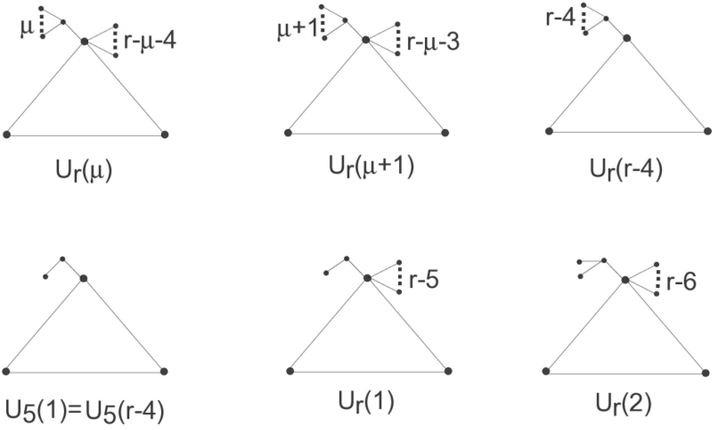
Lemma 5.

Ref. [19] If $SK(U_r(\mu ))$ is the maximum for fixed $r\ge 5$, where $1\le \mu \le r-4$, then we have $\mu =1$ or $r-4$.

Proof. 

For $r=5$, $\mu =1=r-4$ and there is only one graph $U_5(1)$. So, there cannot be a debate in choosing the maximum or minimum. Suppose that $3\le \mu \le r-5$

$$\begin{array}{ll}SK(U_r(\mu ))& =\frac{1}{2}\{2(2+r-\mu -4+3)+(r-\mu -4)(1+r-\mu -4+3)+(r-\mu -4\\ & +3+\mu +1)+\mu (1+\mu +1)+(2+2)\}=\frac{1}{2}(r^2+2{\mu }^2-r+4\mu -2r\mu +6)\end{array}$$

$$\begin{array}{l}SK(U_r(\mu +1))=\frac{1}{2}(r^2+2{\mu }^2+r+4\mu -2r\mu +10)\end{array}$$

By using the above calculations, we determine

$$SK(U_r(\mu +1))-SK(U_r(\mu ))=r+2>0$$

$$\Rightarrow SK(U_r(\mu +1))>SK(U_r(\mu ))$$

concluding that $SK(U_r(r-4))>SK(U_r(\mu ))$

• where

$$SK(U_r(r-4))=\frac{1}{2}(r^2-5r+22)$$

For $\mu =\mathrm{1,2}$, we have

$$\begin{array}{l}SK(U_r(1))=\frac{1}{2}(r^2-3r+12)\end{array}$$

$$\begin{array}{l}SK(U_r(2))=\frac{1}{2}(r^2-5r+22)\end{array}$$

Furthermore

$$SK(U_r(1))-SK(U_r(2))=r-5>0$$

$$SK(U_r(1))-SK(U_r(r-4))=r-5>0$$

$$SK(U_r(2))-SK(U_r(r-4))=0$$

By the above inequalities, we have

$$SK(U_r(1))>SK(U_r(2))=SK(U_r(r-4))>SK(U_r(\mu )),U_r(\mu );3\le \mu \le r-5$$

The above used graphs are shown in Figure 8.

So, $U_r(1)$ is the graph with the first maximum and $U_r(2)$ and $U_r(r-4)$ with the second maximum $SK$ index, and we are complete. □

Theorem 2.

Let $A$ having girth $g$ with $4\le g\le r$, be a connected unicyclic graph. Then

$$SK(A)\le SK(X_{r,g})$$

where $X_{r,g}=X(r,g;r-g,0,\dots ,0)$.

Proof. 

Let $A\in O_{r,g}$, where $O_{r,g}$ be the set of unlabeled connected unicyclic graphs having order $r$ and girth $g$ with $r\ge g>3$. If $g=r$, then $A=C_g$; for $g=r-1$ then $A=X(r,r-1;\mathrm{1,0},\dots ,0)$. Suppose that $3\le g\le r-2$ and $A$ has the largest $SK$ index. $A$ is a graph with some vertex disjoint trees having each a common vertex with $C_g$. After applying $M_1$-transformation, the trees are reduced to some stars with centers on $C_g$ and the $SK$ index strictly increases by Lemma 1. Since $SK(A)$ is the maximum, it implies that $A=X(r,g;r_1,\dots ,r_g)$ where $r_1,\dots ,r_g\ge 0$ and $r_1+\dots +r_g=r-g$. All the pendant edges attached at the vertices of $C_g$ are made incident to the unique and same vertex. After applying $M_2,M_3$-transformations several times, that would give $A=X_{r,g}=X(r,g;r-g,0,\dots ,0)$. □

Remark 1.

If $r-1\ge g\ge 3$ then $SK\left(X\left(r,g;r-g,0,\dots ,0\right)\right)>SK\left(X\left(r,g+1;r-g-\mathrm{1,0},\dots ,0\right)\right)$ by Case 1 of Lemma 1.

Lemma 6.

For $p=r-g\ge 2$, we have

(a)

$SK(A_2)<SK(A_1)$

(b)

$SK(A_3)=SK(A_1)$

(c)

$SK(A_4)<SK(A_1)$

(d)

$SK(A_5)<SK(A_1)$

(See Figure 8.)

Proof. 

$$\begin{array}{ll}& \left(a\right)SK(A_2)-SK(A_1)\\ & =\frac{1}{2}\{(2+\mu -2+2)+(\mu -2)(1+\mu -2+2)+(\mu -2+2+2)+(2+4)+(4+2)\\ & +(4+2)\}-\frac{1}{2}\{(2+\mu -1+2)+(\mu -1)(1+\mu -1+2)+(\mu -1+2+3)+(3+1)\\ & +(3+2)+(2+2)\}=-\mu +1<0.\end{array}$$

$$\begin{array}{ll}& \left(b\right)SK(A_3)-SK(A_1)\\ & =\frac{1}{2}\{(\mu -1)(1+\mu -1+2)+(\mu -1+2+2)+(2+3)+(3+1)+(3+2)\}\\ & -\frac{1}{2}\{(\mu -1)(1+\mu -1+2)+(\mu -1+2+3)+(3+1)+(3+2)+(2+2)\}=0.\end{array}$$

$$\begin{array}{ll}& \left(c\right)SK(A_4)-SK(A_1)\\ & =\frac{1}{2}\{(2+\mu -1+2)+(\mu -2)(1+\mu -2+3)+(\mu -2+3+2)+(2+1)+(\mu -1+2+2)\\ & +(2+2)\}-\frac{1}{2}\{(2+\mu -1+2)+(\mu -1)(1+\mu -1+2)+(\mu -1+2+3)+(3+1)\\ & +(3+2)\}=-1<0.\end{array}$$

$$\begin{array}{ll}& \left(d\right)SK(A_5)-SK(A_1)\\ & =\frac{1}{2}\{(2+3)+(3+\mu -1+1)+(\mu -1)(1+\mu -1+1)+(3+2)+(2+2)\}\\ & -\frac{1}{2}\{(2+\mu -1+2)+(\mu -1)(1+\mu -1+2)+(\mu -1+2+3)+(3+1)+(3+2)\}=-\mu +1<0.\end{array}\square$$

Theorem 3.

(a) Let $A\in O_{r,g}\backslash \{X_{r,g}\}$, where $r\ge 6,(4\le g\le r-2)$. Then $A$ has a maximum $SK$ index if, and only if, $A=A_1(=A_3)$.

(b) Let $A\in O_{r,g}\backslash \{(A_1\cup X_{r,g})\}$, where $r\ge 6,(4\le g\le r-2)$. Then $A$ has a maximum $SK$ index if, and only if, $A=X(r,g;r-g-\mathrm{2,0},\mathrm{2,0},\dots ,0)=A_2$.

Proof. 

Let $A\in O_{r,g}$ be a connected unicyclic graph having the second or third maximum $SK$ index. Suppose that there is a vertex with a degree of at least 3 in a cycle $C_g$ of $A$. Since $A\ne X_{r,g}$, then there is at least one non-pendant vertex in $C$.

Case 1: When there is exactly one non-pendant vertex outside $C$, we obtained $A$ by attaching the $\mu$ pendant edges to a pendant vertex of $X(r-\mu ,g;r-g-\mu ,0,\dots ,0)$ where $(1\le \mu \le r-g-1)$. Lemma 5 states that for $\mu =1$ or $r-4$ we have a maximum of $SK(U_r(\mu ))$ with corresponding graphs $A_4$ and $A_5$, respectively.

However, Lemma 6 implies that the graphs with the second or third maximum $SK$ index cannot be $A_4$ or $A_5$.

Case 2: When there are at least two non-pendant vertices outside $C,$ after the continuous application of $M_1$-transformation, we have

$$SK(A)<max\{SK(A_4),SK(A_5)\}<SK(A_3)=SK(A_1)<SK(X_{r,g})$$

$$\mathrm{as}SK(A_1)-SK(X_{r,g})=\{\frac{1}{2}(r^2+g^2+3r+g-2rg+2)\}-\{\frac{1}{2}(r^2+g^2+5r-g-2rg)\}=-r+g+1<0$$

(7)

Thus, we knew that if $A$ has a second or third maximum $SK$ index then the two vertices on $C_g$ must exist having a degree of at least three.

(a) For $A\ne X_{r,g}$, if $A$ has a maximum $SK$ then $C_g$ cannot have three vertices with a degree of at least 3.

We obtained $X_{r,g}$ after several applications of $M_i$-transformations $(i\ge 1)$. However, we found a graph with an index less than $X_{r,g}$, we see that

$$SK(A)<max\{SK(A_3),SK(A_1)\}=SK(A_3)=SK(A_1)<SK(X_{r,g})$$

It implies that $A$ has exactly two vertices $m,n$ on $C_g$ having a degree of at least 3.

Degrees of $m$ and $n$ must be as: $d(m)=r-g+1,d(n)=3$, since other cases cannot hold because if $d(m)=2$ then $A$ becomes $X_{r,g}$ (since our supposition of the degree is at least $3$) and if $d(m)=4$ then $A$ cannot become the second maximum because $A$ with $d(m)=3$ has a greater index than $A$ with $d(m)=4$.

Now, if $d(m,n)=1$ then $A=A_1$ and if $d(m,n)\ge 2$ then $A\in Y(r,g)$ class including $A_3$.

Lemma 6 implies that, in this case, extremal graph is $A_1$.

(b) For $A\in O_{r,g}\backslash (A_1\cup X_{r,g})$, by the same argument we deduce that $C_g$ cannot have three vertices with a degree of at least 3, if $A$ has a maximum $SK$ index, since, in this case, we would have

$$SK(A)<SK(A_2)<SK(A_3)=SK(A_1)<SK(X_{r,g})$$

$$\mathrm{as}SK\left(A_2\right)-SK\left(A_1\right)=\left\{\frac{1}{2}\left(r^2+g^2+r+3g-2rg+4\right)\right\}-\left\{\frac{1}{2}\left(r^2+g^2+3r+g-2rg+2\right)\right\}$$

$$=\frac{1}{2}(-2r+2g+2)=-r+g+1<0$$

It implies that $A$ has exactly two vertices $a,b$ on $C_g$ having a degree of at least 3.

By the same argument (used above), $d(m)=r-g$ and $d(n)=4$.

If $d(m,n)=1$ then $A=A_6$ and if $d(m,n)\ge 2$ then $A\in Z(r,g)$ class including $A_2$, which ends the proof(see Figure 9). □

3. Ordering Unicyclic Structures with the Greatest SK₁ Index

In this section, we use graph transformations which increase the $S{K}_1$ index.

Lemma 7.

Let $M_1(A)$ be a unicyclic connected graph as shown in Figure 1, then

$$S{K}_1(A)<S{K}_1(M_1(A))$$

for any $\mu ,v\ge 0$.

Proof. 

Case 1: Ref. [19] When $M_1$ is performed excluding vertices of $C_g$

$$\begin{array}{ll}S{K}_1(A)-S{K}_1(M_1(A))& =\frac{1}{2}{\displaystyle \sum _{xy\in E(A)\backslash \{yz\}}}[(d_x.d_y)-(d_x)(d_y+d_z-1)]\\ & +\frac{1}{2}{\displaystyle \sum _{xz\in E(A)\backslash \{yz\}}}[(d_x.d_z)-(d_x)(d_y+d_z-1)]<0;as{d}_y\ge 2\end{array}$$

Case 2: When $M_1$ is performed on vertices of $C_g$

We have $d_A({\omega }_i)=d_{M_1(A)}({\omega }_i)-v-1<d_{M_1(A)}({\omega }_i)$ and $d_{M_1(A)}({\omega }_i)+d_{M_1(A)}({\omega }_{i+1})=\mu +v+4$.

Therefore, for $j=\overline{1,\mu }=\mathrm{1,2},\dots ,\mu$, $k=\overline{1,v}=\mathrm{1,2},\dots ,v$ and by the definition of the $S{K}_1$ index, we find

$$\begin{array}{ll}S{K}_1(A)-S{K}_1(M_1(A))& =\frac{1}{2}[\{d({\omega }_{i-1}).d({\omega }_i)\}+\mu \{d({\omega }_{i,j}).d({\omega }_i)\}+\{d({\omega }_i).d({\omega }_{i+1})\}\\ & +\nu \{d({\omega }_{i+1,k}).d({\omega }_{i+1})\}+\{d({\omega }_{i+1}).d({\omega }_{i+2})\}]-\frac{1}{2}[\{d({\omega }_{i-1}).d({\omega }_i)\}\\ & +(\mu +\nu +1)\{d({\omega }_{i,j}).d({\omega }_i)\}+\{d({\omega }_i).d({\omega }_{i+2})\}]\\ & =\frac{1}{2}[\{(2)(\mu +2)\}+\mu \{(1)(\mu +2)\}\{(\mu +2)(\nu +2)\}\\ & +\nu \{(1)(\nu +2)\}+\{(\nu +2)(2)\}]-\frac{1}{2}[\{(2)(\mu +\nu +3)\}\\ & +(\mu +\nu +1)\{(1)(\mu +\nu +3)\}+\{(\mu +\nu +3)(2)\}]\\ & =-\{\mu +\nu +\frac{1}{2}(3+\mu \nu )\}<0for\mu ,\nu \ge 1.\end{array}$$

$$\Rightarrow S{K}_1(A)<S{K}_1(M_1(A))\square$$

Lemma 8.

Let $M_2(A)$ be a unicyclic connected graph as depicted in Figure 2, where $d_A({\omega }_i,{\omega }_{i+1})=1$. Then

$$S{K}_1(A)<S{K}_1(M_2(A))$$

for any $v\ge \mu \ge 1$.

Proof. 

Since $d_{M_2(A)}({\omega }_i)=2<d_A({\omega }_i)=\mu +2$ and $d_A({\omega }_{i+1})=\nu +2<d_{M_2(A)}({\omega }_{i+1})=\nu +\mu +2$.

$$\begin{array}{ll}S{K}_1(A)-S{K}_1(M_2(A))& =\frac{1}{2}[\{d({\omega }_{i-1}).d({\omega }_i)\}+{\displaystyle \sum _{j=1}^{\mu }}\{d({\omega }_{i,j}).d({\omega }_i)\}+\{d({\omega }_i).d({\omega }_{i+1})\}\\ & +{\displaystyle \sum _{k=1}^{\nu }}\{d({\omega }_{i+1,k}).d({\omega }_{i+1})\}+\{d({\omega }_{i+1}).d({\omega }_{i+2})\}]\\ & \frac{1}{2}[\{d({\omega }_{i-1}).d({\omega }_i)\}+\{d({\omega }_i).d({\omega }_{i+1})\}+(\mu +\nu )\{d({\omega }_{i,j}).d({\omega }_{i+1})\}\\ & +\{d({\omega }_{i+1}).d({\omega }_{i+2})\}]\\ & =\frac{1}{2}[\{d({\omega }_{i-1}).d({\omega }_i)\}+\mu \{d({\omega }_{i,j}).d({\omega }_i)\}+\{d({\omega }_i).d({\omega }_{i+1})\}\\ & +\nu \{d({\omega }_{i+1,k}).d({\omega }_{i+1})\}+\{d({\omega }_{i+1}).d({\omega }_{i+2})\}]\\ & \frac{1}{2}[\{d({\omega }_{i-1}).d({\omega }_i)\}+\{d({\omega }_i).d({\omega }_{i+1})\}+(\mu +\nu )\{d({\omega }_{i,j}).d({\omega }_{i+1})\}\\ & +\{d({\omega }_{i+1}).d({\omega }_{i+2})\}]\\ & =\frac{1}{2}\{(2)(\mu +2)+\mu (1)(\mu +2)+(\mu +2)(\nu +2)+\nu (1)(\nu +2)\\ & +(\nu +2)(2)\}-\frac{1}{2}\{(2)(2)+(2)(\mu +\nu +2)+(\mu +\nu )(1)(\mu +\nu +2)\\ & +(\mu +\nu +2)(2)\}\\ & =-\frac{1}{2}(\mu \nu )<0for\nu \ge \mu \ge 1.\end{array}$$

$$\Rightarrow S{K}_1(A)<S{K}_1(M_2(A))\square$$

Lemma 9.

Let  $M_3(A)$ be a unicyclic connected graph as presented in Figure 3, where $d_A({\omega }_i,{\omega }_{i+1})=d_{M_3(A)}({\omega }_i,{\omega }_{i+1})\ge 2$. Then

$$S{K}_1(A)<S{K}_1(M_3(A));v\ge \mu \ge 1$$

Proof. 

Following the previous lemma and by the definition of $S{K}_1(A)$, we find

$$\begin{array}{ll}S{K}_1(A)-S{K}_1(M_3(A))& =\frac{1}{2}[\{d({\omega }_{i-1}).d({\omega }_i)\}+{\displaystyle \sum _{k=1}^{\mu }}\{d({\omega }_{i,j}).d({\omega }_i)\}+\{d({\omega }_i).d({\omega }_{i+1})\}\\ & +\{d({\omega }_{i+1}).d({\omega }_j)\}+{\displaystyle \sum _{l=1}^{\nu }}\{d({\omega }_{j,\nu }).d({\omega }_j)\}+\{d({\omega }_j).d({\omega }_{j+1})\}]\\ & -\frac{1}{2}[\{d({\omega }_{i-1}).d({\omega }_i)\}+{\displaystyle \sum _{k=1}^{\mu -1}}\{d({\omega }_{i,\mu -1}).d({\omega }_i)\}+\{d({\omega }_i).d({\omega }_{i+1})\}\\ & +\{d({\omega }_{i+1}).d({\omega }_j)\}+{\displaystyle \sum _{l=1}^{\nu +1}}\{d({\omega }_{j,\nu }).d({\omega }_j)\}+\{d({\omega }_j).d({\omega }_{j+1})\}]\\ & =\frac{1}{2}[\{d({\omega }_{i-1}).d({\omega }_i)\}+\mu \{d({\omega }_{i,j}).d({\omega }_i)\}+\{d({\omega }_i).d({\omega }_{i+1})\}\\ & +\{d({\omega }_{i+1}).d({\omega }_j)\}+\nu \{d({\omega }_{j,\nu }).d({\omega }_j)\}+\{d({\omega }_j).d({\omega }_{j+1})\}]\\ & -\frac{1}{2}[\{d({\omega }_{i-1}).d({\omega }_i)\}+(\mu -1)\{d({\omega }_{i,\mu -1}).d({\omega }_i)\}+\{d({\omega }_i).d({\omega }_{i+1})\}\\ & +\{d({\omega }_{i+1}).d({\omega }_j)\}+(\nu +1)\{d({\omega }_{j,\nu }).d({\omega }_j)\}+\{d({\omega }_j).d({\omega }_{j+1})\}]\\ & =\frac{1}{2}\{(2)(\mu +2)+\mu (1)(\mu +2)+(\mu +2)(2)+(2)(\nu +2)\\ & +\nu (1)(\nu +2)+(\nu +2)(2)\}-\frac{1}{2}\{2(\mu -1+2)+(\mu -1)(1)\\ & (\mu -1+2)+(\mu -1+2)(2)+(2)(1+\nu +2)+(\nu +1)(1)(\nu +1+2)\\ & +(\nu +1+2)(2)\}\\ & =\frac{1}{2}(2\mu -2\nu -2)=\mu -\nu -1<0\nu \ge \mu \ge 1\end{array}$$

$$\Rightarrow S{K}_1(A)<S{K}_1(M_3(A))\square$$

Hence, the proof is complete.

Lemma 10.

Let $M_4(A)$ be the graph attained from $A$ as illustrated in Figure 4. For any $\nu \ge \mu \ge 1$, we have

$$S{K}_1(A)<S{K}_1(M_4(A))$$

Proof. 

If $d_A({\omega }_i,{\omega }_{i+1})=1$ then $d_{M_4(A)}({\omega }_i)+d_{M_4(A)}({\omega }_{i+1})=\mu +2+v+2=d_A({\omega }_i)+d_A({\omega }_j)$ and by the definition of $S{K}_1(A)$, we have

$$\begin{array}{ll}S{K}_1(A)-S{K}_1(M_4(A))& =\frac{1}{2}[\{d({\omega }_{i-1}).d({\omega }_i)\}+{\displaystyle \sum _{j=1}^{\mu }}\{d({\omega }_{i,j}).d({\omega }_i)\}+\{d({\omega }_i).d({\omega }_{i+1})\}\\ & +{\displaystyle \sum _{k=1}^{\nu }}\{d({\omega }_{i+1,k}).d({\omega }_{i+1})\}+\{d({\omega }_{i+1}).d({\omega }_{i+2})\}]-\frac{1}{2}[\{d({\omega }_{i-1})\\ & .d({\omega }_i)\}+{\displaystyle \sum _{j=1}^{\mu -1}}\{d({\omega }_{i,\mu -1}).d({\omega }_i)\}+\{d({\omega }_i).d({\omega }_{i+1})\}\\ & +{\displaystyle \sum _{k=1}^{\nu +1}}\{d({\omega }_{i+1,k}).d({\omega }_{i+1})\}+\{d({\omega }_{i+1}).d({\omega }_{i+2})\}]\\ & =\frac{1}{2}[\{d({\omega }_{i-1}).d({\omega }_i)\}+\mu \{d({\omega }_{i,j}).d({\omega }_i)\}+\{d({\omega }_i).d({\omega }_{i+1})\}\\ & +\nu \{d({\omega }_{i+1,k}).d({\omega }_{i+1})\}+\{d({\omega }_{i+1}).d({\omega }_{i+2})\}]-\frac{1}{2}[\{d({\omega }_{i-1})\\ & .d({\omega }_i)\}+(\mu -1)\{d({\omega }_{i,\mu -1}).d({\omega }_i)\}+\{d({\omega }_i).d({\omega }_{i+1})\}\\ & +(\nu +1)\{d({\omega }_{i+1,k}).d({\omega }_{i+1})\}+\{d({\omega }_{i+1}).d({\omega }_{i+2})\}]\\ & =\frac{1}{2}\{(2)(\mu +2)+\mu (1)(\mu +2)+(\mu +2)(\nu +2)+\nu (1)(\nu +2)\\ & +(\nu +2)(2)\}-\frac{1}{2}\{(2)(\mu -1+2)+(\mu -1)(1)(\mu -1+2)\\ & +(\mu -1+2)(\nu +1+2)+(\nu +1)(1)(\nu +1+2)+(\nu +1+2)(2)\}\\ & =\frac{1}{2}(\mu -\nu -1)<0for\nu \ge \mu \ge 1.\end{array}$$

$$\Rightarrow S{K}_1(A)<S{K}_1(M_4(A))\square$$

Now first, we find the extremal graphs having the greatest value and then give an ordering of the unicyclic connected graphs in decreasing order for the $S{K}_1$ index.

Theorem 4

Ref. [19]. Let $X(r,3;a,b,c)$; $a+b+c=r-3$; $a\ge b\ge c\ge 1$ be a set of unicyclic connected graphs with $r\ge 5$. Then the first maximum and second maximum values of the $S{K}_1$ index are attained by $X(r,3;r-\mathrm{3,0},0)$ and $X(r,3;r-\mathrm{4,1},0)$, respectively, i.e.,

$$S{K}_1(X(r,3;r-\mathrm{4,1},0))<S{K}_1(X(r,3;r-\mathrm{3,0},0))$$

(See Figure 7.)

Proof. 

We need only to prove $S{K}_1(X(r,3;a,b,c))<S{K}_1(X(r,3;a+1,b-1,c))$.

Consider

$$\begin{array}{ll}& S{K}_1(X(r,3;a,b,c))-S{K}_1(X(r,3;a+1,b-1,c))\\ & =\frac{1}{2}\{a(1)(a+2)+(a+2)(b+2)+b(1)(b+2)+(b+2)(c+2)+c(1)(c+2)\\ & +(c+2)(a+2)\}-\frac{1}{2}\{(a+1)(1)(a+1+2)+(a+1+2)(b-1+2)\\ & +(b-1)(1)(b-1+2)+(b-1+2)(c+2)+c(1)(c+2)+(c+2)(a+1+2)\}\\ & =\frac{1}{2}(-a+b-1)<0fora\ge b\ge c\ge 1.\end{array}\square$$

Hence, the result follows.

Lemma 11.

Ref. [19] If $S{K}_1(U_r(\mu ))$ is the maximum for fixed $r\ge 5$, where $1\le \mu \le r-4$, then we have $\mu =1$ or $r-4$.

Proof. 

For $r=5$, $\mu =1=r-4$ and there is only one graph $U_5(1)$. So, there cannot be a debate in choosing the maximum or the minimum.

Suppose that $3\le \mu \le r-5$

$$\begin{array}{ll}S{K}_1(U_r(\mu ))& =\frac{1}{2}\{2(2)(r-\mu -4+3)+(r-\mu -4)(1)(r-\mu -4+3)+(r-\mu -4+3)\\ & (\mu +1)+\mu (1)(\mu +1)+(2)(2)\}=\frac{1}{2}(r^2+{\mu }^2-r\mu +3)\end{array}$$

$$\begin{array}{l}S{K}_1(U_r(\mu +1))=\frac{1}{2}(r^2+{\mu }^2+3r-r\mu +6)\end{array}$$

By using the above calculations, we determine

$$S{K}_1(U_r(\mu +1))-S{K}_1(U_r(\mu ))=\frac{3}{2}(r+1)>0$$

$$\Rightarrow S{K}_1(U_r(\mu +1))>S{K}_1(U_r(\mu ))$$

concluding that $S{K}_1(U_r(\mu ))>S{K}_1(U_r(r-4))$

• where

$$S{K}_1(U_r(r-4))=\frac{1}{2}(r^2-4r+19)$$

For $p=\mathrm{1,2}$, we have

$$\begin{array}{l}S{K}_1(U_r(1))=\frac{1}{2}(r^2-r+4)\end{array}$$

$$\begin{array}{l}S{K}_1(U_r(2))=\frac{1}{2}(r^2-2r+7)\end{array}$$

Furthermore

$$S{K}_1(U_r(1))-S{K}_1(U_r(2))=\frac{1}{2}(r-3)>0$$

$$S{K}_1(U_r(1))-S{K}_1(U_r(r-4))=\frac{3}{2}(r-5)>0$$

$$S{K}_1(U_r(2))-S{K}_1(U_r(r-4))=r-6>0$$

By the above inequalities, we have

$$S{K}_1\left(U_r\left(1\right)\right)>S{K}_1\left(U_r\left(2\right)\right)>S{K}_1\left(U_r\left(\mu \right)\right)>S{K}_1\left(U_r\left(r-4\right)\right),U_r\left(\mu \right);3\le \mu \le r-5$$

The above used graphs are shown in Figure 8. Therefore, $U_r(1)$ is a graph with the first maximum and $U_r(2)$ with the second maximum $S{K}_1$ index, and we are complete. □

Theorem 5.

Let $A$ having girth $g$ with $4\le g\le r$, be a connected unicyclic graph. Then

$$S{K}_1(A)\le S{K}_1(X_{r,g})$$

where $X_{r,g}=X(r,g;r-g,0,\dots ,0)$.

Proof. 

Let $A\in O_{r,g}$, where $O_{r,g}$ be the set of unlabelled connected unicyclic graphs having order $r$ and girth $g$ with $r\ge g>3$. If $g=r$, then $A=C_g$; for $g=r-1$ then $A=X(r,r-1;\mathrm{1,0},\dots ,0)$. Suppose that $3\le g\le r-2$ and $A$ has the largest $S{K}_1$ index. $A$ is a graph with some vertex disjoint trees having each a common vertex with $C_g$. After applying $M_1$-transformation, the trees are reduced to some stars with centers on $C_g$ and the $S{K}_1$ index strictly increases by Lemma 7. Since $S{K}_1(A)$ is the maximum, it implies that $A=X(r,g;r_1,\dots ,r_g)$ where $r_1,\dots ,r_g\ge 0$ and $r_1+\dots +r_g=r-g$. All the pendant edges attached at the vertices of $C_g$ are made incident to the unique and same vertex. After applying $M_2,M_3$-transformations several times, that would give $A=X_{r,g}=X(r,g;r-g,0,\dots ,0)$. □

Remark 2.

If $r-1\ge g\ge 3$ then $S{K}_1(X(r,g;r-g,0,\dots ,0))>S{K}_1(X(r,g+1;r-g-\mathrm{1,0},\dots ,0))$ by Case 1 of Lemma 7.

Lemma 12.

(1) For $p=r-g\ge 3$, we have

$$S{K}_1(A_2)<S{K}_1(A_1)$$

(2) For $p=r-g\ge 2$, we have

(a)

$S{K}_1(A_3)<S{K}_1(A_1)$.

(b)

$S{K}_1(A_4)<S{K}_1(A_1)$.

(c)

$S{K}_1(A_5)<S{K}_1(A_1)$.

See Figure 6.

Proof. 

$$\begin{array}{ll}& S{K}_1(A_2)-S{K}_1(A_1)\\ & =\frac{1}{2}\{(2)(\mu -2+2)+(\mu -2)(1)(\mu -2+2)+(\mu -2+2)(2)+(2)(4)+(4)(2)+(4)(2)\}\\ & -\frac{1}{2}\{(2)(\mu -1+2)+(\mu -1)(1)(\mu -1+2)+(\mu -1+2)(3)+(3)(1)+(3)(2)+(2)(2)\}\\ & =\frac{1}{2}(-3\mu +7)<0.\end{array}$$

$$\begin{array}{ll}& \left(a\right)S{K}_1(A_3)-S{K}_1(A_1)\\ & =\frac{1}{2}\{(\mu -1)(1)(\mu -1+2)+(\mu -1+2)(2)+(2)(3)+(3)(1)+(3)(2)\}\\ & -\frac{1}{2}\{(\mu -1)(1)(\mu -1+2)+(\mu -1+2)(3)+(3)(1)+(3)(2)+(2)(2)\}\\ & =\frac{1}{2}(-\mu +1)<0.\end{array}$$

$$\begin{array}{ll}& \left(b\right)S{K}_1(A_4)-S{K}_1(A_1)\\ & =\frac{1}{2}\{(2+\mu -1)(2)+(\mu -2)(1)(\mu -2+3)+(\mu -2+3)(2)+(2)(1)+(\mu -1+2)(2)\\ & +(2)(2)\}-\frac{1}{2}\{(2+\mu -1)(2)+(\mu -1)(1)(\mu -1+2)+(\mu -1+2)(3)+(3)(1)+(3)(2)\}\\ & =-\frac{3}{2}<0.\end{array}$$

$$\begin{array}{ll}& \left(c\right)S{K}_1(A_5)-S{K}_1(A_1)\\ & =\frac{1}{2}\{(2)(3)+(3)(\mu -1+1)+(\mu -1)(1)(\mu -1+1)+(3)(2)+(2)(2)\}\\ & -\frac{1}{2}\{(2)(\mu -1+2)+(\mu -1)(1)(\mu -1+2)+(\mu -1+2)(3)+(3)(1)+(3)(2)\}\\ & =\frac{1}{2}(-3\mu +3)<0.\end{array}\square$$

Theorem 6.

(a) Let $A\in O_{r,g}\backslash \{X_{r,g}\}$, where $r\ge 6,(4\le g\le r-2)$. Then $A$ has a maximum $S{K}_1$ index if, and only if, $A=A_1$.

(b) Let $A\in O_{r,g}\backslash \{(A_1\cup X_{r,g})\}$, where $r\ge 7,(4\le g\le r-3)$. Then $A$ has a maximum $S{K}_1$ index if, and only if, $A=X(r,g;r-g-\mathrm{1,0},\mathrm{1,0},\dots ,0)=A_3$.

Proof. 

Let $A\in O_{r,g}$ be a connected unicyclic graph having the second or third maximum $S{K}_1$ index. Suppose that there is a vertex with a degree of at least 3 in a cycle $C_g$ of $A$. Since $A\ne X_{r,g}$, then there is at least one non-pendant vertex in $C$.

Case 1: When there is exactly one non-pendant vertex outside $C,$ we obtained $A$ by attaching the $\mu$ pendant edges to a pendant vertex of $X(r-\mu ,g;r-g-\mu ,0,\dots ,0)$ where $(1\le \mu \le r-g-1)$.

Lemma 11 states that for $\mu =1$ or $r-4$ we have the maximum of $S{K}_1(U_r(\mu ))$ with corresponding graphs $A_4$ and $A_5$.

However, Lemma 12 implies that the graphs with the second or third maximum $S{K}_1$ index, cannot be $A_4$ or $A_5$.

Case 2: When there are at least two non-pendant vertices outside $C$, after the continuous application of $M_1$-transformation, we have

$$S{K}_1(A)<max\{S{K}_1(A_4),S{K}_1(A_5)\}<S{K}_1(A_3)<S{K}_1(A_1)<S{K}_1(X_{r,g})$$

$$\begin{array}{c}\mathrm{as}S{K}_1(A_1)-S{K}_1(X_{r,g})=\{\frac{1}{2}(r^2+g^2+5r-g-2rg+1)\}-\{\frac{1}{2}(r^2+g^2+\\ 6r-2g-2rg)\}=\frac{1}{2}(-r+g+1)<0\end{array}$$

Thus, we knew that if $A$ has a second or third maximum $S{K}_1$ index then the two vertices on $C_g$ must exist having a degree of at least three.

(a) For $A\ne X_{r,g}$, if $A$ has a maximum $S{K}_1$ then $C_g$ cannot have three vertices with a degree of at least 3.

We obtained $X_{r,g}$ after several applications of $M_i$-transformations $(i\ge 1)$. However, we found a graph with an index less than $X_{r,g}$, we see that

$$S{K}_1(A)<max\{S{K}_1(A_3),S{K}_1(A_1)\}=S{K}_1(A_1)<S{K}_1(X_{r,g})$$

It implies that $A$ has exactly two vertices $m,n$ on $C_g$ having a degree of at least 3.

Degrees of $m$ and $n$ must be as: $d(m)=r-g+1,d(n)=3$, since other cases cannot hold because if $d(m)=2$ then $A$ becomes $X_{r,g}$ (since our supposition of degree is at least $3$) and if $d(m)=4$ then $A$ cannot become the second maximum because $A$ with $d(m)=3$ has a greater index than $A$ with $d(m)=4$.

Now, if $d(m,n)=1$ then $A=A_1$ and if $d(m,n)\ge 2$ then $A\in Y(r,g)$ class including $A_3$.

Lemma 12 implies that, in this case, the extremal graph is $A_1$.

(b) For $A\in O_{r,g}\backslash (A_1\cup X_{r,g})$, by the same argument we deduce that $C_g$ cannot have three vertices with a degree of at least 3, if $A$ has a maximum ${SK}_1$ index, since, in this case, we would have

$$S{K}_1(A)<S{K}_1(A_3)<S{K}_1(A_1)<S{K}_1(X_{r,g})$$

$$\begin{array}{c}\mathrm{as}S{K}_1(A_3)-S{K}_1(A_1)=\{\frac{1}{2}(r^2+g^2+4r-2rg+2)\}-\{\frac{1}{2}(r^2+g^2+5r-\\ g-2rg+1)\}=\frac{1}{2}(-r+g+2)<0\end{array}$$

It implies that $A$ has exactly two vertices $a,b$ on $C_g$ having a degree of at least 3. By the same argument (used above), $d(m)=r-g$ and $d(n)=4$.

If $d(m,n)=1$ then $A=A_6$ and if $d(m,n)\ge 2$ then $A\in Z(r,g)$ class including $A_2$, which ends the proof. □

(See Figure 10.)

4. Ordering Unicyclic Structures with the Greatest SK₂ Index

In this section, we use graph transformations which increase the $S{K}_2$ index.

Lemma 13.

Let $M_1(A)$ be a unicyclic connected graph as shown in Figure 1, then

$$S{K}_2(A)<S{K}_2(M_1(A))$$

for any $\mu ,v\ge 0$.

Proof. 

Case 1: Ref. [19] When $M_1$ is performed excluding the vertices of $C_g$

$$\begin{array}{ll}S{K}_2(A)-S{K}_2(M_1(A))& =\frac{1}{4}{\displaystyle \sum _{xy\in E(A)\backslash \{yz\}}}[(d_x+d_y{)}^2-(d_x+d_y+d_z-1{)}^2]\\ & +\frac{1}{4}{\displaystyle \sum _{xz\in E(A)\backslash \{yz\}}}[(d_x+d_z{)}^2-(d_x+d_y+d_z-1{)}^2]<0;as{d}_y\ge 2\end{array}$$

Case 2: When $M_1$ is performed on the vertices of $C_g$

We have $d_A({\omega }_i)=d_{M_1(A)}({\omega }_i)-v-1<d_{M_1(A)}({\omega }_i)$ and $d_{M_1(A)}({\omega }_i)+d_{M_1(A)}({\omega }_{i+1})=\mu +v+4$.

Therefore, for $j=\overline{1,\mu }=\mathrm{1,2},\dots ,\mu$, $k=\overline{1,v}=\mathrm{1,2},\dots ,v$ and by the definition of the $S{K}_2$ index, we find

$$\begin{array}{ll}S{K}_2(A)-S{K}_2(M_1(A))& =\frac{1}{4}[\{d({\omega }_{i-1})+d({\omega }_i){\}}^2+\mu \{d({\omega }_{i,j})+d({\omega }_i){\}}^2+\{d({\omega }_i)\\ & +d({\omega }_{i+1}){\}}^2+\nu \{d({\omega }_{i+1,k})+d({\omega }_{i+1}){\}}^2+\{d({\omega }_{i+1})+d({\omega }_{i+2}){\}}^2]\\ & -\frac{1}{4}[\{d({\omega }_{i-1})+d({\omega }_i){\}}^2+(\mu +\nu +1)\{d({\omega }_{i,j})+d({\omega }_i){\}}^2\\ & +\{d({\omega }_i)+d({\omega }_{i+2}){\}}^2]\\ & =\frac{1}{4}\{(2+\mu +2{)}^2+\mu (1+\mu +2{)}^2+(\mu +2+\nu +2{)}^2+\nu (1+\nu +2{)}^2\\ & +(\nu +2+2{)}^2\}-\frac{1}{4}\{(2+\mu +\nu +1+2{)}^2+(\mu +\nu +1)\\ & (1+\mu +\nu +1+2{)}^2+(\mu +\nu +1+2+2{)}^2\}\\ & =-\frac{1}{4}(3{\mu }^2+3{\nu }^2+19\mu +19\nu +20\mu \nu +3{\mu }^2\nu +3\mu {\nu }^2+18)<0.\end{array}$$

$$\Rightarrow S{K}_2(A)<S{K}_2(M_1(A))\square$$

Lemma 14.

Let $M_2(A)$ be a unicyclic connected graph as depicted in Figure 2, where $d_A({\omega }_i,{\omega }_{i+1})=1$. Then

$$S{K}_2(A)<S{K}_2(M_2(A))$$

for any $v\ge \mu \ge 1$.

Proof. 

Since $d_{M_2(A)}({\omega }_i)=2<d_A({\omega }_i)=\mu +2$ and $d_A({\omega }_{i+1})=\nu +2<d_{M_2(A)}({\omega }_{i+1})=\nu +\mu +2$.

$$\begin{array}{ll}S{K}_2(A)-S{K}_2(M_2(A))& =\frac{1}{4}[\{d({\omega }_{i-1})+d({\omega }_i){\}}^2+{\displaystyle \sum _{j=1}^{\mu }}\{d({\omega }_{i,j})+d({\omega }_i){\}}^2+\{d({\omega }_i)\\ & +d({\omega }_{i+1}){\}}^2+{\displaystyle \sum _{k=1}^{\nu }}\{d({\omega }_{i+1,k})+d({\omega }_{i+1}){\}}^2+\{d({\omega }_{i+1})+d({\omega }_{i+2}){\}}^2]\\ & -\frac{1}{4}[\{d({\omega }_{i-1})+d({\omega }_i){\}}^2+\{d({\omega }_i)+d({\omega }_{i+1}){\}}^2\\ & +(\mu +\nu )\{d({\omega }_{i,j})+d({\omega }_{i+1}){\}}^2+\{d({\omega }_{i+1})+d({\omega }_{i+2}){\}}^2]\\ & =\frac{1}{4}[\{d({\omega }_{i-1})+d({\omega }_i){\}}^2+\mu \{d({\omega }_{i,j})+d({\omega }_i){\}}^2+\{d({\omega }_i)\\ & +d({\omega }_{i+1}){\}}^2+\nu \{d({\omega }_{i+1,k})+d({\omega }_{i+1}){\}}^2+\{d({\omega }_{i+1})+d({\omega }_{i+2}){\}}^2]\\ & -\frac{1}{4}[\{d({\omega }_{i-1})+d({\omega }_i){\}}^2+\{d({\omega }_i)+d({\omega }_{i+1}){\}}^2\\ & +(\mu +\nu )\{d({\omega }_{i,j})+d({\omega }_{i+1}){\}}^2+\{d({\omega }_{i+1})+d({\omega }_{i+2}){\}}^2]\\ & =\frac{1}{4}\{(2+\mu +2{)}^2+\mu (1+\mu +2{)}^2+(\mu +2+\nu +2{)}^2+\nu \\ & (1+\nu +2{)}^2+(\nu +2+2{)}^2\}-\frac{1}{4}\{(2+2{)}^2+(2+\mu +\nu +2{)}^2\\ & +(\mu +\nu )(1+\mu +\nu +2{)}^2+(\mu +\nu +2+2{)}^2\}\\ & =-\frac{\mu \nu }{4}(3\mu +3\nu +14)<0for\nu \ge \mu \ge 1.\end{array}$$

$$\Rightarrow S{K}_2(A)<S{K}_2(M_2(A))\square$$

Lemma 15.

Let $M_3(A)$ be a unicyclic connected graph as presented in Figure 3, where $d_A({\omega }_i,{\omega }_{i+1})=d_{M_3(A)}({\omega }_i,{\omega }_{i+1})\ge 2$. Then

$$S{K}_2(A)<S{K}_2(M_3(A));v\ge \mu \ge 1$$

Proof. 

Following the previous lemma and by the definition of $S{K}_2(A)$, we find

$$\begin{array}{ll}S{K}_2(A)-S{K}_2(M_3(A))& =\frac{1}{4}[\{d({\omega }_{i-1})+d({\omega }_i){\}}^2+{\displaystyle \sum _{k=1}^{\mu }}\{d({\omega }_{i,j})+d({\omega }_i){\}}^2\\ & +\{d({\omega }_i)+d({\omega }_{i+1}){\}}^2+\{d({\omega }_{i+1})+d({\omega }_j){\}}^2+{\displaystyle \sum _{l=1}^{\nu }}\{d({\omega }_{j,\nu })+d({\omega }_j){\}}^2\\ & +\{d({\omega }_j)+d({\omega }_{j+1}){\}}^2]-\frac{1}{4}[\{d({\omega }_{i-1})+d({\omega }_i){\}}^2+{\displaystyle \sum _{k=1}^{\mu -1}}\\ & \{d({\omega }_{i,\mu -1})+d({\omega }_i){\}}^2+\{d({\omega }_i)+d({\omega }_{i+1}){\}}^2+\{d({\omega }_{i+1})\\ & +d({\omega }_j){\}}^2+{\displaystyle \sum _{l=1}^{\nu +1}}\{d({\omega }_{j,\nu })+d({\omega }_j){\}}^2+\{d({\omega }_j)+d({\omega }_{j+1}){\}}^2]\\ & =\frac{1}{4}[\{d({\omega }_{i-1})+d({\omega }_i){\}}^2+\mu \{d({\omega }_{i,j})+d({\omega }_i){\}}^2\\ & +\{d({\omega }_i)+d({\omega }_{i+1}){\}}^2+\{d({\omega }_{i+1})+d({\omega }_j){\}}^2+\nu \{d({\omega }_{j,\nu })+d({\omega }_j){\}}^2\\ & +\{d({\omega }_j)+d({\omega }_{j+1}){\}}^2]-\frac{1}{4}[\{d({\omega }_{i-1})+d({\omega }_i){\}}^2+(\mu -1)\\ & \{d({\omega }_{i,\mu -1})+d({\omega }_i){\}}^2+\{d({\omega }_i)+d({\omega }_{i+1}){\}}^2+\{d({\omega }_{i+1})\\ & +d({\omega }_j){\}}^2+(\nu +1)\{d({\omega }_{j,\nu })+d({\omega }_j){\}}^2+\{d({\omega }_j)+d({\omega }_{j+1}){\}}^2]\\ & =\frac{1}{4}\{(2+\mu +2{)}^2+\mu (1+\mu +2{)}^2+(\mu +2+2{)}^2+(2+\nu +2{)}^2\\ & +\nu (1+\nu +2{)}^2+(\nu +2+2{)}^2\}-\frac{1}{4}\{(2+\mu -1+2{)}^2\\ & +(\mu -1)(1+\mu -1+2{)}^2+(\mu -1+2+2{)}^2+(2+1+\nu +2{)}^2\\ & +(\nu +1)(1+\nu +1+2{)}^2+(\nu +1+2+2{)}^2\}\\ & =\frac{1}{4}[(\mu -\nu )\{3\mu +3\nu +13\}-6\nu -7]<0\nu \ge \mu \ge 1.\end{array}$$

$$\Rightarrow S{K}_2(A)<S{K}_2(M_3(A))\square$$

Hence, the proof is complete.

Lemma 16.

Let $M_4(A)$ be the graph as illustrated in Figure 4. For any $\nu \ge \mu \ge 1$, we have

$$S{K}_2(A)<S{K}_2(M_4(A))$$

Proof. 

If $d_A({\omega }_i,{\omega }_{i+1})=1$ then $d_{M_4(A)}({\omega }_i)+d_{M_4(A)}({\omega }_{i+1})=\mu +2+v+2=d_A({\omega }_i)+d_A({\omega }_j)$ and by the definition of $S{K}_2(A)$, we have

$$\begin{array}{ll}S{K}_2(A)-S{K}_2(M_4(A))& =\frac{1}{4}[\{d({\omega }_{i-1})+d({\omega }_i){\}}^2+{\displaystyle \sum _{j=1}^{\mu }}\{d({\omega }_{i,j})+d({\omega }_i){\}}^2+\{d({\omega }_i)\\ & +d({\omega }_{i+1}){\}}^2+{\displaystyle \sum _{k=1}^{\nu }}\{d({\omega }_{i+1,k})+d({\omega }_{i+1}){\}}^2+\{d({\omega }_{i+1})+d({\omega }_{i+2}){\}}^2]\\ & -\frac{1}{4}[\{d({\omega }_{i-1})+d({\omega }_i){\}}^2+{\displaystyle \sum _{j=1}^{\mu -1}}\{d({\omega }_{i,\mu -1})+d({\omega }_i){\}}^2+\{d({\omega }_i)\\ & +d({\omega }_{i+1}){\}}^2+{\displaystyle \sum _{k=1}^{\nu +1}}\{d({\omega }_{i+1,k})+d({\omega }_{i+1}){\}}^2+\{d({\omega }_{i+1})+d({\omega }_{i+2}){\}}^2]\\ & =\frac{1}{4}[\{d({\omega }_{i-1})+d({\omega }_i){\}}^2+\mu \{d({\omega }_{i,j})+d({\omega }_i){\}}^2+\{d({\omega }_i)\\ & +d({\omega }_{i+1}){\}}^2+\nu \{d({\omega }_{i+1,k})+d({\omega }_{i+1}){\}}^2+\{d({\omega }_{i+1})+d({\omega }_{i+2}){\}}^2]\\ & -\frac{1}{4}[\{d({\omega }_{i-1})+d({\omega }_i){\}}^2+(\mu -1)\{d({\omega }_{i,\mu -1})+d({\omega }_i){\}}^2+\{d({\omega }_i)\\ & +d({\omega }_{i+1}){\}}^2+(\nu +1)\{d({\omega }_{i+1,k})+d({\omega }_{i+1}){\}}^2+\{d({\omega }_{i+1})+d({\omega }_{i+2}){\}}^2]\\ & =\frac{1}{4}\{(2+\mu +2{)}^2+\mu (1+\mu +2{)}^2+(\mu +2+\nu +2{)}^2+\nu \\ & (1+\nu +2{)}^2+(\nu +2+2{)}^2\}-\frac{1}{4}\{(2+\mu -1+2{)}^2+(\mu -1)\\ & (1+\mu -1+2{)}^2+(\mu -1+2+\nu +1+2{)}^2+(\nu +1)\\ & (1+\nu +1+2{)}^2+(\nu +1+2+2{)}^2\}\\ & =\frac{1}{4}[(\mu -\nu )\{3(\mu +\nu )+11\}-6\nu -14]<0for\nu \ge \mu \ge 1.\end{array}$$

$$\Rightarrow S{K}_2(A)<S{K}_2(M_4(A))\square$$

Now first, we find the extremal graphs having the greatest value and then give an ordering of the unicyclic connected graphs in decreasing order for the $S{K}_2$ index.

Theorem 7.

Ref. [19] Let$X(r,3;a,b,c)$ ; $a+b+c=r-3$ ; $a\ge b\ge c\ge 1$ be a set of unicyclic connected graphs with$r\ge 5$. Then the first maximum and second maximum values of the$S{K}_2$ index are attained by$X(r,3;r-\mathrm{3,0},0)$ and$X\left(r,3;r-\mathrm{4,1},0\right),$ respectively,$i.e.$,

$$S{K}_2(X(r,3;r-\mathrm{4,1},0))<S{K}_2(X(r,3;r-\mathrm{3,0},0))$$

See Figure 10.

Proof. 

We need only to prove $S{K}_2(X(r,3;a,b,c))<S{K}_2(X(r,3;a+1,b-1,c))$.

$$\begin{array}{ll}& S{K}_2(X(r,3;a,b,c))-SK(X_2(r,3;a+1,b-1,c))\\ & =\frac{1}{4}\{a(1+a+2{)}^2+(a+2+b+2{)}^2+b(1+b+2{)}^2+(b+2+c+2{)}^2+c(1+c+2{)}^2\\ & +(c+2+a+2{)}^2\}-\frac{1}{4}\{(a+1)(1+a+1+2{)}^2+(a+1+2+b-1+2{)}^2\\ & +(b-1)(1+b-1+2{)}^2+(b-1+2+c+2{)}^2+c(1+c+2{)}^2+(c+2+a+1+2{)}^2\}\\ & =\frac{1}{4}(-3a^2+3b^2-17a+11b-14)<0fora\ge b\ge c\ge 1.\end{array}\square$$

Hence, the result follows.

Lemma 17.

Ref. [19] If $S{K}_2(U_r(\mu ))$ is the maximum for fixed $r\ge 5$, where $1\le \mu \le r-4$, then we have $\mu =1$ or $r-4$.

Proof. 

For $r=5$, $\mu =1=r-4$ and there is only one graph $U_5(1)$. Therefore, there cannot be a debate in choosing the maximum or minimum.

Suppose that $3\le \mu \le r-5$, then

$$\begin{array}{ll}S{K}_2(U_r(\mu ))& =\frac{1}{4}\{2(2+r-\mu -4+3{)}^2+(r-\mu -4)(1+r-\mu -4+3{)}^2\\ & +(r-\mu -4+3+\mu +1{)}^2+\mu (1+\mu +1{)}^2+(2+2{)}^2\}\\ & =\frac{1}{4}(r^3-r^2+2{\mu }^2-3r^2\mu +3r{\mu }^2+4r+4r\mu +18)\end{array}$$

$$\begin{array}{l}S{K}_2(U_r(\mu +1))=\frac{1}{4}(r^3+2r^2+8{\mu }^2-3r^2\mu +3r{\mu }^2+7r+12\mu -2r\mu +34)\end{array}$$

By using the above calculations, we determine

$$S{K}_2(U_r(\mu +1))-S{K}_2(U_r(\mu ))=\frac{1}{4}(3r^2+6{\mu }^2+3r+12\mu -6r\mu +16)>0$$

$$\Rightarrow S{K}_2(U_r(\mu +1))>S{K}_2(U_r(\mu ))$$

concluding that $S{K}_2(U_r(\mu ))>S{K}_2(U_r(r-4))$

• where

$$\begin{array}{ll}S{K}_2(U_r(r-4))& =\frac{1}{4}\{2(2+3{)}^2+(3+r-4+1{)}^2+(r-4)(1+r-4+1{)}^2+(2+2{)}^2\}\\ & =\frac{1}{4}(r^3-7r^2+20r+50)\end{array}$$

For $\mu =\mathrm{1,2}$, we have

$$\begin{array}{l}S{K}_2(U_r(1))=\frac{1}{4}(r^3-4r^2+11r+20)\end{array}$$

$$\begin{array}{l}S{K}_2(U_r(2))=\frac{1}{4}(r^3-7r^2+24r+26)\end{array}$$

Furthermore

$$S{K}_2(U_r(1))-S{K}_2(U_r(2))=\frac{1}{4}(3r^2-13r-6)>0$$

$$S{K}_2(U_r(1))-S{K}_2(U_r(r-4))=\frac{1}{4}(3r^2-9r-30)>0$$

$$S{K}_2(U_r(2))-S{K}_2(U_r(r-4))=r-6>0$$

By the above inequalities, we have

$$S{K}_2\left(U_r\left(1\right)\right)>S{K}_2\left(U_r\left(2\right)\right)>S{K}_2\left(U_r\left(\mu \right)\right)>S{K}_2\left(U_r\left(r-4\right)\right),U_r\left(\mu \right);3\le \mu \le r-5\square$$

The above used graphs are shown in Figure 8. Therefore, $U_r(1)$ is a graph with the first maximum and $U_r(2)$ with the second maximum $S{K}_2$ index, andwe are complete.

Theorem 8.

Let $A$ having girth $g$ with $4\le g\le r$, be a connected unicyclic graph. Then

$$\begin{array}{l}S{K}_2(A)\le S{K}_2(X_{r,g})\end{array}$$

where $X_{r,g}=X(r,g;r-g,0,\dots ,0)$.

Proof. 

Let $A\in O_{r,g}$, where $O_{r,g}$ be the set of unlabelled connected unicyclic graphs having order $r$ and girth $g$ with $r\ge g>3$. If $g=r$, then $A=C_g$; for $g=r-1$ then $A=X(r,r-1;\mathrm{1,0},\dots ,0)$. Suppose that $3\le g\le r-2$ and $A$ has the largest $S{K}_2$ index. $A$ is a graph with some vertex disjoint trees having each a common vertex with $C_g$. After applying $M_1$-transformation, the trees are reduced to some stars with centers on $C_g$ and the $S{K}_2$ index strictly increases by Lemma 13. Since $S{K}_2(A)$ is the maximum, it implies that $A=X(r,g;r_1,\dots ,r_g)$ where $r_1,\dots ,r_g\ge 0$ and $r_1+\dots +r_g=r-g$. All the pendant edges attached at the vertices of $C_g$ are made incident to the unique and same vertex. After applying the $M_2,M_3$-transformations several times, that would give $A=X_{r,g}=X(r,g;r-g,0,\dots ,0)$. □

Remark 3.

If $r-1\ge g\ge 3$ then $S{K}_2(X(r,g;r-g,0,\dots ,0))>S{K}_2(X(r,g+1;r-g-\mathrm{1,0},\dots ,0))$ by Case 1 of Lemma 13.

Lemma 18.

For $p=r-g\ge 2$, we have

(a)

$S{K}_2(A_2)<S{K}_2(A_1)$.

(b)

$S{K}_2(A_3)<S{K}_2(A_1)$.

(c)

$S{K}_2(A_4)<S{K}_2(A_1)$.

(d)

$S{K}_2(A_5)<S{K}_2(A_1)$.

See Figure 6.

Proof. 

$$\begin{array}{ll}& \left(a\right)S{K}_2(A_2)-S{K}_2(A_1)\\ & =\frac{1}{4}\{(2+\mu -2+2{)}^2+(\mu -2)(1+\mu -2+2{)}^2+(\mu -2+2+2{)}^2+(2+4{)}^2+(4+2{)}^2\\ & +(4+2{)}^2\}-\frac{1}{4}\{(2+\mu -1+2{)}^2+(\mu -1)(1+\mu -1+2{)}^2+(\mu -1+2+3{)}^2+(3+1{)}^2\\ & +(3+2{)}^2+(2+2{)}^2\}\\ & =-\frac{3}{4}\{\mu (\mu +3)-12\}<0.\end{array}$$

$$\begin{array}{ll}& \left(b\right)S{K}_2(A_3)-S{K}_2(A_1)\\ & =\frac{1}{4}\{(\mu -1)(1+\mu -1+2{)}^2+(\mu -1+2+2{)}^2+(2+3{)}^2+(3+1{)}^2+(3+2{)}^2\}\\ & -\frac{1}{4}\{(\mu -1)(1+\mu -1+2{)}^2+(\mu -1+2+3{)}^2+(3+1{)}^2+(3+2{)}^2+(2+2{)}^2\}\\ & =\frac{1}{2}(-\mu +1)<0.\end{array}$$

$$\begin{array}{ll}& \left(c\right)S{K}_2(A_4)-S{K}_2(A_1)\\ & =\frac{1}{4}\{(2+\mu -1+2{)}^2+(\mu -2)(1+\mu -2+3{)}^2+(\mu -2+3+2{)}^2+(2+1{)}^2\\ & +(\mu -1+2+2{)}^2+(2+2{)}^2\}-\frac{1}{4}\{(2+\mu -1+2{)}^2+(\mu -1)(1+\mu -1+2{)}^2\\ & +(\mu -1+2+3{)}^2+(3+1{)}^2+(3+2{)}^2\}\\ & =-\frac{9}{2}<0.\end{array}$$

$$\begin{array}{ll}& \left(d\right)S{K}_2(A_5)-S{K}_2(A_1)\\ & =\frac{1}{4}\{(2+3{)}^2+(3+\mu -1+1{)}^2+(\mu -1)(1+\mu -1+1{)}^2+(3+2{)}^2+(2+2{)}^2\}\\ & -\frac{1}{4}\{(2+\mu -1+2{)}^2+(\mu -1)(1+\mu -1+2{)}^2+(\mu -1+2+3{)}^2+(3+1{)}^2+(3+2{)}^2\}\\ & =-\frac{3}{4}\{(\mu -1)(\mu +4)\}<0.\end{array}\square$$

Theorem 9.

(a) Let $A\in O_{r,g}\backslash \{X_{r,g}\}$, where $r\ge 4,(4\le g\le r)$. Then $A$ has a maximum $S{K}_2$ index if, and only if, $A=A_1$.

(b) Let $A\in O_{r,g}\backslash \{(A_1\cup X_{r,g})\}$, where $r\ge 4,(4\le g\le r)$. Then $A$ has a maximum $S{K}_2$ index if, and only if, $A=X(r,g;r-g-\mathrm{1,0},\mathrm{1,0},\dots ,0)=A_3$.

Proof. 

Let $A\in O_{r,g}$ be a connected unicyclic graph having a second or third maximum $S{K}_2$ index. Suppose that there is a vertex with a degree at of least 3 in a cycle $C_g$ of $A$. Since $A\ne X_{r,g}$, then there is at least one non-pendant vertex in $C$.

Case 1: When there is exactly one non-pendant vertex outside $C$, we obtained $A$ by attaching the $\mu$ pendant edges to a pendant vertex of $X(r-\mu ,g;r-g-\mu ,0,\dots ,0)$ where $(1\le \mu \le r-g-1)$.

Lemma 17 states that for $\mu =1$ or $r-4$ we have a maximum of $S{K}_2(U_r(\mu ))$ with corresponding graphs $A_4$ and $A_5$, respectively.

However, Lemma 17 implies that the graphs with a second or third maximum $S{K}_2$ index, cannot be $A_4$ or $A_5$.

Case 2: When there are at least two non-pendant vertices outside $C,$ after the continuous application of $M_1$-transformation, we have

$$S{K}_2(A)<max\{S{K}_2(A_4),S{K}_2(A_5)\}<S{K}_2(A_3)<S{K}_2(A_1)<S{K}_2(X_{r,g})$$

$$\mathrm{as}S{K}_2\left(A_1\right)-S{K}_2\left(X_{r,g}\right)=\left\{\frac{1}{4}\left(r^3-g^3+5r^2+5g^2-3r^{2}g+3r{g}^2+14r+2g-10rg+14\right)\right\}-\left\{\frac{1}{4}\left(r^3-g^3+8r^2+8g^2-3r^{2}g+3r{g}^2+25r-9g-16rg\right)\right\}$$

$$=\frac{1}{4}(-3r^2-3g^2-11r+11g+6rg+14)<0$$

Thus, we knew that if $A$ has a second or third maximum $S{K}_2$ index then the two vertices on $C_g$ must exist having a degree of at least three.

(a) For $A\ne X_{r,g}$, if $A$ has a maximum $S{K}_2$ then $C_g$ cannot have three vertices with a degree of at least 3.

We obtained $X_{r,g}$ after several applications of $M_i$-transformations $(i\ge 1)$. However, we found a graph with an index less than $X_{r,g}$, we see that

$$S{K}_2(A)<max\{S{K}_2(A_3),S{K}_2(A_1)\}=S{K}_2(A_1)<S{K}_2(X_{r,g})$$

It implies that $A$ has exactly two vertices $m,n$ on $C_g$ having a degree of at least 3.

Degrees of $m$ and $n$ must be as: $d(m)=r-g+1,d(n)=3$, since other cases cannot hold because if $d(m)=2$ then $A$ becomes $X_{r,g}$ (since our supposition of degree is at least $3$) and if $d(m)=4$ then $A$ cannot become the second maximum because $A$ with $d(m)=3$ has a greater index than $A$ with $d(m)=4$.

Now, if $d(m,n)=1$ then $A=A_1$ and if $d(m,n)\ge 2$ then $A\in Y(r,g)$ class including $A_3$.

Lemma 18 implies that extremal graph is $A_1$ in this case.

(b) For $A\in O_{r,g}\backslash (A_1\cup X_{r,g})$, by the same argument we deduce that $C_g$ cannot have three vertices with a degree of at least 3, if $A$ has a maximum $SK$ index, since, in this case, we would have

$$S{K}_2(A)<S{K}_2(A_3)<S{K}_2(A_1)<S{K}_2(X_{r,g})$$

$$\begin{array}{l}\mathrm{as}S{K}_2(A_3)-S{K}_2(A_1)=\{\frac{1}{4}(r^3-g^3+5r^2+5g^2-3r^{2}g+3r{g}^2+12r+4g-10rg+\\ 16)\}-\{\frac{1}{4}(r^3-g^3+5r^2+5g^2-3r^{2}g+3r{g}^2+14r+2g-10rg+14)\}=\frac{1}{4}(-2r+\\ 2g+2)<0\end{array}$$

It implies that $A$ has exactly two vertices $a,b$ on $C_g$ having a degree of at least 3.

By the same argument (used above), $d(m)=r-g$ and $d(n)=4$.

If $d(m,n)=1$ then $A=A_6$ and if $d(m,n)\ge 2$ then $A\in Z(r,g)$ class including A₂, which ends the proof. □

(See Figure 10.)

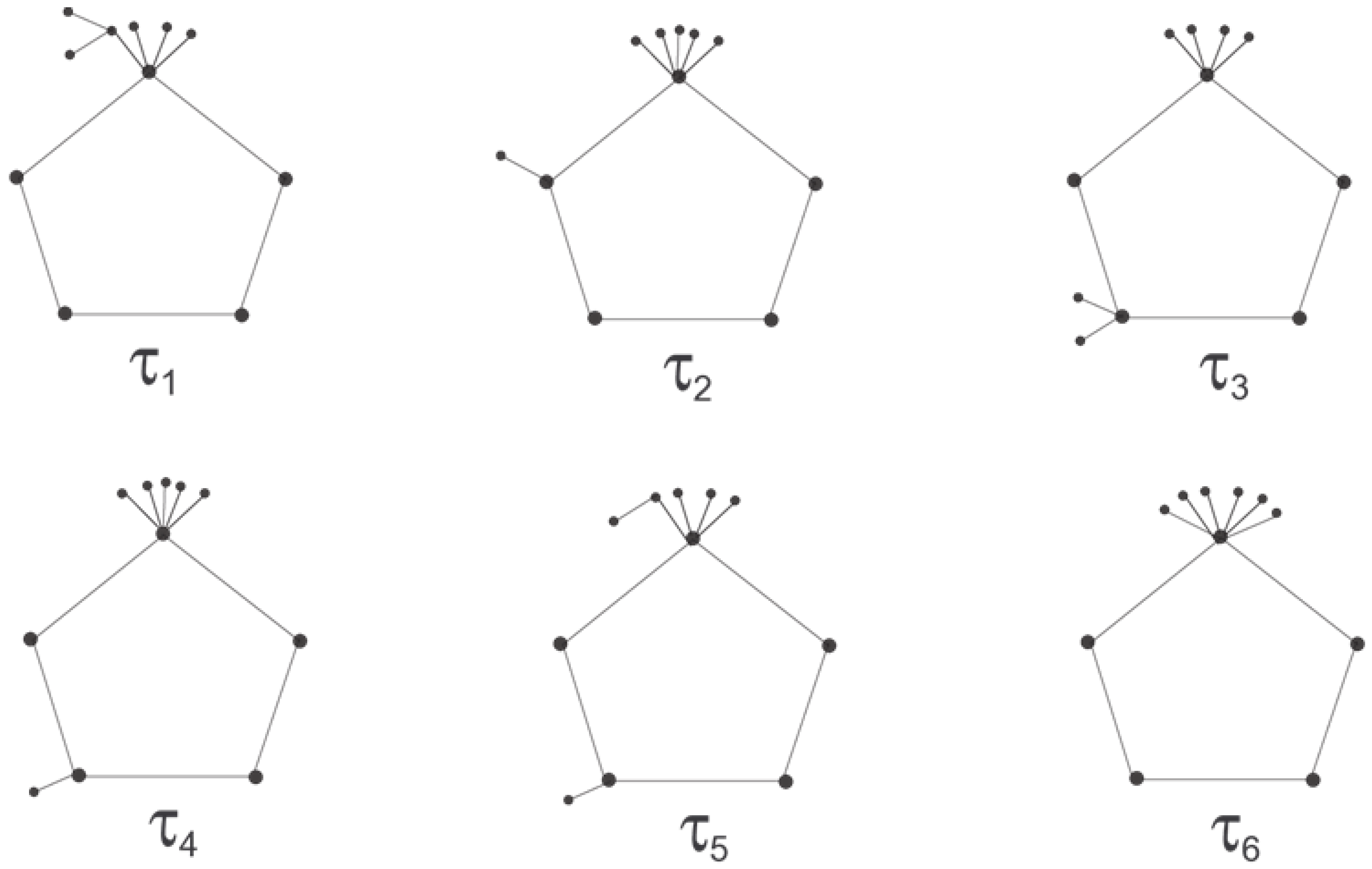
Now we take some graph structures ${\tau }_1,{\tau }_2,{\tau }_3,{\tau }_4,{\tau }_5,{\tau }_6$ with order r = 11 and girth g = 5, shown in Figure 11. Numerical values of Shighalli–Kanabur invariants are shown in

Table 1. Comparison of different values of the SK, SK₁ and SK₂ indices.

Graphic Structure (τ)	SK (τ)	SK1 (τ)	SK2 (τ)
τ1	33	39	109
τ2	38	43.5	143.5
τ3	35	38	115.5
τ4	38	41	141
τ5	33	44	107.5
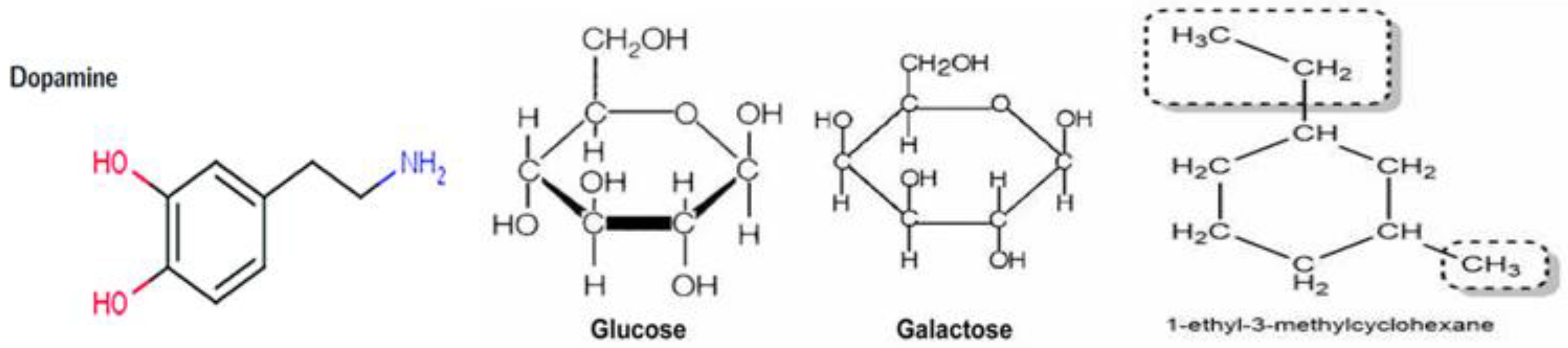
τ6	43	46	183.5

for the above-mentioned graphic structures. We can see that these computations verify our main results in Theorems 3, 6 and 9. We have molecular structures of certain compounds in chemistry which represents some of the graphs of our research as shown in Figure 12.

These structures represents unicyclic graphs having pendant vertices, pendant edges, or pendant paths attached to the vertices of a cycle.

5. Conclusions

In this work, we determined the extremal unicyclic connected graphs of these certain degree-based chemical invariants, i.e., the SK index, the SK₁ index, and the SK₂ index of a given size, order, number of pendant vertices and girth by using some graph transformations. Furthermore, we presented an ordering giving a sequence of unicyclic connected graphs having these indices from greatest in decreasing order.