Chandrasekhar Mass Limit of White Dwarfs in Modified Gravity

Abstract

We investigate the Chandrasekhar mass limit of white dwarfs in various models of $f\left(R\right)$ gravity. Two equations of state for stellar matter are used: the simple relativistic polytropic equation with polytropic index $n=3$ and the realistic Chandrasekhar equation of state. For calculations, it is convenient to use the equivalent scalar–tensor theory in the Einstein frame and then to return to the Jordan frame picture. For white dwarfs, we can neglect terms containing relativistic effects from General Relativity and we consider the reduced system of equations. Its solution for any model of $f\left(R\right)=R+\beta R^m$ ($m\ge 2$, $\beta >0$) gravity leads to the conclusion that the stellar mass decreases in comparison with standard General Relativity. For realistic equations of state, we find that there is a value of the central density for which the mass of a white dwarf peaks. Therefore, in frames of modified gravity, there is a lower limit on the radius of stable white dwarfs, and this minimal radius is greater than in General Relativity. We also investigate the behavior of the Chandrasekhar mass limit in $f\left(R\right)$ gravity.

1. Introduction

Modified gravity in its various forms [1,2,3,4,5,6,7] describes successfully the late-time acceleration of the universe [8,9,10] and provides the possibility to explain also early-time acceleration [11]. Although the most successful model for cosmological acceleration is the $\Lambda$-Cold-Dark-Matter ($\Lambda$CDM) model, it suffers from some difficulties from the fundamental physics viewpoint. Primarily, one needs to explain the so-called cosmological constant problem, i.e., the very large discrepancy between the observed value of the $\Lambda$ term and its value predicted by any quantum field theory [12]. Another way to describe cosmological acceleration in frames of General Relativity (GR) is the introduction of a scalar field. Analysis of Planck observational data leads researchers to the conclusion that such a field may be a phantom field with negative kinetic terms since the parameter of the state equation for dark energy is allowed to have values marginally smaller than $-1$. Phantom fields are very problematic from a quantum field theory perspective.

In modified gravity, we can explain not only data based on standard candles but also anisotropy of microwave background [13], gravitational weak lensing [14], absorption spectrum of Lyman-$\alpha$-line [15] and other phenomena without a cosmological constant or phantom scalars.

However, if we investigate gravitational theories different from General Relativity (GR), we need to consider consequences not only on a cosmological level but also take into account possible manifestations for relativistic astrophysical objects such as white dwarfs, neutron stars and black holes.

In this paper, we consider possible effects of $f\left(R\right)$ gravity in white dwarfs. Models of white dwarfs with polytropic EoS in Palatini $f\left(R\right)$ gravity (without an additional degree of freedom for the gravitational sector) are considered in [16,17]. Early in many papers, another class of compact objects, neutron stars (NS), were considered in connection with modified gravity (see, for instance, [18,19,20,21,22,23,24,25,26,27,28,29,30,31,32,33,34,35,36,37] and a recent review paper [38]). The general feature of the solution of the modified Tolman–Oppenheimer–Volkoff equations is that the scalar curvature R outside the neutron star does not equal zero, as in the Schwarzschild solution, but decreases asymptotically at spatial infinity. The gravitational mass enclosed within the surface of star decreases in comparison with GR for the same central density of matter, but the area around the star with non-zero curvature also contributes to the observed gravitational mass. For a simple $R^2$ gravity effective, the gravitational mass of an NS increases. This result can help explain NSs with large mass [34,35,39,40,41,42,43,44] and therefore gives a realistic description of some phenomena such as the recent GW190814 event.

The density and the scalar curvature in the central areas of white dwarfs are, of course, not so large as those those inside NSs. However, radii of white dwarfs are two or three orders of magnitude larger, and therefore some measurable effect may appear. In Newtonian gravity and for polytropic equation of state equations describing star equilibria, we are given the well-known Lane–Emden equation. From calculations, it follows that we can neglect relativistic effects on a Newtonian background, but it is unknown if this is true for the possible influence of modified gravity. The second important question is the existence of stable stars in modified gravity for realistic EoSs for the branch of stable stellar configurations $dM/d{\rho }_c>0$, where ${\rho }_c$ is central density. As shown in [45], for a relativistic polytropic EoS, gravitational mass decreases with central density for $R^2$ gravity. In the case of Chandrasekhar EoS, mass increases with central density. However, for very high densities (${\rho }_c\sim {10}^{10}$ g/cm${}^3$), this EoS is not applicable. It is interesting to investigate the stability of white dwarfs with this EoS in modified gravity. Since the scalar curvature is relatively small, one can expect that the function $f\left(R\right)$ can be represented as a power series in R. Therefore, we should first consider a simple model of power–law gravity with an additional term $\sim R^l$ for the scalar curvature.

The structure of this paper is as follows: In Section 2 and Section 3, we briefly consider Tolman–Oppenheimer–Volkoff equations in GR and $f\left(R\right)$ gravity. We can neglect relativistic terms for white dwarfs in the first case and obtain the well-known Lane–Emden equation for polytropic EoSs. For $f\left(R\right)$ gravity, the Einstein frame and the corresponding scalar–tensor theory are used for calculations (with a subsequent return to the Jordan frame). Neglecting same relativistic terms, we obtain a reduced system of equations that is easier for numerical analysis. Then, we compare the two approaches to solve this system for simple $R^2$ gravity using a relativistic polytropic EoS with polytropic index $n=3$. Firstly, we can use an approximation for the scalar field. In this case, the scalar field decreases as the density of the star decreases and drops to zero on the star’s surface. Stellar mass decreases in comparison with GR. These results do not change qualitatively if we solve the reduced system without any approximation. The realistic Chandrasekhar EoS is considered in Section 5 for $R^2$ gravity. Finally, we consider the existence of the mass limit for white dwarfs in another model of $f\left(R\right)$ gravity for a polytropic EoS. Assuming a perturbative solution for the scalar field, one can obtain the analog of the Lane–Emden equation and formulate the requirements of the gravity model for which the Chandrasekhar mass limit increases or decreases.

2. Tolman–Oppenheimer–Volkoff Equations in GR

For relativistic non-rotating stars in equilibrium, the following equations should be satisfied:

$$\frac{dm}{dr}=4\pi \rho r^2,$$

(1)

$$\frac{dp}{dr}=-(\rho +p)\frac{m+4\pi p{r}^3}{r^2\left(1-\frac{2m}{r}\right)}.$$

(2)

Here, $\rho$ and p are the density and the pressure of stellar matter, respectively. Function m is the gravitational mass inside a sphere of radius r. Here, we use a natural system of units in which the velocity of light and gravitational constant are $c=G=1$.

For dense matter in white dwarfs, simple polytropic equation of state can be used

$$p=K{\rho }^{1+1/n},$$

(3)

where K, n are constants. For polytropic EoSs, one can obtain simple equations for dimensionless quantities and investigate the properties of the solutions of the TOV equations.

Let us introduce the dimensionless functions $\theta$ and $\mu$ and the coordinate x:

$$\rho ={\rho }_c{\theta }^n,m=\mu {\rho }_c{a}^3,r=ax,$$

where the length parameter a is

$$a={\left(\frac{(n+1)K{\rho }_c^{1/n-1}}{4\pi }\right)}^{1/2}.$$

Therefore, the first equation can be rewritten as

$$\frac{d\mu }{dx}=4\pi x^2{\theta }^n,$$

(4)

and the second equation can be reduced to

$$\frac{1}{1+4\pi \beta \theta /(n+1)}\frac{d\theta }{dx}=-\frac{1}{4\pi }\frac{\mu +16{\pi }^2{(n+1)}^{-1}{x}^3\beta {\theta }^{n+1}}{x(x-2\beta \mu )}.$$

(5)

The dimensionless parameter $\beta$ is

$$\beta ={\rho }_c{a}^2=\frac{n+1}{4\pi }K{\rho }_c^{1/n}<<1,$$

and is very small for the corresponding densities in white dwarfs. If we consider relativistic electrons (${\rho }_c>>{10}^6$ g/cm${}^3$), then $n=3$ and

$$K=1.2435\times {10}^{15}/{\mu }_e^{4/3}$$

in a CGS system. Parameter ${\mu }_e$ is the average molecular weight per one electron. For ${\mu }_e=2$, we have that

$$\beta =3.76\times {10}^{-5}{\left(\frac{{\rho }_c\left[{g/cm}^3\right]}{{10}^7}\right)}^{1/3}$$

If we neglect terms containing $\beta$ in Equations (4) and (5), we obtain the usual Lane–Emden equation:

$$\frac{d}{dx}\left(x^2\frac{d\theta }{dx}\right)=-x^2{\theta }^n.$$

(6)

For a relativistic polytrope with $n=3$, the white dwarf mass does not depend on the density in the center, and $\mu \left(x_f\right)=25.362$ for $x_f=6.896$. This is the Chandrasekhar limit of white dwarf mass $M=1.456M_{\odot }$. By taking into account relativistic terms, the results change negligibly.

3. Spherically Symmetric Stars in f(R)-Gravity

For $f\left(R\right)$ gravity, one needs to replace the standard Einstein–Hilbert action, which contains the scalar curvature R, by some function of curvature $f\left(R\right)$:

$$S=\frac{1}{16\pi }\int d^{4}x\sqrt{-g}f\left(R\right)+S_{\mathrm{matter}}.$$

(7)

$S_{\mathrm{matter}}$ describes the action of standard perfect fluid.

The metric for static stars is spherically symmetric, i.e.,

$$d{s}^2=-e^{2\psi }d{t}^2+e^{2\lambda }d{r}^2+r^{2}d{\Omega }^2,$$

(8)

where $\psi$ and $\lambda$ are two independent functions of r.

For our purposes, it is useful to consider the scalar–tensor theory of gravity, which is equivalent to $f\left(R\right)$ gravity. in the Einstein frame. The corresponding action for the gravitational field is

$$S_g=\frac{1}{16\pi }\int d^{4}x\sqrt{-g}\left(\Phi R-U\left(\mathrm{\Phi }\right)\right),$$

(9)

where the scalar field is $\mathrm{\Phi }=f^{\prime }\left(R\right)$ and the potential is $U\left(\mathrm{\Phi }\right)=R{f}^{\prime }\left(R\right)-f\left(R\right)$. For the redefined metric ${\tilde{g}}_{\mu \nu }=\mathrm{\Phi }{g}_{\mu \nu }$, we rewrite the action as

$$S_g=\frac{1}{16\pi }\int d^{4}x\sqrt{-\tilde{g}}\left(\tilde{R}-2{\tilde{g}}^{\mu \nu }{\partial }_{\mathsf{\mu }}\varphi {\partial }_{\nu }\varphi -4V\left(\varphi \right)\right),$$

(10)

where $\varphi =\sqrt{3}ln\mathrm{\Phi }/2$ and the potential $V\left(\varphi \right)$ is

$$V\left(\varphi \right)={\mathrm{\Phi }}^{-2}\left(\varphi \right)U\left(\mathrm{\Phi }\left(\varphi \right)\right)/4.$$

Intervals in Einstein and Jordan frames are linked by the relation

$$d{\tilde{s}}^2=\mathrm{\Phi }d{s}^2=-e^{2\tilde{\psi }}d{t}^2+e^{2\tilde{\varphi }}{\widetilde{dr}}^2+{\tilde{r}}^{2}d{\Omega }^2.$$

(11)

Here, we write $d{\tilde{s}}^2$ in the form equivalent to (8) but with different functions $\tilde{\psi }$ and $\tilde{\lambda }$.

From Equation (11), we have that ${\tilde{r}}^2=\mathrm{\Phi }{r}^2$ and $e^{2\tilde{\psi }}=\mathrm{\Phi }{e}^{2\psi }$. Combining these with equality

$$\mathrm{\Phi }{e}^{2\lambda }d{r}^2=e^{2\tilde{\lambda }}d{\tilde{r}}^2,$$

we obtain that

$$e^{-2\lambda }=e^{-2\tilde{\lambda }}{\left(1-\tilde{r}{\varphi }^{\prime }\left(\tilde{r}\right)/\sqrt{3}\right)}^2.$$

By analogy with General Relativity, let us define function $m\left(r\right)$ as

$$m\left(r\right)=\frac{r}{2}\left(1-e^{-2\lambda }\right).$$

(12)

Now we need to determine the sense of function $m\left(r\right)$. Analysis of solutions of the modified TOV equations in the case of neutron stars ($R^2$ gravity) shows that scalar curvature quickly drops to zero outside the star (see the results of [30,46,47]), and solutions outside the star behave so that

$$\underset{r\to \infty }{lim}\frac{r}{2}(1-e^{-2\lambda })=M,$$

where M is a constant value. We have, therefore, a solution with a Schwarzschild asymptotic:

$$d{s}^2=-\left(1-\frac{2M}{r}\right)d{t}^2+{\left(1-\frac{2M}{r}\right)}^{-1}d{r}^2+r^{2}d{\Omega }^2.$$

M here is nothing other than gravitational mass measured by an infinitely distant observer. In fact, the solution for outer space for neutron stars in $R^2$ gravity for a reasonable $\alpha$ reconciled with the Schwarzschild solution scales around 10–20 km.

In the case of a white dwarf, we can propose that the solution for outer space is also very close to the Schwarzschild solution already available for some small distances from the star’s surface because values of the gravitational field are smaller in comparison with neutron stars, and therefore, possible deviations from General Relativity should be negligible.

In light of this, it is useful to introduce function $m\left(r\right)$ according to Equation (12) because the asymptotic value of this function gives the gravitational mass of a compact object for a distant observer. If the white dwarf is a component of a binary system, its gravitational mass is defined by an asymptotical value of $m\left(r\right)$.

Let us recall the ADM formalism proposed by R. Arnowitt, S. Deser and C.W. Misner [48]. According to this conception, to define the energy (or mass) in general relativity, one needs to consider the metric tensor at infinity. For asymptotic Minkowski spacetime, one can apply this approach. The ADM energy in the case of such spacetime is defined as a function of the deviation of the metric tensor from its prescribed asymptotic form. Therefore, the ADM energy is calculated as the strength of the gravitational field at spatial infinity.

Obviously, this formalism can be applied to the case of $R^2$ gravity because at spatial infinity, R is so small, and the gravitational field equations coincide with the Einstein equations in GR form.

Finally, we also note an important moment. In General Relativity, the value of $m\left(r\right)$ for $r<r_s$, where $r_s$ is the star’s radius, means the gravitational mass inside a sphere with radius r. For modified gravity, we can also interpret function $m\left(r\right)$ so that outer layers contribute to the gravitational force at distance r. However, we can say that $m\left(r\right)$ is the gravitational mass of a sphere with radius r that will be measured by a sufficiently distant observer in the absence of outer layers for distances greater than r.

Further, we can define function $\tilde{m}\left(\tilde{r}\right)$ by the same relation:

$$\tilde{m}\left(\tilde{r}\right)=\frac{\tilde{r}}{2}\left(1-e^{-2\tilde{\lambda }}\right).$$

Note that function $m\left(r\right)$ can be calculated from $\tilde{m}\left(\tilde{r}\right)$ by using a simple relation

$$m\left(\tilde{r}\right)=\frac{\tilde{r}}{2}\left(1-\left(1-\frac{2\tilde{m}}{\tilde{r}}\right){\left(1-\tilde{r}{\varphi }^{\prime }\left(\tilde{r}\right)/\sqrt{3}\right)}^2\right)e^{-\varphi /\sqrt{3}}.$$

(13)

For $r\to \infty$, dilaton field $\varphi \to 0$, and, therefore, $\tilde{r}\to r$. The asymptotical value of $\tilde{m}\tilde{r}$ coincides with the asymptotical value of $m\left(r\right)$.

For the metric functions, we obtain equations that are very similar to the TOV equations in GR with redefined energy and pressure and with contributions from the scalar field to overall density and pressure $\varphi$ being:

$$\frac{1}{{\tilde{r}}^2}\frac{d\tilde{m}}{d\tilde{r}}=4\pi e^{-4\varphi /\sqrt{3}}\rho +\frac{1}{2}\left(1-\frac{2\tilde{m}}{\tilde{r}}\right){\left(\frac{d\varphi }{d\tilde{r}}\right)}^2+V\left(\varphi \right),$$

(14)

$$\frac{1}{p+\rho }\frac{dp}{d\tilde{r}}=-\frac{\tilde{m}+4\pi e^{-4\varphi /\sqrt{3}}p{\tilde{r}}^3}{\tilde{r}(\tilde{r}-2\tilde{m})}-\frac{\tilde{r}}{2}{\left(\frac{d\varphi }{d\tilde{r}}\right)}^2+\frac{{\tilde{r}}^{2}V\left(\varphi \right)}{\tilde{r}-2\tilde{m}}+\frac{1}{\sqrt{3}}\frac{d\varphi }{d\tilde{r}}.$$

(15)

The second equation is obtained by using the condition of hydrostatic equilibrium:

$$\frac{dp}{d\tilde{r}}=-(\rho +p)\left(\frac{d\psi }{d\tilde{r}}-\frac{1}{\sqrt{3}}\frac{d\varphi }{d\tilde{r}}\right).$$

(16)

For the scalar field, the following equation should be satisfied:

$${▵}_{\tilde{r}}\varphi -\frac{dV\left(\varphi \right)}{d\varphi }=-\frac{4\pi }{\sqrt{3}}{e}^{-4\varphi /\sqrt{3}}(\rho -3p).$$

(17)

Here, ${▵}_{\tilde{r}}$ is the radial part of the Laplace operator for a spherically symmetric metric (11):

$${▵}_{\tilde{r}}=e^{-2\tilde{\lambda }}\left(\frac{2}{r}+\frac{d\psi }{dr}-\frac{d\lambda }{dr}\right)\frac{d}{dr}+e^{-2\tilde{\lambda }}\frac{d^2}{d{r}^2}.$$

We rewrite Equations (14), (15) and (17) in terms of the dimensionless variables introduced earlier:

$$\frac{d\tilde{\mathsf{\mu }}}{dx}=4\pi {\tilde{x}}^2{\theta }^n{\mathrm{e}}^{-4\varphi /\sqrt{3}}+\frac{{\tilde{x}}^2}{\beta }\left(\frac{1}{2}\left(1-\frac{2\beta \tilde{\mathsf{\mu }}}{\tilde{x}}\right){\left(\frac{d\varphi }{d\tilde{x}}\right)}^2+v\left(\varphi \right)\right),$$

(18)

$$\frac{1}{1+4\pi \beta \theta /(n+1)}\frac{d\theta }{d\tilde{x}}=-\frac{1}{4\pi }\frac{\tilde{\mathsf{\mu }}+16{\pi }^2\beta {\theta }^{n+1}{\tilde{x}}^3{e}^{-4\varphi /\sqrt{3}}}{\tilde{x}(\tilde{x}-2\beta \tilde{\mathsf{\mu }})}-$$

(19)

$$-\frac{{\tilde{x}}^2}{4\pi \beta (\tilde{x}-2\beta \tilde{\mathsf{\mu }})}\left(\frac{1}{2}\left(1-\frac{2\beta \tilde{\mathsf{\mu }}}{\tilde{x}}\right){\left(\frac{d\varphi }{d\tilde{x}}\right)}^2-v\left(\varphi \right)\right)+\frac{1}{4\sqrt{3}\pi \beta }\frac{d\varphi }{d\tilde{x}}$$

The variable $v\left(\varphi \right)$ is nothing other than the dimensionless potential, i.e.,

$$v\left(\varphi \right)=a^{2}V\left(\varphi \right).$$

The rewritten equation for the scalar field $\varphi$ is

$$\left(1-\frac{2\beta \tilde{\mathsf{\mu }}}{\tilde{x}}\right)\left(\frac{d^2\varphi }{d{\tilde{x}}^2}+\left(\frac{2}{\tilde{x}}-\frac{4\pi \beta }{1+4\pi \beta /(n+1)}\frac{d\theta }{d\tilde{x}}+\frac{1}{\sqrt{3}}\frac{d\varphi }{d\tilde{x}}\right)\frac{d\varphi }{d\tilde{x}}\right)+$$

(20)

$$+\left(\frac{\beta \tilde{\mathsf{\mu }}}{{\tilde{x}}^2}-\frac{\beta }{\tilde{x}}\frac{d\tilde{\mathsf{\mu }}}{d\tilde{x}}\right)\frac{d\varphi }{d\tilde{x}}-\frac{dv}{d\varphi }=-\frac{4\pi \beta }{\sqrt{3}}{e}^{-4\varphi /\sqrt{3}}{\theta }^n\left(1-12\pi \beta \theta /(n+1)\right).$$

Numerical integration of Equations (18) and (19) with (20) for various n gives the parameter of stellar configuration. From previous analysis of TOV equations for the case of white dwarfs, we know that terms proportional to small parameter $\beta$ do not considerably affect the solution. Assuming the same for the case of modified gravity, we can study the “reduced” system of equations, leaving only terms with a scalar field in which parameter $\beta$ is in the denominator:

$$\frac{d\tilde{\mathsf{\mu }}}{dx}=4\pi {\tilde{x}}^2{\theta }^n{\mathrm{e}}^{-4\varphi /\sqrt{3}}+\frac{{\tilde{x}}^2}{\beta }\left(\frac{1}{2}{\left(\frac{d\varphi }{d\tilde{x}}\right)}^2+v\left(\varphi \right)\right),$$

(21)

$$\frac{d\theta }{d\tilde{x}}=-\frac{\tilde{\mathsf{\mu }}}{4\pi {\tilde{x}}^2}-\frac{\tilde{x}}{4\pi \beta }\left(\frac{1}{2}{\left(\frac{d\varphi }{d\tilde{x}}\right)}^2-v\left(\varphi \right)\right)+\frac{1}{4\sqrt{3}\pi \beta }\frac{d\varphi }{d\tilde{x}}.$$

(22)

In the l.h.s. of Equation (20), we also drop terms containing parameter $\beta$ and terms with the square of the first derivative of the scalar field. In the r.h.s. of this equation, we leave only terms with the first power of $\beta$:

$$\frac{d^2\varphi }{d{\tilde{x}}^2}+\frac{2}{\tilde{x}}\frac{d\varphi }{d\tilde{x}}-\frac{dv}{d\varphi }=-\frac{4\pi \beta }{\sqrt{3}}{e}^{-4\varphi /\sqrt{3}}{\theta }^n.$$

(23)

One should impose the following conditions on unknown variables at the center of a star:

$$\theta \left(0\right)=1,\tilde{\mathsf{\mu }}\left(0\right)=0,\varphi \left(0\right)={\varphi }_0,\frac{d\varphi \left(0\right)}{d\tilde{x}}=0.$$

The condition of asymptotic flatness requires that

$$\varphi \to 0atx\to \infty .$$

We investigate the solution of the system of equations in the Einstein frame and then go back to the physical frame. We are mainly interested in the effects of modified gravity, and therefore, we consider a reduced system of Equations (21)–(23).

4. Simple Model of R²-Gravity: Perturbative Approach and Numerical Integration of Reduced System

Considering simple $R^2$ gravity with $f\left(R\right)=R+\alpha R^2$ gravity, we have that

$$v\left(\varphi \right)=\frac{1}{16\tilde{\alpha }}{\left(1-e^{-2\varphi /\sqrt{3}}\right)}^2,\tilde{\alpha }=\alpha /a^2.$$

(24)

Usually, one assumes that $\alpha >0$, otherwise the model of $R^2$ gravity leads to instabilities. Because the scalar field is very small, we can expand the potential $v\left(\varphi \right)$, leaving only the first non-zero term:

$$v\left(\varphi \right)=\frac{1}{12\tilde{\alpha }}{\varphi }^2.$$

Assuming $v\left(\varphi \right)$ is dominant and $\varphi$ is very small, we can reduce Equation (23) to the relation between the density and the scalar field:

$$\frac{\varphi }{6\tilde{\alpha }}=\frac{4\pi \beta }{\sqrt{3}}{\theta }^n.$$

(25)

From this approximation, it follows that outside the star, $\varphi =0$ and $\frac{d\varphi }{dx}=0$. Therefore, ${\tilde{x}}_f=x_f$ and $\tilde{\mathsf{\mu }}\left({\tilde{x}}_f\right)=\mathsf{\mu }\left(x_f\right)$.

From observations of relativistic binaries [49], it follows that the upper limit on parameter $\alpha$ is $\sim {10}^{15}$ cm${}^2$. For $\alpha ={10}^{14}$ cm${}^2$, the results of the calculations are given in

Table 1. Differences between results for stellar masses from exact solutions of reduced system (M) and perturbative solution ($M_p$) for $\alpha ={10}^{14}$ cm${}^2$. We also provide corresponding values of dimensionless parameter $\tilde{\alpha }$ and the relation ${\varphi }_c/{\varphi }_p\left(0\right)$. Here, ${\varphi }_c$ is the value of $\varphi$ at $r=0$, and ${\varphi }_p\left(0\right)$ is the value of the scalar field from the perturbative approximation.

$ln{\mathit{\rho }}_{\mathit{c}}$	$\tilde{\mathit{\alpha }},$	${\mathit{\varphi }}_{\mathit{c}}/{\mathit{\varphi }}_{\mathit{p}}\left(0\right)$	$\mathit{M},$	${\mathit{M}}_{\mathit{p}},$
	${\mathbf{10}}^{-\mathbf{3}}$		${\mathit{M}}_{\odot }$	${\mathit{M}}_{\odot }$
7	1.97	∼1	1.448	1.448
7.5	4.25	∼1	1.439	1.439
8	9.15	0.92203	1.419	1.418
8.5	19.71	0.76707	1.389	1.377
9	42.48	0.62547	1.334	1.295
9.5	91.52	0.46316	1.260	1.162

.

The analysis shows that the contribution of the scalar field on the pressure and the density is very negligible. Only the last term in (22) gives a considerable effect on the solution of the equations. It is very easy to understand why this happens. From the approximation (25), it follows that $d\varphi /dx\sim \alpha \mathcal{O}\left(\beta \right)$, and therefore,

$$\frac{1}{2}{\left(\frac{d\varphi }{dx}\right)}^2\sim {10}^2{\tilde{\alpha }}^2\mathcal{O}\left({\beta }^2\right),v\left(\varphi \right)\sim 10\tilde{\alpha }\mathcal{O}\left({\beta }^2\right).$$

The length parameter a varies from $2.25\times {10}^8$ cm for ${\rho }_c={10}^7$ g/cm${}^3$ to $4.85\times {10}^7$ cm for ${\rho }_c={10}^9$ g/cm${}^3$. Therefore, even for the upper limit of the parameter $\alpha$, the dimensionless parameter $\tilde{\alpha }<1$, and the contribution of the terms in brackets in (21) and (22) is $\mathcal{O}\left(\beta \right)$, i.e., it is comparable with the relativistic effects from General Relativity in comparison with Newtonian gravity.

Only for sufficiently large $\tilde{\alpha }$ can one expect that the approximation (25) does not work; this is because the square of the scalar field derivative is then comparable to the value of the potential term.

We investigated solutions of the reduced system of equations without approximation (25) and found that using the more exact solution for the scalar field increases the mass of the star. For $\tilde{\alpha }<0.02$, this increase is less than $0.01M_{\odot }$ in comparison to the perturbative solution. In the case of $\alpha ={10}^{14}$ cm${}^2$, this corresponds to central densities up to $3.2\times {10}^8$ g/cm${}^3$. For $\alpha ={10}^{13}$ cm${}^2$, the approximation (25) can be used for central densities ${\rho }_c<{10}^{10}$ g/cm${}^3$. In real white dwarfs, it is assumed that central densities are less. For $\alpha ={10}^{15}$ cm${}^2$, one needs to solve the exact equation for the scalar field. Of course, such values of parameter $\alpha$ represent only a theoretical interest because the decrease in white dwarf mass is very large in comparison with GR, which is difficult to reconcile with available observational data.

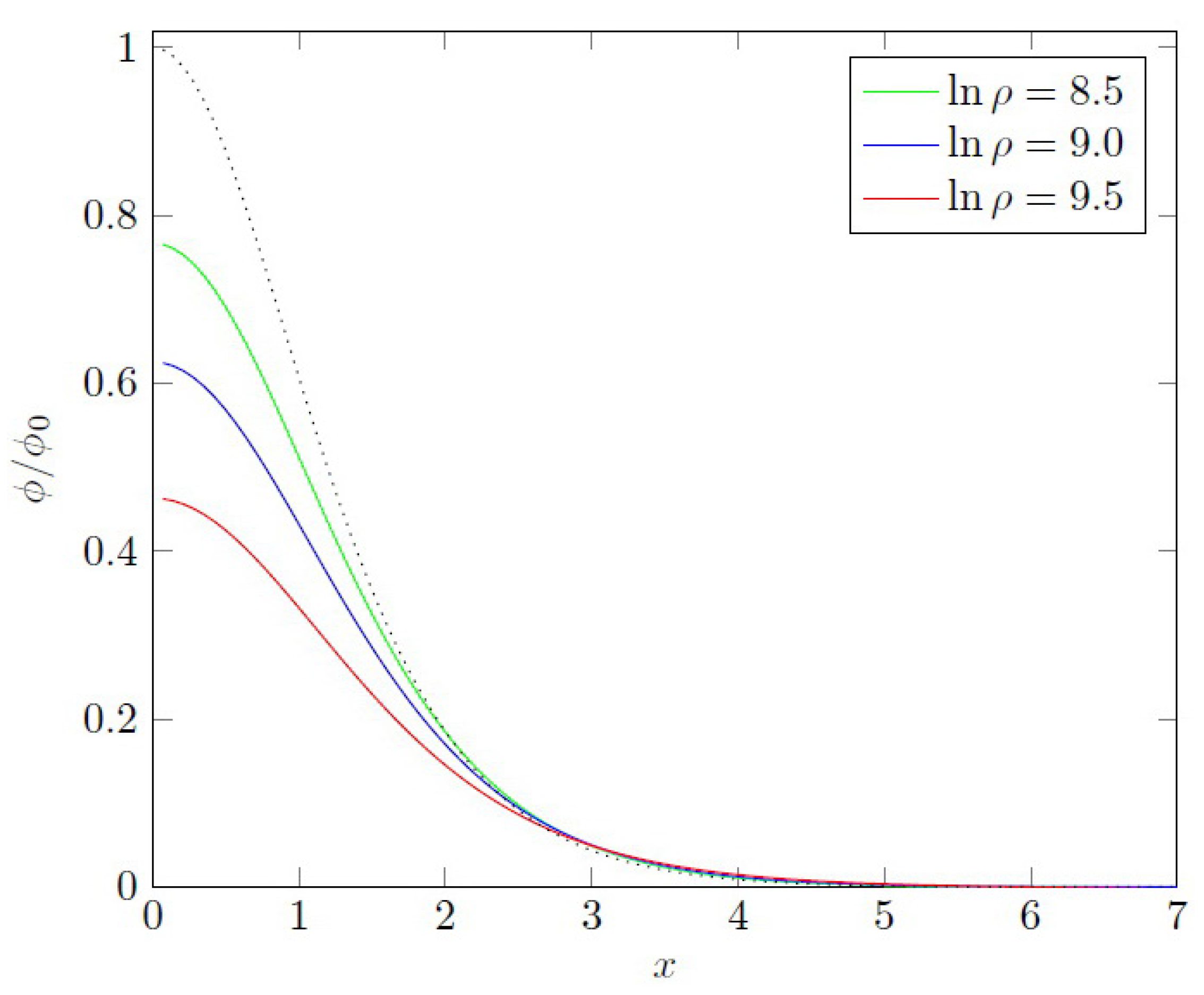
The profile of the scalar field from the solution of (23) is a function that decreases with coordinate x and follows the density profile. For illustration, we plot the solution of (23) and the profile of the scalar field derived from (25) for various values of ${\rho }_c$ and $\alpha ={10}^{14}$ cm${}^2$ (see Figure 1). For large $\tilde{\alpha }$, the profile of the exact solution differs significantly from the approximation. We also see that the “tail” of the scalar field outside the star’s surface is very short and that this existence does not affect the stellar mass. We point out that another situation takes place in neutron stars. Density sharply drops near the surface of an NS, but the scalar field decreases more slowly, and therefore, in $R^2$ gravity around the surface of a neutron star, a “gravitational sphere” exists with scalar curvature $R\ne 0$ (or $\varphi \ne 0$ in the Einstein frame). This contributes to the gravitational mass, and for high central densities and $\alpha >0$, NS mass increases.

5. Realistic Equation of State

The next step is to consider more-realistic EoSs. We choose the Chandrasekhar EoS for stellar matter, which can be written in parametric form:

$$\rho =B{y}^3,$$

(26)

$$p=A\left[y(2y^2-3){(1+y^2)}^{1/2}+3ln(x+{(1+x^2)}^{1/2}\right],$$

$$B=9.82\times {10}^5{\mu }_e{g/cm}^3,A=6.02\times {10}^{22}{dyne/cm}^2.$$

Again, it is useful to introduce dimensionless variables in Equations (14) and (15). Taking into account characteristic radii and masses of white dwarfs, let us define:

$$\tilde{r}=R_e\tilde{x},\tilde{m}=M_{\odot }\tilde{\mathsf{\mu }},$$

$$\rho ={\rho }_c\eta ,p=p_c\xi .$$

Here, $R_e$ means the radius of the Earth. Restoring G and c in the equations, we derive the following equations for dimensionless variables $\tilde{\mathsf{\mu }}$, $\eta$, $\xi$ and $\varphi$:

$$\frac{d\tilde{\mathsf{\mu }}}{d\tilde{x}}=\delta 4\pi {\tilde{x}}^2{e}^{-4\varphi /\sqrt{3}}\eta +\frac{1}{2}\frac{R_e}{r_g}\left(1-\frac{2r_g}{R_e}\frac{\tilde{\mathsf{\mu }}}{\tilde{x}}\right){\left(\frac{d\varphi }{d\tilde{x}}\right)}^2+\frac{R_e}{r_g}v\left(\varphi \right),$$

(27)

$$\frac{1}{\eta +\xi /\gamma }\frac{d\xi }{d\tilde{x}}=-\gamma \frac{r_g}{R_e}\frac{\tilde{\mathsf{\mu }}}{\tilde{x}(\tilde{x}-2r_g\tilde{\mathsf{\mu }}/R_e)}-\delta \frac{r_g}{R_e}\frac{4\pi e^{-4\varphi /\sqrt{3}}{\tilde{x}}^3\xi }{\tilde{x}(\tilde{x}-2r_g\tilde{\mathsf{\mu }}/R_e)}+$$

(28)

$$+\gamma \left(-\frac{\tilde{x}}{2}{\left(\frac{d\varphi }{d\tilde{x}}\right)}^2+\frac{{\tilde{x}}^{2}v\left(\varphi \right)}{\tilde{x}-2r_g\tilde{\mathsf{\mu }}/R_e}+\frac{1}{\sqrt{3}}\frac{d\varphi }{d\tilde{x}}\right),$$

$$\left(1-\frac{2r_g}{R_e}\frac{\tilde{\mathsf{\mu }}}{\tilde{x}}\right)\left(\frac{d^2\varphi }{d{\tilde{x}}^2}+\left(\frac{2}{\tilde{x}}-\frac{1}{\gamma \eta +\xi }\frac{d\xi }{dx}+\frac{1}{\sqrt{3}}\frac{d\varphi }{d\tilde{x}}\right)\frac{d\varphi }{d\tilde{x}}\right)+$$

(29)

$$+\frac{r_g}{R_e}\left(\frac{\tilde{\mathsf{\mu }}}{{\tilde{x}}^2}-\frac{1}{\tilde{x}}\frac{d\tilde{\mathsf{\mu }}}{d\tilde{x}}\right)\frac{d\varphi }{d\tilde{x}}-\frac{dv}{d\varphi }=-\frac{4\pi \delta }{\sqrt{3}}\frac{r_g}{R_e}{e}^{-4\varphi /\sqrt{3}}\left(\eta -3\xi /\gamma \right),$$

where the dimensionless parameters $\delta$ and $\gamma$ are introduced:

$$\delta =\frac{{\rho }_c{R}_e^3}{M_{\odot }},\gamma =\frac{{\rho }_c{c}^2}{p_c}$$

and $v\left(\varphi \right)=V\left(\varphi \right)R_e^2$. The parameter $r_g=G{M}_{\odot }/c^2$. Again, we consider the reduced system of equations, neglecting terms containing the relation $r_g/R_e<<1$ in the denominators and taking into account that the parameter $\gamma >>\delta$ for white dwarfs, and we get

$$\frac{d\tilde{\mathsf{\mu }}}{d\tilde{x}}=\delta 4\pi {\tilde{x}}^2{e}^{-4\varphi /\sqrt{3}}\eta +\frac{R_e}{r_g}\left({\left(\frac{1}{2}\frac{d\varphi }{d\tilde{x}}\right)}^2+v\left(\varphi \right)\right),$$

(30)

$$\frac{1}{\eta }\frac{d\xi }{d\tilde{x}}=-\gamma \frac{r_g}{R_e}\frac{\tilde{\mathsf{\mu }}}{{\tilde{x}}^2}+\gamma \left(-\frac{\tilde{x}}{2}{\left(\frac{d\varphi }{d\tilde{x}}\right)}^2+\tilde{x}v\left(\varphi \right)+\frac{1}{\sqrt{3}}\frac{d\varphi }{d\tilde{x}}\right),$$

(31)

$$\frac{d^2\varphi }{d{\tilde{x}}^2}+\left(\frac{2}{\tilde{x}}+\frac{1}{\sqrt{3}}\frac{d\varphi }{d\tilde{x}}\right)\frac{d\varphi }{d\tilde{x}}-\frac{dv}{d\varphi }=-\frac{4\pi \delta }{\sqrt{3}}\frac{r_g}{R_e}{e}^{-4\varphi /\sqrt{3}}\eta .$$

(32)

As in the previous case, we consider the potential for $R^2$ gravity and compare results from the perturbative approximation of the scalar field and the more exact solution of (32). The main result is the same as for the relativistic polytrope: the stellar mass decreases in comparison with GR for the same central density. For large densities, the perturbative approximation is not valid. However, in the case of $R^2$ gravity, the stellar mass has a maximum for some central density, and then the mass decreases, although in GR, the mass grows with density for the Chandrasekhar EoS.

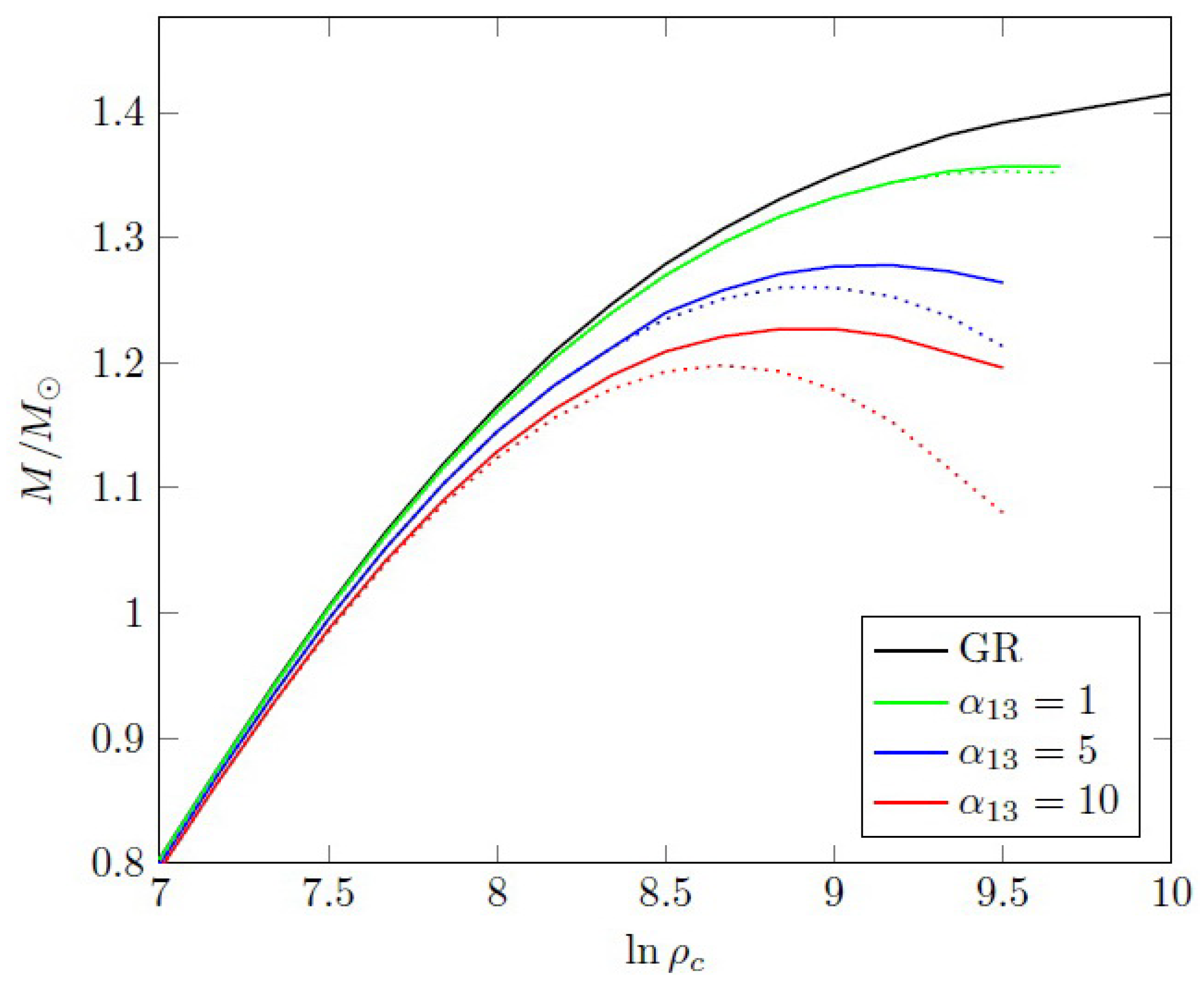
In Figure 2, we depict the mass–density relation for the interval of densities between ${10}^7$ and ${10}^{10}$ g/cm${}^3$ for various values of $\alpha$. These results are important for establishing the upper limit of parameter $\alpha$ in $R^2$ gravity. According to the latest observations, white dwarfs with masses $M>1.3M_{\odot }$ are very rare [50]. The most massive white dwarf is J1329 + 2549 with a mass of $1.351\pm 0.006M_{\odot }$. Considering $1.35M_{\odot }$ as the lower limit of the maximal value for white dwarf mass and assuming that the Chandrasekhar EoS is valid, we conclude that $\alpha <{10}^{13}$ cm${}^2$. Analyzing white dwarf radii and masses in $R^2$ gravity for realistic values of $\alpha$ can be performed using the approximation of the scalar field.

From our results, it follows that for ${\rho }_c>{\rho }_c^{crit}$, white dwarfs are unstable in $R^2$ gravity. The critical density and minimal radius of a white dwarf depends on the value of $\alpha$. In light of these results for masses and radii of white dwarfs near the Chandrasekhar limit, one can define the upper limit of $\alpha$ more precisely.

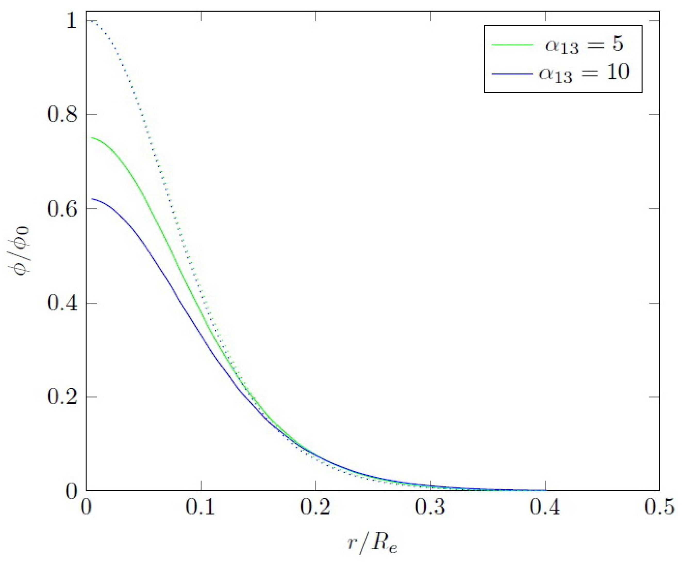
The scalar field obtained from the numerical solution of Equations (30)–(32) decreases from the center to the surface of the star in the same manner as for the case of a polytropic EoS: it starts from $\varphi \left(0\right)<{\varphi }_0$, where ${\varphi }_0$ is the central value of the perturbative solution, and then it follows the density profile (see Figure 3).

6. Chandrasekhar Limit of Mass in Another Model of Modified Gravity

We showed that in the case of white dwarfs in $R^2$ gravity with realistic parameters, we can neglect the derivatives of the scalar field in its field equation and use a simple approximation for $\varphi$. As we showed, the profile of the scalar field is a monotonic function of the radial coordinate. It is interesting to investigate another model of modified gravity.

Let us consider a model with $f\left(R\right)=R+{\alpha }^{l-1}{R}^l$, where $l>2$. This representation is chosen so that parameter $\alpha$ has a dimension of the square of length. The potential of the scalar field theory in the corresponding equivalent scalar–tensor theory in this case is

$$V\left(\mathrm{\Phi }\right)=D{\mathrm{\Phi }}^{-2}{\left(\mathrm{\Phi }-1\right)}^{\frac{l}{l-1}},D=\frac{l-1}{4l^{\frac{l}{l-1}}}{\alpha }^{-1},\mathrm{\Phi }=e^{2\varphi /\sqrt{3}}.$$

(33)

Again, for very small values of scalar field $\varphi$, one can expand the expression for $V\left(\varphi \right)$ and obtain

$$V\left(\varphi \right)\approx D{\left(\frac{2}{\sqrt{3}}\right)}^{\frac{l}{l-1}}{\varphi }^{\frac{l}{l-1}}.$$

If the potential term dominates, we can use approximation

$$\varphi \approx \frac{l{\left(2\sqrt{3}\right)}^l}{4}{\left(\frac{\alpha }{a^2}\right)}^{l-1}{\left(\frac{4\pi \beta }{\sqrt{3}}\right)}^{l-1}{\theta }^{n(l-1)}.$$

(34)

The dimensionless potential and the square of the scalar field derivative are, in order of magnitude,

$$v\left(\varphi \right)\sim {\left(\frac{\alpha }{a^2}\right)}^{l-1}\mathcal{O}\left({\beta }^l\right),{\left(\frac{d\varphi }{dx}\right)}^2\sim {\left(\frac{\alpha }{a^2}\right)}^{2(l-1)}\mathcal{O}\left({\beta }^{2l-2}\right).$$

One can expect that for realistic values of $\alpha /a^2<<1$, approximation of the scalar field is valid. Further, as in the case of $R^2$ gravity, the effects of the scalar field on the density and the pressure are negligible. Moreover, for $m\ge 3$, the effects of modified gravity are of the next order of smallness on parameter $\beta$ in comparison with the relativistic effects of GR in the background of Newton’s gravity. The square of the scalar field derivative is an order lower in comparison with the potential term for $l>2$.

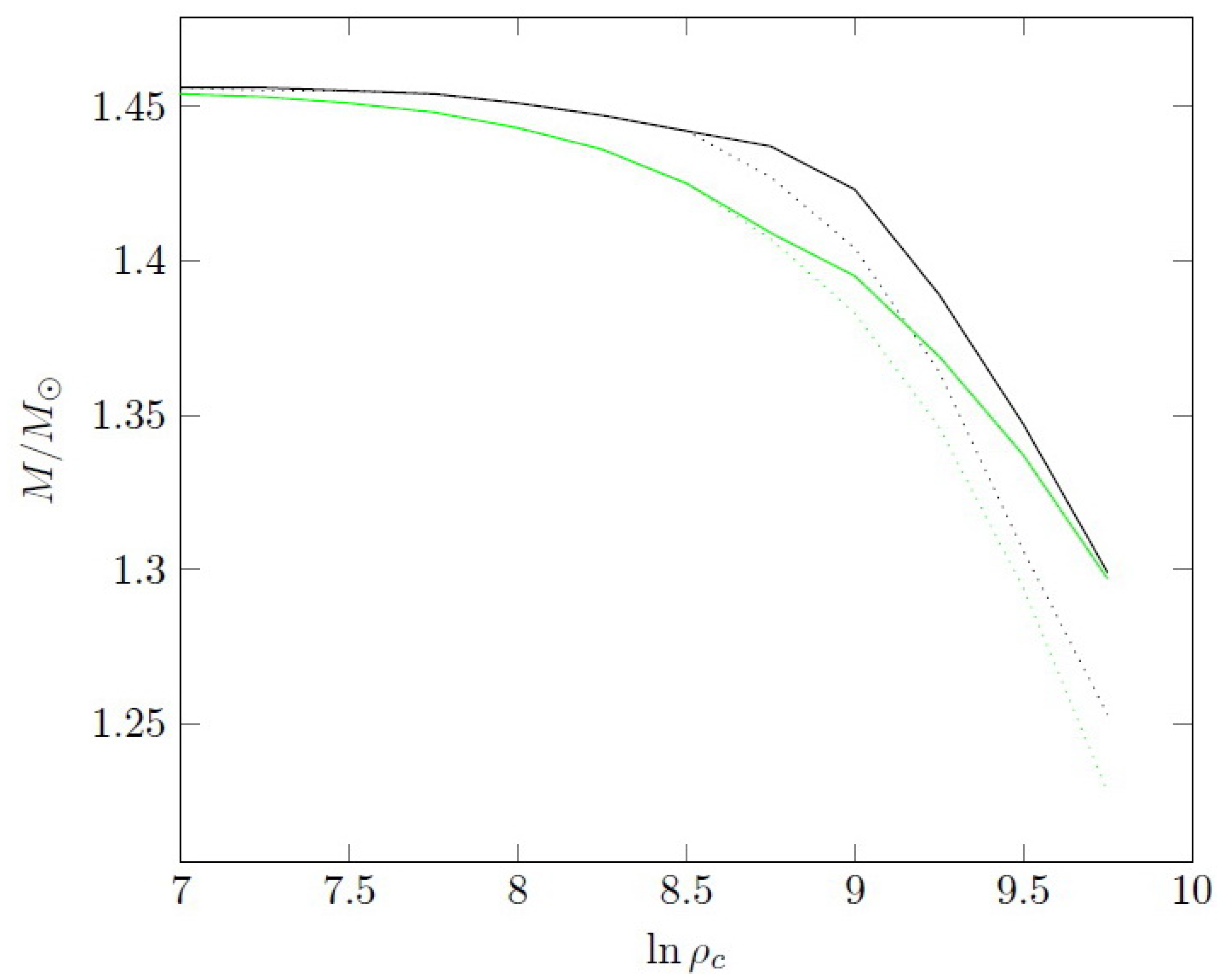
Calculations for some $l>2$ show the same pattern as for $l=2$: the star mass decreases with increasing central density. Some results are given in Figure 4. For $\alpha /a^2\sim \mathcal{O}\left(1\right)$, the perturbative solution is not valid. Obviously, for a realistic Chandrasekhar EoS, we obtain that the stellar mass has a maximum for a certain density.

If we assume that the perturbative approximation for the scalar field is valid, then the scalar field is a monotonic function of $\varphi$ because $dv/d\varphi >0$, as follows from relation

$$\frac{dv}{d\varphi }=\frac{4\pi \beta }{\sqrt{3}}{\theta }^n.$$

(35)

Of course, $\theta$ is a monotonically decreasing function of coordinates for stable stellar configurations. Therefore, for the scalar field, we can write that

$$\varphi =F\left(\theta \right)$$

where F is a monotonic increasing function of its argument. The scalar field decreases with the coordinate, and the potential tends to its minimum on the star’s surface. The following conditions should be imposed on function F:

$$F\left(\theta \right)=0,\frac{dF}{d\theta }=0for\theta =0.$$

(36)

These conditions guarantee that the scalar field and its first derivative outside the star vanish. Of course, for many potentials of the scalar field, we cannot explicitly obtain that a relationship between $\varphi$ and $\theta$ exists. The first derivative of the scalar field is

$$\frac{d\varphi }{d\tilde{x}}=\frac{dF}{d\theta }\frac{d\theta }{d\tilde{x}}.$$

Equation (22), by taking into account the expression for the derivative of the scalar field and without the term ${(d\varphi /dx)}^2$, can be written as

$$\left\{1-\frac{1}{4\sqrt{3}\pi \beta }\frac{dF}{d\theta }\right\}\frac{d\theta }{dx}=-\frac{\tilde{\mathsf{\mu }}}{4\pi {\tilde{x}}^2}+\frac{\tilde{x}}{4\pi \beta }v\left(\varphi \right).$$

(37)

Then after some simple algebra, one obtains the analog of the Lane–Emden equation:

$$\frac{d}{d\tilde{x}}\left\{{\tilde{x}}^2\left\{1-\frac{1}{4\sqrt{3}\pi \beta }\frac{dF}{d\theta }\right\}\frac{d\theta }{dx}\right\}=-{\tilde{x}}^2{\theta }^n{e}^{-4\varphi /\sqrt{3}}+\frac{{\tilde{x}}^2}{2\pi \beta }v\left(\varphi \right)+\frac{{\tilde{x}}^3}{\sqrt{3}}{\theta }^n\frac{dF}{d\theta }\frac{d\theta }{d\tilde{x}}.$$

(38)

To obtain the scalar field potential as a function of $\theta$ in the frame of our approximation, one needs to take the following integral:

$$v\left(\theta \right)=\frac{4\pi \beta }{\sqrt{3}}{\int }_0^{\theta }\frac{dF}{d\theta }{\theta }^{n}d\theta .$$

(39)

Therefore, for a given $F\left(\theta \right)$, we obtain the potential in parametric form. Of course, the explicit form of $v\left(\varphi \right)$ can be written only for relatively simple functions $F\left(\theta \right)$. The function $\tilde{\mathsf{\mu }}$ is defined from the following relation:

$$\tilde{\mathsf{\mu }}\left(x\right)=-4\pi {\tilde{x}}^2\frac{d\theta \left(\tilde{x}\right)}{d\tilde{x}}+\frac{{\tilde{x}}^3}{\beta }v\left(\theta \right)+\frac{{\tilde{x}}^2}{\sqrt{3}\beta }\frac{dF}{d\theta }\frac{d\theta \left(\tilde{x}\right)}{d\tilde{x}}.$$

(40)

Realistic solutions of Equation (38) for a chosen $F\left(\theta \right)$ posses the same property as the solution of the Lane–Emden equation in Newtonian gravity: for some ${\tilde{x}}_f$, the function $\theta$ vanishes. This ${\tilde{x}}_f$ corresponds to the surface of the white dwarf. In the Jordan frame, $x_f={\tilde{x}}_f$ because scalar field $\varphi$ is zero on the star’s surface, and therefore, $\mathrm{\Phi }=1$. Because the first derivative of the scalar field also vanishes on the surface, the gravitational mass of a white dwarf is

$$\mu =\tilde{\mathsf{\mu }}\left({\tilde{x}}_f\right)$$

and therefore,

$$\mu =-4\pi {\tilde{x}}_f^2\frac{d\theta \left({\tilde{x}}_f\right)}{d\tilde{x}}$$

because $v\left(\theta \right)=0$ and $dF/d\theta =0$ for $\theta =0$.

Because the curvature R in the case of white dwarfs is relatively small, one can propose that $f\left(R\right)$ can be represented as series in powers of R:

$$f\left(R\right)=R+{\alpha }_1{R}^2+{\alpha }_2^2{R}^3+...$$

For $R\to 0$ and ${\alpha }_1\ne 0$, the corresponding potential of the equivalent scalar–tensor theory is

$$v\left(\varphi \right)\to \frac{{\varphi }^2}{12{\alpha }_1}.$$

If ${\alpha }_2\ne 0$ and ${\alpha }_1=0$, the potential $v\left(\varphi \right)\sim {\varphi }^{3/2}$, and so on. Therefore, the first derivative of potential $dv/d\varphi$ should contain terms $\sim {\varphi }^{1/(k-1)}$, $k=2,3...,$ and the monotonic function $F\left(\theta \right)$ is a sum

$$F\left(\theta \right)=s_1{\theta }^n+s_2{\theta }^{2n}+...$$

on interval $0\le \theta \le 1$. From previous results, we conclude that stellar mass decreases for this function $F\left(\theta \right)$ with increasing central density. Therefore, in the frame of the perturbative approach for realistic $f\left(R\right)$, one should expect that the mass of the white dwarf decreases in comparison with the GR case for the same central density.

If the function $F\left(\theta \right)$ decreases with its argument, this corresponds to an increasing scalar field $\varphi$ from the center to the surface. If the scalar field is defined from (35), this leads to an increase in the potential term from the center to the surface. For $R^2$ gravity, such a situation takes place for $\alpha <0$. However, this model of gravity cannot be considered realistic because it leads to instabilities.

Therefore, we conclude that in the frame of a perturbative approach, it is impossible to construct solutions of the system (21)–(23) such that gravitational mass increases in comparison with GR. Increases in the value take place only for unrealistic models of $F\left(R\right)$ gravity.

A non-monotonic function $F\left(\theta \right)$, as follows from (39), leads to the potential of the scalar field being an ambiguous function of its argument. We consider if a solution of (23) exists such that the derivative of the scalar field changes the sign. Let us assume that this indeed happens once. The scalar field starts from some positive value at the center of the star and reaches a minimum ${\varphi }_{min}<0$ at some point $x_s$. At the vicinity of the minimum $d^2\varphi /d{x}^2\ge 0$ and, therefore, $dv/d\varphi >0$; the potential goes down. Then, the scalar field increases and asymptotically tends to zero for large x. The asymptotical value of the scalar field outside the star should correspond to the minimum of the potential. We have, therefore, the situation, which, for example, can take place for potentials of the form $u\sim {\varphi }^n$, where $n=2k$, $k=1,2...$ The scalar field reaches the minimum for some $x<x_s$ and develops negative values and finally approaches zero and again the minimum of the potential. However, our consideration shows that for such potentials, we can construct solutions when the scalar field is a monotonic decreasing function from center to surface.

7. Concluding Remarks

We investigated the question of the maximal white dwarf mass limit in $f\left(R\right)$ gravity. Our analysis involved a polytropic EoS with $n=3$ and a more-realistic Chandrasekhar EoS. Additionally, the equivalent scalar–tensor theory in the Einstein frame was used, with a subsequent transition to the Jordan picture. For $f\left(R\right)$ gravity, one can consider the reduced system of equations because relativistic effects of GR in the case of white dwarfs are negligible in the Newtonian gravity background. In models with $f\left(R\right)=R+{\alpha }^{l-1}{R}^l$, for any $l\ge 2$, the mass of white dwarfs decreases in comparison with GR for ${\alpha }^{l-1}>0$. For realistic values of $\alpha$, the perturbative approach is valid. It is sufficient to account for only potential terms in the equation for the scalar field and obtain a relation for its field. For stable stars, the density should decrease from the center to the surface, and the corresponding profile of the scalar field also decreases. It is important to note that the contribution of the scalar field to energy density is around $\mathcal{O}\left({\beta }^{l-1}\right)$, where $\beta ={\rho }_c{a}^{2}G/c^2$ is a small relativistic parameter. This contribution is comparable (for $R^2$ gravity) with the effect from the relativistic corrections to solutions of the Lane–Emden equation or even less (for $l>2$). Applicability of the perturbative approach is defined by the relation ${(\alpha /a^2)}^{l-1}$. More-precise calculations show that the scalar field starts from some value $\kappa {\varphi }_p\left(0\right)$ at the center of the star, where $0<\kappa <1$, and ${\varphi }_p\left(0\right)$ is the central value of the scalar field from approximation. Our main result is that, in the case of f(R) gravity for a realistic equation of state, a limit of mass exists for some central density. For ${\rho }_c>{\rho }_0$, mass decreases. For GR in the case of the Chandrasekhar EoS, $M\to M_{max}$ for $\rho \to \infty$ (of course this limit is formal because, in reality, white dwarf densities in every case are so far from the densities of neutron stars). Precise estimations of the maximal value of white dwarf mass from astronomical observations has significance for constraining the upper limit of parameter $\alpha$. If the Chandrasekhar EoS is valid, we can reconcile observational data for white dwarfs in $R^2$ gravity only for $\alpha <{10}^{13}$ cm${}^2$. In comparison with NSs, it is worth noting that, as believed, the EoS is known to be much more accurate. Therefore, one can hope that the possible effects of modified gravity will not be disguised by uncertainty in the knowledge of the equation of state. For NSs, the solution of the scalar field also has the following feature, namely around the area of the star for which $\varphi \ne 0$ exists: this area contributes to the gravitational mass, and the net effect for neutron mass with masses $M>1.5M_{\odot }$ is an increasing in mass. For white dwarfs, there are no significant “scalar tails”, because near the surface, the perturbative solution is valid with high accuracy, and therefore, the scalar field is mainly defined by density. In the Einstein frame, this means that scalar curvature near the surface is close to its value in GR, namely $R\approx 8\pi (\rho -3p)$, and drops to zero outside the star very quickly.

In conclusion, we note one more interesting point. White dwarfs, as well known, are progenitor stars of SNIa type supernovae, which are considered standard candles. We question if the effects of modified gravity on the Chandrasekhar mass would affect the interpretation of SNIa supernovae as standard candles. The detailed answer requires, of course, numerical analysis of the physics of an SNe explosion. As we mentioned in the text of paper, the maximal mass of a white dwarf from observation in any case is $1.35$ or more solar masses, i.e., it is very close to the canonical Chandrasekhar limit (1.44 solar masses). We propose that if the luminosity of an SNe is a little less than it is for the canonical limit, one needs to slightly reconsider luminosity distances for candles to the side of decreasing them. Therefore, in principle, this may lead to some corrections to the energy budget of the universe (relation between the densities of dark energy and matter). However, it is unlikely that this correction is very large and goes beyond a few percent.