Viability of Baryon to Entropy Ratio in Modified Hořava–Lifshitz Gravity

Abstract

In this paper, we study the matter–antimatter imbalance in the universe through baryogenesis (also known as baryosynthesis), which is a physical process that took off just a little while after the big bang explosion, producing a supremacy of matter over antimatter. In this work, we commit the reproduction of the baryon to entropy ratio ($\frac{{\eta }_{{}_B}}{S}=\frac{{\eta }_{{}_{\beta }}-{\eta }_{\overline{{}_{\beta }}}}{S}$), where ${\eta }_{{}_{\beta }}\left({\eta }_{\overline{{}_{\beta }}}\right)$ is a baryon(anti-baryon) number and S is the entropy of the universe in the presence of modified Hořava-Lifshitz $F\left(R\right)$ gravity, which is also called $F\left(\tilde{R}\right)$-gravity. We inspect different baryogenesis interactions proportional to $\tilde{R}$ (where $\tilde{R}$ is the argument of general function F used for the development of modified Hořava-Lifshitz gravity). For this study, we examine two models by choosing different values of $F\left(\tilde{R}\right)$. In the first model, the functional value of $F\left(\tilde{R}\right)=\tilde{R}+\alpha {\tilde{R}}^2$ (where $\alpha$ is a real constant). The second model is more generalized and extended as compare to first one. Mathematically, this model is given by $F\left(\tilde{R}\right)=\tilde{R}+\alpha {\tilde{R}}^2+\beta {\tilde{R}}^m$, where $\alpha$, $\beta$ are real constants and $m>2$ is a real model parameter. Our results for both models and different values of m point out that matter-antimatter asymmetry does not vanish under the effect of the modified Hořava-Lifshitz theory of gravity, which shows a consistent and compatible fact of gravitational baryogenesis with recent observational data.

1. Introduction

In our universe, the supremacy of matter over antimatter has been one of the great puzzles since cosmology became a sovereign research field. The data observed from a cosmic microwave background (CMB) [1], assisting with the big bang nucleosynthesis (BBN) [2], revealed the supremacy of matter over antimatter in the universe. Physicists believe that just a little while after the explosion, an asymmetry appeared between matter and antimatter, which changed a minute part of antimatter into matter. Then, matter and antimatter annihilated, which caused a surplus amount of matter which is considered as all matter that can we observe and that exists around us. However, it is not yet revealed why this asymmetry (called “baryon asymmetry”) comes to exist. The cosmological theories that make an effort to resolve this fundamental query lie under the realm of baryogenesis (a process that took place at the birth time of the universe and produced more matter then antimatter). Among these, one theoretically attractive mechanism for initiating the matter–antimatter asymmetry is “gravitational baryogenesis” [3]. The other similar theories which addressed baryogenesis are black hole (BH) evaporation baryogenesis [4], Affleck-Dine baryogenesis [5], grand-unified-theory (GUT) baryogenesis [6], electroweak baryogenesis [7], and spontaneous baryogenesis [8,9]. All of these theories are committed to clarify why this kind of asymmetry exists in the cosmos. Observational data [1,2] provide a confirmation that $\frac{{\eta }_{{}_B}}{S}$ is nearly equal to $9.42\times {10}^{-11}$, where S denotes the universe entropy while ${\eta }_{{}_B}$ represents the baryon number.

Gravitational baryogenesis [3] is one such theory that played a vital role in the modification and extension of various modified theories of gravity [10,11,12,13]. Half a century ago, Sakharove [14] discussed three major conditions that must be met to create more matter then antimatter, which are: (i) baryon number violation, (ii) charge (C) and charge-parity ($\mathcal{CP}$) symmetry are violated, and (iii) the process occurs out of thermal inequilibrium. The gravitational baryogenesis mechanism utilizes one of Sakharov’s conditions and the baryon–anti-baryon asymmetry was assured by the existence of the $\mathcal{CP}$ violation (violation of conservation laws related to the charge conjugation and parity by the weak force). It is given by a change in the Ricci scalar and coupling between the baryon current $J^i$, as

$$\begin{array}{c}\hfill \frac{1}{M_{*}^2}\int \sqrt{-g}\left({\partial }_{i}R\right)J^i{d}^{4}x,\end{array}$$

(1)

where $M_{*}$ is the parameter characterizing the cutoff scale of the underlying effective gravitational theory, g is the determinant of the metric tensor, $J^i$ describes baryonic matter current, and R represents the Ricci scalar. Under the effect of flat (Friedmann–Robertson-Walker) FRW metric, we obtain $\frac{{\eta }_B}{S}\propto \dot{R}$, where the overhead dot represents the time rate of change. Physicists further extended Equation (1) to many modified theories of gravity [10,15,16]. The reason behind the extension of this interaction to modified theories is deduced from the fact that other curvature invariants such as the Gauss–Bonnet (GB) scalar $\mathcal{G}$, torsion scalar $\mathbb{T}$, and non-metricity Q produce a non-zero baryon asymmetry with $\omega =1/3$ (radiation-dominated universe), which cannot be obtained in general relativity (GR). For the modified Hořava-Lifshitz $f\left(\tilde{R}\right)$-gravity, the relation for the $\mathcal{CP}$-violating interaction is

$$\begin{array}{c}\hfill \frac{1}{M_{*}^2}\int \sqrt{-g}\left({\partial }_i\tilde{R}\right)J^i{d}^{4}x.\end{array}$$

(2)

Some physicists have also worked on Hořava-Lifshitz gravity as well as on some other modified gravity theories and found viable results [17,18,19,20,21,22,23,24,25,26,27,28,29,30,31,32,33]. An extension of the baryogenesis phenomenon is discussed by many physicists, considering various modified theories of gravity, which are established by the modification in the Einstein–Hilbert action. The suitable and interesting modification in these theories of gravity is the curvature-based formulation of GR. A promising modification in which torsional formulation took the place of the curvature scalar is teleparallel gravity. Lagrangian density in the framework of this gravity supports the Weitzenböck connection instead of the torsionless Levi-Civita. Further, the generalized function $f\left(\mathbb{T}\right)$ is used instead of the torsion scalar $\mathbb{T}$ to obtain a generalized form of this theory, called $f\left(\mathbb{T}\right)$-gravity. In the same manner, $f\left(R\right)$-gravity can be constructed by taking the scalar curvature R into account instead of the Lagrangian density as an extension of teleparallel gravity. It is important that $f\left(R\right)$ and $f\left(\mathbb{T}\right)$ represent different modification classes, which assures one that these theories are not coincidental to each other.

Nojiri and Odintsov have strived to review modified theories of gravity and concluded a rich cosmological structure [34]. It is observed that these theories provide evidence of a transition to the accelerated expansion phase of the universe and may pass the solar system test. In [35], both strong and weak gravitational backgrounds of $f\left(R\right)$-gravities are considered to discuss inflation, dark energy (DE), cosmic perturbation, and local gravity constraints. The authors in [36] discussed the different representation and properties of the $f\left(R\right)$-gravity and its modified form. It is found that numerous DE models with different fluids may imitate the $\Lambda$CDM model consistency with the recent observational bounds [37].

The study of gravitational baryogenesis emerged from the near past and many scientists investigated it while considering various theories of gravity. Bento et al. [38] investigated the effect of the well-known term $\frac{{\eta }_B}{S}$ in the context of the GB braneworld cosmology. This phenomenon is studied under the effect of the $f\left(R\right)$-gravity in [15]. Oikonomou [39] studied the gravitational baryogenesis mechanism for a Type IV singularity, considering two distinct models that described two different Type IV singularities. Considering various cases of $f\left(\mathbb{T}\right)$-gravity, Oikonomou and Saridakis [11] have discussed baryogenesis. It is observed for the loop quantum cosmology (LQC) [40] that $\frac{{\eta }_B}{S}$ is consistent with observational data. The same authors examined baryon number to entropy ratio for the GB gravitational baryogenesis term [10]. The investigation of gravitational baryogenesis, considering the $f\left(R\right)$-gravity, with nonminimal coupling between matter and curvature, is focused in [12]. Considering that the universe is composed of DE and perfect fluid, this ratio is discussed for $f(R,\mathcal{T})$ gravity [41], where $\mathcal{T}$ is the trace of the energy momentum tensor. The results obtained by them was well matched with observational data. Sahoo and Bhattacharjee [13] discussed the baryogenesis phenomenon for the non-minimal $f(R,\mathcal{T})$ gravity and obtained well-matched outcomes with observational bounds.

Bhattacharjee and Sahoo [16] investigated baryogenesis in the $f(Q,\mathcal{T})$ gravity and concluded that this gravity is consistent with the gravitational baryogenesis phenomenon. Consistent results with observational data are extracted for the baryon to entropy ratio by Bhattacharjee [42], taking non-minimal $f\left(\mathbb{T}\right)$ and $f(\mathbb{T},B)$ theories of gravity into account, where B is the boundary term. Azhar et al. [43] considered the power law scale factor to discuss the generalized gravitational baryogenesis for $f(\mathbb{T},{\mathbb{T}}_G)$ and $f(\mathbb{T},B)$ gravity models and verify the consistency of results with observations (where ${\mathbb{T}}_G$ is the teleparallel equivalent to the GB term). Agrawal et al. [44] considered the matter field to be made up with perfect fluid to discuss the gravitational baryogenesis models comparison in $f\left(R\right)$ gravity. Azhar et al. [45] examined baryogenesis in the context of $f(\mathcal{G},\mathcal{T})$ and $f(R,\mathcal{G})$, using some specific models to evaluate the term $\frac{{\eta }_B}{S}$, such as $f(\mathcal{G},\mathcal{T})=\delta {\mathcal{G}}^m+\lambda \mathcal{T}$ and $f(\mathcal{G},\mathcal{T})=\delta {\mathcal{G}}^m+\mathcal{T}+ϵ{\mathcal{T}}^2$. The outcomes from these models exhibit such values which lie in the range of observational data. The models discussed for the $f(R,\mathcal{G})$ gravity were $f(R,\mathcal{G})=k_{1}R+k_2{R}^n{\mathcal{G}}^m$ and $f(R,\mathcal{G})=f_{o}R+f_1\sqrt{\mathcal{G}}$, and they found consistent results with observations. Mavromatos [46] used the string/brane theory through the compactification of spatial dimensions in the presence of non-trivial Kalb-Ramond axion-like fields, which have not been fully explored so far. He discussed a scenario which produced a spontaneous Lorentz and CPT-violating cosmological backgrounds, which in the early universe can lead to baryogenesis through leptogenesis which can be initiated from the idea of baryogenesis in models with heavy right-handed neutrinos. Jawad and Sultan [47] investigated the matter–antimatter asymmetry in context of $f(R,A)$ cosmology, where A is the trace of anti-curvature, and found compatible outcomes with recent observational data.

The aim and motivation of this work is to investigate the implication of modified Hořava-Lifshitz $F\left(R\right)$ gravity to address the phenomenon of gravitational baryogenesis, which came into existence along with the big bang, by discussing the coupling time $t=t_D$, a prerequisite to examining this physical aspect of the universe. Since one among the biggest difficulties towards quantum theories of gravity is that GR is non-renormalizable which causes a loss of theoretical control and predictability at high energies. In 2009, Hořava presented a new theory avoiding this issue by invoking a Lifshitz-type anisotropic scaling at high energy [48] due to which it is called Hořava-Lifshitz theory of gravity. The casual structure of this theory was depending on foliation theory and relativistic concept of time emerges at large distances. Mathematically, this theory is considered as topologically massive theory that involves the Cotton tensor which is a feasible ultra violet (UV) completion of GR where at high energies speed of light goes to infinity. The quality of this approach comparing to previous quantum gravity approaches such as LQC is that it uses concepts from condensed matter physics such as quantum critical phenomena. Due to importance of this theory, its various important cosmological implications have investigated. For example, in early universe it leads to regular bounce solutions due to higher spatial curvature term [49,50] which is also a source to milder the flatness problem [51]. The horizon problem is addressed with anisotropic scaling of the theory and leads to a scale- invariant cosmological perturbations without inflation [52]. Circularly polarized gravitational waves can be generated by considering parity-violating version of this theory [53].

Since, modified Hořava-Lifshitz theory of gravity addressed the issues of renormalizability and UV divergence by rejecting Lorentz asymmetry. The basic idea to evade the above issue is invoking a different kind of scaling in the UV which is anisotropic scaling also called Lifshitz scaling. Mathematically this scaling can be given as

$$\begin{array}{c}\hfill t\to b^{z}t,\overrightarrow{x}\to bx,\varphi \to b^{-s}\varphi ,\end{array}$$

where $\varphi$ represents scalar field, the number z is called dynamical critical exponent, b is an arbitrary number and s gives the scaling dimension which may be given as

$$\begin{array}{c}\hfill z+3-2z-2s=0.\end{array}$$

Here z comes from $dt$, 3 from $d^3\overrightarrow{x}$, $-2z$ from two times derivatives and $-2s$ from two $\varphi$’s in the canonical kinetic term which leads to the relation

$$\begin{array}{c}\hfill s=\frac{3-z}{2}.\end{array}$$

It is interesting that $z=3$ implies $s=0$ which means that the amplitude of quantum fluctuations of $\varphi$ does not change as the energy scale of the system changes for which details are given in [54]. Moreover, this theory has answered questions about the major issues of modern cosmology (i.e., accelerated expansion). Therefore, we are motivated to investigate whether the modified Hořava-Lifshitz theory of gravity confirms the occurrence of the gravitational baryogenesis scenario, which is the source for the existence of baryon asymmetry in the universe.

The layout of paper is as follows: in Section 2, we provide a summary of the $f\left(\tilde{R}\right)$-gravity and discuss field equations for the theory. We also discuss the argument $\tilde{R}$ in this section that is utilized for Friedmann equations. In Section 3, we explain the phenomenon of the gravitational baryogenesis scenario and study it for modified Hořava-Lifshitz gravity in detail. In Section 4, we present the viability of the term $\frac{{\eta }_B}{S}$ for the model $f\left(\tilde{R}\right)=\tilde{R}+\alpha {\tilde{R}}^2$. In Section 5, we describe the baryogenesis scenario in order to examine its viability with observational data for another model $f\left(\tilde{R}\right)=\tilde{R}+\alpha {\tilde{R}}^2+\beta {\tilde{R}}^m$. In Section 6, we conclude our results.

2. Modified Hořava-Lifshitz Gravity

The generalized action term for modified Hořava-Lifshitz gravity is given by [55,56]

$$\begin{array}{c}\hfill S_{F\left(\tilde{R}\right)}=\int d^{4}x\sqrt{-g}F\left(\tilde{R}\right)+S_m,\end{array}$$

(3)

where $\sqrt{-g}=\sqrt{g^{\left(3\right)}}N$, N, depending on time t, is called the lapse function and $S_m$ is the matter’s part of the action. Moreover,

$$\begin{array}{c}\hfill \tilde{R}=K_{ab}{K}^{ab}-\lambda K^2+2\mu {\nabla }_{\sigma }(n^{\sigma }{\nabla }_{\nu }{n}^{\nu }-n^{\nu }{\nabla }_{\nu }{n}^{\sigma })-{\mathcal{L}}_R^{\left(3\right)}\left(g_{ab}^{\left(3\right)}\right).\end{array}$$

(4)

Here $\lambda$, $\mu$ are real constants, ${\mathcal{L}}_R^{\left(3\right)}$ is a function depending on the three-dimensional metric $g_{ab}^{\left(3\right)}$ and the covariant derivatives ${\nabla }_a^{\left(3\right)}$ are defined by this metric, $n^{\sigma }$, which is a unit vector perpendicular to the three-dimensional hypersurface, $K=K_a^a$, and $K_{ab}$ describes the extrinsic curvature, which can be given as $K_{ab}=\frac{1}{2N}\left({\dot{g}}_{ab}^{\left(3\right)}-{\nabla }_a^{\left(3\right)}{N}_b-{\nabla }_b^{\left(3\right)}{N}_a\right)$ [55]. For the FRW universe, line element is given by

$$\begin{array}{c}\hfill d{s}^2=-N^{2}d{t}^2+a{\left(t\right)}^2\left[\frac{d{r}^2}{1-\kappa r}+r^2(d{\theta }^2+si{n}^2\theta d{\varphi }^2)\right],\end{array}$$

(5)

where $a=a\left(t\right)$ is the scale factor of the universe and $\kappa$ curvature parameter while $\kappa =-1,0,1$ represents the open, flat, and closed universe, respectively [57]. We consider the flat FRW universe ($\kappa =0$) to be composed with perfect fluid. The energy momentum tensor for such a case is given by $T_{ab}=p{g}_{ab}+(\rho +p)U_a{U}_b$, where $\rho$ is the total energy density of the system, p describes the total pressure of the universe and $U_a$ is called the four-velocity. The continuity equation for modified Hořava-Lifshitz gravity in a standard form is given by $\dot{\rho }+3H(\rho +p)=0$, where $H=\frac{\dot{a}}{a}$ is called the Hubble parameter. In this scenario, the argument $\tilde{R}$ takes the form

$$\begin{array}{c}\hfill \tilde{R}=\frac{(3-9\lambda )H^2}{N^2}+\frac{6\mu }{a^{3}N}\frac{d}{dt}\left(\frac{H{a}^3}{N}\right).\end{array}$$

(6)

Here, t is cosmic time (laterally, in our work, this cosmic time t will be dealt as the coupling time, $t_D$). If we choose parameters $\lambda =\mu =1$ with a flat FRW universe, then $\tilde{R}$ reduces to R, and hence the usual $f\left(R\right)$-gravity is obtained. If we select $\mu =0$, $\tilde{R}$ reduces to $R_{HL}$ (Ricci scalar for Hořava-Lifshitz gravity) [56] and thus the action (3) becomes similar to the action term of Hořava-Lifshitz-like $f\left(R\right)$-gravity [58]. Hence, this assumption ($\mu =0$) conforms to a degenerate limit of the general $f\left(R\right)$ Hořava-Lifshitz theory of gravity. We call this limit degenerate, as it is very difficult to obtain (it might be impossible).

Considering the FRW cosmology for action (3), the spatial curvature $R_{ab}^{\left(3\right)}=R^{\left(3\right)}$ vanishes; thus, ${\mathcal{L}}_R^{\left(3\right)}$ does not contribute anything. In other words, the same FRW cosmology is obtained for any choice of ${\mathcal{L}}_R^{\left(3\right)}$. It is obvious that this situation varies when BH or solutions with a non-trivial dependence are considered. Suppose that the universe is composed with perfect fluid, varying (3) with regards to $g_{ab}^{\left(3\right)}$ and setting $N=1$; the Friedmann equations for modified Hořava-Lifshitz gravity are given by

$$\begin{array}{ccc}\hfill \rho & =& F\left(\tilde{R}\right)-6\left[(1-3\lambda +3\mu )H^2+\mu \dot{H}\right]F^{\prime }\left(\tilde{R}\right)+6\mu H\frac{d{F}^{\prime }\left(\tilde{R}\right)}{dt}-\frac{c}{a^3},\hfill \\ \hfill p& =& -F\left(\tilde{R}\right)+2\left[(1-3\lambda +3\mu )(\dot{H}+3H^2)\right]F^{\prime }\left(\tilde{R}\right)+2(1-3\lambda )H\frac{d{F}^{\prime }\left(\tilde{R}\right)}{dt}\hfill \end{array}$$

(7)

$$\begin{array}{ccc}\hfill & -& 2\mu \frac{d^2{F}^{\prime }\left(\tilde{R}\right)}{d{t}^2},\hfill \end{array}$$

(8)

where the prime denotes the derivative of the respective function with respect to the argument. Here, c is the constant of integration. One can find $c=0$ [56], but it has been claimed in [59] that c will not always vanish in a local region. In the region where $c>0$, the term $c{a}^{-3}$ may be considered as dark matter (DM). Latterly, we consider both cases of c to analyze the scenario of gravitational baryogenesis. The value of the argument $\tilde{R}$ from Equation (6) reduces to

$$\begin{array}{c}\hfill \tilde{R}=3(1-3\lambda +6\mu )H^2+6\mu \dot{H}.\end{array}$$

(9)

3. Gravitational Baryogenesis

According to the observational data, such as CMB [1] and BBN [2], the numeric value observed for baryogenesis in different models is [16,45]

$$\begin{array}{c}\hfill \frac{{\eta }_{{}_B}}{S}\simeq 9.42\times {10}^{-11}.\end{array}$$

(10)

Modern cosmology is of the opinion that there will be produced an equal amount of matter and antimatter if an explosion occurs which results no baryon but the current observational scheme [1,2], and without intense matter-antimatter annihilation [60], it is strongly recommended that there is more matter than antimatter in the universe. The total amount of this asymmetry is proposed by these observational schemes and is defined by the dimensionless parameter

$$\begin{array}{c}\hfill \eta =\frac{{\eta }_{{}_B}}{S}=\frac{{\eta }_{{}_{\beta }}-{\eta }_{\overline{{}_{\beta }}}}{S}.\end{array}$$

(11)

This baryon asymmetry gives rise to gravitational baryogenesis. As the universe became cool during its evolution and gained in temperature less then the critical temperature $T_D$ (the universe temperature at which the baryon asymmetry-generating interactions arise), which is usually represented by ${T|}_{T_D}$, the asymmetry existing in the cosmos is nearly equal to [3]

$$\begin{array}{c}\hfill \frac{{\eta }_{{}_B}}{S}\simeq -\frac{15g_{{}_b}}{g_{*s}}\frac{\dot{R}}{M_{*}^{2}T}{|}_{T_D},\end{array}$$

(12)

where $g_{{}_b}\sim \mathcal{O}\left(1\right)$ is the number representing the intrinsic degree of freedom of the baryons and $g_{*s}$ represents the total degree of freedom for those particles, which contributes to the entropy of the universe, adopting very close values to the total degree of freedom of massless particles [15] i.e., $g_{*s}=g_{*}\simeq 106$.

To discuss the baryogenesis, we consider that the system prevails in the thermal equilibrium. Moreover, at each state of the universe, the energy density corresponding to temperature T yields

$$\begin{array}{c}\hfill \rho \left(T\right)=\frac{{\pi }^2}{30}{g}_{*s}{T}^4.\end{array}$$

(13)

Hence, the related ratio $\frac{{\eta }_{{}_B}}{S}$ for the $\mathcal{CP}$-violating interaction terms of Equation (2) takes the form as

$$\begin{array}{c}\hfill \frac{{\eta }_B}{S}\simeq -\frac{15g_{{}_b}}{g_{*s}}\frac{\dot{\tilde{R}}}{M_{*}^{2}T}{|}_{T_D}.\end{array}$$

(14)

It would be useful to consider the power law solution to calculate the term $\frac{{\eta }_B}{S}$ under the action of modified Hořava-Lifshitz gravity for different models, because such kinds of solutions are supportive to elaborate all cosmic modification such as radiation, DE-, and DM-dominated eras. We assume a power law solution for each model in the context of modified Hořava-Lifshitz gravity. The scale factor of the universe for the power law model is give by [55,61]

$$\begin{array}{c}\hfill a\left(t\right)=a_0{t}^n,H\left(t\right)=\frac{n}{t},\tilde{R}=\frac{3n(n-3\lambda n+6\mu n-2\mu )}{t^2},\end{array}$$

(15)

where n is a positive real number and $a_0$ is the value of the scale factor at the current time. Inserting $\dot{\tilde{R}}$ from the above equation in (14) and after simplifications yields

$$\begin{array}{c}\hfill \frac{{\eta }_{{}_B}}{S}\simeq \frac{45n(n-3\lambda n+6\mu n-2\mu )g_b}{2{\pi }^2{g}_{*s}{M}_{*}^2{T}_D}{t}^{-3}.\end{array}$$

(16)

4. Model: I

This section is devoted to discuss the phenomenon of gravitational baryogenesis for modified Hořava-Lifshitz gravity, for which we suppose $F\left(\tilde{R}\right)$ in Equation (7) to be as [56]

$$\begin{array}{c}\hfill F\left(\tilde{R}\right)=\tilde{R}+\alpha {\tilde{R}}^2,\end{array}$$

(17)

where $\alpha$ is a real constant. Differentiating Equation (17) with respect to $\tilde{R}$ and substituting the value of $\tilde{R}$ from (15), we obtain

$$\begin{array}{c}\hfill F^{\prime }\left(\tilde{R}\right)=1+\frac{6\alpha n(n-3\lambda n+6\mu n-2\mu )}{t^2},\end{array}$$

(18)

which yields

$$\begin{array}{ccc}\hfill \frac{d{F}^{\prime }\left(\tilde{R}\right)}{dt}& =& -\frac{12\alpha n(n-3\lambda n+6\mu n-2\mu )}{t^3}.\hfill \end{array}$$

(19)

Substituting the values from (13), (15), (17)–(19) in (7), the simplification leads to

$$\begin{array}{ccc}\hfill t^4-\frac{90n}{{\pi }^2{g}_{*s}{T}_D^4}(3\lambda n-n& -& 4\mu )t^2-\frac{270\alpha n}{{\pi }^2{g}_{*s}{T}_D^4}(n-3\lambda n+6\mu n-2\mu )(n^2-3\lambda n^2\hfill \\ \hfill & +& 6\mu n^2-14\mu n+12\lambda -12\mu -4)+\frac{30c}{a_o^3{\pi }^2{g}_{*s}{T}_D^4}=0.\hfill \end{array}$$

(20)

Solving this equation for t, we obtain four different solutions, among which three do not satisfy the observational bounds for $\frac{{\eta }_{{}_B}}{S}$ and look like extraneous roots of the model. The only solution of Equation (20), which gives good results for $\frac{{\eta }_{{}_B}}{S}$, is given by

$$\begin{array}{ccc}\hfill t& =& \left[\frac{1}{2}\right(\frac{8100n^2}{{\pi }^4{g}_{*s}^2{T}_D^8}{(n-3\lambda n+4\mu )}^2-\frac{120}{{\pi }^2{g}_{*s}{T}_D^4}(\frac{c}{a^3}-81\alpha {\lambda }^2{n}^4+324\alpha \lambda \mu n^4\hfill \\ \hfill & +& 54\alpha \lambda n^4-324\alpha {\mu }^2{n}^4-108\alpha \mu n^4-432\alpha \lambda \mu n^3+864\alpha {\mu }^2{n}^3+144\alpha \mu n^3\hfill \\ \hfill & +& 324\alpha {\lambda }^2{n}^2-972\alpha \lambda \mu n^2-9\alpha n^4-216\alpha \lambda n^2+396\alpha {\mu }^2{n}^2+324\alpha \mu n^2\hfill \\ \hfill & +& 216\alpha \lambda \mu n+36\alpha n^2-216\alpha {\mu }^{2}n-72\alpha \mu n){)}^{\frac{1}{2}}+\frac{135\lambda n^2-45n^2-180\mu n}{{\pi }^2{g}_{*s}{T}_D^4}{]}^{\frac{1}{2}}.\hfill \end{array}$$

(21)

As cosmic time t gives rise to the coupling time $t_D$, the above Equation (21) becomes as

$$\begin{array}{ccc}\hfill t_D& =& \left[\frac{1}{2}\right(\frac{8100n^2}{{\pi }^4{g}_{*s}^2{T}_D^8}{(n-3\lambda n+4\mu )}^2-\frac{120}{{\pi }^2{g}_{*s}{T}_D^4}(\frac{c}{a^3}-81\alpha {\lambda }^2{n}^4+324\alpha \lambda \mu n^4\hfill \\ \hfill & +& 54\alpha \lambda n^4-324\alpha {\mu }^2{n}^4-108\alpha \mu n^4-432\alpha \lambda \mu n^3+864\alpha {\mu }^2{n}^3+144\alpha \mu n^3\hfill \\ \hfill & +& 324\alpha {\lambda }^2{n}^2-972\alpha \lambda \mu n^2-9\alpha n^4-216\alpha \lambda n^2+396\alpha {\mu }^2{n}^2+324\alpha \mu n^2\hfill \\ \hfill & +& 216\alpha \lambda \mu n+36\alpha n^2-216\alpha {\mu }^{2}n-72\alpha \mu n){)}^{\frac{1}{2}}+\frac{135\lambda n^2-45n^2-180\mu n}{{\pi }^2{g}_{*s}{T}_D^4}{]}^{\frac{1}{2}}.\hfill \end{array}$$

(22)

Replacing t by $t_D$ and substituting the above value in Equation (16), we obtain

$$\begin{array}{ccc}\hfill \frac{{\eta }_{{}_B}}{S}& \simeq & \frac{45n(n-3\lambda n+6\mu n-2\mu )g_b}{2{\pi }^2{g}_{*s}{M}_{*}^2{T}_D}\left[\frac{1}{2}\right(\frac{8100n^2}{{\pi }^4{g}_{*s}^2{T}_D^8}{(n-3\lambda n+4\mu )}^2-\frac{120}{{\pi }^2{g}_{*s}{T}_D^4}\hfill \\ \hfill & \times & (\frac{c}{a^3}-81\alpha {\lambda }^2{n}^4+324\alpha \lambda \mu n^4+54\alpha \lambda n^4-324\alpha {\mu }^2{n}^4-108\alpha \mu n^4-9\alpha n^4\hfill \\ \hfill & -& 432\alpha \lambda \mu n^3+864\alpha {\mu }^2{n}^3+144\alpha \mu n^3+324\alpha {\lambda }^2{n}^2-972\alpha \lambda \mu n^2-216\alpha \lambda n^2\hfill \\ \hfill & +& 396\alpha {\mu }^2{n}^2+324\alpha \mu n^2+36\alpha n^2+216\alpha \lambda \mu n-216\alpha {\mu }^{2}n-72\alpha \mu n){)}^{\frac{1}{2}}\hfill \\ \hfill & +& \frac{135\lambda n^2-45n^2-180\mu n}{{\pi }^2{g}_{*s}{T}_D^4}{]}^{-\frac{3}{2}},\hfill \end{array}$$

(23)

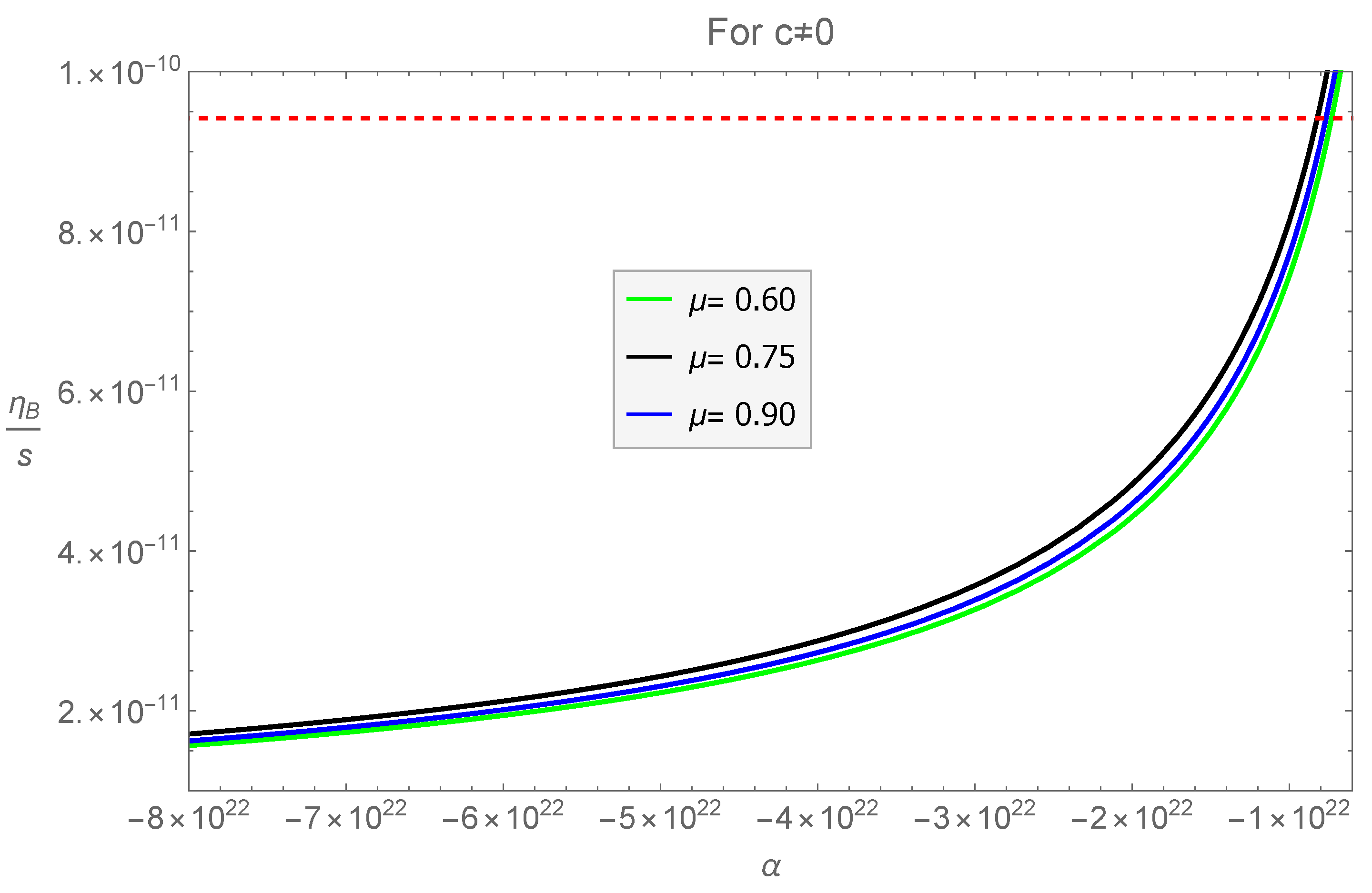
In Figure 1, $\frac{{\eta }_B}{S}$ has been plotted versus parameter $\alpha$ for different values of parameter $\mu =0.60,0.75,0.90$, which belongs to real numbers. For this evaluation, the integration constant c in Equation.(7) is taken to be non-zero (i.e., $c=0.3$) and the other parameters are $a_0=1$, $g_{{}_b}=1$, $g_{*s}=106$, $\lambda =0.7$, $M_{*}={10}^{12}$ GeV, $n=0.5$, and $T_D=2\times {10}^{16}$ GeV. The graph represents that this ratio remains less than $9.42\times {10}^{-11}$, up to when $\alpha$ remains less then $-8\times {10}^{21}$, which shows consistency with the latest observational data [1,2]. 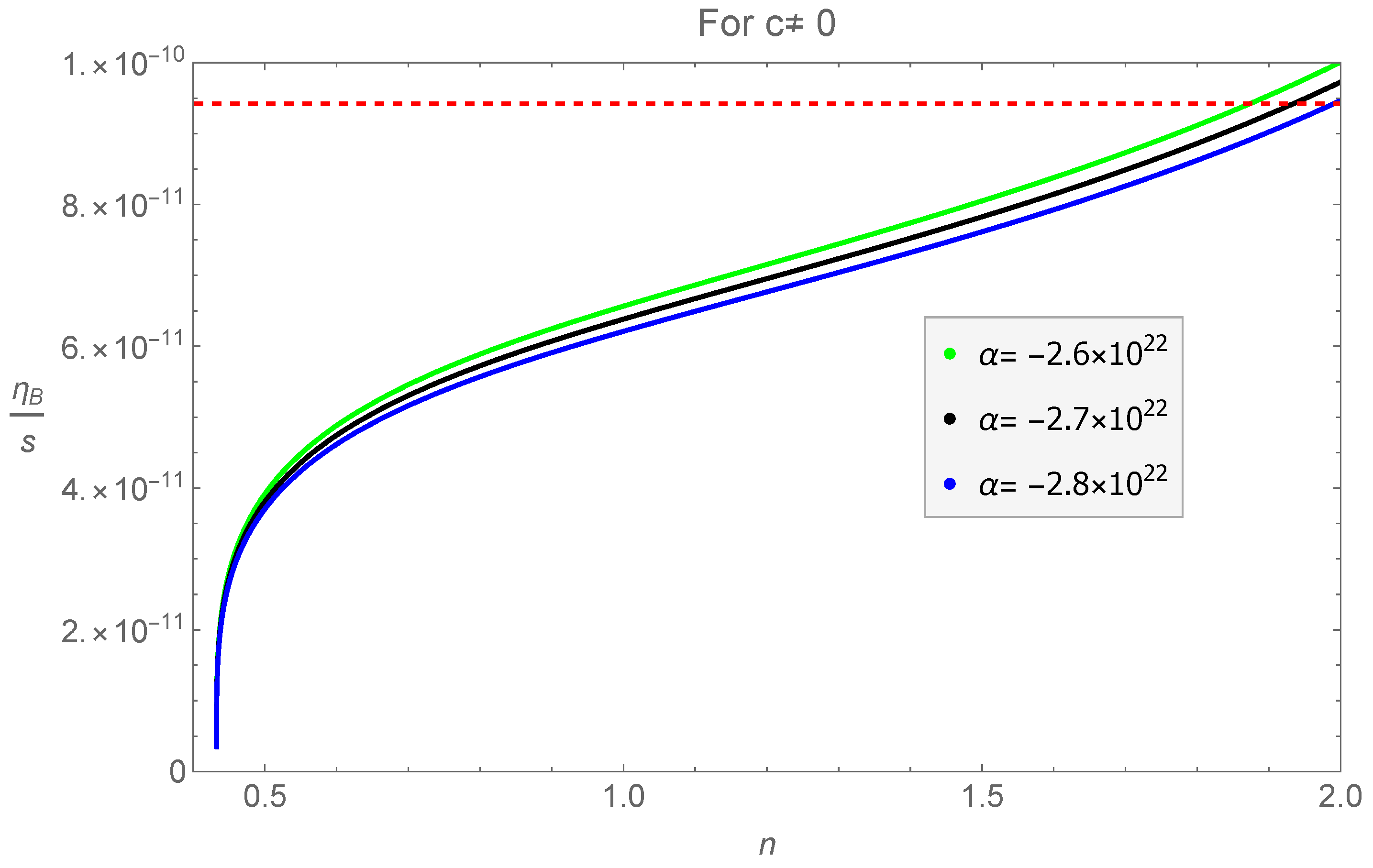Figure 2 represents the graph of $\frac{{\eta }_B}{S}$ against parameter n for different values of $\alpha$, as mentioned in the panel. All other constants chosen are the same as in the previous figure. The graph shows that the inspected ratio remains <$9.42\times {10}^{-11}$ up to when $n<1.86$, resulting in compatibility with the observational data [1,2].

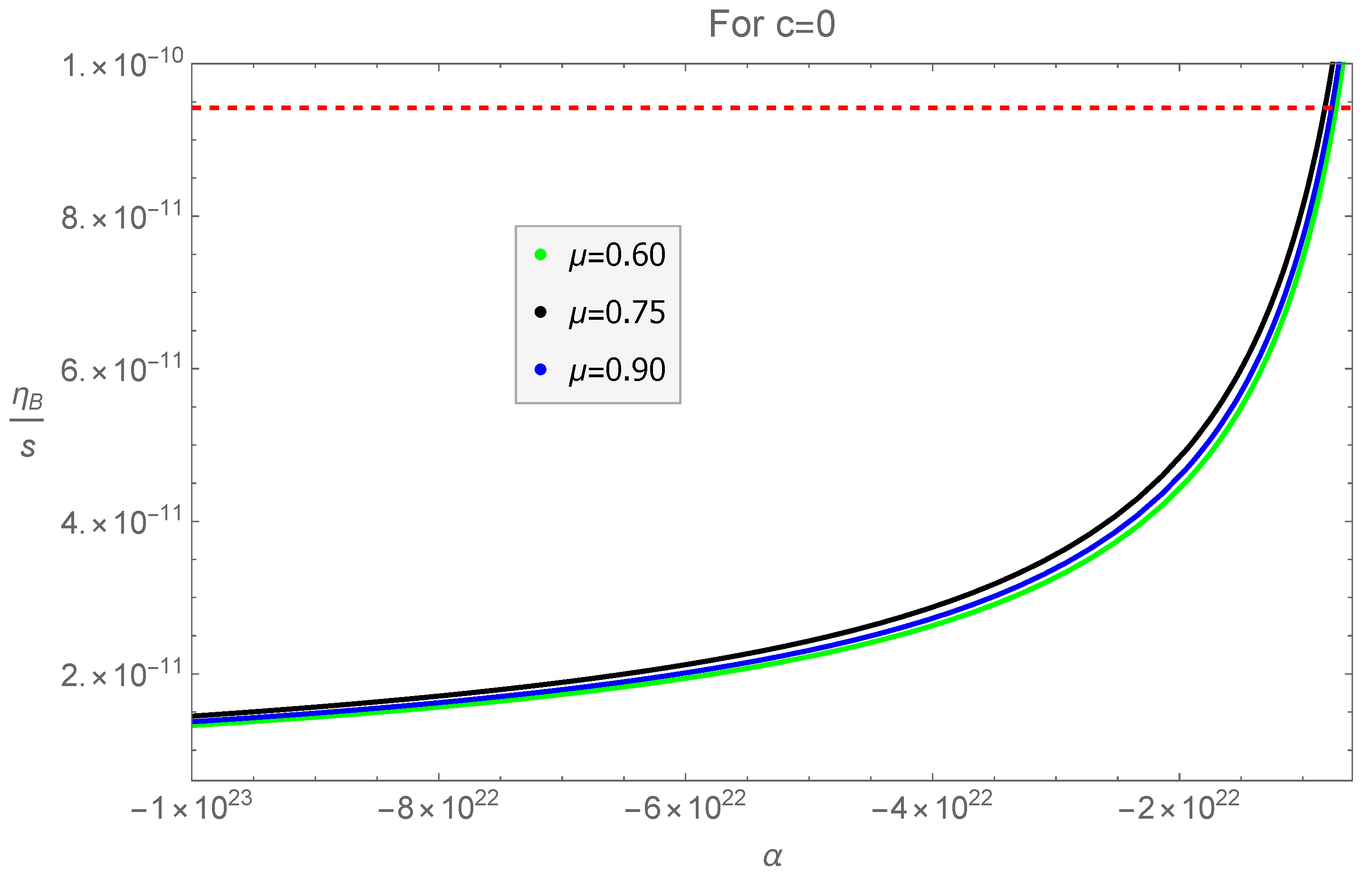
In particular, if we choose the constant $c=0$ in Equation (7), then Equation (23) reduces to

$$\begin{array}{ccc}\hfill \frac{{\eta }_B}{S}{|}_{c=0}& \simeq & \frac{45n(n-3\lambda n+6\mu n-2\mu )g_b}{2{\pi }^2{g}_{*s}{M}_{*}^2{T}_D}\left[\frac{1}{2}\right(\frac{8100n^2}{{\pi }^4{g}_{*s}^2{T}_D^8}{(n-3\lambda n+4\mu )}^2-\frac{120}{{\pi }^2{g}_{*s}{T}_D^4}\hfill \\ \hfill & \times & (54\alpha \lambda n^4-81\alpha {\lambda }^2{n}^4+324\alpha \lambda \mu n^4-324\alpha {\mu }^2{n}^4-108\alpha \mu n^4-9\alpha n^4\hfill \\ \hfill & -& 432\alpha \lambda \mu n^3+864\alpha {\mu }^2{n}^3+144\alpha \mu n^3+324\alpha {\lambda }^2{n}^2-972\alpha \lambda \mu n^2-216\alpha \lambda n^2\hfill \\ \hfill & +& 396\alpha {\mu }^2{n}^2+324\alpha \mu n^2+36\alpha n^2+216\alpha \lambda \mu n-216\alpha {\mu }^{2}n-72\alpha \mu n){)}^{\frac{1}{2}}\hfill \\ \hfill & +& \frac{135\lambda n^2-45n^2-180\mu n}{{\pi }^2{g}_{*s}{T}_D^4}{]}^{-\frac{3}{2}}.\hfill \end{array}$$

(24)

In Figure 3, the ratio $\frac{{\eta }_B}{S}$ has been plotted versus parameter $\alpha$ for varying values of $\mu$, which are ($0.60,0.75,0.90$). In this case, the integration constant c in Equation (7) is chosen to be zero. The other constants are taken to be as $a_0=1$, $g_{{}_b}=1$, $g_{*s}=106$, $\lambda =0.7$, $M_{*}={10}^{12}GeV$, $n=0.5$, and $T_D=2\times {10}^{16}$ GeV. The graph described that $\frac{{\eta }_B}{S}<9.42\times {10}^{-11}$ for $\alpha \lesssim -8\times {10}^{21}$, which is consistent with the current observational data [1,2]. 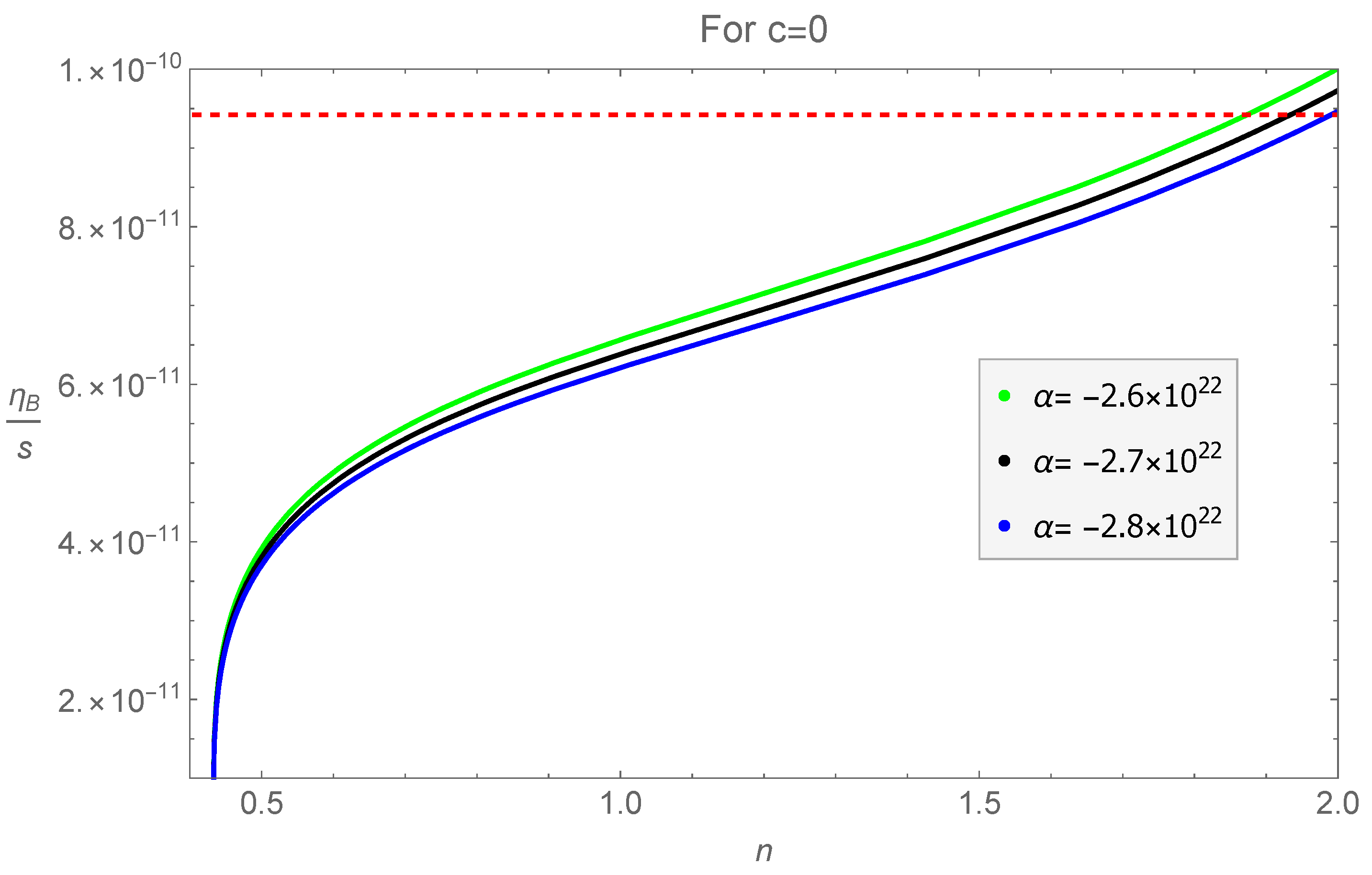Figure 4, shows the graph of ratio $\frac{{\eta }_B}{S}$ against n for various values of parameter $\alpha$. All the parameters are chosen, the same as in the previous plot. The graph describes that $\frac{{\eta }_B}{S}<9.42\times {10}^{-11}$ for $n\lesssim 1.88$, which shows compatibility with the observations [1,2].

5. Model: II

In this section, we are motivated to consider the more generalized and extended functional form of $F\left(\tilde{R}\right)$, which is mathematically given by

$$\begin{array}{c}\hfill F\left(\tilde{R}\right)=\tilde{R}+\alpha {\tilde{R}}^2++\beta {\tilde{R}}^m,\end{array}$$

(25)

where $\alpha$, $\beta$ are non-zero real numbers and $m>2$ is also a real constant. Differentiating Equation (25) with respect to $\tilde{R}$ and substituting the value of $\tilde{R}$ from Equation (15), we obtain

$$\begin{array}{c}\hfill F^{\prime }\left(\tilde{R}\right)=1+\frac{6\alpha n(n-3\lambda n+6\mu n-2\mu )}{t^2}+\frac{\beta m{3}^{m-1}{n}^{m-1}{(n-3\lambda n+6\mu n-2\mu )}^{m-1}}{t^{2(m-1)}}.\end{array}$$

(26)

The above equation leads to

$$\begin{array}{c}\hfill \frac{d{F}^{\prime }\left(\tilde{R}\right)}{dt}=-\frac{12\alpha n(n-3\lambda n+6\mu n-2\mu )}{t^3}-\frac{2(m-1)\beta m{\left[3n(n-3\lambda n+6\mu n-2\mu )\right]}^{m-1}}{t^{2m-3}}.\end{array}$$

(27)

Substituting the values from Equations (13), (15), and (25)–(27) in Equation (7), a simplification yields

$$\begin{array}{ccc}\hfill t^{2m+3n}& -& \frac{90n^2}{{\pi }^2{g}_{*s}{T}_D^4}(3\lambda -1)t^{2m+3n-2}-\frac{90n^2(n-3\lambda n+6\mu n-2\mu )}{{\pi }^2{g}_{*s}{T}_D^4}[3\alpha (n-3\lambda n-2\mu )\hfill \\ \hfill & -& 48\alpha n\mu -12n(1-3\lambda +3\mu )]t^{2m+3n-4}-\frac{30\left(3^m{n}^m\right){(n-3\lambda n+6\mu n-2\mu )}^{m-1}}{{\pi }^2{g}_{*s}{T}_D^4}\hfill \\ \hfill & \times & \left[n-3\lambda n+6\mu n+2\mu m-2\beta mn(1-3\lambda +3\mu )-2\mu \right]t^{3n}+120\mu \beta m\left(3^m{n}^m\right)\hfill \\ \hfill & \times & \frac{{(n-3\lambda n+6\mu n-2\mu )}^{m-1}}{{\pi }^2{g}_{*s}{T}_D^4}{t}^{3n-4}-c{a}_o^{-3}{t}^{2m}=0.\hfill \end{array}$$

(28)

As the above equation is much complicated and impossible to solve, for simplicity, we choose $c=0$; it reduces to

$$\begin{array}{ccc}\hfill t^{2m+4}& -& \frac{90n^2}{{\pi }^2{g}_{*s}{T}_D^4}(3\lambda -1)t^{2m+2}-\frac{90n^2(n-3\lambda n+6\mu n-2\mu )}{{\pi }^2{g}_{*s}{T}_D^4}[3\alpha (n-3\lambda n-2\mu )-48\alpha n\mu \hfill \\ \hfill & -& 12n(1-3\lambda +3\mu )]t^{2m}-\frac{30\left(3^m{n}^m\right){(n-3\lambda n+6\mu n-2\mu )}^{m-1}}{{\pi }^2{g}_{*s}{T}_D^4}[n-3\lambda n+6\mu n+2\mu m\hfill \\ \hfill & -& 2\beta mn(1-3\lambda +3\mu )-2\mu ]t^4+\frac{120m\beta \mu \left(3^m{n}^m\right){(n-3\lambda n+6\mu n-2\mu )}^{m-1}}{{\pi }^2{g}_{*s}{T}_D^4}=0.\hfill \end{array}$$

(29)

When $m=3$, Equation (29) becomes as

$$\begin{array}{ccc}\hfill t^{10}& -& \frac{90n^2}{{\pi }^2{g}_{*s}{T}_D^4}(3\lambda -1)t^8-\frac{90n^2(n-3\lambda n+6\mu n-2\mu )}{{\pi }^2{g}_{*s}{T}_D^4}[3\alpha (n-3\lambda n-2\mu )-48\alpha n\mu \hfill \\ \hfill & -& 12n(1-3\lambda +3\mu )]t^6-\frac{810n^3{(n-3\lambda n+6\mu n-2\mu )}^2}{{\pi }^2{g}_{*s}{T}_D^4}[n-3\lambda n+6\mu n+4\mu -6\beta \hfill \\ \hfill & \times & n(1-3\lambda +3\mu )]t^4+\frac{9720\beta \mu n^3{(n-3\lambda n+6\mu n-2\mu )}^2}{{\pi }^2{g}_{*s}{T}_D^4}=0.\hfill \end{array}$$

(30)

The above mathematical model is still complicated and it is impossible to obtain the general solution. If we assign some particular values to the parameters involved in the coefficients of the model equation, it leads to a constant solution. We assign fixed values to the parameters involved in Equation (30), as $g_{*s}=106$, $\lambda =0.7$, $M_{*}={10}^{12}$ GeV, $n=2$, $T_D=2\times {10}^{16}$ GeV, and $\alpha =5$, by varying the values to the parameter $\mu$ (as mentioned in

Table 1. Baryogenesis for $F\left(\tilde{R}\right)=\tilde{R}+\alpha {\tilde{R}}^2+\beta {\tilde{R}}^m$ when $m=3$.

Sr. No	$\mathit{\mu }$	$\frac{{\mathit{\eta }}_{{}_{\mathit{B}}}}{\mathit{S}}$
1	$-0.90$	$9.453\times {10}^{-23}$
2	$-0.85$	$9.442\times {10}^{-23}$
3	$-0.80$	$9.433\times {10}^{-23}$
4	$-0.75$	$9.426\times {10}^{-23}$
5	$-0.70$	$9.422\times {10}^{-23}$

). For each value of $\mu$, twelve different roots are obtained, among which, eight belongs to a set of complex numbers that cannot be further discussed. Two of them are equal to zero and considered as trivial solutions, while the other two are $\pm 6.33978\times {10}^{-7}$. The solution $6.33978\times {10}^{-7}$ is an extraneous root while $-6.33978\times {10}^{-7}$ is the only solution for the coupling time $t=t_D$, which gives suitable results for the term $\frac{{\eta }_B}{S}$. These values in a point form are mentioned in Table 1. These deduced values provide consistent results with observations of $\frac{{\eta }_B}{S}$. It can be observed from Table 1 that as the value of $\mu$ increases, $\frac{{\eta }_B}{S}$ decreases.

When $m=4$, Equation (29) becomes as

$$\begin{array}{ccc}\hfill t^{12}& -& \frac{90n^2}{{\pi }^2{g}_{*s}{T}_D^4}(3\lambda -1)t^{10}-\frac{90n^2(n-3\lambda n+6\mu n-2\mu )}{{\pi }^2{g}_{*s}{T}_D^4}[3\alpha (n-3\lambda n-2\mu )-48\alpha n\mu \hfill \\ \hfill & -& 12n(1-3\lambda +3\mu )]t^8-\frac{2430n^4{(n-3\lambda n+6\mu n-2\mu )}^3}{{\pi }^2{g}_{*s}{T}_D^4}[n-3\lambda n+6\mu n+6\mu \hfill \\ \hfill & -& 8n\beta (1-3\lambda +3\mu )]t^4+\frac{38880\beta \mu n^4{(n-3\lambda n+6\mu n-2\mu )}^3}{{\pi }^2{g}_{*s}{T}_D^4}=0.\hfill \end{array}$$

(31)

The complications to find the solution of the above mathematical model also exist in this case. To avoid the complication, we assign some particular values to the parameters involved in the coefficients of the above equation, which leads to constant solutions. We assign fixed values to the parameters involved in Equation (31) as $g_{*s}=106$, $\lambda =0.7$, $M_{*}={10}^{12}$ GeV, $n=2$ and $T_D=2\times {10}^{16}$ GeV, $\alpha =5$, and varying values to the parameter $\mu$, as mentioned in

Table 2. Baryogenesis for $F\left(\tilde{R}\right)=\tilde{R}+\alpha {\tilde{R}}^2+\beta {\tilde{R}}^m$ when $m=4$.

S. No	$\mathit{\mu }$	$\frac{{\mathit{\eta }}_{{}_{\mathit{B}}}}{\mathit{S}}$
1	$0.20$	$1.176\times {10}^{-26}$
2	$0.18$	$1.437\times {10}^{-26}$
3	$0.16$	$1.637\times {10}^{-26}$
4	$0.14$	$1.819\times {10}^{-26}$
5	$0.12$	$1.999\times {10}^{-26}$

. For each value of $\mu$, fourteen different solutions for t are obtained, among which ten solutions belong to set of complex numbers that we ignore, as they are impossible to tackle. Two more solutions are equal to zero and considered as trivial solutions, while the other two non-zero real solutions are $\pm 3.31854\times {10}^{-6}$ from which $3.31854\times {10}^{-6}$ is extraneous roots, while $-3.31854\times {10}^{-6}$ is the only solution for which the coupling time $t=t_D$ provides good matchable results with the observational data for $\frac{{\eta }_B}{S}$. It can be observed from Table 2 that as the value of $\mu$ increases, $\frac{{\eta }_B}{S}$ decreases, and remains in the required range.

6. Conclusions and Discussion

The motivation of this research work is to look over the compatibility and consistency of the modified Hořava-Lifshitz theory in the aspect of gravitational baryogenesis with perfect fluid and the FLRW universe. A prerequisite to examining this physical aspect of the universe is to evaluate the coupling time $t=t_D$. For this purpose, we assumed two different models, and the baryon asymmetry is investigated thoroughly. The first model considered is $F\left(\tilde{R}\right)=\tilde{R}+\alpha {\tilde{R}}^2$. This model is analyzed for two different cases. In first case, we examined the ratio $\frac{{\eta }_B}{S}$ when the constant of the integration c in Equation (7) is considered to be non zero. The outcomes in this case are plotted in Figure 1 and Figure 2 for $\frac{{\eta }_B}{S}$ against $\alpha$ and n, respectively. It is found from the figures that the assumed model is efficient and consistent in presenting the observed value of $\frac{{\eta }_B}{S}$. Graphical values exhibit an increase in the baryon to entropy ratio, as the parameter $\alpha$ and n increases. In the second case, the constant c is chosen to be zero in Equation (7), and the baryogenesis phenomenon is investigated. It is found in Figure 3 (the plot of $\frac{{\eta }_B}{S}$ against $\alpha$) and Figure 4 (the graph of $\frac{{\eta }_B}{S}$ versus n) that $\frac{{\eta }_B}{S}$ has an excellent agreement with the observational data [1,2].

The second model considered is more generalized and extended, having a mathematical formalism of $F\left(\tilde{R}\right)=\tilde{R}+\alpha {\tilde{R}}^2+\beta {\tilde{R}}^m$. To evaluate the baryon to entropy ratio for this model, the constant of integration c in Equation (7) is taken to be zero to avoid the complication for the solution of the model equation. This model is analyzed for two different values of m ($m=3$ and $m=4$). The mathematical expression for the coupling time $t=t_D$ was impossible to obtain for both values of m. Therefore, the coupling time, $t_D$, is obtained in a constant form against different values of $\mu$ and a tabular representation of the outcomes is given in spite of the graphical description. For $m=3$, twelve different solutions for the $t=t_D$ were obtained, among which eight were complex and not discussed. The other two solutions were zero, while the remaining two roots were $\pm 0.962195$. From these two values, $t_D=0.962195$ is an extraneous root while $-0.962195$ involves the ratio $\frac{{\eta }_B}{S}$. The baryogenesis phenomenon is calculated for five different values of $\mu$ and results are mentioned in Table 1. The outcomes are that these results are consistent with observational data. It is also observed that as the value of $\mu$ increases, the baryon to entropy ratio decreases.

In the same manner, the baryon to entropy ratio is calculated for $m=4$, which provides fourteen different solutions for $t=t_D$, among which ten were complex and two were equal to zero, which we did not discuss. The other two real solutions were $\pm 3.31854\times {10}^{-6}$ among which the solution, $3.31854\times {10}^{-6}$, behave like extraneous roots. Only the solution $-3.31854\times {10}^{-6}$ was compatible to the observations and hence was considered to analyze the ratio. Taking $t_D=-3.31854\times {10}^{-6}$ into account, five different values of $\mu$ are utilized to find $\frac{{\eta }_{{}_B}}{S}$, which is mentioned in Table 2. It is found that the $\frac{{\eta }_{{}_B}}{S}$ for these values is consistent and remains in the range of observations. Moreover, it is also found that $\frac{{\eta }_{{}_B}}{S}$ decreases as $\mu$ increases.

From all obtained results of the ratio $\frac{{\eta }_{{}_B}}{S}$, it is concluded that modified Hořava-Lifshitz gravity can produce a non-vanishing baryon asymmetry, which is highly compatible with the latest observational bounds for various model parameters.