
On the Bifurcations of a 3D Symmetric Dynamical System

Department of Applied Mathematics, University of Craiova, 200585 Craiova, Romania
Symmetry 2023, 15(4), 923; https://doi.org/10.3390/sym15040923
Submission received: 17 March 2023
/
Revised: 10 April 2023
/
Accepted: 13 April 2023
/
Published: 15 April 2023
(This article belongs to the Special Issue Three-Dimensional Dynamical Systems and Symmetry)
Abstract
:The paper studies the bifurcations that occur in the T-system, a 3D dynamical system symmetric in respect to the Oz axis. Results concerning some local bifurcations (pitchfork and Hopf bifurcation) are presented and our attention is focused on a special bifurcation, when the system has infinitely many equilibrium points. It is shown that, at the bifurcation limit, the phase space is foliated by infinitely many invariant surfaces, each of them containing two equilibrium points (an attractor and a saddle). For values of the bifurcation parameter close to the bifurcation limit, the study of the system’s dynamics is done according to the singular perturbation theory. The dynamics is characterized by mixed mode oscillations (also called fast-slow oscillations or oscillations-relaxations) and a finite number of equilibrium points. The specific features of the bifurcation are highlighted and explained. The influence of the pitchfork and Hopf bifurcations on the fast-slow dynamics is also pointed out.
1. Introduction
The study of bifurcations is a fundamental and challenging topic in the theory of dynamical systems because it highlights the qualitative changes of their behavior over time and gives information on the possible evolution of the systems for various values of the parameters.
The aim of the paper is to study the bifurcations of a 3D symmetric system, namely the T-system that was introduced in [1]. It belongs to the class of the Lorenz system, having the nonlinear term of order two. Despite the simplicity of its equations, it has very rich dynamics.
An important characteristic of the system is its symmetry. It is a well-known fact that symmetries can be used in a systematic way to analyze some general mechanisms of pattern formation, but symmetry methods can also be applied to the study of equilibria and their bifurcations, period-doubling, time-periodic states, homoclinic and heteroclinic orbits and chaos [2,3] (pp. 276–288). Some results concerning the pitchfork and Hopf bifurcations that occur in the T-system are presented in this paper and the influence of the symmetry of the system on its dynamics is highlighted.
But our attention is focused on a special bifurcation, when the system has infinitely many equilibrium points at the bifurcation limit. It is an important topic, both theoretically and through its applications. The coexistence of many attractors usually generates complicated dynamics. Examples of chaotic systems with an infinite number of equilibrium points were proposed and studied in many papers, for example [4,5,6]. Practical applications to secure communications were proposed in [7] and the extreme multi-stability (i.e., the coexistence of infinitely many attractors) was found to occur in memristor-based systems [8,9].
We show that, for the T-system at the bifurcation limit, the phase space is foliated by infinitely many invariant surfaces, each of them containing two equilibrium points: an attractor and a saddle.
The study of the dynamics of the system for values of the bifurcation parameter that are close to the bifurcation limit is made in the frame of the singular perturbation theory. It is shown that the system exhibits fast-slow dynamics. The periodic motions consist of a long time-interval of a quasi-steady state followed by a short time-interval of rapid variations. They are called relaxation-oscillations [10]. The main tool in the study of such systems is the geometric singular perturbation theory introduced by Fenichel N. in [11]. Fenichel’s theorem is based on the assumption that the critical manifold is normally hyperbolic. When some points of the critical manifold are not normally hyperbolic some more advanced tools, such as the blow-up method [12] or the entry-exit function method [13,14] may be applied.
For the T-system it is shown that the critical set, which is symmetric with respect to the z-axis, is formed by two intersecting lines. One of them is made up only of points that are not normally hyperbolic. In this situation, Fenichel’s theory is applied with caution when possible and the mechanism of relaxation-oscillation is explained using exchange-lemmas arguments [15].
Some aspects of the dynamics of the singularly perturbed T-system when the pitchfork and the Hopf bifurcation occur are also presented. It is observed that the Hopf bifurcation does not essentially influence the fast-slow dynamics of the system, but the pitchfork bifurcation is somehow dominant compared with the fast-slow dynamics.
The paper is organized as follows: in Section 2 the T-system is introduced; Section 3 is devoted to the study of the equilibrium points, their stability, and bifurcations; in Section 4 the dynamics of the singularly perturbed T-system are studied, while some aspects of the dynamics of the singularly perturbed T-system in the presence of Hopf and pitchfork bifurcations are highlighted in Section 5; conclusions are summarized in Section 6.
2. The T-System, General Properties
The T-system is a 3D autonomous system depending on three parameters, , , , defined by
Some of its properties have been studied in many papers: stability analysis [16], the existence of heteroclinic orbits [17,18], and bifurcations with delayed feedback [19]. The fractional-order T-system was derived and studied in [20].
For the system is linear and has no particular interest from a dynamic point of view. In what follows we consider . Using the transformation
the system (1) can be written as
where and . The system (2) has the advantage of having only two parameters: the study of the bifurcations using the plane of parameters becomes easier.
Depending on the values of the two parameters and , a rich dynamics of the system (2) occurs.
Proposition 1.
The involutive diffeomorphism , is a symmetry of the system (2).
Proof of Proposition 1.
We denote and simple computation shows that . □
The existence of symmetry has important consequences on the dynamics of the system:
- If is an equilibrium point of the system, then is also an equilibrium point of the system and they have both the same type of stability. The two points are called -conjugated [3] (p. 279). Consequently, twin bifurcations of the -conjugated equilibrium points occur.
- The set is the fixed-point subspace of (2). It is invariant under the flow of the system, so the orbits entirely lie in , or entirely lie outside of .
The symmetry group is and one can use some specific techniques to study the bifurcations [3] (pp. 276–288).
The space is decomposed into a direct sum, , where and .
3. Equilibrium Points, Their Stability and Bifurcations
Proposition 2.
(a) For and the system (2) has a unique equilibrium point which is an attractor. (b) For and the system (2) has a unique equilibrium point which is non-hyperbolic, with and . (c) For and the system (2) has three equilibrium points: which is a saddle node with and and the -conjugated equilibrium points. , which are stable foci if or saddle foci with and if . (d) For and the system (2) has infinitely many non-hyperbolic equilibrium points.
Proof of Proposition 2.
Solving the system one obtains the unique solution for , an infinite number of solutions for and the solutions , for .
The characteristic polynomial of is .
- (a)
- For all eigenvalues of the Jacobian matrix have negative real parts. So is an attractor.
- (b)
- For the eigenvalues are . So is not hyperbolic and , .
- (c)
- For there are three equilibrium points.
The Jacobian matrix of the equilibrium point has three real eigenvalues: , and . It is a saddle point with and .
The characteristic polynomials of and coincide, their common form is .
Because and , it results that the equation has at least one solution . But the equation has not positive solutions, because for all , so for all .
The equation has not two negative solutions (in this case the third one is positive, contradiction with the previous observation). Finally, it results that the equation has a strictly negative solution and two complex conjugated solutions.
Using the Routh-Hurwitz criterion, one obtains that the equation has three solutions with strictly negative real parts if and only if . Because , it reads .
It results that and if and only if .
It means that and are stable foci if and only if .
If , there is a strictly negative eigenvalue and two eigenvalues with strictly positive real parts. It means that and are saddle foci with and .
- (d)
- For the characteristic polynomial of is . Because it results that is not hyperbolic. □
3.1. The Pitchfork Bifurcation
The bifurcating equilibrium is of the fixed type, i.e., it is situated on the fixed-point subspace of the system (2).
For , is attractor, becomes non-hyperbolic for and two branches of -conjugated equilibrium points appear for . This is a typical configuration for the pitchfork bifurcation.
Proposition 3.
The system (2) undergoes a pitchfork bifurcation of in .
Proof of Proposition 3.
The system (2) has two important properties:
- (a)
- it is -symmetric, at it has a fixed equilibrium with the simple eigenvalue and the corresponding eigenvector .
- (b)
- the eigenvector belongs to the .
In this case, the hypothesis of Theorem 7.7 [3] (p. 281) is fulfilled and it results that the system (2) has a one-dimensional -invariant center manifold and , for all sufficiently small . More of this, the restriction of the system to is locally topologically equivalent near the origin to the following normal form: . It means that a pitchfork bifurcation of occurs in . □
From Proposition 2(c) it results that are stable foci for . At the same time, is a saddle node with and .
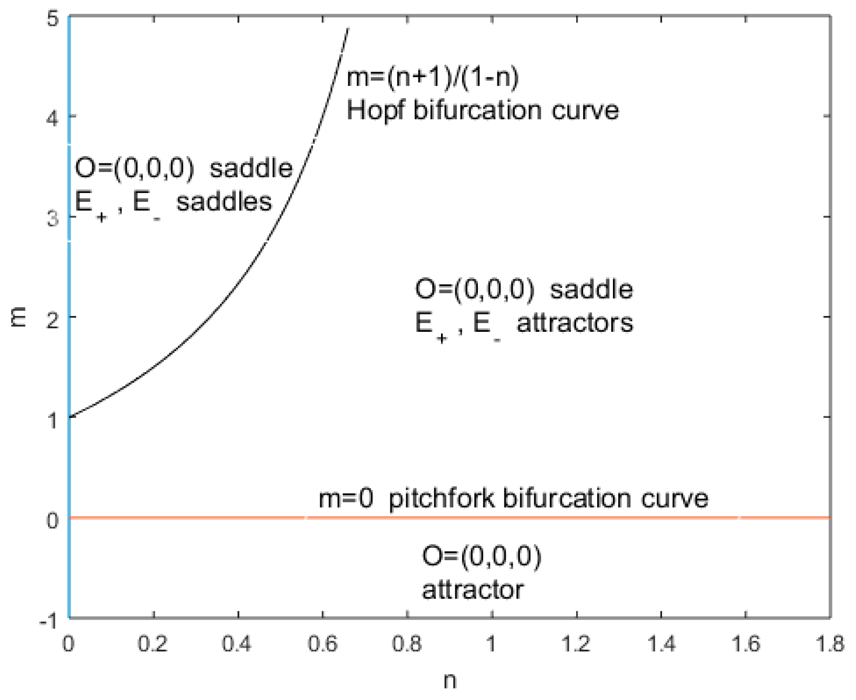
In Figure 1 the pitchfork bifurcation curve, , is presented in the parameters’ plane.
For the system (2) has a unique equilibrium point, , which is attractor. For the equilibrium point is not hyperbolic. For the equilibrium point is a saddle and two branches of -conjugated equilibrium points appear. The -conjugated equilibrium points and are attractors if and only if .
The physical interpretation of these results is that the two branches of S-conjugated equilibrium points appear when , corresponding to the cancelation of the linear term in the second equation of the system (2).
It is interesting to mention that the existence of the symmetry is essential in demonstrating the occurrence of the pitchfork bifurcation, because the system (2) does not satisfy the assumptions of other classical theorems, such as Sotomayor’s theorem [21] (p. 338).
3.2. The Hopf Bifurcation of
The Hopf bifurcation of in the system (2) was studied in [16]. The main result is the following.
Proposition 4.
For and , the system (2) undergoes non-degenerate twin Hopf bifurcations in and if and .
In order to study the twin Hopf bifurcations that occur in and one follows the classical algorithm [3] (p. 112): consider that the eigenvalues of the system (2) are functions of having the form and check the conditions of Hopf’s Theorem.
The condition gives . For we have .
More of this, .
The first Lyapunov coefficient is , (see [16] for details).
For the -conjugated equilibrium points and are saddle foci and they are not hyperbolic for . For the two equilibrium points are attractors and two -conjugated unstable limit cycles are formed near them. In [22] is shown that the -conjugated unstable limit cycles generated through the Hopf bifurcation for have a one-dimensional stable manifold and a one-dimensional unstable manifold. The coexistence of unstable limit cycles with a chaotic attractor, exemplified using the system (2), was considered in [22] an important dynamical aspect that was not pointed out before.
4. The Singular Bifurcation
A singular bifurcation occurs in : for the system (2) has infinitely many equilibrium points and for the system (2) has one or three equilibrium points (if , respectively ).
The main physical interpretation is that the existence of infinitely many equilibrium points (when n = 0) is strongly related to the absence of the linear terms in the third equation of the system (2).
In the following, we will study the case and we will consider as a perturbation parameter. The bifurcation will be analyzed according to the singular perturbation theory.
4.1. The Dynamics of the Unperturbed System
The unperturbed system, obtained from (2) for , is
Proposition 2(d) already stated that the fixed-point subspace is formed by equilibrium points.
Proposition 5.
(a) The unperturbed system (3) has infinitely many invariant surfaces . (b) For , the equilibrium point is non-hyperbolic, with and . (c) For , each invariant surface contains two non-hyperbolic equilibria and . is asymptotically stable and is a saddle point for the system (3) restricted to .
Proof of Proposition 5.
(a) Let consider . Simple computation shows that . It means that is a first integral of (3) and the surfaces are invariant surfaces for (3) for all . (b) contains the unique equilibrium having the characteristic polynomial . The eigenvalues are and . (c) The equilibrium points of (3) situated on must fulfill the conditions . They are and .
The characteristic polynomial of is . The eigenvalues of are and , which have a negative real part for all .
The characteristic polynomial of is . The eigenvalues of are , and , for all . □
The system (3) is dissipative because , where . Hence the orbits of all points , with , are attracted by , excepting those starting from the stable manifold of .
4.2. Fast-Slow Oscillations in the Perturbed System
For the system (2) is a fast-slow system with two fast variables and one slow variable, not written in the standard form for the moment. The standard form is obtained using the transformation
The system (2) becomes
4.2.1. The Dynamics of the Fast Subsystem
The fast subsystem is obtained by considering in (4):
The critical set is formed by two lines that intersect in :
The fast subsystem describes the evolution of the fast variables and far from the critical set .
The third equation of (5) shows that for all , so may be considered a parameter in the system formed by the first two equations. System (5) is equivalent to the system
We consider and the solutions of the characteristic equation
For one has and the orbit of is given by , where
For one has and the orbit of is given by , where
Proposition 6.
Let us consider the fast subsystem (5).
- (a)
- The plane is invariant with respect to the flow of (5), for all .
- (b)
- For , is the global attractor for the system (5) restricted to the plane .
- (c)
- For , is a saddle point for the system (5) restricted to the plane . The stable manifold of is and the unstable manifold is where are the solutions of the equation . All orbits starting from the plane are unbounded, excepting those starting from the stable manifold of .
- (d)
- For the line is formed by non-hyperbolic equilibrium points and it is the global attractor of the system (5) restricted to the plane .
Proof of Proposition 6.
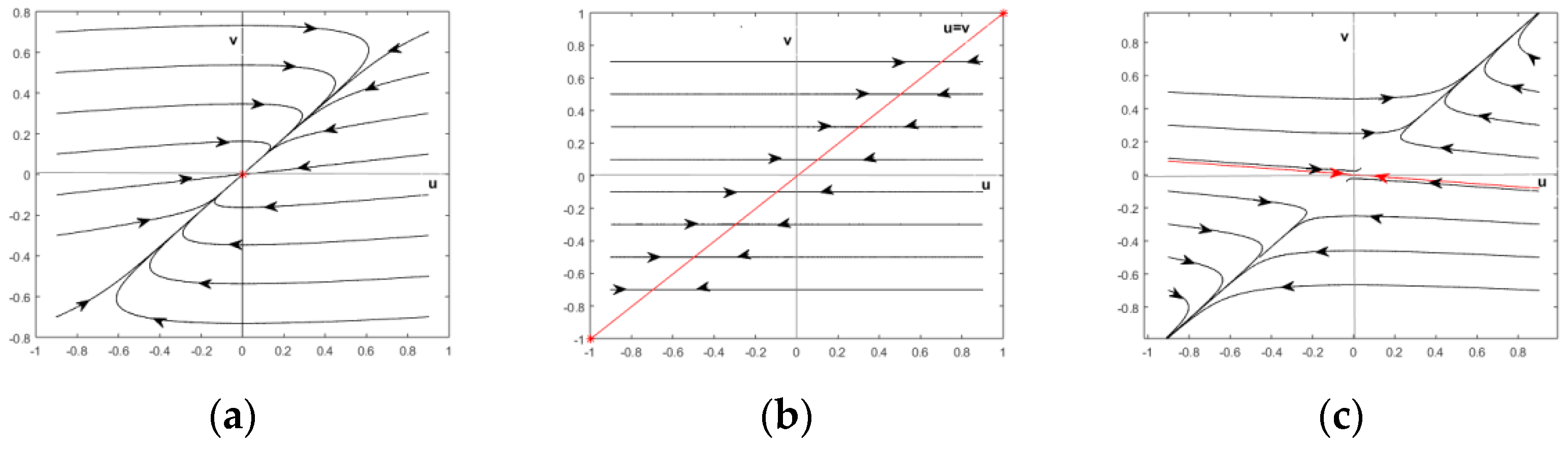
(a) It results immediately from the equation . (b) For and , the characteristic Equation (7) becomes . It has two complex conjugated with negative real parts for , if then and for the equation has two negative solutions. In all cases, it results from (8) and (9) that for all . (c) For and the characteristic Equation (7) becomes . It has a negative solution and a positive one , which shows that is a saddle. The stable and unstable manifolds are obtained from the analytical expression of and . They correspond to , respectively . They are : , respectively : . From (8) it results that if and if i.e., . (d) For , which means , the characteristic equation has the solutions , so . □
In Figure 2 are presented some orbits of the fast subsystem (5) corresponding to , restricted to the plane . In Figure 2a, obtained for , is observed that all orbits are attracted by , corresponding to . Figure 2b, obtained for , shows that the line is formed by stable equilibria that are not asymptotically stable and it represents the global attractor of the system (5) restricted to the plane . Figure 2c, obtained for , shows some unbounded orbits, but also the stable manifold of (the red curve). The unbounded orbits are approaching the unstable manifold of , which is given explicitly in this case by .
The set is formed by fast-slow regular points (which are also normally hyperbolic points) and the set is formed by fast-slow singular points (which are not normally hyperbolic points (see [23] (p. 58) for definitions). In their intersection, , which is a singular point, the stability of the regular points changes from attractor (if ) to saddle (if ).
4.2.2. The Dynamics of the Slow Subsystem
The slow subsystem of (2), corresponding to the slow time , is
where .
The slow subsystem, also called “the reduced problem”, is a differential-algebraic system that describes the dynamics of the slow variable “z” on the critical set . Initial conditions must satisfy the constraints and . Obviously, the third equation of (8) gives .
, the first branch of , is an invariant set of the slow subsystem (10). is the global attractor for the slow subsystem restricted to because the orbit of is .
, the second branch of , is not an invariant set of the slow subsystem because for . It does not play a special role in the formation of fast-slow oscillations.
4.2.3. The Mechanism of the Fast-Slow Oscillations
The orbits of the (full) fast-slow system (4), which is equivalent to the system (2), consist of a slow variation of the (slow) variable and fast motions of the (fast) variables , followed by long periods in which they remain close to 0. They are formed by an alternating sequence of fast and slow orbits, known as fast-slow oscillations or oscillation-relaxation phenomenon. It is expected that near the critical set the orbits of the full system may be approximated by the orbits of the slow system and, sufficiently far from , the slow motion of the variable is irrelevant and the orbits follow the trajectories of the fast subsystem.
The first segment of an orbit starting from , with is a fast orbit, approaching the line , because the fast subsystem is dominant.
This is an immediate consequence of Proposition 6. If , it was proved (Proposition 6(b)) that .
The second segment of the orbit is a slow orbit, because it starts near the critical set, where the slow sub-system is dominant. In this case, slowly decreases.
The orbit continues to be attracted by as long as and repelled by when , because the critical set loses the normal hyperbolicity in the “turning point” and passes from attractive to repulsive dynamics.
But the orbit does not leave as soon as the critical set becomes unstable at and it stays near until its repulsion balances the attraction that occurred before .
Indeed, if , one has in the slow system. Because from that moment one has , the orbit becomes close to the unstable part of and from now on it is reppeled by . It leaves following the unstable manifolds of the saddle points , which are (Proposition 6(c)). For one has and is increasing (because ). remains negative as long as (i.e., the attraction accumulated when is still dominant) and becomes positive when (the repulsion accumulated when is dominant). Basically, the moment when , i.e., the attraction that was exerted by as long as is compensated by the rejection of when , is the starting moment of the fast motion.
Because is increasing, it will become larger than and the procedure is repeated: the orbit is attracted by , enters the half space , is repelled by , crosses the plane and so on.
This phenomenon, when the orbits of a fast-slow system stay near a curve of equilibrium points of the fast subsystem and do not leave it immediately after entering the repelling zone, has been called “bifurcation delay” in [24] or “delay of stability” in [15].
For orbits starting from , with , the action of the fast sub-system is dominant. The first part of the orbit is a fast one (see the arguments previously presented), the orbit enters the half space and the procedure is repeated.
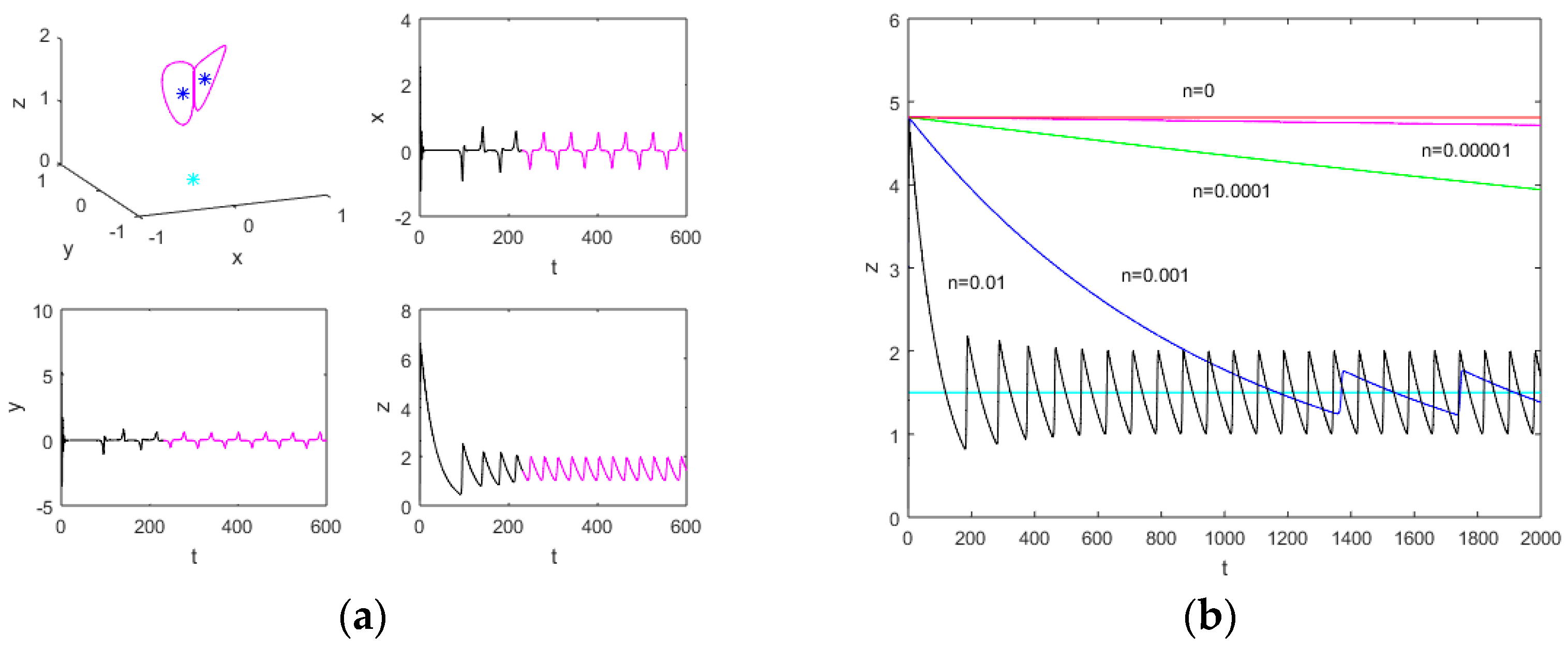
Figure 3a presents the orbit of in the system (2), corresponding to and . One can observe the increase of from to and the important effect of the fast-slow dynamics from the first oscillation. It can also be observed that, after the first oscillation, one has (which confirms the theoretical results).
4.3. From Stable Equilibria to Fast Slow Oscillations
For system (2) has infinitely many non-hyperbolic equilibrium points, , which are stable (but not asymptotically stable) for and unstable for . The orbits starting from , with , are included in and they are attracted by , excepting those starting from the stable manifold of .
For , system (2) has three equilibrium points: and . Typical orbits of (2) exhibit fast-slow oscillations for all .
A visible gap occurs between the dynamics of the system (2) for n > 0, respectively n = 0.
What happens when ?
For , the orbits starting from the surface remain close to it for some time, because . They approach the axis near , which confirms the dynamical dominance of the fast sub-system.
Once the orbit gets close to the axis, the action of the slow sub-system becomes dominant (as presented in the previous paragraph).
Because is very small (), the vertical downward motion is slow. It is slower for smaller values of .
It means that, for a transient time, the orbit will remain in the vicinity of . After this, it will slowly go down, it will descend below the plane and from this moment it will exhibit fast-slow oscillations.
The variation of along the orbit of the system (2) starting from is presented in Figure 3b. The parameter is fixed and various values of are considered: (red curve), (magenta curve), (green curve), (blue curve), and (black curve).
It is interesting to point out that the amplitudes of the oscillations decrease when decreases. At the same time, their periods increase.
In conclusion, there is a qualitative difference between the dynamics of the unperturbed system and the dynamics of the perturbed one. But, for small values of the bifurcation parameter , the dynamics of the perturbed system “mimics” the dynamics of the unperturbed one for a transient time (which is longer when is smaller).
5. Singularly Perturbed System and Local Bifurcations
In the plane of the parameters the pitchfork bifurcation curve and the Hopf bifurcation curve intersect the singular bifurcation curve in respectively (see Figure 1).
An interesting and natural question concerns the interaction between the fast-slow dynamics of the system and the one imposed by the (local) pitchfork and twin Hopf bifurcations i.e., when , respectively .
5.1. Singularly Perturbed System and Pitchfork Bifurcation
As shown in Section 3, two S-conjugated asymptotically stable equilibrium points are formed through a pitchfork bifurcation for . Their basins of attraction are S-conjugated.
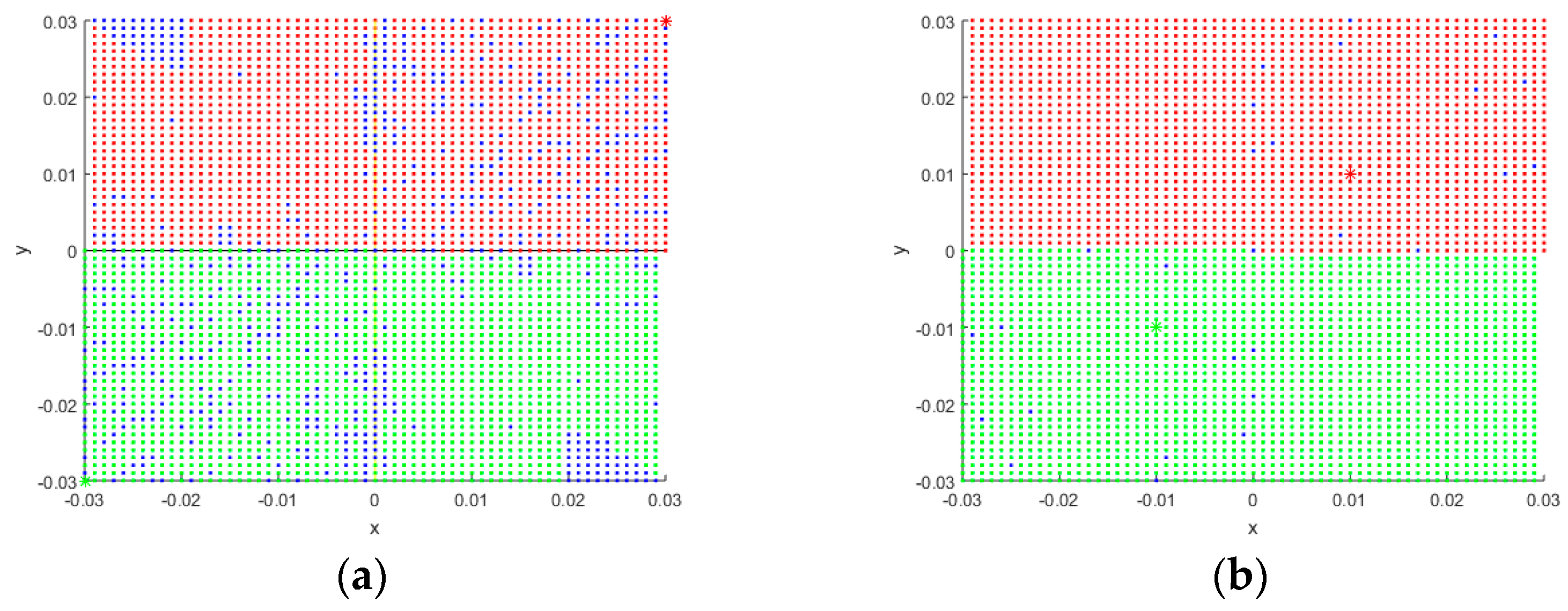
In Figure 4 we synthetized the dynamics of the system (2) near the Oz axis for n = 0.01 and m = 0.09 (Figure 4a) and m = 0.01 (Figure 4b). In the plane (it is the plane where the twin equilibrium points are situated and it is also the plane crossed by the fast-slow oscillations), a grid of 3600 points in the square was considered and the orbit of each point was analyzed in the time interval [2000, 3000]. The orbits of the red points converge to , those of the green points converge to and the orbits of the blue points are oscillating. It can be observed that the dynamics generated by the pitchfork bifurcation is dominating for m = 0.09 and this fact is more effective for m = 0.01.
For and the twin equilibrium points and the saddle point are very close. The singular perturbation is dominant at the beginning of the motion, when the fast subsystem is acting (the orbit approaches the Oz axis) and the slow subsystem causes the orbit to descend along the Oz axis to . When the orbit is rejected by the Oz axis and some oscillations (in the fast-slow scenario) are observed. When the orbit enters the basins of attraction of or , that are very close to Oz axis, it is attracted by one of the asymptotically stable equilibrium points. The variables and , corresponding to the fast variables and in system (4) do not exhibit fast-slow dynamics.
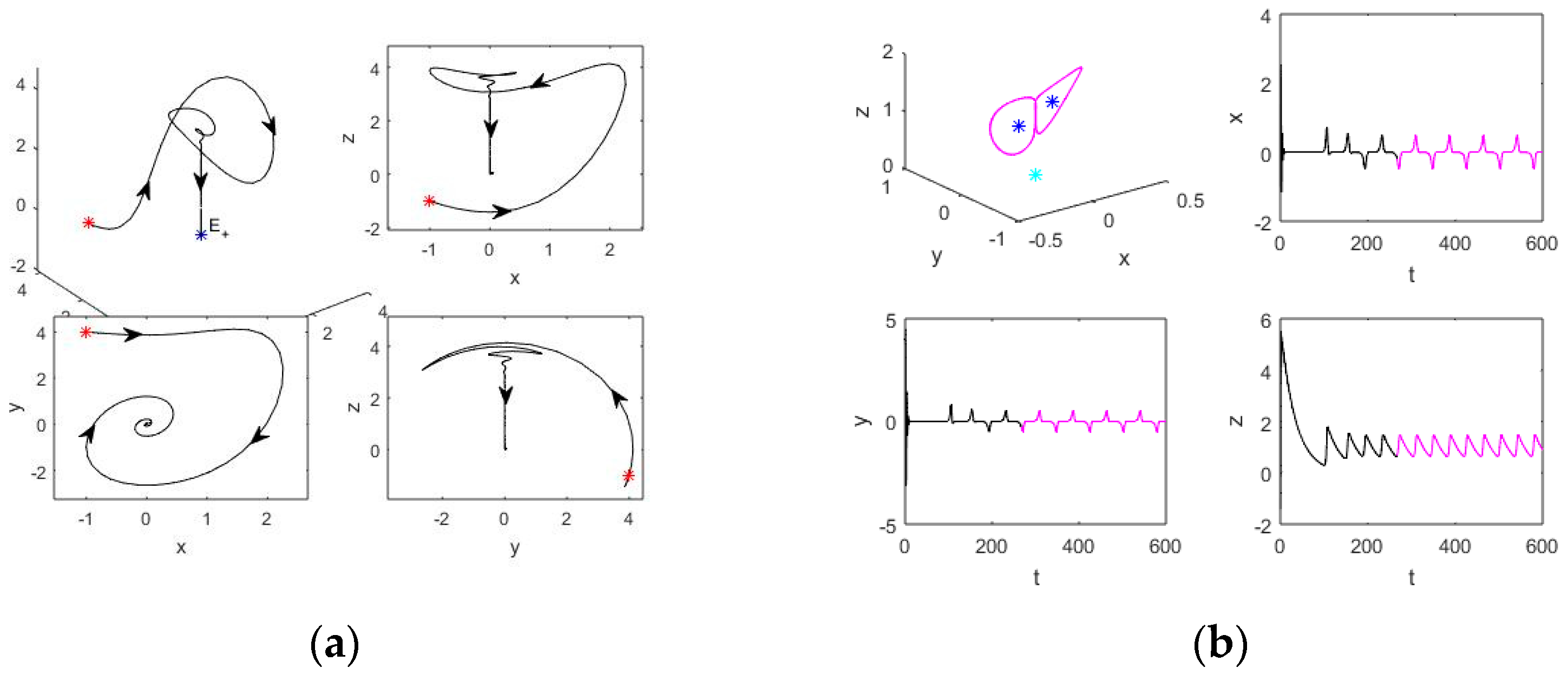
In Figure 5a is presented a typical orbit in system (2) for n = 0.03 and m = 0.05 (after the pitchfork bifurcation: the orbit is attracted by the asymptotically stable equilibrium point ).
Taking into account the numerical simulations, we can state that, when and , the existence of the twin attractive equilibrium points is decisive for the dynamics of the system.
5.2. Singularly Perturbed System and Hopf bifurcation.
As shown in Section 3, S-symmetric unstable cycles are formed through Hopf bifurcations of for when .
For , the estimation of is .
Numerical simulations highlight the existence of a stable periodic orbit (relaxation-oscillation) before and after the Hopf bifurcation, due to the fast-slow characteristics of (2). The formation of the twin unstable cycles for does not essentially influence the fast-slow dynamics because they attract only the points situated on their 1D stable manifold.
In Figure 4b is presented the orbit of in system (2) for and . In the 3D representation the blue points are the equilibrium points , which are saddles; the cyan one is the equilibrium point , which is also a saddle. In the representation of each component of the orbit, the black part represents the evolution until the stabilization near the fast-slow periodic orbit and the magenta part describes the evolution after stabilization.
For and the dynamics is quite complicated: some orbits are attracted by the stable equilibrium points , an unstable limit cycle is formed through the Hopf bifurcation and a double scroll attractor originating from the fast-slow dynamics exists. The double scroll attractor is a periodic orbit for small values of n, but for larger values of it is a strange attractor, similar to the one observed in the Lorenz system. The strange attractor is formed before the Hopf bifurcation occurs (for ), see [16] for details.
6. Conclusions
Despite its simple equations, the T-system exhibits interesting dynamics. In the form (2), a main advantage in studying it is that it depends only on two parameters ( and ), which makes the study of the bifurcations easier. Another advantage is that the fast and the slow subsystems are integrable and the precise solution of the two subsystems can be obtained.
Classical arguments and methods were used in order to obtain results about the pitchfork and Hopf bifurcations and special attention was given to the study of a special bifurcation (we call it “singular bifurcation”) which occurs if : for , the system has a finite number of equilibrium points (a single one for , three equilibrium points for , respectively) and it has infinitely many equilibria for .
For the system was studied according to the singular perturbation theory. In this case, a fast-slow dynamics was observed and analyzed.
The specific features of the bifurcation were highlighted and explained. It was shown that the perturbed system mimics the dynamics of the unperturbed one for a finite time period, if is small enough.
Because the singular bifurcation curve intersects the pitchfork bifurcation curve in and the Hopf bifurcation curve in , the influence of the pitchfork and Hopf bifurcations on the fast-slow dynamics was also pointed out. It was observed that, for , the symmetric equilibrium points generated by the pitchfork bifurcation are very close to the critical set of the system and their attraction dominates the fast-slow dynamics. For fast-slow stable periodic orbits are observed before and after the Hopf bifurcation, so the occurrence of the Hopf bifurcation does not essentially change the dynamics of the systems and it has only local effects.
Funding
This research received no external funding.
Acknowledgments
The present work has been conducted in the context of the GRANT Dynamics H2020-MSCA-RISE funded by The European Union under the contract 777911/2017.
Conflicts of Interest
The author declares no conflict of interest.
References
- Tigan, G. Analysis of a dynamical system derived from the Lorenz system. Sci. Bull. Politehnica Univ. Timisoara Tomul. 2005, 50, 61–72. [Google Scholar]
- Golubitsky, M.; Stewart, I. Progress in mathematics from equilibrium to chaos in phase space and physical space. In The Symmetry Perspective; Birkhäuser Verlag: Basel, Switzerland, 2002; Volume 200. [Google Scholar]
- Kusnetsov, Y.A. Elements of Applied Bifurcation Theory; Springer: New York, NY, USA, 1998. [Google Scholar]
- Jafary, S.; Sprott, J.C. Simple chaotic flows with a line equilibrium. Chaos Solitons Fractals 2013, 57, 79–84. [Google Scholar] [CrossRef]
- Pham, V.T.; Jafari, S.; Volos, C.; Kapitaniak, T. A gallery of chaotic systems with an infinite number of equilibrium points. Chaos Solitons Fractals 2016, 93, 58–63. [Google Scholar] [CrossRef]
- Marwan, M.; Tuwankotta, J.M. Infinitely many equilibria and some codimension one bifurcations in a subsystem of a two-preys one predator dynamical system. J. Phys. Conf. Ser. 2019, 1245, 012063. [Google Scholar] [CrossRef]
- Moysis, L.; Volos, C.; Pham, V.T.; Goudos, S.; Stouboulos, I.; Gupta, M.K.; Mishra, V.K. Analysis of a chaotic system with line equilibrium and its application to secure communications using a descriptor observer. Technologies 2019, 7, 76. [Google Scholar] [CrossRef] [Green Version]
- Bao, H.; Ding, R.; Hua, M.; Wu, H.; Chen, B. Initial-Condition Effects on a Two-Memristor-Based Jerk System. Mathematics 2022, 10, 411. [Google Scholar] [CrossRef]
- Chen, B.; Cheng, X.; Bao, H.; Chen, M.; Xu, Q. Extreme Multistability and Its Incremental Integral Reconstruction in a Non-Autonomous Memcapacitive Oscillator. Mathematics 2022, 10, 754. [Google Scholar] [CrossRef]
- Krupa, M.; Szmolyan, P. Relaxation oscillation and canard explosion. J. Differ. Equ. 2001, 174, 312–368. [Google Scholar] [CrossRef] [Green Version]
- Fenichel, N. Geometric Singular Perturbations Theory for Ordinary Differential Equations. J. Differ. Equ. 1979, 31, 53–98. [Google Scholar] [CrossRef] [Green Version]
- Alvarez, M.J.; Ferragut, A.; Jarque, X. A survey on the blow up technique. Int. J. Bifurc. Chaos 2011, 21, 3103–3118. [Google Scholar] [CrossRef] [Green Version]
- De Maesschalck, P.; Schecter, S. The entry-exit function and geometric singular perturbation theory. J. Differ. Equ. 2016, 260, 6697–6715. [Google Scholar] [CrossRef]
- Hsu, T.H.; Ruan, S. Relaxation oscillations and the entry-exit functions in multidimensional slow-fast systems. SIAM J. Math. Anal. 2021, 53, 3717–3758. [Google Scholar] [CrossRef]
- Liu, W. Exchange Lemmas for singular perturbation problems with certains turning points. J. Differ. Equ. 2000, 167, 134–180. [Google Scholar] [CrossRef] [Green Version]
- Van Groder, R.A.; Roy Choudhury, S. Analytical Hopf bifurcation and stability analysis of T-system. Commun. Theor. Phys. 2011, 55, 609–616. [Google Scholar] [CrossRef]
- Tigan, G.; Constantinescu, D. Heteroclinic orbits in T and Lu systems. Chaos Solitons Fractals 2009, 42, 20–23. [Google Scholar] [CrossRef]
- Algaba, A.; Fernandez-Sanchez, F.; Merino, M.; Rodríguez-Luis, A. On Shilnikov analysis on homoclinic and heteroclinic orbits of the T-system. J. Comput. Nonlinear Dyn. 2013, 8, 027001. [Google Scholar] [CrossRef]
- Zhang, R. Bifurcation analysis for T-system with delayed feedback and its applications to control of chaos. Nonlinear Dyn. 2013, 72, 629–641. [Google Scholar] [CrossRef]
- Liu, X.; Hong, L.; Yang, L. Fractional-order complex T-system: Bifurcations, chaos control and synchronization. Nonlinear Dyn. 2014, 75, 589–602. [Google Scholar] [CrossRef]
- Perko, L. Differential Equations and Dynamical Systems; Springer: New York, NY, USA, 2001. [Google Scholar]
- Constantinescu, D.; Tigan, G.; Zhang, X. Coexistence of Chaotic Attractor and Unstable Limit Cycles in a 3D Dynamical System. Available online: https://open-research-europe.ec.europa.eu/articles/1-50/v1 (accessed on 17 May 2021).
- Kuehen, C. Multiple Time Scale Dynamics; Springer International Publishing: Cham, Switzerland, 2015. [Google Scholar]
- Benoit, E. Linear Dynamic Bifurcation with Noise. In Proceedings of the Dynamic Bifurcations (Luminy, 1990), Lecture Notes in Math. 1493, Luminy, France, 5–10 March 1990; Springer: New York, NY, USA, 1991; pp. 131–150. [Google Scholar]
Figure 1.
The pitchfork and Hopf bifurcation curves in the parameters’ plane.

Figure 2.
Orbits of the fast subsystem (5) restricted to the plane . (a) and ; (b) ; (c) , .

Figure 3.
(a) The orbit of (0.2, 5, 0.2) in system (2) for n = 0.03 and m = 1.5 (fast-slow oscillations); (b) time series from the orbit of (0.2, 3, 0.1) in system (2) for m = 1.5 and n = 0 (red curve), n = 0.00001 (magenta curve), n = 0.0001 (green curve), n = 0.001 (blue curve) and n = 0.01 (black curve).

Figure 4.
The synthesis of the dynamical behavior of some points situated in the plane , for and (a) , (b) . The red points are in the basin of attraction of , the green points are in the basin of attraction of and the orbits of the blue points are ocsillating.
Figure 4.
The synthesis of the dynamical behavior of some points situated in the plane , for and (a) , (b) . The red points are in the basin of attraction of , the green points are in the basin of attraction of and the orbits of the blue points are ocsillating.

Figure 5.
The orbit of (−1, 4, −1) in system (2) for n = 0.03 and (a) m = 0.05 (after pitchfork bifurcation); (b) m = 1.06185 (before Hopf bifurcation).
Figure 5.
The orbit of (−1, 4, −1) in system (2) for n = 0.03 and (a) m = 0.05 (after pitchfork bifurcation); (b) m = 1.06185 (before Hopf bifurcation).

Disclaimer/Publisher’s Note: The statements, opinions and data contained in all publications are solely those of the individual author(s) and contributor(s) and not of MDPI and/or the editor(s). MDPI and/or the editor(s) disclaim responsibility for any injury to people or property resulting from any ideas, methods, instructions or products referred to in the content. |
© 2023 by the author. Licensee MDPI, Basel, Switzerland. This article is an open access article distributed under the terms and conditions of the Creative Commons Attribution (CC BY) license (https://creativecommons.org/licenses/by/4.0/).
Share and Cite
MDPI and ACS Style
Constantinescu, D. On the Bifurcations of a 3D Symmetric Dynamical System. Symmetry 2023, 15, 923. https://doi.org/10.3390/sym15040923
AMA Style
Constantinescu D. On the Bifurcations of a 3D Symmetric Dynamical System. Symmetry. 2023; 15(4):923. https://doi.org/10.3390/sym15040923
Chicago/Turabian StyleConstantinescu, Dana. 2023. "On the Bifurcations of a 3D Symmetric Dynamical System" Symmetry 15, no. 4: 923. https://doi.org/10.3390/sym15040923
Note that from the first issue of 2016, this journal uses article numbers instead of page numbers. See further details here.