Article

Approximate Closed-Form Solutions for the Rabinovich System via the Optimal Auxiliary Functions Method

1
Department of Mathematics, Politehnica University of Timisoara, 2 Victoria Square, 300006 Timisoara, Romania
2
Department of Physical Foundations of Engineering, Politehnica University of Timisoara, 2 Vasile Parvan Blvd, 300223 Timisoara, Romania
*
Author to whom correspondence should be addressed.
Symmetry 2022, 14(10), 2185; https://doi.org/10.3390/sym14102185
Submission received: 26 September 2022 / Revised: 11 October 2022 / Accepted: 12 October 2022 / Published: 18 October 2022
(This article belongs to the Special Issue Three-Dimensional Dynamical Systems and Symmetry)

Abstract

:
Based on some geometrical properties (symmetries and global analytic first integrals) of the Rabinovich system the closed-form solutions of the equations have been established. The chaotic behaviors are excepted. Moreover, the Rabinovich system is reduced to a nonlinear differential equation depending on an auxiliary unknown function. The approximate analytical solutions are built using the Optimal Auxiliary Functions Method (OAFM). The advantage of this method is to obtain accurate solutions for special cases, with only an analytic first integral. An important output is the existence of complex eigenvalues, depending on the initial conditions and physical parameters of the system. This approach was not still analytically emphasized from our knowledge. A good agreement between the analytical and corresponding numerical results has been performed. The accuracy of the obtained results emphasizes that this procedure could be successfully applied to more dynamic systems with these geometrical properties.

1. Introduction

The Rabinovich system was first studied in [1] with the analysis of a concrete realization in a magnetoactive non-isothermal plasma. This system is a dynamical system of three resonantly coupled waves, parametrically excited [2].
There are some previous papers where are pointed out the relevance for engineering applications of the Rabinovich system, such as: in [3] is reported the existence of hidden attractors and applied to coupled Chua circuits; the integrals of motion were characterized by using the method of characteristic curves in [4]; some relevant dynamical and geometrical properties [5]; the Darboux polynomials [6]. Numerical simulations were investigated in [7] showing that the Rabinovich chaotic system can be regulated to its equilibrium points in the state space.
The synchronization or optimization of nonlinear system performance, secure communications, and other applications in electrical engineering or medicine are based on the study of dynamical systems. Ref. [8] explored the stabilization of the T system via linear controls, and [9] studied the Rikitake two-disk dynamic system and applied it in modeling the reversals of the Earth’s magnetic field [10,11]. Some geometrical properties of the dynamical systems: the integral deformations, the equilibria points, Hamiltonian realization was analyzed in [12,13,14,15,16,17,18,19,20,21,22,23,24,25,26,27,28,29,30,31,32,33,34,35,36,37,38,39].
The symmetry represents an important geometrical property of the dynamical system. As it is well known, a dynamic system admits symmetry with respect to the origin point O ( 0 , 0 , 0 ) or with the O z axis or the plan z = 0 if it is invariant under the transformation ( x , y , z ) ( x , y , z ) , respectively ( x , y , z ) ( x , y , z ) and ( x , y , z ) ( x , y , z ) .
The paper is organized as follows: Section 2 provides a brief description of the geometrical properties and the closed-form solutions of the Rabinovich system. Section 3 is dedicated to building approximate analytic solutions using the OAFM technique. The presented analysis and the corresponding numerical results are discussed in the Numerical results and Discussions sections. Here, we observe the importance and precision of the method by means of the convergence-control parameters. The accuracy and the good agreement between the results are highlighted in the Conclusion section.

2. The Rabinovich System

2.1. Global Analytic First Integrals and Hamilton-Poisson Realization

The Rabinovich system has the form (see [3,4,5,6,7,12,28,29,40]):
x ˙ = y z α 1 x + β y y ˙ = x · z α 2 y + β x z ˙ = x · y α 3 z ,
where the unknown functions x, y and z depend on t > 0 , ( β , α 1 , α 2 , α 3 ) R 4 and x ˙ denotes the derivative of the function x with respect to t.
Remark 1.
Is easy to see that the considered system admits a symmetry with respect to O z - axis, for β 0 and symmetries with respect to O z , O x , O y axes, for β = 0 , respectively.
In this section, we also recall some geometrical properties of the system (1) [12].
The global analytic first integrals of the Rabinovich system are obtained in [40].
The considered system has a Hamilton-Poisson realization with the Hamiltonian and the Casimir given by H ( x , y , z ) = 1 4 ( x 2 z 2 ) and C ( x , y , z ) = 1 4 ( x 2 + 2 y 2 + z 2 ) , respectively, for β = 0 , α 1 = 0 , α 2 = 0 , α 3 = 0 ; H ( x , y , z ) = β 2 x 2 + β 2 y 2 + β z 2 and C ( x , y , z ) = 1 4 β x 2 1 4 β y 2 + z , for β 0 , α 1 = 0 , α 2 = 0 , α 3 = 0 .
There exist three isolated cases:
H ( x , y , z ) = x 2 z 2 2 β z , for β R , α 1 = 0 , α 2 0 , α 3 = 0 ;
H ( x , y , z ) = y 2 + z 2 2 β z , for β R , α 1 0 , α 2 = 0 , α 3 = 0 ;
H ( x , y , z ) = x 2 + y 2 , for β = 0 , α 1 = 0 , α 2 = 0 , α 3 0 .
Remark 2.
For the initial conditions
x ( 0 ) = x 0 , y ( 0 ) = y 0 , z ( 0 ) = z 0 ,
the phase curves of dynamics (1) are the intersections of the surfaces β 2 x 2 + β 2 y 2 + β z 2 = β 2 x 0 2 + β 2 y 0 2 + β z 0 2 and 1 4 β x 2 1 4 β y 2 + z = 1 4 β x 0 2 1 4 β y 0 2 + z 0 , for β 0 , α 1 = 0 , α 2 = 0 , α 3 = 0 ;
x 2 z 2 = x 0 2 z 0 2 and x 2 + 2 y 2 + z 2 = x 0 2 + 2 y 0 2 + z 0 2 , for β = 0 , α 1 = 0 , α 2 = 0 , α 3 = 0 , respectively.

2.2. Closed-Form Solutions

In this section, we establish the closed-form solutions of the system Equation (1) using previous results, considering the real values for the physical parameters as β , a 1 , a 2 , a 3 .
(i) 
β 0 , α 1 = 0 , α 2 = 0 , α 3 = 0 .
Using the transformations:
y ( t ) = R 4 β · 2 v ( t ) 1 + v 2 ( t ) z ( t ) = β + R 4 β · 1 v 2 ( t ) 1 + v 2 ( t ) ,
where R = 4 β · ( H β 2 β 2 · C β + β 3 ) , H β = β 2 x 0 2 + β 2 y 0 2 + β z 0 2 , C β = 1 4 β x 0 2 1 4 β y 0 2 + z 0 , v ( t ) is an unknown smooth function.
The third equation from Equation (1) yields to
x ( t ) = 2 v ˙ ( t ) 1 + v 2 ( t ) .
Now, using the first equation from Equation (1) we obtain:
v ¨ ( t ) · ( 1 + v 2 ( t ) ) 2 v ( t ) · ( v ˙ ( t ) ) 2 + R 2 16 β 2 · v ( t ) · ( 1 v 2 ( t ) ) + R 2 · v ( t ) · ( 1 + v 2 ( t ) ) = 0 .
Using the initial conditions Equation (2) and the relations Equations (3) and (4) the initial conditions v ( 0 ) and v ˙ ( 0 ) become:
v ( 0 ) = 1 4 β R · ( z 0 β ) 1 + 4 β R · ( z 0 β ) , v ˙ ( 0 ) = x 0 2 · 1 + 1 4 β R · ( z 0 β ) 1 + 4 β R · ( z 0 β ) .
Remark 3.
If the function v ( t ) is the exact solution of the problem given by Equations (5) and (6), then the relations Equations (3) and (4) give closed-form solution of the system Equation (1). If the function v ( t ) is an analytic approximate solution of the problem given by Equations (5) and (6), then the relations Equations (3) and (4) give approximate closed-form solution of the system Equation (1).
(ii) 
β = 0 , α 1 = 0 , α 2 = 0 , α 3 = 0 .
For this particular case, the system (1) reduces to
x ˙ = y z y ˙ = x · z z ˙ = x · y .
Making the transformations:
x ( t ) = s i g n ( x 0 ) · R · 1 1 + u 2 ( t ) y ( t ) = s i g n ( y 0 ) · R · u ( t ) 1 + u 2 ( t ) ,
where R = x 0 2 + y 0 2 and u ( t ) is an unknown smooth function, then the second equation from Equation (7) yields to
z ( t ) = s i g n ( y 0 ) s i g n ( x 0 ) · u ˙ ( t ) 1 + u 2 ( t ) .
Now, using the third equation from Equation (7) we obtain:
u ¨ ( t ) 2 u ( t ) 1 + u 2 ( t ) · ( u ˙ ( t ) ) 2 + R 2 · u ( t ) = 0 .
Using the initial conditions Equation (2) and the relations Equations (3) and (4) the initial conditions u ( 0 ) and u ˙ ( 0 ) become:
u ( 0 ) = s i g n ( y 0 ) s i g n ( x 0 ) · y 0 x 0 , u ˙ ( 0 ) = s i g n ( z 0 ) · z 0 · 1 + u 2 ( 0 ) .
Remark 4.
If the function u ( t ) is the exact solution of the problem given by Equations (10) and (11), then the relations Equations (8) and (9) give closed-form solution of the system Equation (7). If the function v ( t ) is an analytic approximate solution of the problem given by Equations (5) and (6), then the relations Equations (3) and (4) give approximate closed-form solution of the system Equation (7).
(iii) 
β R , α 1 = 0 , α 2 0 , α 3 = 0 .
The closed-form solutions can be put in the following form:
x ( t ) = R · 2 · u ( t ) 1 u 2 ( t ) z ( t ) = β + R · 1 + u 2 ( t ) 1 u 2 ( t ) ,
where R = ( z 0 + β ) 2 x 0 2 , for ( z 0 + β ) 2 x 0 2 > 0 , and
x ( t ) = R · 1 + u 2 ( t ) 1 u 2 ( t ) z ( t ) = β + R · 2 · u ( t ) 1 u 2 ( t ) ,
where R = x 0 2 ( z 0 + β ) 2 , for x 0 2 ( z 0 + β ) 2 > 0 , respectively.
Then the third equation from Equation (1) yields to
y ( t ) = 2 u ˙ ( t ) 1 u 2 ( t ) .
The unknown smooth function u ( t ) is the solution of the nonlinear problem:
u ¨ ( t ) · ( 1 u 2 ( t ) ) + 2 u ( t ) · ( u ˙ ( t ) ) 2 + R 2 · u ( t ) · ( 1 + u 2 ( t ) ) 2 β · R · u ( t ) · ( 1 u 2 ( t ) ) + α 2 · ( 1 u 2 ( t ) ) · u ˙ ( t ) = 0 u ( 0 ) = s i g n ( x 0 ) · x 0 z 0 + β + R , u ˙ ( 0 ) = y 0 2 · 1 u 2 ( 0 ) .
(iv) 
β R , α 1 0 , α 2 = 0 , α 3 = 0 .
The closed-form solutions can be put in the following form:
y ( t ) = R · 2 · u ( t ) 1 + u 2 ( t ) z ( t ) = β + R · 1 u 2 ( t ) 1 + u 2 ( t ) ,
where R = ( z 0 β ) 2 + y 0 2 . Then the third equation from Equation (1) yields to
x ( t ) = 2 u ˙ ( t ) 1 + u 2 ( t ) .
The unknown smooth function u ( t ) is the solution of the nonlinear problem:
u ¨ ( t ) · ( 1 + u 2 ( t ) ) 2 u ( t ) · ( u ˙ ( t ) ) 2 + R 2 · u ( t ) · ( 1 u 2 ( t ) ) + + 2 β · R · u ( t ) · ( 1 + u 2 ( t ) ) + α 1 · ( 1 + u 2 ( t ) ) · u ˙ ( t ) = 0 u ( 0 ) = R ( z 0 β ) R + ( z 0 β ) , u ˙ ( 0 ) = x 0 2 · 1 + u 2 ( 0 ) .
(v) 
β = 0 , α 1 = 0 , α 2 = 0 , α 3 0 .
The closed-form solutions can be put in the following form:
x ( t ) = R · cos ( u ( t ) ) y ( t ) = R · sin ( u ( t ) ) ,
where R = x 0 2 + y 0 2 . Then the first equation from Equation (1) yields to
z ( t ) = u ˙ ( t ) .
The unknown smooth function u ( t ) is the solution of the nonlinear problem:
u ¨ ( t ) + α 3 · u ˙ ( t ) + R 2 2 · sin ( 2 · u ( t ) ) = 0 u ( 0 ) = arctan y 0 x 0 , u ˙ ( 0 ) = z 0 .
In the literature, there are several analytical methods for solving the nonlinear differential problem is given by Equations (5), (6), (10), (11), (15), (18) and (21) such as: the Optimal Homotopy Asymptotic Method (OHAM) [41,42,43], the Optimal Homotopy Perturbation Method (OHPM) [44,45], the Optimal Variational Iteration Method (OVIM) [46], the Optimal Iteration Parametrization Method (OIPM) [47], the Polynomial Least Squares Method [48], the Least Squares Differential Quadrature Method [49], the Multiple Scales Technique [50], the Function Method [51], the Homotopy Perturbation Method (HPM) and the Homotopy Analysis Method (HAM) [52], the Variational Iteration Method (VIM) [53].
In this work the approximate analytic solutions of the nonlinear differential problem given by Equations (5), (6), (10), (11), (15), (18) and (21) are analytically solved using the Optimal Auxiliary Functions Method (OAFM).

3. Approximate Analytic Solutions via OAFM

We introduce the basic ideas of the OAFM by considering Equation (5) with the initial conditions given by Equation (6) in general form as in [43,54]:
L v ¯ ( t ) + g ( t ) + N v ¯ ( t ) = 0 ,
where L is a linear operator, g is a known function and N is a given nonlinear operator, t denotes the independent variable and the approximate solution v ¯ ( t ) is written with just two components in the form:
v ¯ ( t ) = v 0 ( t ) + v 1 ( t , C i ) , i = 1 , 2 , , s .
The initial approximation v 0 ( t ) and the first approximation v 1 ( t , C i ) will be determined as follows.
Firstly, the Equation (22) becomes
L v 0 ( t ) + L v 1 ( t , C i ) + g ( t ) + N v 0 ( t ) + v 1 ( t , C i ) = 0 .
The linear operator L could be chosen by the form [54]:
L v ( t ) = v ¨ ( t ) + ω 0 2 v ( t ) ,
where ω 0 > 0 is an unknown parameter.
From Equation (24) using Equation (25) and initial conditions Equation (6), the initial approximation v 0 ( t ) is solution of the problem ( g ( t ) = 0 ):
v ¨ ( t ) + ω 0 2 v ( t ) = 0 , v ( 0 ) = 1 4 β R · ( z 0 β ) 1 + 4 β R · ( z 0 β ) , v ˙ ( 0 ) = x 0 2 · 1 + 1 4 β R · ( z 0 β ) 1 + 4 β R · ( z 0 β ) ,
namely:
v 0 ( t ) = v ( 0 ) · cos ω 0 t + v ˙ ( 0 ) ω 0 · sin ω 0 t .
The nonlinear operator N v ( t ) is obtained from Equations (5) and (25):
N v ( t ) = ω 0 2 v ( t ) + v ¨ ( t ) · v 2 ( t ) 2 v ( t ) · ( v ˙ ( t ) ) 2 + R 2 16 β 2 · v ( t ) · ( 1 v 2 ( t ) ) + R 2 · v ( t ) · ( 1 + v 2 ( t ) ) ,
and can be expanded in the form
N v 0 ( t ) + v 1 ( t , C i ) = = N v 0 ( t ) + k = 1 v 1 k ( t , C i ) k ! N ( k ) v 0 ( t ) .
By means of the Equations (27) and (28) it is obtain
N v 0 ( t ) = M 1 · cos ω 0 t + N 1 · sin ω 0 t + M 2 · cos 3 ω 0 t + N 2 · sin 3 ω 0 t ,
where
M 1 = ω 0 2 M 5 M ω 0 2 4 ( M 2 + N 2 ) + R 2 M 64 β 2 ( 4 3 M 2 3 N 2 ) + R M 8 ( 4 + 3 M 2 + 3 N 2 ) , N 1 = ω 0 2 N 5 N ω 0 2 4 ( M 2 + N 2 ) + R 2 N 64 β 2 ( 4 3 M 2 3 N 2 ) + R M 8 ( 4 3 M 2 + 3 N 2 ) , M 2 = M ω 0 2 4 ( 3 N 2 M 2 ) + R 2 M 64 β 2 ( 3 N 2 M 2 ) + R M 8 ( M 2 3 N 2 ) , N 2 = N ω 0 2 4 ( N 2 3 M 2 ) + R 2 N 64 β 2 ( N 2 3 M 2 ) + R N 8 ( 3 M 2 N 2 ) , M = v ( 0 ) , N = v ˙ ( 0 ) ω 0 .
Using Equations (24), (25) and (27)–(29), the first approximation v 1 ( t ) is solution of the problem:
L v 1 ( t , C i ) + A 1 v 0 ( t ) , C i N v 0 ( t ) + + A 2 v 0 ( t ) , C j = 0 ,
v 1 ( 0 , C i ) = 0 , v ˙ 1 ( 0 , C i ) = 0 ,
where A 1 and A 2 are two arbitrary auxiliary functions depending on the initial approximation v 0 ( t ) and several unknown parameters C i and C j , i = 1 , 2 , , p , j = p + 1 , p + 2 , , s .
Taking into account of the Equations (32), (25) and (30), the first approximation is obtained from the equation:
v ¨ 1 + ω 0 2 v 1 + A 2 ( cos ω 0 t , sin ω 0 t , cos 3 ω 0 t , sin 3 ω 0 t , C j ) + A 1 ( cos ω 0 t , sin ω 0 t , cos 3 ω 0 t , sin 3 ω 0 t , C i ) × × ( M 1 · cos ω 0 t + N 1 · sin ω 0 t + M 2 · cos 3 ω 0 t + N 2 · sin 3 ω 0 t ) = 0 ,
with the initial conditions
v 1 ( 0 ) = 0 , v ˙ 1 ( 0 ) = 0 .
There is an opportunity to choose the optimal auxiliary functions A 1 and A 2 in the following forms:
A 1 v 0 ( t ) , C i = k = 1 N m a x 1 a k ( 1 ) · cos ( 2 k + 1 ) ω 0 t + b k ( 1 ) · sin ( 2 k + 1 ) ω 0 t ,
A 2 v 0 ( t ) , D j = k = 1 N m a x a k ( 2 ) · cos ( 2 k + 1 ) ω 0 t + b k ( 2 ) · sin ( 2 k + 1 ) ω 0 t ,
where the convergence-control parameters C i { a k ( 1 ) | k = 1 , N m a x 1 ¯ } { b k ( 1 ) | k = 1 , N m a x 1 ¯ } ,
D j { a k ( 2 ) | k = 1 , N m a x ¯ } { b k ( 2 ) | k = 1 , N m a x ¯ } , N m a x > 2 is an arbitrary fixed integer number,
or
A 1 v 0 ( t ) , C i = 0 ,
A 2 v 0 ( t ) , D j = A 2 v 0 ( t ) , D j = k = 1 N m a x a k ( 2 ) · cos ( 2 k + 1 ) ω 0 t + b k ( 2 ) · sin ( 2 k + 1 ) ω 0 t ,
where the convergence-control parameters D j { a k ( 2 ) | k = 1 , N m a x ¯ } { b k ( 2 ) | k = 1 , N m a x ¯ } ,
or yet
A 1 v 0 ( t ) , C i = C 1 cos ω 0 t + C 2 sin ω 0 t ,
A 2 v 0 ( t ) , C j = C 3 cos 3 ω 0 t + C 4 sin 3 ω 0 t ,
and so on.
If the auxiliary functions A 1 and A 2 are given by Equations (36) and (37) then Equation (32) becomes:
v ¨ 1 + ω 0 2 v 1 = k = 1 N m a x a k ( 3 ) · cos ( 2 k + 1 ) ω 0 t + b k ( 3 ) · sin ( 2 k + 1 ) ω 0 t ,
with the initial conditions given in Equation (35), whose solution is:
v 1 ( t , C i ) = a 0 cos ω 0 t + b 0 sin ω 0 t + k = 1 N m a x a k ( 4 ) · cos ( 2 k + 1 ) ω 0 t + b k ( 4 ) · sin ( 2 k + 1 ) ω 0 t ,
where
a 0 = k = 1 N m a x a k ( 4 ) , b 0 = k = 1 N m a x ( 2 k + 1 ) b k ( 4 ) ,
with the unknown parameters a k ( 3 ) , b k ( 3 ) , a k ( 4 ) , b k ( 4 ) depending on the convergence-control parameters a k ( 1 ) , b k ( 1 ) , a k ( 2 ) , b k ( 2 ) , so will be optimally identified.
Finally, the approximate analytic solution is obtained from the Equation (23) in the form:
v ¯ ( t ) = v 0 ( t ) + v 1 ( t , C i ) , i = 1 , 2 , , s ,
with v 0 ( t ) and v 1 ( t , C i ) given by Equations (27) and (39), respectively.
Analogue, in the particular case β = 0 , α 1 = α 2 = α 3 = 0 , the Equation (10) could be rewrite in the following form:
u ¨ ( t ) · ( 1 + u 2 ( t ) ) 2 u ( t ) · ( u ˙ ( t ) ) 2 + R 2 · u ( t ) · ( 1 + u 2 ( t ) ) = 0 .
So, choosing the linear operator L u ( t ) = u ¨ ( t ) + ω 0 2 u ( t ) and the nonlinear operator N u ( t ) = ω 0 2 u ( t ) + u ¨ ( t ) · u 2 ( t ) 2 u ( t ) · ( u ˙ ( t ) ) 2 + R 2 · u ( t ) · ( 1 + u 2 ( t ) ) , the approximate analytic solution u ¯ ( t ) of the Equation (10) with the initial conditions given by Equation (11) can be obtained via OAFM technique in the form:
u ¯ ( t ) = u ( 0 ) · cos ω 0 t + u ˙ ( 0 ) ω 0 · sin ω 0 t + a ˜ 0 cos ω 0 t + b ˜ 0 sin ω 0 t + + k = 1 N m a x a ˜ k ( 4 ) · cos ( 2 k + 1 ) ω 0 t + b ˜ k ( 4 ) · sin ( 2 k + 1 ) ω 0 t ,
where the convergence-control parameters ω 0 , a ˜ 0 , b ˜ 0 , a ˜ k ( 4 ) , b ˜ k ( 4 ) will be optimally identified.
Similarly, for the cases α 1 0 , α 2 = α 3 = 0 or α 2 0 , α 1 = α 3 = 0 respectively, the linear operator can be
L ( u ( t ) ) = u ¨ + ω 0 2 · u ( t ) .
Then, the corresponding nonlinear operator N ( u ( t ) ) is obtained from Equations (15) and (18), respectively, as:
N ( u ( t ) ) = ω 0 2 · u ( t ) u ¨ ( t ) · u 2 ( t ) + 2 u ( t ) · ( u ˙ ( t ) ) 2 + R 2 · u ( t ) · ( 1 + u 2 ( t ) )
2 β · R · u ( t ) · ( 1 u 2 ( t ) ) + α 2 · ( 1 u 2 ( t ) ) · u ˙ ( t )
and
N ( u ( t ) ) = ω 0 2 · u ( t ) + u ¨ ( t ) · u 2 ( t ) 2 u ( t ) · ( u ˙ ( t ) ) 2 + R 2 · u ( t ) · ( 1 u 2 ( t ) ) +
+ 2 β · R · u ( t ) · ( 1 + u 2 ( t ) ) + α 1 · ( 1 + u 2 ( t ) ) · u ˙ ( t ) ,
respectively.
Therefore, by applying the same procedure it obtains that the expression N ( u 0 ( t ) ) is a combination of the elementary functions cos ( ω 0 t ) , sin ( ω 0 t ) , cos ( 3 ω 0 t ) , sin ( 3 ω 0 t ) in the both cases. So, the first approximation u 1 ( t ) has the form by Equation (39) and the first-order approximate analytic solution u ¯ ( t ) has the form by Equation (40).
In the case α 3 0 , β = α 1 = α 2 = 0 , the linear operator is L u ( t ) = u ¨ ( t ) + ω 0 2 u ( t ) and the nonlinear operator is deduced from Equation (21) as N u ( t ) = ω 0 2 u ( t ) + α 3 · u ˙ ( t ) + R 2 2 · sin ( 2 · u ( t ) ) . The initial approximation is u 0 ( t ) = u ( 0 ) · cos ( ω 0 t ) + u ˙ ( 0 ) ω 0 · sin ( ω 0 t ) , solution of the equation L u ( t ) = 0 , with initial conditions given by Equation (21). Then, the expression N u 0 ( t ) contain a combination of the elementary functions cos ( 2 ω 0 t ) , sin ( 2 ω 0 t ) , cos ( 4 ω 0 t ) , sin ( 4 ω 0 t ) . So, the first approximation u 1 ( t ) has the form by
u ¯ ( t ) = u ( 0 ) · cos ω 0 t + u ˙ ( 0 ) ω 0 · sin ω 0 t + a ˜ 0 cos ω 0 t + b ˜ 0 sin ω 0 t + + k = 1 N m a x a ˜ k ( 5 ) · cos ( 2 k ω 0 t ) + b ˜ k ( 5 ) · sin ( 2 k ω 0 t ) ,
where the convergence-control parameters ω 0 , a ˜ 0 , b ˜ 0 , a ˜ k ( 5 ) , b ˜ k ( 5 ) will be optimally identified.
In this way the approximate analytic solutions of the nonlinear problems Equations (15), (18), (21), can be constructed, via the OAFM method.

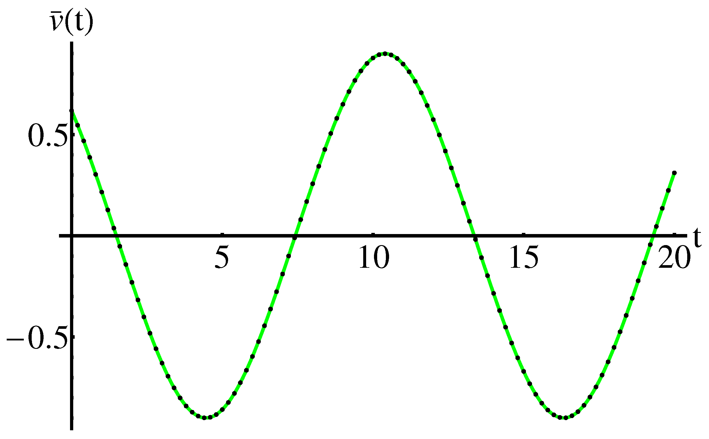
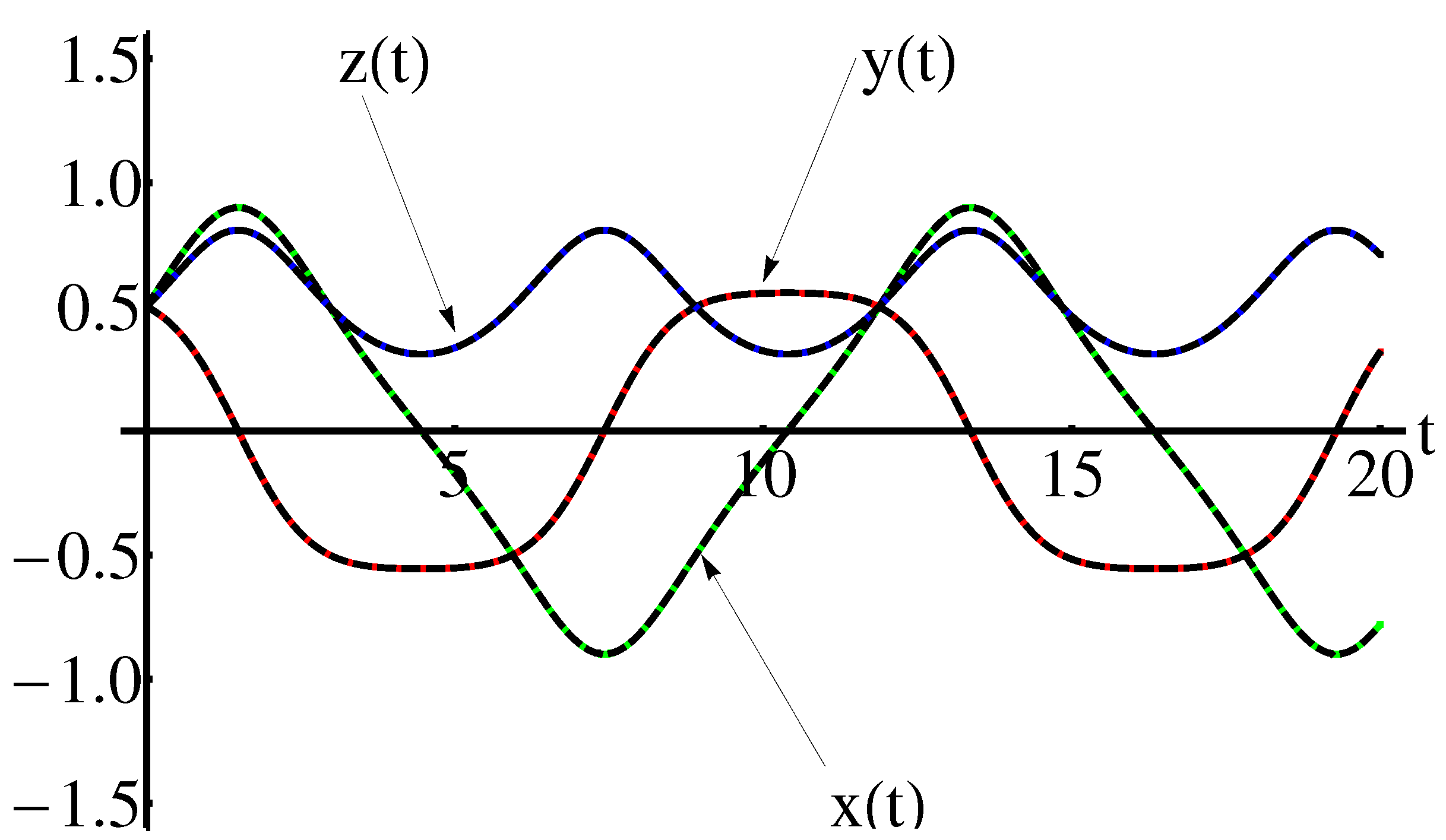
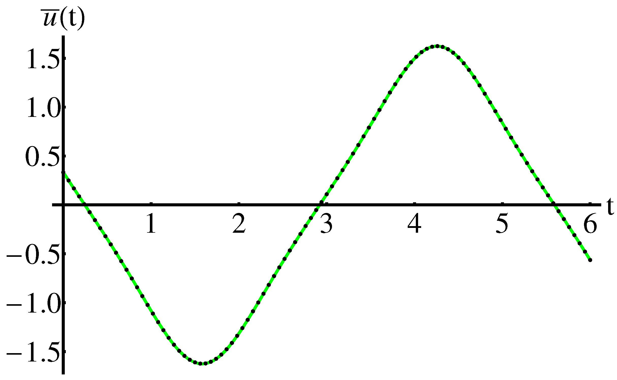
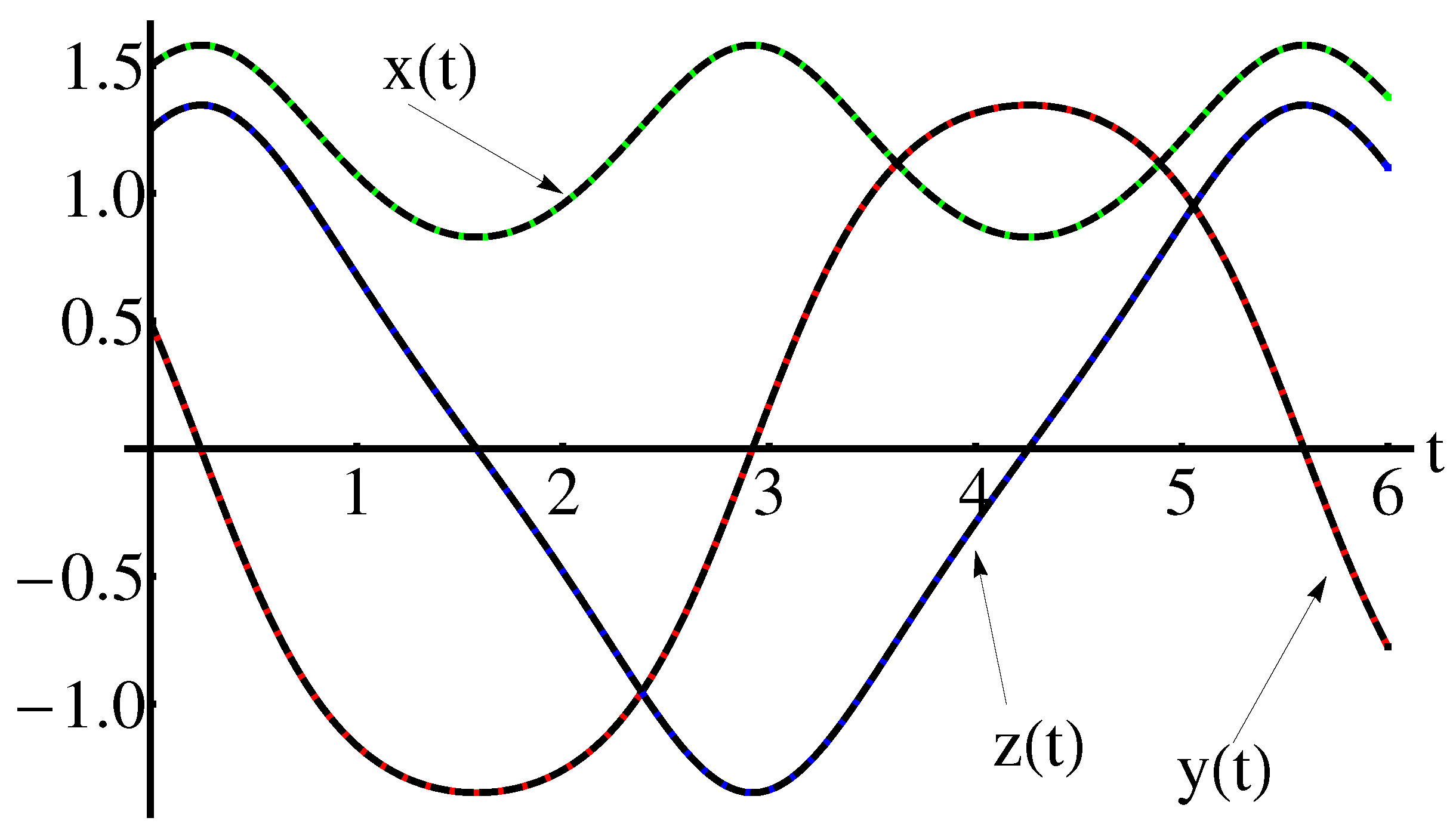
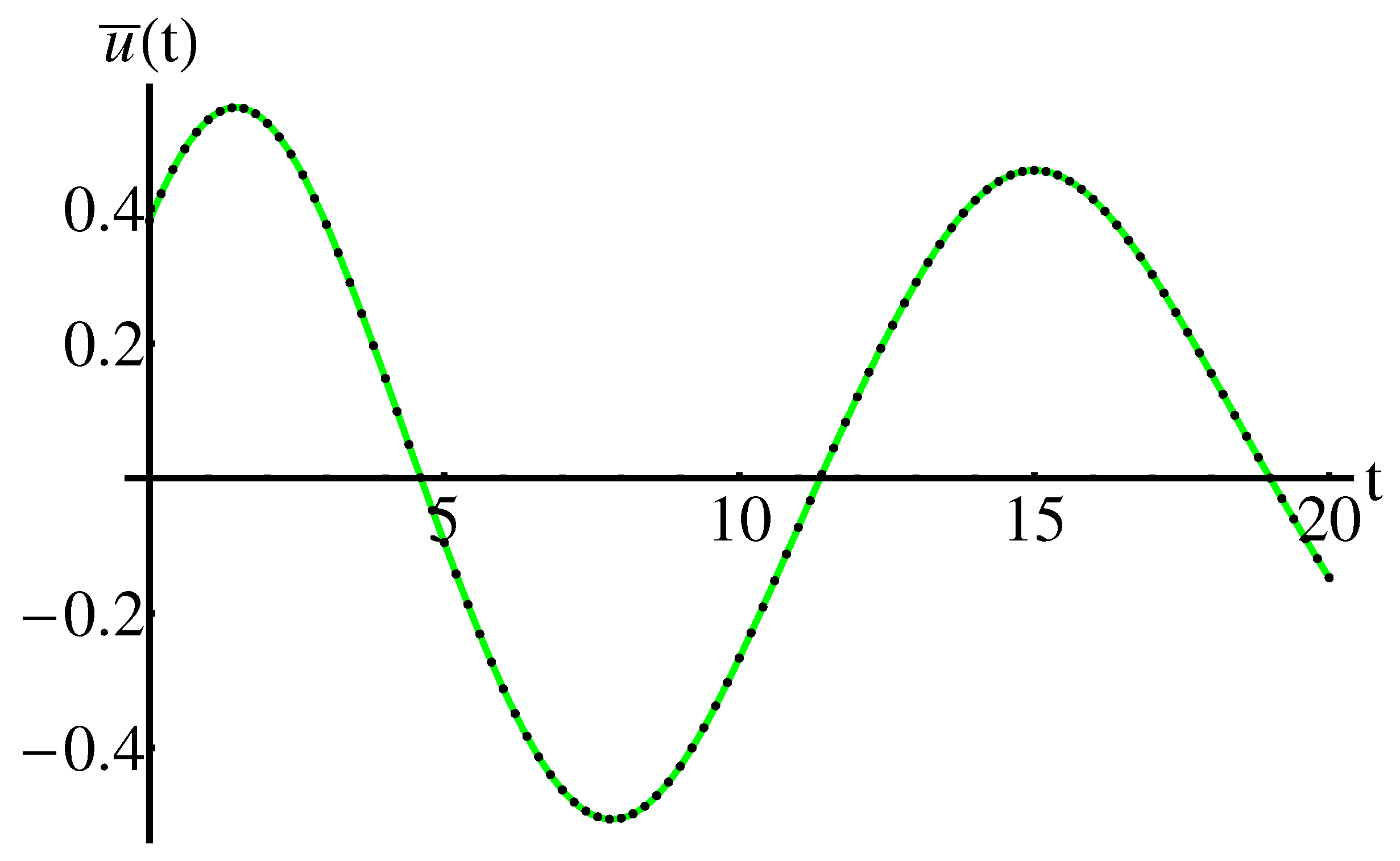
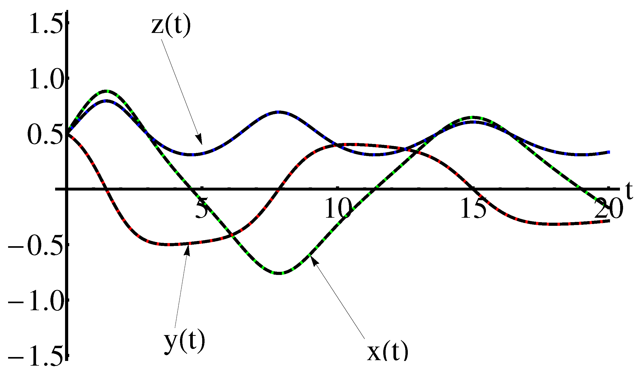
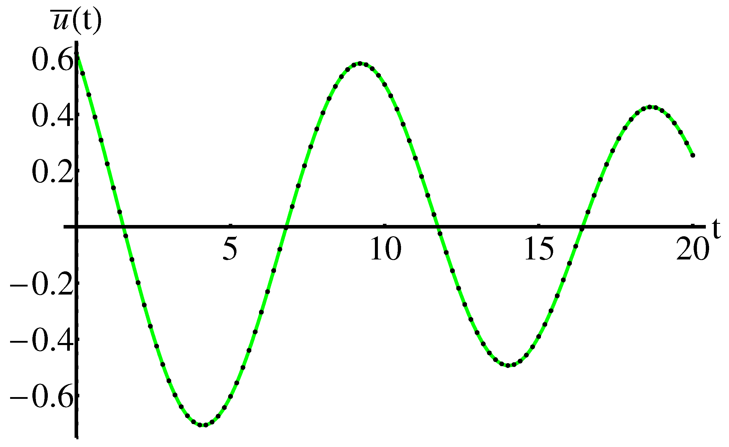
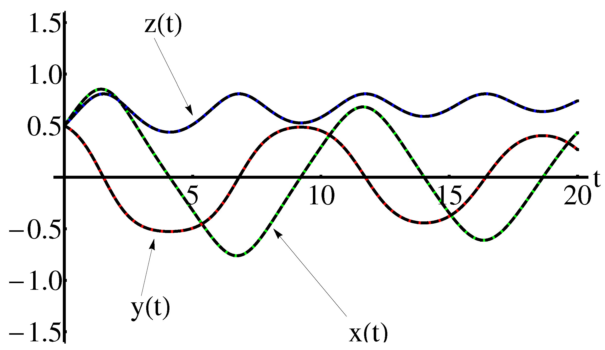
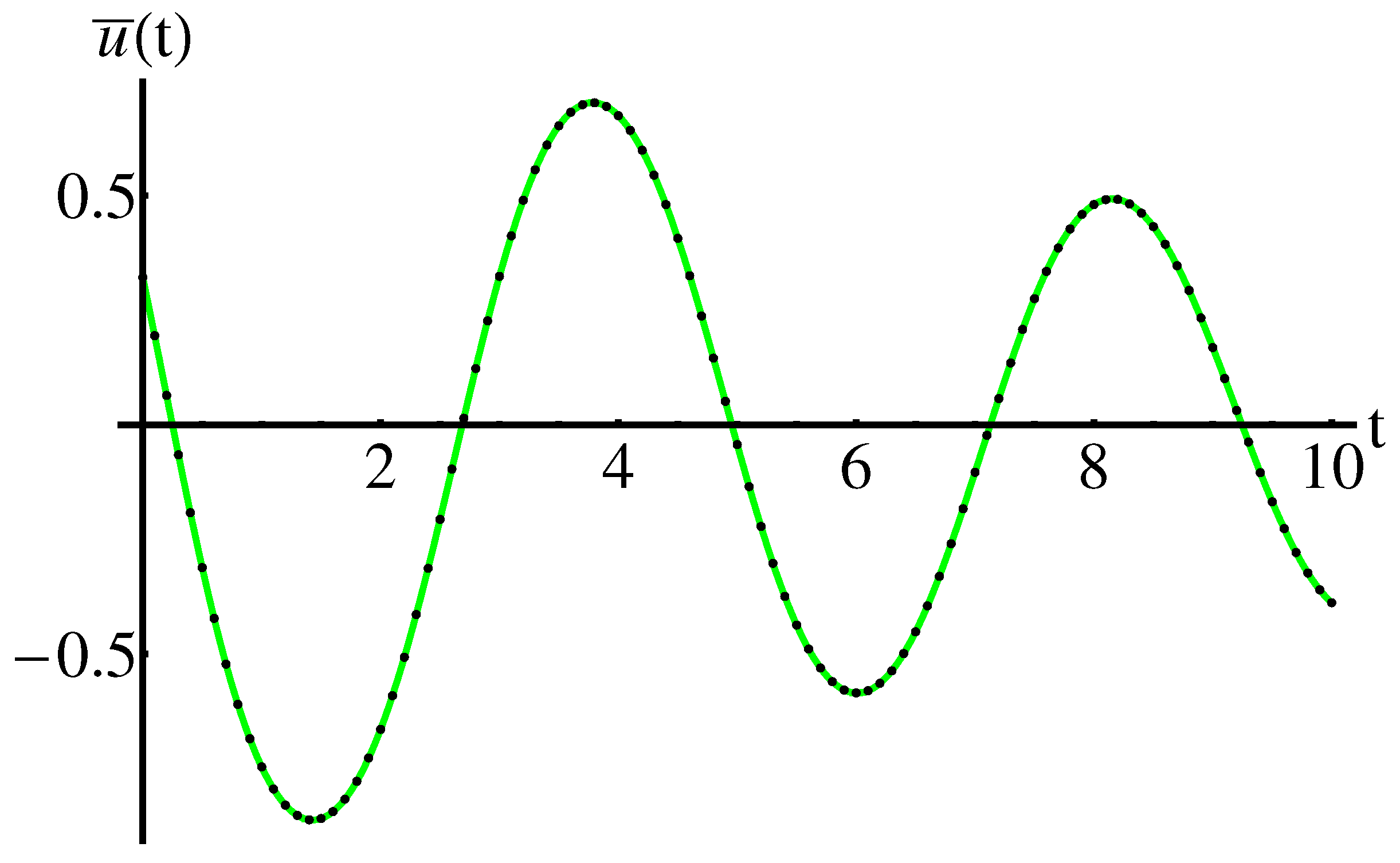
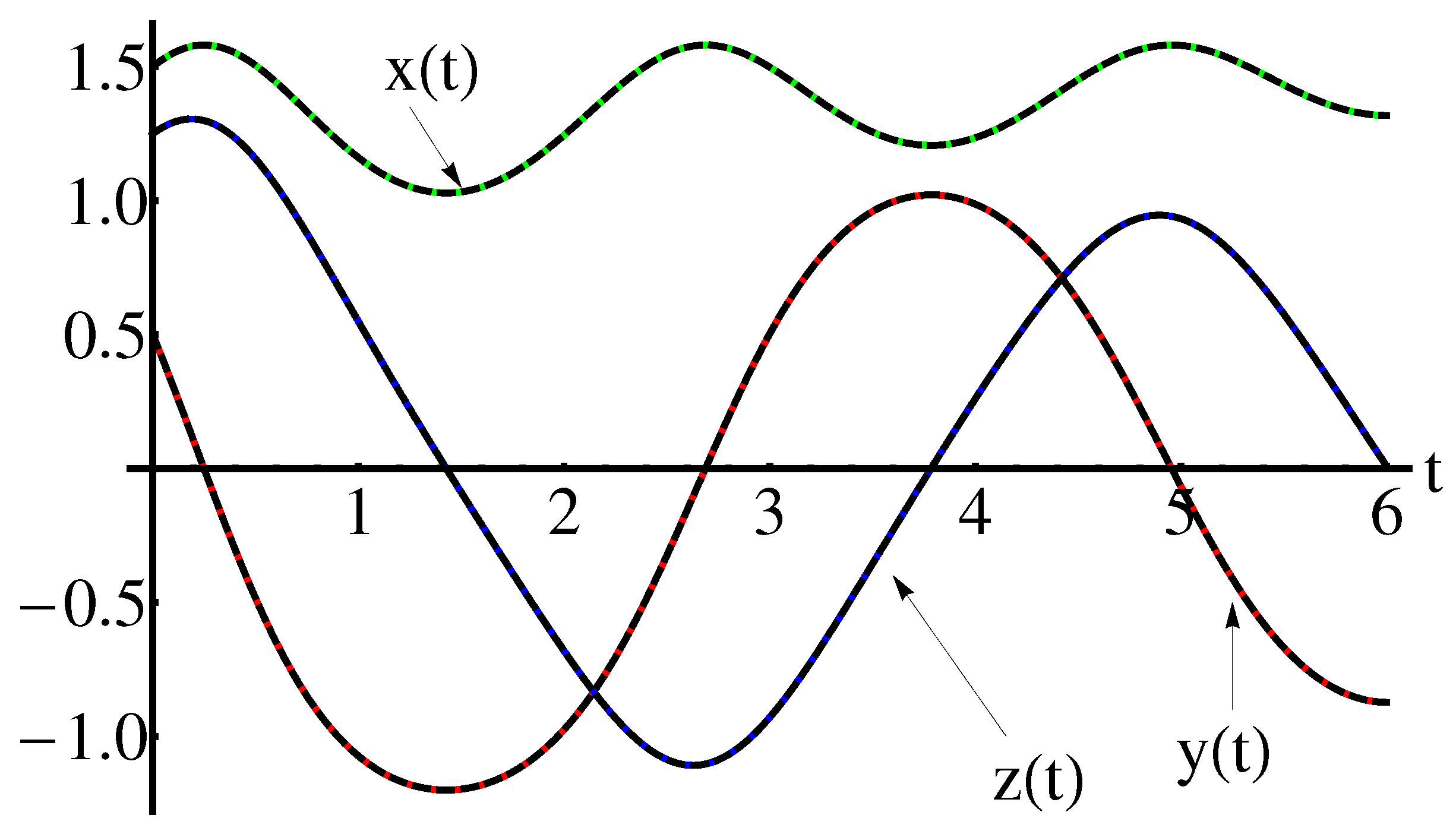
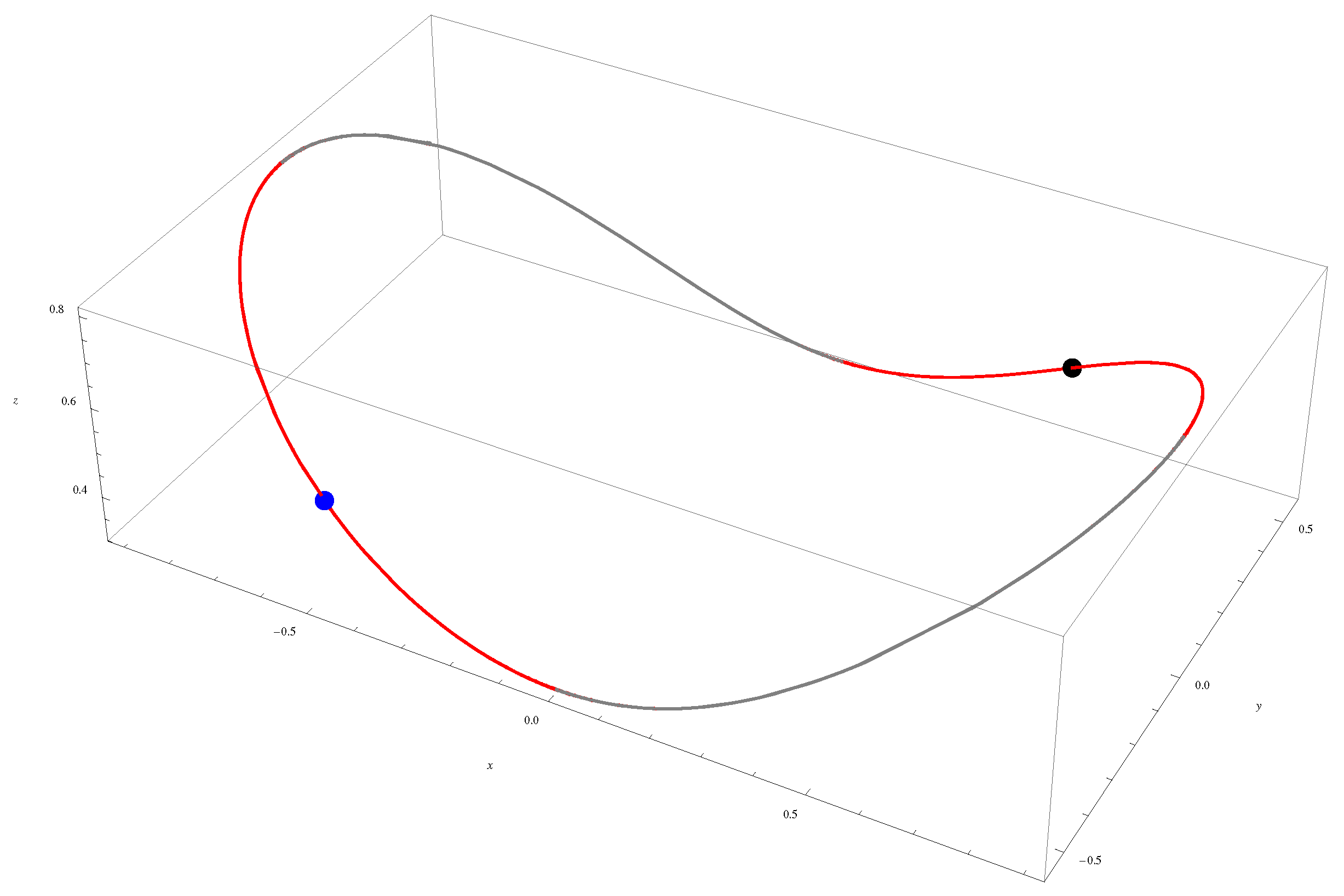
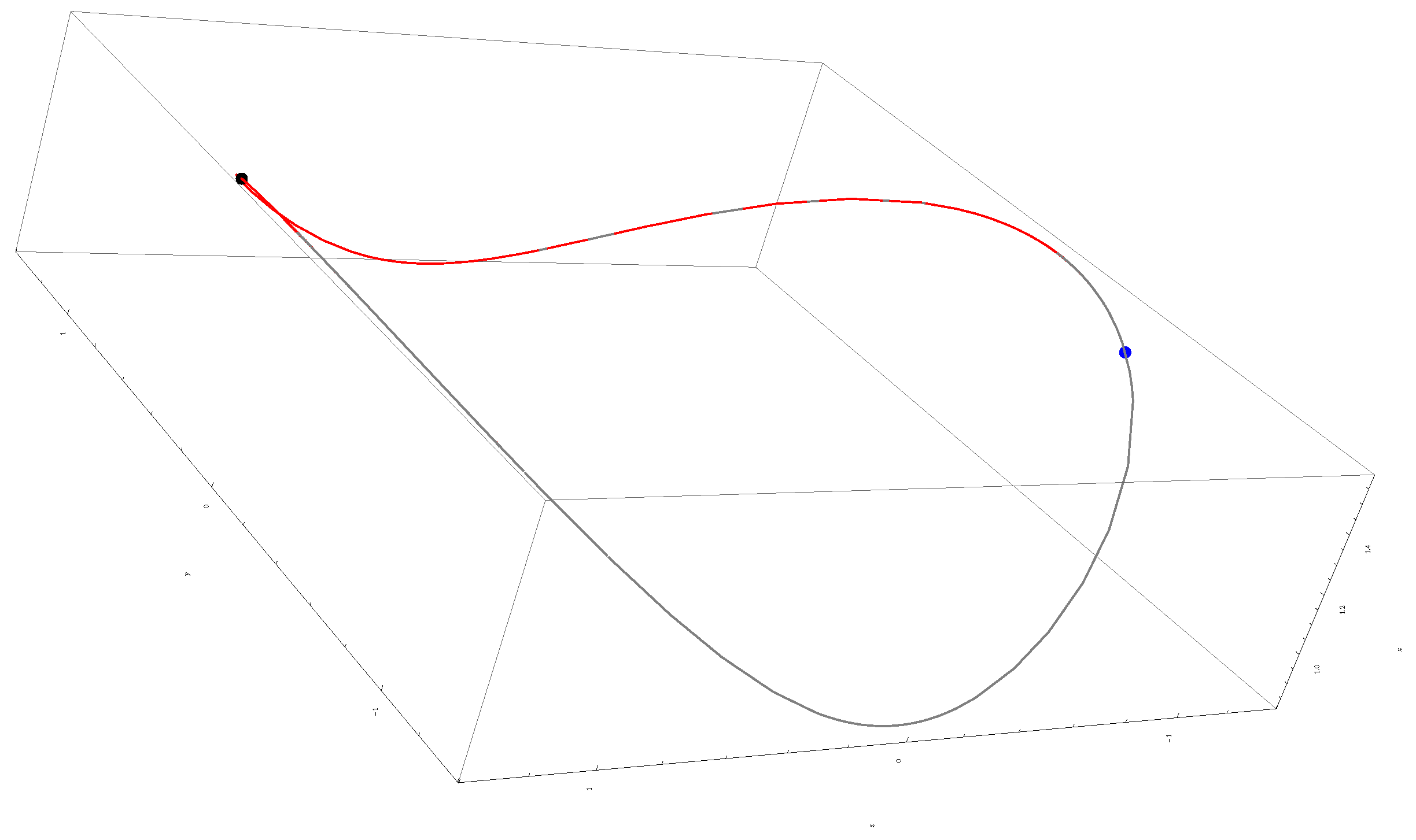
4. Numerical Results and Discussions

In this section, we discuss the accuracy of the OAFM method by taking into consideration the first order approximate solutions given by Equations (40) and (41), where the index N m a x { 10 , 15 , 25 , 35 } is an arbitrary fixed positive integer number.
By means of the Equations (3), (4), (40), for β 0 , α 1 = 0 , α 2 = 0 , α 3 = 0 , the Equations (8), (9), (41), for β = 0 , α 1 = 0 , α 2 = 0 , α 3 = 0 , the Equations (12), (14), (40), for α 1 = 0 , α 2 0 , α 3 = 0 , the Equations (16), (17), (40), for α 1 0 , α 2 = 0 , α 3 = 0 , and the Equations (19), (20), (42), for α 1 = 0 , β = 0 , α 2 = 0 , α 3 0 , respectively, the approximate closed-form solutions of the Rabinovich system are well-determined, via the OAFM technique.
The accuracy of the obtained results is shown in the Figure 1 and Figure 2 (for β = 0.25 0 , α 1 = 0 , α 2 = 0 , α 3 = 0 ), the Figure 3 and Figure 4 (for β = 0 , α 1 = 0 , α 2 = 0 , α 3 = 0 ) respectively, by comparison of the above obtained approximate solutions with the corresponding numerical integration results, computed by means of the fourth-order Runge-Kutta method using Wolfram Mathematica 9.0 software. On the other hand, the cases α 1 0 , α 2 0 , α 3 0 are depicted in Figure 5, Figure 6, Figure 7, Figure 8, Figure 9 and Figure 10. The convergence-control parameters C 1 = a 0 + v ( 0 ) , C i = a k 1 ( 4 ) , B 1 = b 0 + v ˙ ( 0 ) ω 0 , B i = b k 1 ( 4 ) , i = 2 , 3 , N m a x , which appear in Equations (40)–(42) are optimally identified by the least square method for different values of the known parameter N m a x . As could be observed in the figures there are the symmetry with respect to the O z - axis, for β 0 , α 1 = 0 , α 2 = 0 , α 3 = 0 and are the symmetry with respect to the all coordinate axes, for β = 0 , α 1 = 0 , α 2 = 0 , α 3 = 0 . The Figure 11 and Figure 12 highlight the symmetry of the 3D trajectory.
The convergence-control parameters are presented in the section Appendix A.
The influence of the index number N m a x on the values of the relative errors is examined in Table 1 and Table 2. The better approximate analytical solution corresponds to the value N m a x = 25 for β = 0.25 , α 1 = 0 , α 2 = 0 , α 3 = 0 , and N m a x = 35 for β = 0 , α 1 = 0 , α 2 = 0 , α 3 = 0 , respectively. These values were chosen for the efficiency of the solutions shown in Table 3, Table 4 and Table 5.

5. Conclusions

In the present paper, some geometrical properties of the Rabinovich system are emphasized and the approximate analytic solutions were established. These analytic solutions depend on some convergence-control parameters. A good agreement between the approximate analytic solutions (using OAFM) and corresponding numerical solutions (using the fourth-order Runge-Kutta method) was found for symmetric solutions with respect to the coordinate axes. The performance of the method is characterized by suitable values of the parameter N m a x as shown in the Tables and Figures. These obtained solutions can be used in many applications of technological interest. The advantage is to obtain accurate solutions for special cases, with just an analytic first integral known, but the unknown exact solution (as the intersection of the surfaces).

Author Contributions

Conceptualization, R.-D.E. and N.P.; methodology, N.P.; software, R.-D.E. and N.P.; validation, R.-D.E. and N.P.; formal analysis, R.-D.E., N.P. and M.L.; investigation, R.-D.E., N.P. and M.L.; writing—original draft preparation, R.-D.E., N.P. and M.L.; writing—review and editing, R.-D.E., N.P. and M.L.; visualization, R.-D.E., N.P. and M.L.; supervision, N.P. All authors have read and agreed to the published version of the manuscript.

Funding

This research received no external funding.

Conflicts of Interest

The authors declare no conflict of interest.

Appendix A

In the following we will present just the values of the convergence-control parameters that appear in Equations (40), (41) and (42), respectively.

Appendix A.1. The Case β ≠ 0, α1 = 0, α2 = 0, α3 = 0

Example A1.
The initial conditions are x 0 = 0.5 , y 0 = 0.5 , z 0 = 0.5 and β = 0.25 .
(a) for Equation (40) with N m a x = 10 :
ω 0 = 0.0842084063 , B 1 = 7.7850095373 , B 2 = 1.1935759266 , B 3 = 10.9766341996 , B 4 = 1.0576315879 , B 5 = 5.5540946245 , B 6 = 1.3916077665 , B 7 = 1.2287912091 , B 8 = 0.3774505937 , B 9 = 0.0856590499 , B 10 = 0.0177125387 , C 1 = 1.2647924166 , C 2 = 9.8753733548 , C 3 = 0.2632330456 , C 4 = 8.4861481647 , C 5 = 1.5913245793 , C 6 = 2.9461688979 , C 7 = 0.8568908158 , C 8 = 0.3803812033 , C 9 = 0.1212724374 , C 10 = 0.0080186284 ;
(b) for Equation (40) with N m a x = 15 :
ω 0 = 0.0842084063 , B 1 = 7.8470508367 , B 2 = 2.2499897809 , B 3 = 12.9280127794 , B 4 = 0.4712356520 , B 5 = 9.7259134278 , B 6 = 1.3690509281 , B 7 = 4.4434866499 , B 8 = 1.1492580188 , B 9 = 1.1762526193 , B 10 = 0.3861053828 , B 11 = 0.1603359895 , B 12 = 0.0563660451 , B 13 = 0.0090989642 , B 14 = 0.0027442264 , B 15 = 2.773923 · 10 6 , C 1 = 1.6353827930 , C 2 = 10.5668121613 , C 3 = 1.8492817431 , C 4 = 11.8272674286 , C 5 = 0.7138152947 , C 6 = 7.0224266784 , C 7 = 1.4476285900 , C 8 = 2.4512890639 , C 9 = 0.7451197226 , C 10 = 0.4745313849 , C 11 = 0.1651164438 , C 12 = 0.0436858802 , C 13 = 0.0147119639 , C 14 = 0.0012846915 , C 15 = 0.0004718731 ;
(c) for Equation (40) with N m a x = 25 :
ω 0 = 0.0842084063 , B 1 = 113.1906313266 , B 2 = 700.5143533516 , B 3 = 63.8042262780 , B 4 = 1726.7156941065 , B 5 = 727.2541799033 , B 6 = 1850.2472856376 , B 7 = 1458.7090868963 , B 8 = 1023.3252919624 , B 9 = 1371.45280473155 , B 10 = 192.8265190738 , B 11 = 763.9333733724 , B 12 = 118.7239396963 , B 13 = 261.2640026833 , B 14 = 98.9226990064 , B 15 = 51.1015243215 , B 16 = 33.0902447676 , B 17 = 3.9323646180 , B 18 = 5.8957249378 , B 19 = 0.3704710427 , B 20 = 0.5357572940 , B 21 = 0.0886533581 , B 22 = 0.0195324516 , B 23 = 0.0045186018 , B 24 = 0.0001056260 , B 25 = 0.0000356013 , C 1 = 237.0082862136 , C 2 = 181.1626337930 , C 3 = 1260.1800896233 , C 4 = 266.1579780903 , C 5 = 1943.0958639398 , C 6 = 1170.9065813163 , C 7 = 1501.3433857085 , C 8 = 1520.5635275053 , C 9 = 554.5650629146 , C 10 = 1087.6826289541 , C 11 = 26.0903663084 , C 12 = 475.6102111380 , C 13 = 128.1837256078 , C 14 = 125.1740070213 , C 15 = 62.1706696066 , C 16 = 16.9073998070 , C 17 = 15.0951778584 , C 18 = 0.2064815885 , C 19 = 1.9508776536 , C 20 = 0.2353541523 , C 21 = 0.1178869685 , C 22 = 0.0237146201 , C 23 = 0.0021457461 , C 24 = 0.0005641598 , C 25 = 3.317757 · 10 6 .
Now, for the initial conditions x 0 = 0.5 , y 0 = 0.5 , z 0 = 0.5 and N m a x = 25 , β = 0.25 the convergence-control parameters for the symmetric solution (with respect to the O z -axis) given by Equation (40) are given in Equation (A3).

Appendix A.2. The Remarkable Case β = 0, α1 = 0, α2 = 0, α3 = 0

Example A2.
The initial conditions are x 0 = 1.5 , y 0 = 0.5 , z 0 = 1.25 .
(a) for Equation (41) with N m a x = 15 :
ω 0 = 0.1869876739 , B 1 = 554.4037761129 , B 2 = 226.7457730999 , B 3 = 782.3721160745 , B 4 = 48.5974967462 , B 5 = 49.4030334587 , B 6 = 957.7117203144 , B 7 = 283.2006105162 , B 8 = 159.1917408848 , B 9 = 674.7077918425 , B 10 = 23.5125177445 , B 11 = 495.1189399730 , B 12 = 141.3482748307 , B 13 = 50.5506946689 , B 14 = 16.7536940267 , B 15 = 0.0634441781 , C 1 = 93.4671025566 , C 2 = 1047.0086776914 , C 3 = 495.9436000281 , C 4 = 133.5434805609 , C 5 = 746.4077270771 , C 6 = 236.7019711439 , C 7 = 421.4165739752 , C 8 = 177.1891806165 , C 9 = 254.4730564674 , C 10 = 758.0078082782 , C 11 = 147.8047599915 , C 12 = 204.0625242583 , C 13 = 66.0059654899 , C 14 = 6.0287025308 , C 15 = 1.8659955242 ;
(b) for Equation (41) with N m a x = 25 :
ω 0 = 0.1869876739 , B 1 = 516.1242386938 , B 2 = 370.2739755607 , B 3 = 438.3744282729 , B 4 = 232.6309328533 , B 5 = 282.3256743841 , B 6 = 387.5617017331 , B 7 = 47.8049293623 , B 8 = 162.7251241075 , B 9 = 117.3367937705 , B 10 = 59.7546990652 , B 11 = 111.8077188524 , B 12 = 71.8237012001 , B 13 = 149.4299059907 , B 14 = 60.2531991051 , B 15 = 76.3055734495 , B 16 = 113.6663413024 , B 17 = 16.3900394802 , B 18 = 108.9340003143 , B 19 = 91.5339247140 , B 20 = 72.0679666456 , B 21 = 67.2469830900 , B 22 = 0.6349607714 , B 23 = 7.3149658364 , B 24 = 0.8138266745 , B 25 = 0.0661089513 , C 1 = 54.6954626367 , C 2 = 889.6642684770 , C 3 = 678.0047311577 , C 4 = 235.8685894546 , C 5 = 401.5470307526 , C 6 = 43.0268550584 , C 7 = 40.6366633629 , C 8 = 169.6938622093 , C 9 = 23.4686692840 , C 10 = 115.4282122040 , C 11 = 73.1279637248 , C 12 = 92.7226387177 , C 13 = 55.3435319845 , C 14 = 12.4804646698 , C 15 = 67.0157693986 , C 16 = 29.4365871710 , C 17 = 9.0367780737 , C 18 = 25.8911752609 , C 19 = 126.8226917481 , C 20 = 103.3382634787 , C 21 = 20.0135321168 , C 22 = 27.9178547423 , C 23 = 2.5193238481 , C 24 = 1.0883135883 , C 25 = 0.0948041290 ;
(c) for Equation (41) with N m a x = 35 :
ω 0 = 0.1869876739 , B 1 = 27.1589347487 , B 2 = 12.0827987658 , B 3 = 31.2924026686 , B 4 = 6.2126489550 , B 5 = 8.4925801994 , B 6 = 13.9924569422 , B 7 = 6.0373789169 , B 8 = 19.7307983361 , B 9 = 1.4098763264 , B 10 = 23.1824059776 , B 11 = 19.5047102382 , B 12 = 18.0959242465 , B 13 = 20.3437872078 , B 14 = 2.3657500207 , B 15 = 8.0506645554 , B 16 = 2.1157429592 , B 17 = 8.2577036885 , B 18 = 24.5293827842 , B 19 = 9.7431739692 , B 20 = 13.3366939523 , B 21 = 21.0972405836 , B 22 = 1.3733966515 , B 23 = 10.4215638468 , B 24 = 0.6346613181 , B 25 = 3.7660664321 , B 26 = 6.3989961662 , B 27 = 14.1834202800 , B 28 = 8.4270149394 , B 29 = 5.0794721575 , B 30 = 6.5727871915 , B 31 = 1.2212175488 , B 32 = 0.6570547398 , B 33 = 0.2354677108 , B 34 = 0.0056214482 , B 35 = 0.0026220746 , C 1 = 19.7054442097 , C 2 = 54.4346582382 , C 3 = 0.8103617202 , C 4 = 1.8697297809 , C 5 = 5.5410468189 , C 6 = 4.1456744599 , C 7 = 25.1576973040 , C 8 = 4.3010254027 , C 9 = 18.3207242611 , C 10 = 9.5312211886 , C 11 = 21.8263082280 , C 12 = 20.0001654379 , C 13 = 14.6586935042 , C 14 = 21.2392716691 , C 15 = 9.2030700586 , C 16 = 10.5290971616 , C 17 = 24.7946288753 , C 18 = 8.9376532008 , C 19 = 1.1913707498 , C 20 = 8.9900769507 , C 21 = 8.2043548306 , C 22 = 16.8096509190 , C 23 = 1.8558514640 , C 24 = 8.7834639788 , C 25 = 5.1597513330 , C 26 = 6.9589549263 , C 27 = 0.6370483091 , C 28 = 12.0432828958 , C 29 = 10.0288355195 , C 30 = 0.0799417017 , C 31 = 2.6893238533 , C 32 = 0.7569825071 , C 33 = 0.0695529173 , C 34 = 0.0388832605 , C 35 = 0.0017247410 .
Now, for the initial conditions: x 0 = 1.5 , y 0 = 0.5 , z 0 = 1.25 (symmetry with respect to the O z -axis) and N m a x = 35 , β = 0 , x 0 = 1.5 , y 0 = 0.5 , z 0 = 1.25 (symmetry with respect to the O x -axis) and N m a x = 35 , β = 0 , x 0 = 1.5 , y 0 = 0.5 , z 0 = 1.25 (symmetry with respect to the O y -axis) and N m a x = 35 , β = 0 , the convergence-control parameters for the symmetric solution (with respect to the O z -axis) given by Equation (41) are given in Equation (A6).

Appendix A.3. The Case β = 0.25, α1 = 0, α2 = 0.05, α3 = 0

Example A3.
The initial conditions are x 0 = 0.5 , y 0 = 0.5 , z 0 = 0.5 and N m a x = 25 .
The convergence-control parameters for the approximate analytic solution u ¯ ( t ) given by Equation (40) are:
ω 0 = 0.0694543429 , B 1 = 69.5705751030 , B 2 = 120.8993887304 , B 3 = 134.8567394227 , B 4 = 80.2715486367 , B 5 = 133.5091139810 , B 6 = 1.6079535511 , B 7 = 107.8296608169 , B 8 = 89.0630671934 , B 9 = 153.5628496068 , B 10 = 103.8865887516 , B 11 = 81.7020914138 , B 12 = 124.0154016728 , B 13 = 71.0190829276 , B 14 = 279.0140436547 , B 15 = 47.4832381804 , B 16 = 186.4926850959 , B 17 = 1.6034548489 , B 18 = 58.0109625378 , B 19 = 5.9577818217 , B 20 = 8.6271212497 , B 21 = 1.2371738255 , B 22 = 0.5383432616 , B 23 = 0.0738473761 , B 24 = 0.0093636835 , B 25 = 0.0006547226 , C 1 = 65.0212060551 , C 2 = 146.9430296120 , C 3 = 122.0164695356 , C 4 = 12.7416766751 , C 5 = 35.4755424788 , C 6 = 188.0064243933 , C 7 = 37.3549977788 , C 8 = 42.6527153638 , C 9 = 125.7222674988 , C 10 = 160.3454312782 , C 11 = 9.0512355641 , C 12 = 14.4067469635 , C 13 = 234.7064480557 , C 14 = 74.8990251987 , C 15 = 253.4010415854 , C 16 = 16.8710869660 , C 17 = 113.8065189746 , C 18 = 7.2254321395 , C 19 = 24.6401183173 , C 20 = 3.1759631665 , C 21 = 2.4394846206 , C 22 = 0.3573106958 , C 23 = 0.0874588482 , C 24 = 0.0098968427 , C 25 = 0.0005010425 .

Appendix A.4. The Case β = 0.25, α1 = 0.05, α2 = 0, α3 = 0

Example A4.
The initial conditions are x 0 = 0.5 , y 0 = 0.5 , z 0 = 0.5 and N m a x = 25 .
The convergence-control parameters for the approximate analytic solution u ¯ ( t ) given by Equation (40) are:
ω 0 = 0.0979970641 , B 1 = 7.86946701639623 , B 2 = 6.4646829651 , B 3 = 8.7356943964 , B 4 = 16.3328135131 , B 5 = 5.1958788407 , B 6 = 10.8702566280 , B 7 = 12.6215405753 , B 8 = 1.5426658313 , B 9 = 6.8534549134 , B 10 = 5.3338415271 , B 11 = 0.1190016122 , B 12 = 2.4166370753 , B 13 = 1.2668179431 , B 14 = 0.1849844809 , B 15 = 0.4668487148 , B 16 = 0.1558661112 , B 17 = 0.0410984637 , B 18 = 0.0439753213 , B 19 = 0.0079302657 , B 20 = 0.0031640290 , B 21 = 0.0015152397 , B 22 = 0.0000782713 , B 23 = 0.0000586884 , B 24 = 7.908883 · 10 6 , B 25 = 2.571457 · 10 7 , C 1 = 1.7097438990 , C 2 = 10.0351472420 , C 3 = 12.4760001691 , C 4 = 2.2874375788 , C 5 = 15.6734001521 , C 6 = 10.8070637066 , C 7 = 4.2334673452 , C 8 = 10.7552729215 , C 9 = 4.7764382238 , C 10 = 2.8811116370 , C 11 = 4.1426512477 , C 12 = 1.1302932517 , C 13 = 0.9994302741 , C 14 = 0.8951531888 , C 15 = 0.1235578694 , C 16 = 0.1781342705 , C 17 = 0.0986544376 , C 18 = 0.0025652300 , C 19 = 0.0143255850 , C 20 = 0.0043772770 , C 21 = 0.0003038516 , C 22 = 0.0003624506 , C 23 = 0.0000398691 , C 24 = 5.795421 · 10 6 , C 25 = 7.292742 · 10 7 .

Appendix A.5. The Case β = 0, α1 = 0, α2 = 0, α3 = 0.15

Example A5.
The initial conditions are x 0 = 1.5 , y 0 = 0.5 , z 0 = 1.25 and N m a x = 35 .
The convergence-control parameters for the approximate analytic solution u ¯ ( t ) given by Equation (42) are:
ω 0 = 0.2172006104 , B 1 = 7.3251070555 , B 2 = 0.1087849966 , B 3 = 4.1113264263 , B 4 = 4.21373739429 , B 5 = 1.0687156558 , B 6 = 1.5599721276 , B 7 = 1.43202796290 , B 8 = 0.7373618607 , B 9 = 2.3909438155 , B 10 = 1.77937304336 , B 11 = 0.5409997087 , B 12 = 2.5317090264 , B 13 = 2.67997580834 , B 14 = 1.1492629171 , B 15 = 0.6922268586 , B 16 = 1.59791789658 , B 17 = 1.3153031289 , B 18 = 0.4470104143 , B 19 = 0.2651316628 , B 20 = 0.4881158033 , B 21 = 0.3386938091 , B 22 = 0.0985227111 , B 23 = 0.0470955155 , B 24 = 0.0741216873 , B 25 = 0.0431448916 , B 26 = 0.0106926238 , B 27 = 0.0035675339 , B 28 = 0.0047137818 , B 29 = 0.0021456860 , B 30 = 0.0004138394 , B 31 = 0.0000775657 , B 32 = 0.0000738535 , B 33 = 0.0000199500 , B 34 = 1.929570 · 10 8 , B 35 = 8.095036 · 10 8 , C 1 = 4.8320147836 , C 2 = 6.1545928815 , C 3 = 2.7172376117 , C 4 = 0.9374420135 , C 5 = 2.9359918166 , C 6 = 1.5185091234 , C 7 = 0.9997803324 , C 8 = 1.8049281860 , C 9 = 0.1894325635 , C 10 = 2.1155718115 , C 11 = 2.9032537901 , C 12 = 1.5215478343 , C 13 = 0.7804328110 , C 14 = 2.2301227152 , C 15 = 2.0399788427 , C 16 = 0.7655400005 , C 17 = 0.4739199152 , C 18 = 0.9603870342 , C 19 = 0.7236971824 , C 20 = 0.2267309158 , C 21 = 0.1229722256 , C 22 = 0.2088434889 , C 23 = 0.1332553039 , C 24 = 0.0359490437 , C 25 = 0.0146330134 , C 26 = 0.0212551967 , C 27 = 0.0111045215 , C 28 = 0.0024764806 , C 29 = 0.0006442642 , C 30 = 0.0007496569 , C 31 = 0.0002808121 , C 32 = 0.0000431036 , C 33 = 4.960082 · 10 6 , C 34 = 3.110982 · 10 6 , C 35 = 3.647933 · 10 7 .

References

  1. Pikovskii, A.S.; Rabinovich, M.I. Stochastic behavior of dissipative systems. Soc. Sci. Rev. C Math. Phys. Rev. 1981, 2, 165–208. [Google Scholar]
  2. Pikovskii, A.S.; Rabinovich, M.I.; Trakhtengerts, V.Y. Onset of stochasticity in decay confinement of parametric instability. Soc. Phys. JETP 1978, 47, 715–719. [Google Scholar]
  3. Kuznetsov, N.V.; Leonov, G.A.; Mokaev, T.N.; Seledzhi, S.M. Hidden attractor in the Rabinovich system, Chua circuits and PLL. AIP Conf. Proc. 2016, 1738, 210008. [Google Scholar] [CrossRef]
  4. Xiang, Z. Integrals of motion of the Rabinovich system. J. Phys. A Math. Gen. 2000, 33, 5137. [Google Scholar] [CrossRef]
  5. Tudoran, R.M.; Girban, A. On the Hamiltonian dynamics and geometry of the Rabinovich system. Discrete Cont. Dyn.-B 2011, 15, 789–823. [Google Scholar] [CrossRef]
  6. Xie, F.; Zhang, X. Invariant algebraic surfaces of the Rabinovich system. J. Phys. A Math. Gen. 2003, 36, 499. [Google Scholar] [CrossRef]
  7. Kocamaz, U.E.; Uyaroglu, Y.; Kizmaz, H. Control of Rabinovich chaotic system using sliding mode control. Int. J. Adapt. Control 2013, 28, 1413–1421. [Google Scholar] [CrossRef]
  8. Lazureanu, C.; Caplescu, C. Stabilization of the T system by an integrable deformation. In Proceedings of the International Conference on Applied Mathematics and Numerical Methods Third Edition, Craiova, Romania, 29–31 October 2020. [Google Scholar] [CrossRef]
  9. Braga, D.C.; Scalco, D.F.; Mello, L.F. On the stability of the equilibria of the Rikitake system. Phys. Lett. A 2010, 374, 4316–4320. [Google Scholar] [CrossRef]
  10. Rikitake, T. Oscillations of a system of disk dynamos. Proc. Camb. Philos. Soc. 1958, 54, 89–105. [Google Scholar] [CrossRef]
  11. Steeb, W.H. Continuous symmetries of the Lorenz model and the Rikitake two-disc dynamo system. J. Phys. A Math. Gen. 1982, 15, 389–390. [Google Scholar] [CrossRef]
  12. Binzar, T.; Lazureanu, C. On the symmetries of a Rabinovich type system. Sci. Bull. Math.-Phys. 2012, 57, 29–36. [Google Scholar]
  13. Lazureanu, C.; Binzar, T. Symmetries of some classes of dynamical systems. J. Nonlinear Math. Phys. 2015, 22, 265–274. [Google Scholar] [CrossRef]
  14. Lazureanu, C.; Petrisor, C.; Hedrea, C. On a deformed version of the two-disk dynamo system. Appl. Math. 2021, 66, 345–372. [Google Scholar] [CrossRef]
  15. Lazureanu, C.; Petrisor, C. Stability and energy-Casimir Mapping for integrable deformations of the Kermack-McKendrick system. Adv. Math. Phys. 2018, 2018, 5398768. [Google Scholar] [CrossRef]
  16. Lazureanu, C. Integrable deformations of three-dimensional chaotic systems. Int. J. Bifurcat. Chaos 2018, 28, 71850066. [Google Scholar] [CrossRef]
  17. Lazureanu, C. Hamilton-Poisson realizations of the integrable deformations of the Rikitake system. Adv. Math. Phys. 2017, 2017, 4596951. [Google Scholar] [CrossRef] [Green Version]
  18. Lazureanu, C. The real-valued Maxwell-Bloch equations with controls: From a Hamilton-Poisson system to a chaotic one. Int. J. Bifurcat. Chaos 2017, 27, 1750143. [Google Scholar] [CrossRef]
  19. Lazureanu, C. On a Hamilton-Poisson approach of the Maxwell-Bloch equations with a control. Math. Phys. Anal. Geom. 2017, 3, 20. [Google Scholar] [CrossRef]
  20. Lazureanu, C.; Binzar, T. Symmetries and properties of the energy-Casimir mapping in the ball-plate problem. Adv. Math. Phys. 2017, 2017, 5164602. [Google Scholar] [CrossRef] [Green Version]
  21. Lazureanu, C.; Binzar, T. On some properties and symmetries of the 5-dimensional Lorenz system. Math. Probl. Eng. 2015, 2015, 438694. [Google Scholar] [CrossRef]
  22. Lazureanu, C.; Binzar, T. Some symmetries of a Rossler type system. Sci. Bull. Math.-Phys. 2013, 58, 1–6. [Google Scholar]
  23. Binzar, T.; Lazureanu, C. A Rikitake type system with one control. Discrete Contin. Dyn. Syst.-B 2013, 18, 1755–1776. [Google Scholar] [CrossRef]
  24. Lazureanu, C.; Binzar, T. Symplectic realizations and symmetries of a Lotka-Volterra type system. Regul. Chaotic Dyn. 2013, 18, 203–213. [Google Scholar] [CrossRef]
  25. Lazureanu, C.; Binzar, T. A Rikitake type system with quadratic control. Int. J. Bifurcat. Chaos 2012, 22, 1250274. [Google Scholar] [CrossRef]
  26. Lazureanu, C.; Binzar, T. On the symmetries of a Rikitake type system. C. R. Math. Acad. Sci. Paris 2012, 350, 529–533. [Google Scholar] [CrossRef] [Green Version]
  27. Lazureanu, C. On the Hamilton-Poisson realizations of the integrable deformations of the Maxwell-Bloch equations. C. R. Math. Acad. Sci. Paris 2017, 355, 596–600. [Google Scholar] [CrossRef]
  28. Candido Murilo, R.; Llibre, J.; Valls, C. New symmetric periodic solutions for the Maxwell-Bloch differential system. Math. Phys. Anal. Geom. 2019, 22, 16. [Google Scholar] [CrossRef]
  29. Liu, Y.; Yang, Q.; Pang, G. A hyperchaotic system from the Rabinovich system. J. Comput. Appl. Math. 2010, 234, 101–113. [Google Scholar] [CrossRef] [Green Version]
  30. David, D.; Holm, D. Multiple Lie–Poisson structures, reduction and geometric phases for the Maxwell–Bloch traveling wave equations. J. Nonlinear Sci. 1992, 2, 241–262. [Google Scholar] [CrossRef]
  31. Puta, M. On the Maxwell–Bloch equations with one control. C. R. Math. Acad. Sci. Paris 1994, 318, 679–683. [Google Scholar]
  32. Puta, M. Three dimensional real valued Maxwell–Bloch equations with controls. Rep. Math. Phys. 1996, 37, 337–348. [Google Scholar] [CrossRef]
  33. Arecchi, F.T. Chaos and generalized multistability in quantum optics. Phys. Scr. 1985, 9, 85–92. [Google Scholar] [CrossRef]
  34. Casu, I.; Lazureanu, C. Stability and integrability aspects for the Maxwell-Bloch equations with the rotating wave approximation. Regul. Chaotic Dyn. 2017, 22, 109–121. [Google Scholar] [CrossRef]
  35. Zuo, D.W. Modulation instability and breathers synchronization of the nonlinear Schrodinger Maxwell–Bloch equation. Appl. Math. Lett. 2018, 79, 182–186. [Google Scholar] [CrossRef]
  36. Wang, L.; Wang, Z.Q.; Sun, W.R.; Shi, Y.Y.; Li, M.; Xu, M. Dynamics of Peregrine combs and Peregrine walls in an inhomogeneous Hirota and Maxwell–Bloch system. Commun. Nonlinear Sci. 2017, 47, 190–199. [Google Scholar] [CrossRef]
  37. Wei, J.; Wang, X.; Geng, X. Periodic and rational solutions of the reduced Maxwell–Bloch equations. Commun. Nonlinear Sci. 2018, 59, 1–14. [Google Scholar] [CrossRef] [Green Version]
  38. Binzar, T.; Lazureanu, C. On some dynamical and geometrical properties of the Maxwell–Bloch equations with a quadratic control. J. Geom. Phys. 2013, 70, 1–8. [Google Scholar] [CrossRef]
  39. Puta, M. Integrability and geometric prequantization of the Maxwell-Bloch equations. Bull. Sci. Math. 1998, 122, 243–250. [Google Scholar] [CrossRef] [Green Version]
  40. Llibre, J.; Valls, C. Global analytic integrability of the Rabinovich system. J. Geom. Phys. 2008, 58, 1762–1771. [Google Scholar] [CrossRef]
  41. Herisanu, N.; Marinca, V. Accurate analytical solutions to oscillators with discontinuities and fractional-power restoring force by means of the optimal homotopy asymptotic method. Comput. Math. Appl. 2010, 60, 1607–1615. [Google Scholar] [CrossRef] [Green Version]
  42. Marinca, V.; Herisanu, N. The Optimal Homotopy Asymptotic Method—Engineering Applications; Springer: Heidelberg, Germany, 2015. [Google Scholar]
  43. Marinca, V.; Herisanu, N. An application of the optimal homotopy asymptotic method to Blasius problem. Rom. J. Tech. Sci. Appl. Mech. 2015, 60, 206–215. [Google Scholar]
  44. Marinca, V.; Herisanu, N. Nonlinear dynamic analysis of an electrical machine rotor-bearing system by the optimal homotopy perturbation method. Comp. Math. Appl. 2011, 61, 2019–2024. [Google Scholar] [CrossRef] [Green Version]
  45. Marinca, V.; Ene, R.D.; Marinca, B. Optimal Homotopy Perturbation Method for nonlinear problems with applications. Appl. Comp. Math. 2022, 21, 123–136. [Google Scholar]
  46. Turkyilmazoglu, M. An optimal variational iteration method. Appl. Math. Lett. 2011, 24, 762–765. [Google Scholar] [CrossRef] [Green Version]
  47. Marinca, V.; Draganescu, G.E. Construction of approximate periodic solutions to a modified van der Pol oscillator. Nonlinear Anal. Real World Appl. 2010, 11, 4355–4362. [Google Scholar] [CrossRef]
  48. Caruntu, B.; Bota, C.; Lapadat, M.; Pasca, M.S. Polynomial Least Squares Method for Fractional Lane-Emden Equations. Symmetry 2019, 11, 479. [Google Scholar] [CrossRef]
  49. Bota, C.; Caruntu, B.; Tucu, D.; Lapadat, M.; Pasca, M.S. A Least Squares Differential Quadrature Method for a Class of Nonlinear Partial Differential Equations of Fractional Order. Mathematics 2020, 8, 1336. [Google Scholar] [CrossRef]
  50. Amer, T.S.; Bek, M.A.; Hassan, S.S.; Elbendary, S. The stability analysis for the motion of a nonlinear damped vibrating dynamical system with three-degrees-of-freedom. Results Phys. 2021, 28, 104561. [Google Scholar] [CrossRef]
  51. El-Rashidy, K.; Seadawy Aly, R.; Saad, A.; Makhlou, M.M. Multiwave, Kinky breathers and multi-peak soliton solutions for the nonlinear Hirota dynamical system. Results Phys. 2020, 19, 103678. [Google Scholar] [CrossRef]
  52. Hussain, S.; Shah, A.; Ayub, S.; Ullah, A. An approximate analytical solution of the Allen-Cahn equation using homotopy perturbation method and homotopy analysis method. Heliyon 2019, 5, e03060. [Google Scholar] [CrossRef] [Green Version]
  53. Wang, X.; Xu, Q.; Atluri, S.N. Combination of the variational iteration method and numerical algorithms for nonlinear problems. Appl. Math. Model. 2020, 79, 243–259. [Google Scholar] [CrossRef]
  54. Marinca, V.; Herisanu, N. Approximate analytical solutions to Jerk equation. In Springer Proceedings in Mathematics & Statistics: Proceedings of the Dynamical Systems: Theoretical and Experimental Analysis, Lodz, Poland, 7–10 December 2015; Springer: Cham, Switzerland, 10 December 2016; Volume 182, pp. 169–176. [Google Scholar]
Figure 1. The auxiliary function v ¯ ( t ) given by Equations (40) and (A3) using the initial conditions x 0 = 0.5 , y 0 = 0.5 , z 0 = 0.5 and β = 0.25 , α 1 = 0 , α 2 = 0 , α 3 = 0 for N m a x = 25 : OAFM solution (with lines) and numerical solution (dashing lines), respectively.
Symmetry 14 02185 g001
Figure 2. The set of solutions x ( t ) , y ( t ) , z ( t ) given by Equations (3) and (4) using Equations (40) and (A3) with the initial conditions x 0 = 0.5 , y 0 = 0.5 , z 0 = 0.5 and β = 0.25 , α 1 = 0 , α 2 = 0 , α 3 = 0 for N m a x = 25 : OAFM solution (with lines) and numerical solution (dashing lines), respectively.
Symmetry 14 02185 g002
Figure 3. The auxiliary function u ¯ ( t ) given by Equations (41) and (A6) using the initial conditions x 0 = 1.5 , y 0 = 0.5 , z 0 = 1.25 and β = 0 , α 1 = 0 , α 2 = 0 , α 3 = 0 for N m a x = 35 : OAFM solution (with lines) and numerical solution (dashing lines), respectively.
Symmetry 14 02185 g003
Figure 4. The set of solutions x ( t ) , y ( t ) , z ( t ) given by Equations (8) and (9) using Equations (41) and (A6) with the initial conditions x 0 = 1.5 , y 0 = 0.5 , z 0 = 1.25 and β = 0 , α 1 = 0 , α 2 = 0 , α 3 = 0 for N m a x = 35 : OAFM solution (with lines) and numerical solution (dashing lines), respectively.
Symmetry 14 02185 g004
Figure 5. The auxiliary function u ¯ ( t ) given by Equations (40) and (A7) using the initial conditions x 0 = 0.5 , y 0 = 0.5 , z 0 = 0.5 and β = 0.25 , α 1 = 0 , α 2 = 0.05 , α 3 = 0 for N m a x = 25 : OAFM solution (with lines) and numerical solution (dashing lines), respectively.
Symmetry 14 02185 g005
Figure 6. The set of solutions x ( t ) , y ( t ) , z ( t ) given by Equations (12) and (14) using Equations (40) and (A7) with the initial conditions x 0 = 0.5 , y 0 = 0.5 , z 0 = 0.5 and β = 0.25 , α 1 = 0 , α 2 = 0.05 , α 3 = 0 for N m a x = 25 : OAFM solution (with lines) and numerical solution (dashing lines), respectively.
Symmetry 14 02185 g006
Figure 7. The auxiliary function u ¯ ( t ) given by Equations (40) and (A8) using the initial conditions x 0 = 0.5 , y 0 = 0.5 , z 0 = 0.5 and β = 0.25 , α 1 = 0.05 , α 2 = 0 , α 3 = 0 for N m a x = 25 : OAFM solution (with lines) and numerical solution (dashing lines), respectively.
Symmetry 14 02185 g007
Figure 8. The set of solutions x ( t ) , y ( t ) , z ( t ) given by Equations (16) and (17) using Equations (40) and (A8) with the initial conditions x 0 = 0.5 , y 0 = 0.5 , z 0 = 0.5 and β = 0.25 , α 1 = 0.05 , α 2 = 0 , α 3 = 0 for N m a x = 25 : OAFM solution (with lines) and numerical solution (dashing lines), respectively.
Symmetry 14 02185 g008
Figure 9. The auxiliary function u ¯ ( t ) given by Equations (42) and (A9) using the initial conditions x 0 = 1.5 , y 0 = 0.5 , z 0 = 1.25 and β = 0 , α 1 = 0 , α 2 = 0 , α 3 = 0.15 for N m a x = 35 : OAFM solution (with lines) and numerical solution (dashing lines), respectively.
Symmetry 14 02185 g009
Figure 10. The set of solutions x ( t ) , y ( t ) , z ( t ) given by Equations (19) and (20) using Equations (42) and (A9) with the initial conditions x 0 = 1.5 , y 0 = 0.5 , z 0 = 1.25 and β = 0 , α 1 = 0 , α 2 = 0 , α 3 = 0.15 for N m a x = 35 : OAFM solution (with lines) and numerical solution (dashing lines), respectively.
Symmetry 14 02185 g010
Figure 11. The points ( 0.5 , 0.5 , 0.5 ) (black), ( 0.5 , 0.5 , 0.5 ) (blue) and the parametric 3D curve x = x ( t ) , y = y ( t ) , z = z ( t ) given by Equations (3) and (4) using Equations (40), (A3) with the initial conditions x 0 = 0.5 , y 0 = 0.5 , z 0 = 0.5 and β = 0.25 , α 1 = 0 , α 2 = 0 , α 3 = 0 for N m a x = 25 : OAFM solution (with gray line) and numerical solution (dashing red line), respectively.
Symmetry 14 02185 g011
Figure 12. The points ( 1.5 , 0.5 , 1.25 ) (black), ( 1.5 , 0.5 , 1.25 ) (blue) and the parametric 3D curve x = x ( t ) , y = y ( t ) , z = z ( t ) given by Equations (8) and (9) using Equations (41) and (A6) with the initial conditions x 0 = 1.5 , y 0 = 0.5 , z 0 = 1.25 and β = 0 , α 1 = 0 , α 2 = 0 , α 3 = 0 for N m a x = 35 : OAFM solution (with gray line) and numerical solution (dashing red line), respectively.
Symmetry 14 02185 g012
Table 1. Comparison between the relative errors: ϵ v = | v n u m e r i c a l v ¯ O A F M | for β = 0.25 , α 1 = 0 , α 2 = 0 , α 3 = 0 , x 0 = 0.5 , y 0 = 0.5 , z 0 = 0.5 and different values of the index N m a x ; v ¯ O A F M obtained from Equations (40) and (A1)–(A3).
t N max = 10 N max = 15 N max = 25
01.332267 × 10 15 4.440892 × 10 16 2.646771 × 10 13
7/50.00023117019.690649 × 10 7 5.424820 × 10 10
14/50.00014947439.806902 × 10 7 3.389437 × 10 10
21/50.00019871021.243573 × 10 6 1.842952 × 10 10
28/50.00009616995.341956 × 10 8 6.126734 × 10 10
70.00012104842.545193 × 10 6 4.273881 × 10 10
42/50.00006616531.815027 × 10 6 2.335903 × 10 10
49/59.306109 × 10 6 2.151637 × 10 6 5.521745 × 10 10
56/50.00002117902.055369 × 10 6 4.816658 × 10 10
63/50.00015109442.318730 × 10 7 7.166223 × 10 11
140.00019196231.595892 × 10 6 1.900378 × 10 10
Table 2. Comparison between the relative errors: ϵ u = | u n u m e r i c a l u ¯ O A F M | for β = 0 , α 1 = 0 , α 2 = 0 , α 3 = 0 , x 0 = 1.5 , y 0 = 0.5 , z 0 = 1.25 and different values of the index N m a x ; u ¯ O A F M obtained from Equations (41) and (A4)–(A6).
t N max = 15 N max = 25 N max = 35
09.475753 × 10 14 1.587063 × 10 13 7.716050 × 10 15
3/53.504900 × 10 4 3.316779 × 10 5 8.194535 × 10 8
6/52.914220 × 10 4 2.904368 × 10 5 7.775160 × 10 8
9/54.067788 × 10 4 3.306752 × 10 5 1.002242 × 10 7
12/55.020959 × 10 4 3.350227 × 10 5 1.013316 × 10 7
32.399299 × 10 4 3.095774 × 10 5 6.350594 × 10 8
18/57.499806 × 10 5 3.033164 × 10 5 9.363366 × 10 8
21/52.634217 × 10 4 3.698857 × 10 5 7.855941 × 10 8
24/51.023441 × 10 4 3.459891 × 10 5 2.951037 × 10 8
27/51.061241 × 10 4 3.200782 × 10 5 4.558553 × 10 8
61.528191 × 10 4 3.492756 × 10 5 5.671638 × 10 8
Table 3. Comparison between the approximate analytic solutions u ¯ O A F M given by Equation (40) and corresponding numerical solution for β = 0.25 , α 1 = 0 , α 2 = 0.05 , α 3 = 0 , x 0 = 0.5 , y 0 = 0.5 , z 0 = 0.5 and the index N m a x = 25 ; (relative errors: ϵ u = | u n u m e r i c a l u ¯ O A F M | ).
t u numerical u ¯ OAFM ϵ u
00.38196601120.38196601126.566969 × 10 14
8/50.54871988760.54871988714.569626 × 10 10
16/50.33475666200.33475666244.373337 × 10 10
24/5−0.0474300084−0.04743000749.474402 × 10 10
32/5−0.3828045448−0.38280454502.316530 × 10 10
8−0.5042437854−0.50424378381.624801 × 10 9
48/5−0.3375790298−0.33757902998.105455 × 10 11
56/5−0.0332606638−0.03326066468.140353 × 10 10
64/50.25997407180.25997407223.694533 × 10 10
72/50.44073837940.44073837984.701539 × 10 10
160.41402156150.41402156105.571915 × 10 10
Table 4. Comparison between the approximate analytic solutions u ¯ O A F M given by Equation (40) and corresponding numerical solution for β = 0.25 , α 1 = 0.05 , α 2 = 0 , α 3 = 0 , x 0 = 0.5 , y 0 = 0.5 , z 0 = 0.5 and the index N m a x = 25 ; (relative errors: ϵ u = | u n u m e r i c a l u ¯ O A F M | ).
t u numerical u ¯ OAFM ϵ u
00.61803398870.61803398878.881784 × 10 16
8/5−0.0321978118−0.03219781107.381383 × 10 10
16/5−0.5983010647−0.59830106452.040423 × 10 10
24/5−0.6430063264−0.64300632651.829493 × 10 10
32/5−0.1556677170−0.15566771663.093710 × 10 10
80.40570188410.40570188329.304779 × 10 10
48/50.56266799380.56266799413.481130 × 10 10
56/50.17918653000.17918652946.380252 × 10 10
64/5−0.3292856584−0.32928565776.622721 × 10 10
72/5−0.4774573136−0.47745731351.349091 × 10 10
16−0.1296948250−0.12969482518.001704 × 10 11
Table 5. Comparison between the approximate analytic solutions u ¯ O A F M given by Equation (42) and corresponding numerical solution for β = 0 , α 1 = 0 , α 2 = 0 , α 3 = 0.15 , x 0 = 1.5 , y 0 = 0.5 , z 0 = 1.25 and the index N m a x = 35 ; (relative errors: ϵ u = | u n u m e r i c a l u ¯ O A F M | ).
t u numerical = 15 u ¯ OAFM ϵ u
00.32175055430.32175055431.665334 × 10 16
3/5−0.4222547682−0.42225614021.371977 × 10 6
6/5−0.8296437373−0.82964511621.378897 × 10 6
9/5−0.7776543854−0.77765576731.381888 × 10 6
12/5−0.3129872607−0.31298864231.381552 × 10 6
30.32390448220.32390310311.379085 × 10 6
18/50.68159035930.68158897521.384109 × 10 6
21/50.59893872850.59893734731.381160 × 10 6
24/50.14533666720.14533528551.381609 × 10 6
27/5−0.3742949616−0.37429633981.378268 × 10 6
6−0.5850269138−0.58502828511.371267 × 10 6
Publisher’s Note: MDPI stays neutral with regard to jurisdictional claims in published maps and institutional affiliations.

