The Reliability of Stored Water behind Dams Using the Multi-Component Stress-Strength System

Abstract

Dams are essential infrastructure for managing water resources and providing entry to clean water for human needs. However, the construction and maintenance of dams require careful consideration of their reliability and safety, specifically in the event of extreme weather conditions such as heavy rainfall or flooding. In this study, the stress-strength model provides a useful framework for evaluating the reliability of dams and their ability to cope with external stresses such as water pressure, earthquake activity, and erosion. The Shasta reservoir in the United States is a prime example of a dam that requires regular assessment of its reliability to guarantee the safety of communities and infrastructure. The Gumbel Type II distribution has been suggested as a suitable model for fitting the collected data on the stress and strength of the reservoir behind the Shasta dam. Both classical and Bayesian approaches have been used to estimate the reliability function under the multi-component stress-strength model, and Monte Carlo simulation has been employed for parameter estimation. In addition, some measures of goodness-of-fit are employed to examine the suitability of the suggested model.

1. Introduction

In reliability analysis, the study of the failure time of a component or a system is of great concern. Decision-makers in industry or governments encourage continuity in the enhancement of systems reliability since it measures the functioning of systems and predicts their outcomes in a better way. One of the main problems is estimating the parameters of the stress-strength function $R=P(Y<X)$, where Y is the stress and X is the strength, and both are considered random variables. Components or systems are subject to failure if their strength is less than the stress applied to them at any time.

Statistical inference of the stress-strength function has been studied by many authors. Several lifetime distributions were considered to fit the model under consideration, such as Birnbaum [1], Hanagal [2], Kotz et al. [3], Raqab et al. [4], Kundu and Raqab [5], Lio and Tsai [6], Nadar et al. [7], Rao and Kantam [8], Rao [9], Rao [10], Rao et al. [11], Kizilaslan and Nadar [12], Nadar and Kizilaslan [13], Dey et al. [14], and Wu [15]. For more recent works one may refer to [16,17,18,19,20,21].

A multi-component system, with k-independent and identically distributed (iid) strength components and one common stress, is in a functional state if at least s components are surviving at the same time, where $1\le s\le k$, and this is known as an s-out-of-k: G system. Two examples of multi-component systems are: first, the suspension bridge is suspended by a k-vertical cable pair, this bridge will survive if at least s-vertical cable pairs are functioning, i.e., not damaged. Second, the engine with six cylinders will work properly if at least four out of six cylinders are functioning.

Estimating the reliability of a system with the multi-component stress-strength model is of great importance and has many applications, see for example Ahmad et al. [22], who used the Power Lomax distribution under a progressive censoring scheme. Johari et al. [23] studied the reliability analysis of ground soil layers using the cross-correlation method. More reliability inference studies are presented in [24,25].

In this work, we consider the stress-strength model applied to reservoirs or artificial lakes behind dams. Dams are very important for providing water for different purposes during droughts such as drinking, cooking, washing, and irrigation, as well as producing hydroelectric power. They help in storing water in reservoirs during excess water flow and release it during times of low flow. Besides irrigation and other consumption purposes, water stored in these reservoirs is subject to other loss factors such as evaporation. We consider a model that is related to excessive drought times, and it is also claimed that in a specific region, if the stored water in a reservoir in August of the previous year is less than the water amount in the reservoir for at least two of the next four years, then no excessive drought will occur. In this model, X represents the strength and Y represents the stress.

In this study, we aim to estimate the stress-strength function’s parameters $R_{s,k}$ which follow the Gumbel Type II model. This model was invented in 1958 by the German mathematician Emil Gumbel (1891–1911) and was useful for predicting the likelihood of climatic events such as annual flood flows (which is the case of this study), earthquakes, and other natural disasters. According to Abbas et al. [26], it has also been demonstrated to be sufficient for describing the component’s life expectancy. In their book, Kotz and Nadarajah [27] investigated the Gumbel distribution with the aim of applying it to the analysis of datasets ranging from wind speed to flood data.

Several authors focused on the Gumbel Type II distribution in their research for its wide range of applications. For example, Nadarajah and Kotz [28] studied the Gumbel distribution’s main properties. Feroze and Muhammad [29] performed Bayesian inference for the Gumbel Type II distribution under twice censored samples with different loss functions. Mansour and Aboshady [30] discussed different estimation methods using the Gumbel Type II distribution under the hybrid Type II censored scheme, they applied this model to study the performance of the insulating fluids for the breakdown voltages.

One of the basic motivations for using the Gumbel Type II distribution for modelling real data is its ability to keep the properties of a wide range of distributions, including the Weibull, Fréchet, and Gumbel distributions. This makes the Gumbel Type II distribution a flexible alternative for modelling data that are not compatible with some distributional forms. Another motivation for using the Gumbel Type II distribution is its ability to model both heavy-tailed and light-tailed distributions, as well as distributions that obtain positive or negative skewness. Moreover, the Gumbel Type II distribution is often used to model extreme events such as floods, hurricanes, and earthquakes, where accurate modelling of the distribution is essential for risk assessment and management. The Gumbel Type II distribution has been found to support a good fit for many extreme events, making it a preferable choice for modelling such events.

Even though several types of research have been performed on the statistical inference of the Gumbel Type II distribution, there is still a persistent need for more work in the field of multi-component stress-strength systems with Gumbel Type II distribution. In this study, we work on two goals: first, to find classical and Bayesian estimators of multi-component stress-strength functions and assess the estimators by providing a simulation study and applying suitable numerical techniques. Second, apply the new model to fit real data collected from reservoirs behind the Shasta dam.

The procedure for organizing the process of this work is schematically shown in the flowchart in Figure 1.

2. Reliability Function

In this section, a closed form is obtained for the reliability function for a stress-strength model. Assuming the probability density function (PDF) and the CDF for the Gumbel Type II distribution, with a random variable X defined as,

$$f\left(x\right)=\alpha \beta x^{-(\alpha +1)}{e}^{-\beta x^{-\alpha }},x>0,\alpha ,\beta >0.$$

(1)

and

$$F\left(x\right)=e^{-\beta x^{-\alpha }},x>0,\alpha ,\beta >0,$$

(2)

and given the reliability function for a stress-strength model, that was defined by Bhattacharyya and Johnson [31], as

$$R_{s,k}=P\left[\mathrm{at}\mathrm{least}s\mathrm{of}\right(X_1,X_2,\cdots ,X_k\left)\mathrm{exceed}Y\right]=\sum _{i=s}^k\left(\genfrac{}{}{0pt}{}{k}{i}\right){\int }_{-\infty }^{\infty }{[1-F\left(X\right)]}^i{\left[F\left(X\right)\right]}^{k-i}dG\left(Y\right),$$

(3)

where $X_1,X_2,\cdots ,X_k$ are iid random variables that follow the Gumbel Type II distribution with parameters ${\alpha }_1$ and ${\beta }_1$ with cumulative distribution function (CDF) $F\left(X\right)$, and are affected by random stresses Y that follow the Gumbel Type II distribution with parameters ${\alpha }_2$ and ${\beta }_2$ having CDF $G\left(Y\right)$. Substituting by the CDF in Equation (2) into $R_{s,k}$ defined in Equation (3), we obtain

$$R_{s,k}={\alpha }_2{\beta }_2\sum _{i=s}^k\left(\genfrac{}{}{0pt}{}{k}{i}\right){\int }_0^{\infty }{[1-e^{-{\beta }_1{x}^{-{\alpha }_1}}]}^i{\left[e^{-{\beta }_1{x}^{-{\alpha }_1}}\right]}^{k-i}{x}^{-({\alpha }_2+1)}{e}^{-{\beta }_2{x}^{-{\alpha }_2}}dx.$$

(4)

Let $u=x^{-{\alpha }_2}$ and substitute it into Equation (4) to obtain Equation (5)

$$R_{s,k}={\beta }_2\sum _{i=s}^k\left(\genfrac{}{}{0pt}{}{k}{i}\right){\int }_0^{\infty }{[1-e^{-{\beta }_1{u}^{\frac{{\alpha }_1}{{\alpha }_2}}}]}^i{\left[e^{-{\beta }_1{u}^{\frac{{\alpha }_1}{{\alpha }_2}}}\right]}^{k-i}{e}^{-{\beta }_{2}u}du.$$

(5)

By using the binomial expansion for $[1-e^{-{\beta }_1{u}^{\frac{{\alpha }_1}{{\alpha }_2}}}]$, we obtain

$$R_{s,k}={\beta }_2\sum _{i=s}^k\sum _{l=0}^i\left(\genfrac{}{}{0pt}{}{k}{i}\right)\left(\genfrac{}{}{0pt}{}{i}{l}\right){(-1)}^l{\int }_0^{\infty }{\left[e^{-{\beta }_1{u}^{\frac{{\alpha }_1}{{\alpha }_2}}}\right]}^{k-l}{e}^{-{\beta }_{2}u}du.$$

(6)

Since the Maclaurin expansion for ${\left[e^{-{\beta }_1{u}^{\frac{{\alpha }_1}{{\alpha }_2}}}\right]}^{k-l}={\sum }_{r=0}^{\infty }\frac{{(l-k)}^r{\beta }_1^r{u}^{\frac{r{\alpha }_1}{{\alpha }_2}}}{r!}$, then Equation (6) is rewritten as

$$R_{s,k}={\beta }_2\sum _{i=s}^k\sum _{l=0}^i\sum _{r=0}^{\infty }\left(\genfrac{}{}{0pt}{}{k}{i}\right)\left(\genfrac{}{}{0pt}{}{i}{l}\right){(-1)}^l\frac{{(l-k)}^r{\beta }_1^r}{r!}{\int }_0^{\infty }{u}^{\frac{r{\alpha }_1}{{\alpha }_2}}{e}^{-{\beta }_{2}u}du.$$

(7)

Assuming $z={\beta }_{2}u$, Equation (7) is reduced to

$$R_{s,k}=\sum _{i=s}^k\sum _{l=0}^i\sum _{r=0}^{\infty }\left(\genfrac{}{}{0pt}{}{k}{i}\right)\left(\genfrac{}{}{0pt}{}{i}{l}\right){(-1)}^l\frac{{(l-k)}^r{\beta }_1^r}{r!}{\beta }_2^{-\frac{r{\alpha }_1}{{\alpha }_2}}\Gamma \left(\frac{r{\alpha }_1}{{\alpha }_2}+1\right).$$

(8)

3. Maximum-Likelihood Estimation

This section is devoted to deriving the maximum likelihood estimators (MLEs) for the reliability function’s $R_{s,k}$ parameters. The basis for finding the estimators of the parameters is the log-likelihood functions, given the data. The MLEs have been used by many authors to derive the estimators of the parameters due to several advantages such as simplicity, unbiased for larger samples, and acquiring smaller variance. Furthermore, it can be developed for a large variety of other estimation methods. For more information on the likelihood theory, see Azzalini [32].

To find the MLEs of $R_{s,k}$, we start by obtaining the MLEs for the parameters ${\alpha }_1,{\alpha }_2,{\beta }_1$ and ${\beta }_2$. In this model, samples can be constructed as

     $\left(\begin{array}{cccc}{X}_{11}& X_{12}& \cdots & X_{1k}\\ X_{21}& X_{22}& \cdots & X_{2k}\\ ⋮& ⋮& \ddots & ⋮\\ X_{n1}& X_{n2}& \cdots & X_{nk}\end{array}\right)$    and    $\left(\begin{array}{c}{Y}_1\\ Y_2\\ ⋮\\ Y_n\end{array}\right)$

     Observed strength variables      Observed stress variables

Hence, the likelihood function for the observations can be written as

$$L({\alpha }_1,{\alpha }_2,{\beta }_1,{\beta }_2)=\prod _{i=1}^n\left[\prod _{j=1}^{k}f\left(x_{i,j}\right)\right]g\left(y_i\right),$$

(9)

where

$$\begin{array}{c}\hfill f\left(x_{ij}\right)={\alpha }_1{\beta }_1{x}_{ij}^{-({\alpha }_1+1)}{e}^{-{\beta }_1{x}_{ij}^{-{\alpha }_1}},\\ \hfill g\left(y_i\right)={\alpha }_2{\beta }_2{y}_i^{-({\alpha }_2+1)}{e}^{-{\beta }_2{y}_i^{-{\alpha }_2}}.\end{array}$$

Equation (9) can then be written as

$$L({\alpha }_1,{\alpha }_2,{\beta }_1,{\beta }_2)={\alpha }_1^{nk}{\alpha }_2^n{\beta }_1^{nk}{\beta }_2^n\left[\prod _{i=1}^n\prod _{j=1}^k{x}_{i,j}^{-{\alpha }_1-1}\right]\left[\prod _{i=1}^n{y}_i^{-{\alpha }_2-1}\right]\left[e^{-{\beta }_1{\sum }_{i=1}^n{\sum }_{j=1}^k{x}_{i,j}^{-{\alpha }_1}}\right]\left[e^{-{\beta }_2{\sum }_{i=1}^n{y}_i^{-{\alpha }_2}}\right].$$

(10)

From Equation (10), the log-likelihood function can be derived as follows

$$\begin{array}{ccc}\hfill \ell ({\alpha }_1,{\alpha }_2,{\beta }_1,{\beta }_2)& =& nk[log\left({\alpha }_1\right)+log\left({\beta }_1\right)]+n[log\left({\alpha }_2\right)+log\left({\beta }_2\right)]-({\alpha }_1+1)\left[\sum _{i=1}^n\sum _{j=1}^{k}log\left(x_{i,j}\right)\right]\hfill \\ \hfill & & \times ({\alpha }_2+1)\left[\sum _{i=1}^{n}log\left(y_i\right)\right]-{\beta }_1\left[\sum _{i=1}^n\sum _{j=1}^k{x}_{i,j}^{-{\alpha }_1}\right]-{\beta }_2\left[\sum _{i=1}^n{y}_i^{-{\alpha }_2}\right].\hfill \end{array}$$

(11)

Computing the first partial derivatives for ℓ with respect to ${\alpha }_1$, ${\alpha }_2$, ${\beta }_1$ and ${\beta }_2$ and equating with zero will give the four equations below

$$\frac{nk}{{\alpha }_1}-\left[\sum _{i=1}^n\sum _{j=1}^{k}log\left(x_{i,j}\right)\right]+{\beta }_1\left[\sum _{i=1}^n\sum _{j=1}^k{x}_{i,j}^{-{\alpha }_1}log\left(x_{i,j}\right)\right]=0,$$

(12)

$$\frac{n}{{\alpha }_2}-\left[\sum _{i=1}^{n}log\left(y_i\right)\right]+{\beta }_2\left[\sum _{i=1}^n{y}_i^{-{\alpha }_2}log\left(y_i\right)\right]=0,$$

(13)

$$\frac{nk}{{\beta }_1}-\left[\sum _{i=1}^n\sum _{j=1}^k{x}_{i,j}^{-{\alpha }_1}\right]=0,$$

(14)

$$\frac{n}{{\beta }_2}-\left[\sum _{i=1}^n{y}_i^{-{\alpha }_2}\right]=0,$$

(15)

Straightforward from Equations (14) and (15), the estimators for ${\beta }_1$ and ${\beta }_2$ can be given as

$${\widehat{\beta }}_1=\frac{nk}{{\sum }_{i=1}^n{\sum }_{j=1}^k{x}_{i,j}^{-{\widehat{\alpha }}_1}}\mathrm{and}{\widehat{\beta }}_2=\frac{n}{{\sum }_{i=1}^n{y}_i^{-{\widehat{\alpha }}_2}}$$

(16)

Dragging the two estimates in Equation (16) into Equations (12) and (13), respectively, and solving will give estimates for ${\alpha }_1$ and ${\alpha }_2$, ${\widehat{\alpha }}_1$ and ${\widehat{\alpha }}_2$, respectively, and substituting by ${\widehat{\alpha }}_1,{\widehat{\alpha }}_2,{\widehat{\beta }}_1$ and ${\widehat{\beta }}_2$ in Equation (8), we obtain the MLE ${\widehat{R}}_{s,k}$ as follows

$${\widehat{R}}_{s,k}=\sum _{i=s}^k\sum _{l=0}^i\sum _{r=0}^{\infty }\left(\genfrac{}{}{0pt}{}{k}{i}\right)\left(\genfrac{}{}{0pt}{}{i}{l}\right){(-1)}^l\frac{{(l-k)}^r{\widehat{\beta }}_1^r}{r!}{\widehat{\beta }}_2^{-\frac{r{\widehat{\alpha }}_1}{{\widehat{\alpha }}_2}}\Gamma \left(\frac{r{\widehat{\alpha }}_1}{{\widehat{\alpha }}_2}+1\right).$$

(17)

Fisher Information Matrix

In this sub-section, the asymptotic confidence interval (ACI) for the reliability function will be derived using the Fisher information (FI) matrix. The concept of the FI matrix is based on the missing value principle which was introduced by Louis [33] and is defined as follows:

Observed information = Complete information − Missing information.

The asymptotic variance–covariance of the MLEs $\widehat{{\alpha }_1},\widehat{{\alpha }_2},\widehat{{\beta }_1}$ and $\widehat{{\beta }_2}$ are derived from the entries of the inverse matrix of the FI matrix $I_{ij}=E\{-[{\partial }^2\ell (\Phi )/\partial {\varphi }_i\partial {\varphi }_j]\}$, where $i,j=1,2$ and $\Phi =({\varphi }_1,{\varphi }_2,{\varphi }_3,{\varphi }_4)=({\alpha }_1,{\alpha }_2,{\beta }_1,{\beta }_2)$. Unfortunately, obtaining an exact closed form for the previous expectations is very complicated. Hence, the observed FI matrix ${\widehat{I}}_{ij}=$${\left\{-\left[{\partial }^2\ell \left(\Phi \right)/\partial {\varphi }_i\partial {\varphi }_j\right]\right\}}_{\Phi =\widehat{\Phi }}$. This is obtained by dropping the expectation operator E and using it to construct the confidence intervals for the unknown parameters. The entries of the observed FI matrix are the second partial derivatives of the log-likelihood function, which is easily obtained. Therefore, the observed FI matrix is given by

$$\widehat{I}\left({\widehat{\alpha }}_1,{\widehat{\alpha }}_2,{\widehat{\beta }}_1,{\widehat{\beta }}_2\right)={\left(\begin{array}{cccc}-\frac{{\partial }^2\ell }{\partial {\alpha }_1^2}& -\frac{{\partial }^2\ell }{\partial {\alpha }_1\partial {\alpha }_2}& -\frac{{\partial }^2\ell }{\partial {\alpha }_1\partial {\beta }_1}& -\frac{{\partial }^2\ell }{\partial {\alpha }_1\partial {\beta }_2}\\ -\frac{{\partial }^2\ell }{\partial {\alpha }_2\partial {\alpha }_1}& -\frac{{\partial }^2\ell }{\partial {\alpha }_2^2}& -\frac{{\partial }^2\ell }{\partial {\alpha }_2\partial {\beta }_1}& -\frac{{\partial }^2\ell }{\partial {\alpha }_2\partial {\beta }_2}\\ -\frac{{\partial }^2\ell }{\partial {\beta }_1\partial {\alpha }_1}& -\frac{{\partial }^2\ell }{\partial {\beta }_1\partial {\alpha }_2}& -\frac{{\partial }^2\ell }{\partial {\beta }_1^2}& -\frac{{\partial }^2\ell }{\partial {\beta }_1\partial {\beta }_2}\\ -\frac{{\partial }^2\ell }{\partial {\beta }_2\partial {\alpha }_1}& -\frac{{\partial }^2\ell }{\partial {\beta }_2\partial {\alpha }_2}& -\frac{{\partial }^2\ell }{\partial {\beta }_2\partial {\beta }_1}& -\frac{{\partial }^2\ell }{\partial {\beta }_2^2}\end{array}\right)}_{({\alpha }_1,{\alpha }_2,{\beta }_1,{\beta }_2)=({\widehat{\alpha }}_1,{\widehat{\alpha }}_2,{\widehat{\beta }}_1,{\widehat{\beta }}_2)},$$

(18)

By inverting the information matrix $\widehat{I}({\alpha }_1,{\alpha }_2,{\beta }_1,{\beta }_2)$, the approximate asymptotic variance–covariance matrix $\left[\widehat{V}\right]$ for the MLEs can be obtained as:

$$\left[\widehat{V}\right]={\widehat{I}}^{-1}\left({\widehat{\alpha }}_1,{\widehat{\alpha }}_2,{\widehat{\beta }}_1,{\widehat{\beta }}_2\right)=\left(\begin{array}{cccc}Var\left({\widehat{\alpha }}_1\right)& cov({\widehat{\alpha }}_1,{\widehat{\alpha }}_2)& cov({\widehat{\alpha }}_1,{\widehat{\beta }}_1)& cov({\widehat{\alpha }}_1,{\widehat{\beta }}_2)\\ cov({\widehat{\alpha }}_2,{\widehat{\alpha }}_1)& Var\left({\widehat{\alpha }}_2\right)& cov({\widehat{\alpha }}_2,{\widehat{\beta }}_1)& cov({\widehat{\alpha }}_2,{\widehat{\beta }}_2)\\ cov({\widehat{\beta }}_1,{\widehat{\alpha }}_1)& cov({\widehat{\beta }}_1,{\widehat{\alpha }}_2)& Var\left({\widehat{\beta }}_1\right)& cov({\widehat{\beta }}_1,{\widehat{\beta }}_2)\\ cov({\widehat{\beta }}_2,{\widehat{\alpha }}_1)& cov({\widehat{\beta }}_2,{\widehat{\alpha }}_2)& cov({\widehat{\beta }}_2,{\widehat{\beta }}_1)& Var\left({\widehat{\beta }}_2\right)\end{array}\right).$$

(19)

Assuming some regularity conditions, $({\widehat{\alpha }}_1,{\widehat{\alpha }}_2,{\widehat{\beta }}_1,{\widehat{\beta }}_2)$ will be approximately distributed as a multivariate normal distribution with mean $({\alpha }_1,{\alpha }_2,{\beta }_1,{\beta }_2)$ and covariance matrix $I^{-1}({\alpha }_1,{\alpha }_2,{\beta }_1,{\beta }_2)$, see Lawless [34]. Then, the $100(1-\gamma )\%$ two-sided confidence intervals of ${\alpha }_1,{\alpha }_2,{\beta }_1$ and ${\beta }_2$ can be given by

$$\widehat{{\alpha }_i}\pm Z_{\frac{\gamma }{2}}\sqrt{Var\left(\widehat{{\alpha }_i}\right)}\mathrm{and}\widehat{{\beta }_i}\pm Z_{\frac{\gamma }{2}}\sqrt{Var\left(\widehat{{\beta }_i}\right)}$$

(20)

where $Z_{\frac{\gamma }{2}}$ is the percentile of the standard normal distribution with a right-tail probability $\frac{\gamma }{2}$.

To construct the ACIs of the reliability function, $R_{s,k}$, it is necessary to compute its variance. The MLE of the $R_{s,k}$ is asymptotically normal with mean $\widehat{R_{s,k}}$ and its corresponding asymptotic variance is given as

$$\begin{array}{ccc}\hfill {\widehat{\sigma }}_{R_{s,k}}^2& =& \sum _{i=1}^4\sum _{j=1}^4\frac{\partial R_{s,k}}{\partial {\theta }_i}\frac{\partial R_{s,k}}{\partial {\theta }_j}{I}_{ij}^{-1}\hfill \\ \hfill & =& \frac{\partial R_{s,k}}{\partial {\alpha }_1}\frac{\partial R_{s,k}}{\partial {\alpha }_1}{I}_{11}^{-1}+2\frac{\partial R_{s,k}}{\partial {\alpha }_1}\frac{\partial R_{s,k}}{\partial {\beta }_1}{I}_{13}^{-1}+\frac{\partial R_{s,k}}{\partial {\alpha }_2}\frac{\partial R_{s,k}}{\partial {\alpha }_2}{I}_{22}^{-1}\hfill \\ \hfill & +& 2\frac{\partial R_{s,k}}{\partial {\alpha }_2}\frac{\partial R_{s,k}}{\partial {\beta }_2}{I}_{24}^{-1}+\frac{\partial R_{s,k}}{\partial {\beta }_1}\frac{\partial R_{s,k}}{\partial {\beta }_1}{I}_{33}^{-1}+\frac{\partial R_{s,k}}{\partial {\beta }_2}\frac{\partial R_{s,k}}{\partial {\beta }_2}{I}_{44}^{-1}.\hfill \end{array}$$

(21)

Then, the $100(1-\vartheta )\%$ two-sided confidence intervals of $R_{s,k}$ can be given by

$${\widehat{R}}_{s,k}\pm Z_{\frac{\vartheta }{2}}\sqrt{{\widehat{\sigma }}_{R_{s,k}}^2}$$

(22)

4. Bayesian Estimation

Another method for obtaining the estimates for the distribution parameters and the reliability function is discussed in this section and is known as the Bayesian estimation. Before collecting and organizing the data, the joint prior distribution should be assumed, and what distinguishes this method is that the prior knowledge is merged in the solution steps. The Bayesian estimates for the four parameters ${\alpha }_1,{\alpha }_2,{\beta }_1$ and ${\beta }_2$ in addition to the reliability function $R_{s,k}$ is obtained under the squared error loss (SEL) function. First, the prior knowledge of the parameters ${\alpha }_1,{\alpha }_2,{\beta }_1$ and ${\beta }_2$ is assumed to follow gamma distribution as follows

$$\begin{array}{c}{\pi }_1\left({\alpha }_1\right)={\alpha }_1^{a_1-1}{e}^{-b_1{\alpha }_1},{\alpha }_1>0,\\ {\pi }_2\left({\alpha }_2\right)={\alpha }_2^{a_2-1}{e}^{-b_2{\alpha }_2},{\alpha }_2>0,\\ {\pi }_3\left({\beta }_1\right)={\beta }_1^{a_3-1}{e}^{-b_3{\beta }_1},{\beta }_1>0,\\ {\pi }_4\left({\beta }_2\right)={\beta }_2^{a_4-1}{e}^{-b_4{\beta }_2},{\beta }_2>0,\end{array}$$

(23)

assuming that all the hyper-parameters $a_i$ and $b_i,i=1,2,3,4$ are known and non-negative. It can be noted that one reason for choosing this prior density is that Gamma prior is flexible in its nature with a non-informative domain, especially if the values of the hyper-parameters are assumed to be zero, for more details on selecting priors one may refer to Kundu and Howlader [35], Dey and Dey [36], and Dey [14].

Using the likelihood function in Equation (10) and the prior distribution for the parameters ${\alpha }_1,{\alpha }_2,{\beta }_1$ and ${\beta }_2$ assumed in the previous equations, the posterior distribution, denoted by ${\pi }^{*}({\alpha }_1,{\alpha }_2,{\beta }_1,{\beta }_2\mid \mathrm{x}̠,\mathrm{y}̠)$, for these parameters can be derived as follows

$${\pi }^{*}\left({\alpha }_1,{\alpha }_2,{\beta }_1,{\beta }_2\mid \mathrm{x}̠,\mathrm{y}̠\right)=\frac{{\pi }_1\left({\alpha }_1\right){\pi }_2\left({\alpha }_2\right){\pi }_3\left({\beta }_1\right){\pi }_4\left({\beta }_2\right)L({\alpha }_1,{\alpha }_2,{\beta }_1,{\beta }_2\mid \mathrm{x}̠,\mathrm{y}̠)}{\underset{0}{\overset{\infty }{\int }}\underset{0}{\overset{\infty }{\int }}\underset{0}{\overset{\infty }{\int }}\underset{0}{\overset{\infty }{\int }}{\pi }_1\left({\alpha }_1\right){\pi }_2\left({\alpha }_2\right){\pi }_3\left({\beta }_1\right){\pi }_4\left({\beta }_2\right)L({\alpha }_1,{\alpha }_2,{\beta }_1,{\beta }_2\mid \mathrm{x}̠,\mathrm{y}̠)d{\alpha }_{1}d{\alpha }_{2}d{\beta }_{1}d{\beta }_2}.$$

(24)

Given a parameter $\varphi$ which is estimated by $\widehat{\varphi }$, the symmetric loss function SEL function assigns equal losses for both over- and under-estimations, which can be defined as

$$L\left(\varphi ,\widehat{\varphi }\right)={\left(\widehat{\varphi }-\varphi \right)}^2.$$

As a result, the Bayes estimate $g\left({\alpha }_1,{\alpha }_2,{\beta }_1,{\beta }_2\right)$ under the SEL function can be written as

$${\widehat{g}}_{BS}\left({\alpha }_1,{\alpha }_2,{\beta }_1,{\beta }_2\mid \mathrm{x}̠,\mathrm{y}̠\right)=E_{{\alpha }_1,{\alpha }_2,{\beta }_1,{\beta }_2\mid \mathrm{x}̠,\mathrm{y}̠}\left(g\left({\alpha }_1,{\alpha }_2,{\beta }_1,{\beta }_2\right)\right),$$

where

$$E_{{\alpha }_1,{\alpha }_2,{\beta }_1,{\beta }_2\mid \mathrm{x}̠,\mathrm{y}̠}\left(g\left({\alpha }_1,{\alpha }_2,{\beta }_1,{\beta }_2\right)\right)=\frac{\underset{0}{\overset{\infty }{\int }}\underset{0}{\overset{\infty }{\int }}\underset{0}{\overset{\infty }{\int }}\underset{0}{\overset{\infty }{\int }}g\left({\alpha }_1,{\alpha }_2,{\beta }_1,{\beta }_2\right){\pi }_1\left({\alpha }_1\right){\pi }_2\left({\alpha }_2\right){\pi }_3\left({\beta }_1\right){\pi }_4\left({\beta }_2\right)L({\alpha }_1,{\alpha }_2,{\beta }_1,{\beta }_2\mid \mathrm{x}̠,\mathrm{y}̠)d{\alpha }_{1}d{\alpha }_{2}d{\beta }_{1}d{\beta }_2}{\underset{0}{\overset{\infty }{\int }}\underset{0}{\overset{\infty }{\int }}\underset{0}{\overset{\infty }{\int }}\underset{0}{\overset{\infty }{\int }}{\pi }_1\left({\alpha }_1\right){\pi }_2\left({\alpha }_2\right){\pi }_3\left({\beta }_1\right){\pi }_4\left({\beta }_2\right)L({\alpha }_1,{\alpha }_2,{\beta }_1,{\beta }_2\mid \mathrm{x}̠,\mathrm{y}̠)d{\alpha }_{1}d{\alpha }_{2}d{\beta }_{1}d{\beta }_2}.$$

(25)

The joint posterior density function of ${\alpha }_1,{\alpha }_2,{\beta }_1$ and ${\beta }_2$ can be obtained as follows

$$\begin{array}{c}{\pi }^{*}({\alpha }_1,{\alpha }_2,{\beta }_1,{\beta }_2\mid \mathrm{x}̠,\mathrm{y}̠)\propto {\alpha }_1^{nk+a_1-1}{\alpha }_2^{n+a_2-1}{\beta }_1^{nk+a_3-1}{\beta }_2^{n+a_4-1}{e}^{-b_1{\alpha }_1-b_2{\alpha }_2-b_3{\beta }_1-b_4{\beta }_2}\hfill \\ \times \prod _{i=1}^n\prod _{j=1}^k{x}_{ij}^{-{\alpha }_1-1}\prod _{i=1}^n{y}_i^{-{\alpha }_2-1}{e}^{-{\beta }_1{\sum }_{i=1}^n{\sum }_{j=1}^k{x}_{ij}^{-{\alpha }_1}}{e}^{-{\beta }_2{\sum }_{i=1}^n{y}_i^{-{\alpha }_2}}.\hfill \end{array}$$

(26)

The Bayesian estimate of $R_{s,k}$, under the SEL function, is the mean of the posterior function in Equation (25) and can be written as

$${\tilde{R}}_{s,k}=\underset{0}{\overset{\infty }{\int }}\underset{0}{\overset{\infty }{\int }}\underset{0}{\overset{\infty }{\int }}\underset{0}{\overset{\infty }{\int }}{R}_{s,k}{\pi }^{*}\left({\alpha }_1,{\alpha }_2,{\beta }_1,{\beta }_2\mid \mathrm{x}̠,\mathrm{y}̠\right)d{\alpha }_{1}d{\alpha }_{2}d{\beta }_{1}d{\beta }_2.$$

(27)

It is clear that the integral in Equation (27) is difficult to be calculated analytically. Therefore, the Gibbs sampling method is used to obtain the Bayesian estimator for the reliability function $R_{s,k}$.

Gibbs Sampling

The Gibbs sampling method is a special case of the Monte Carlo Markov Chain (MCMC) and can be used to perform the Bayes estimate of $R_{s,k}$ numerically, in addition to the its related credible interval (CRI). The key idea in Gibbs sampling is to generate samples for the required parameters from the posterior conditional density function, given in Equation (26). Then, the posterior conditional density functions of ${\alpha }_1,{\alpha }_2,{\beta }_1$ and ${\beta }_2$ are given as

$$\begin{array}{c}\hfill {\pi }_1^{*}\left({\alpha }_1\mid {\alpha }_2,{\beta }_1,{\beta }_2,\mathrm{x}̠,\mathrm{y}̠\right)\propto {\alpha }_1^{nk+a_1-1}{e}^{-b_1{\alpha }_1}\prod _{i=1}^n\prod _{j=1}^k{x}_{ij}^{-{\alpha }_1-1}{e}^{-{\beta }_1{\sum }_{i=1}^n{\sum }_{j=1}^k{x}_{ij}^{-{\alpha }_1}},\end{array}$$

(28)

$$\begin{array}{c}\hfill {\pi }_2^{*}({\alpha }_2\mid {\alpha }_1,{\beta }_1,{\beta }_2,\mathrm{x}̠,\mathrm{y}̠)\propto {\alpha }_2^{n+a_2-1}{e}^{-b_2{\alpha }_2}\prod _{i=1}^n{y}_i^{-{\alpha }_2-1}{e}^{-{\beta }_2{\sum }_{i=1}^n{y}_i^{-{\alpha }_2}},\end{array}$$

(29)

$$\begin{array}{c}\hfill {\pi }_3^{*}({\beta }_1\mid {\alpha }_1,{\alpha }_2,{\beta }_2,\mathrm{x}̠,\mathrm{y}̠)\propto {\beta }_1^{nk+a_3-1}{e}^{-b_3{\beta }_1}{e}^{-{\beta }_1{\sum }_{i=1}^n{\sum }_{j=1}^k{x}_{ij}^{-{\alpha }_1}},\end{array}$$

(30)

and

$${\pi }_4^{*}({\beta }_2\mid {\alpha }_1,{\alpha }_2,{\beta }_1,\mathrm{x}̠,\mathrm{y}̠)\propto {\beta }_2^{n+a_4-1}{e}^{-b_4{\beta }_2}{e}^{-{\beta }_2{\sum }_{i=1}^n{y}_i^{-{\alpha }_2}},$$

(31)

respectively. It is difficult to obtain the conditional density function of ${\alpha }_1,{\alpha }_2,{\beta }_1$ and ${\beta }_2$. Therefore, the Metropolis–Hasting (M–H) algorithm, proposed by Metropolis et al. [37], is applied using the normal proposal distribution for generating random samples from the posterior density of ${\alpha }_1,{\alpha }_2,{\beta }_1$ and ${\beta }_2$. The steps of Gibbs sampling are described as follows:

• Start with initial guess $\left({\alpha }_1^{\left(0\right)},{\alpha }_2^{\left(0\right)},{\beta }_1^{\left(0\right)},{\beta }_2^{\left(0\right)}\right).$
• Set $l=1.$
• Using the following M–H algorithm, generate ${\alpha }_1^{\left(l\right)},{\alpha }_2^{\left(l\right)},{\beta }_1^{\left(l\right)}$ and ${\beta }_2^{\left(l\right)}$ from
  ${\pi }_1^{*}\left({\alpha }_1^{\left(l\right)}\mid {\alpha }_2^{(l-1)},{\beta }_1^{(l-1)},{\beta }_2^{(l-1)},\mathrm{x}̠,\mathrm{y}̠\right),{\pi }_2^{*}\left({\alpha }_2^{\left(l\right)}\mid {\alpha }_1^{\left(l\right)},{\beta }_1^{(l-1)},{\beta }_2^{(l-1)},\mathrm{x}̠,\mathrm{y}̠\right)$
  $,{\pi }_3^{*}\left({\beta }_1^{\left(l\right)}\mid {\alpha }_1^{\left(l\right)},{\alpha }_2^{\left(l\right)},{\beta }_2^{(l-1)},\mathrm{x}̠,\mathrm{y}̠\right)$ and ${\pi }_4^{*}\left({\beta }_2^{\left(l\right)}\mid {\alpha }_1^{\left(l\right)},{\alpha }_2^{\left(l\right)},{\beta }_1^{\left(l\right)},\mathrm{x}̠,\mathrm{y}̠\right)$ with the normal proposal distributions

  $$N\left({\alpha }_1^{(l-1)},Var\left({\alpha }_1\right)\right),N\left({\alpha }_2^{(l-1)},Var\left({\alpha }_2\right)\right),N\left({\beta }_1^{(l-1)},Var\left({\beta }_1\right)\right)\mathrm{and}N\left({\beta }_2^{(l-1)},Var\left({\beta }_2\right)\right),$$

  where $Var\left({\alpha }_1\right),Var\left({\alpha }_2\right),Var\left({\beta }_1\right)$ and $Var\left({\beta }_2\right)$ can be obtained from the main diagonal in the inverse Fisher information matrix.
• Generate a proposal ${\alpha }_1^{*}$ from $N\left({\alpha }_1^{(l-1)},Var\left({\alpha }_1\right)\right),{\alpha }_2^{*}$ from $N\left({\alpha }_2^{(l-1)},Var\left({\alpha }_2\right)\right),{\beta }_1^{*}$ from $N\left({\beta }_1^{(l-1)},Var\left({\beta }_1\right)\right)$ and ${\beta }_2^{*}$ from $N\left({\beta }_2^{(l-1)},Var\left({\beta }_2\right)\right).$

(i)

Evaluate the acceptance probabilities

$$\left.\begin{array}{c}{\eta }_{{\alpha }_1}=min\left[1,\frac{{\pi }_1^{*}\left({\alpha }_1^{*}\mid {\alpha }_2^{(l-1)},{\beta }_1^{(l-1)},{\beta }_2^{(l-1)},\mathrm{x}̠,\mathrm{y}̠\right)}{{\pi }_1^{*}\left({\alpha }_1^{\left(l\right)}\mid {\alpha }_2^{(l-1)},{\beta }_1^{(l-1)},{\beta }_2^{(l-1)},\mathrm{x}̠,\mathrm{y}̠\right)}\right],\hfill \\ \\ {\eta }_{{\alpha }_2}=min\left[1,\frac{{\pi }_2^{*}\left({\alpha }_2^{*}\mid {\alpha }_1^{\left(l\right)},{\beta }_1^{(l-1)},{\beta }_2^{(l-1)},\mathrm{x}̠,\mathrm{y}̠\right)}{{\pi }_2^{*}\left({\alpha }_2^{\left(l\right)}\mid {\alpha }_1^{\left(l\right)},{\beta }_1^{(l-1)},{\beta }_2^{(l-1)},\mathrm{x}̠,\mathrm{y}̠\right)}\right]\hfill \\ \\ {\eta }_{{\beta }_1}=min\left[1,\frac{{\pi }_3^{*}\left({\beta }_1^{*}\mid {\alpha }_1^{\left(l\right)},{\alpha }_2^{\left(l\right)},{\beta }_2^{(l-1)},\mathrm{x}̠,\mathrm{y}̠\right)}{{\pi }_3^{*}\left({\beta }_1^{\left(l\right)}\mid {\alpha }_1^{\left(l\right)},{\alpha }_2^{\left(l\right)},{\beta }_2^{(l-1)},\mathrm{x}̠,\mathrm{y}̠\right)}\right],\hfill \\ \\ {\eta }_{{\beta }_2}=min\left[1,\frac{{\pi }_4^{*}\left({\beta }_2^{*}\mid {\alpha }_1^{\left(l\right)},{\alpha }_2^{\left(l\right)},{\beta }_1^{\left(l\right)},\mathrm{x}̠,\mathrm{y}̠\right)}{{\pi }_4^{*}\left({\beta }_2^{\left(l\right)}\mid {\alpha }_1^{\left(l\right)},{\alpha }_2^{\left(l\right)},{\beta }_1^{\left(l\right)},\mathrm{x}̠,\mathrm{y}̠\right)}\right].\hfill \end{array}\right\}$$

(ii)

Generate a $u_1$, $u_2,u_3$ and $u_4$ from a uniform $(0,1)$ distribution.

(iii)

If $u_1<{\eta }_{{\alpha }_1}$, accept the proposal and set ${\alpha }_1^{\left(l\right)}={\alpha }_1^{*}$, else set ${\alpha }_1^{\left(l\right)}={\alpha }_1^{(l-1)}$.

(iv)

If $u_2<{\eta }_{{\alpha }_2}$, accept the proposal and set ${\alpha }_2^{\left(l\right)}={\alpha }_2^{*}$, else set ${\alpha }_2^{\left(l\right)}={\alpha }_2^{(l-1)}$.

(v)

If $u_3$$<{\eta }_{{\beta }_1}$, accept the proposal and set ${\beta }_1^{\left(l\right)}={\beta }_1^{*}$, else set ${\beta }_1^{\left(l\right)}={\beta }_1^{(l-1)}$.

(vi)

If $u_4<{\eta }_{{\beta }_2}$,accept the proposal and set ${\beta }_2^{\left(l\right)}={\beta }_2^{*}$, else set ${\beta }_2^{\left(l\right)}={\beta }_2^{(l-1)}.$

5.

Compute $R_{s,k}^{\left(l\right)}$ at (${\alpha }_1^{\left(l\right)},{\alpha }_2^{\left(l\right)},{\beta }_1^{\left(l\right)},{\beta }_2^{\left(l\right)}$).

6.

Set $l=l+1.$

7.

Repeat Steps $\left(3\right)-\left(6\right),$ N times and obtain ${\alpha }_1^{\left(l\right)},{\alpha }_2^{\left(l\right)},{\beta }_1^{\left(l\right)},{\beta }_2^{\left(l\right)}$ and $R_{s,k}^{\left(l\right)},l=1,2,\cdots ,N.$

8.

To compute the CRIs of ${\alpha }_1, {\alpha }_2,$${\beta }_1$, ${\beta }_2$ and $R_{s,k},$${\psi }_k^{\left(l\right)},k=1,2,3,4,5,\left({\psi }_1, {\psi }_2, {\psi }_3, {\psi }_4, {\psi }_5\right)=\left({\alpha }_1, {\alpha }_2, {\beta }_1, {\beta }_2, R_{s,k}\right)$ as ${\psi }_k^{\left(1\right)}<{\psi }_k^{\left(2\right)}\cdots <{\psi }_k^{\left(N\right)},$ then the $100(1-\gamma )\%$ CRIs of ${\psi }_k$ is

$$\left({\psi }_{k\left(N\gamma /2\right)},{\psi }_{k\left(N\left(1-\gamma /2\right)\right)}\right).$$

The first M simulated variants are discarded in order to ensure convergence and remove the affection of initial value selection. Then the selected samples are ${\psi }_k^{\left(i\right)},j=M+1,\cdots ,N$, for sufficiently large N.

Based on the SEL function, the approximate Bayes estimates of ${\psi }_k$ is given by

$${\widehat{\psi }}_k=\frac{1}{N-M}\sum _{j=M+1}^N{\psi }^{\left(j\right)},k=1,2,3,4,5.$$

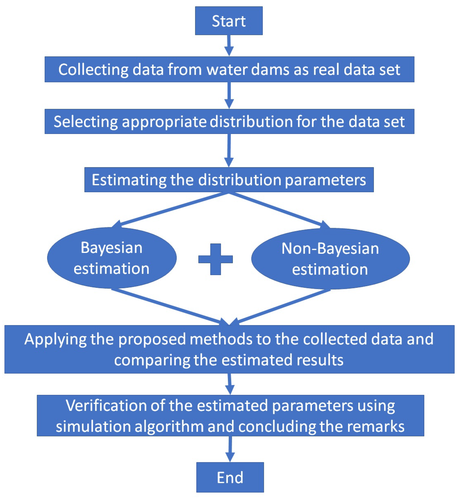
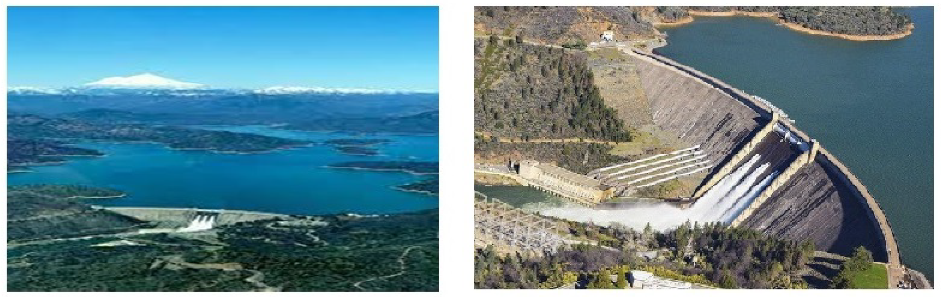
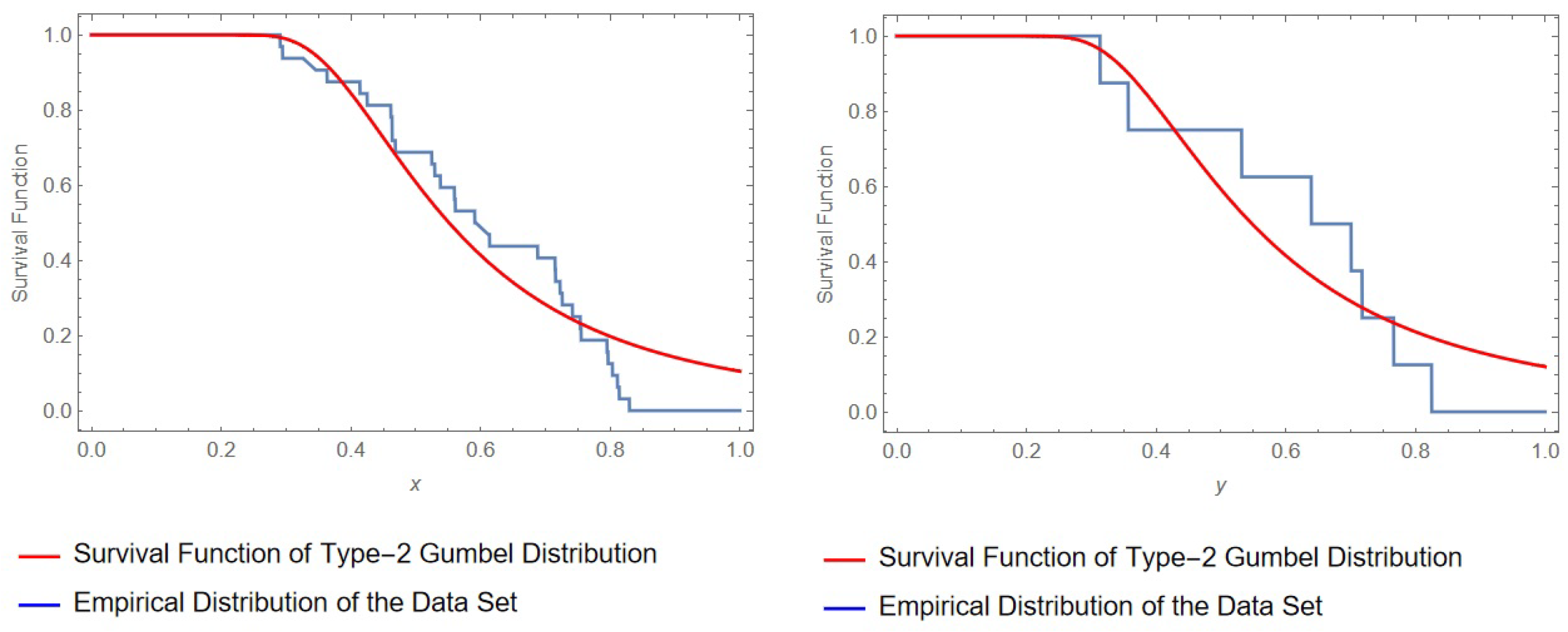
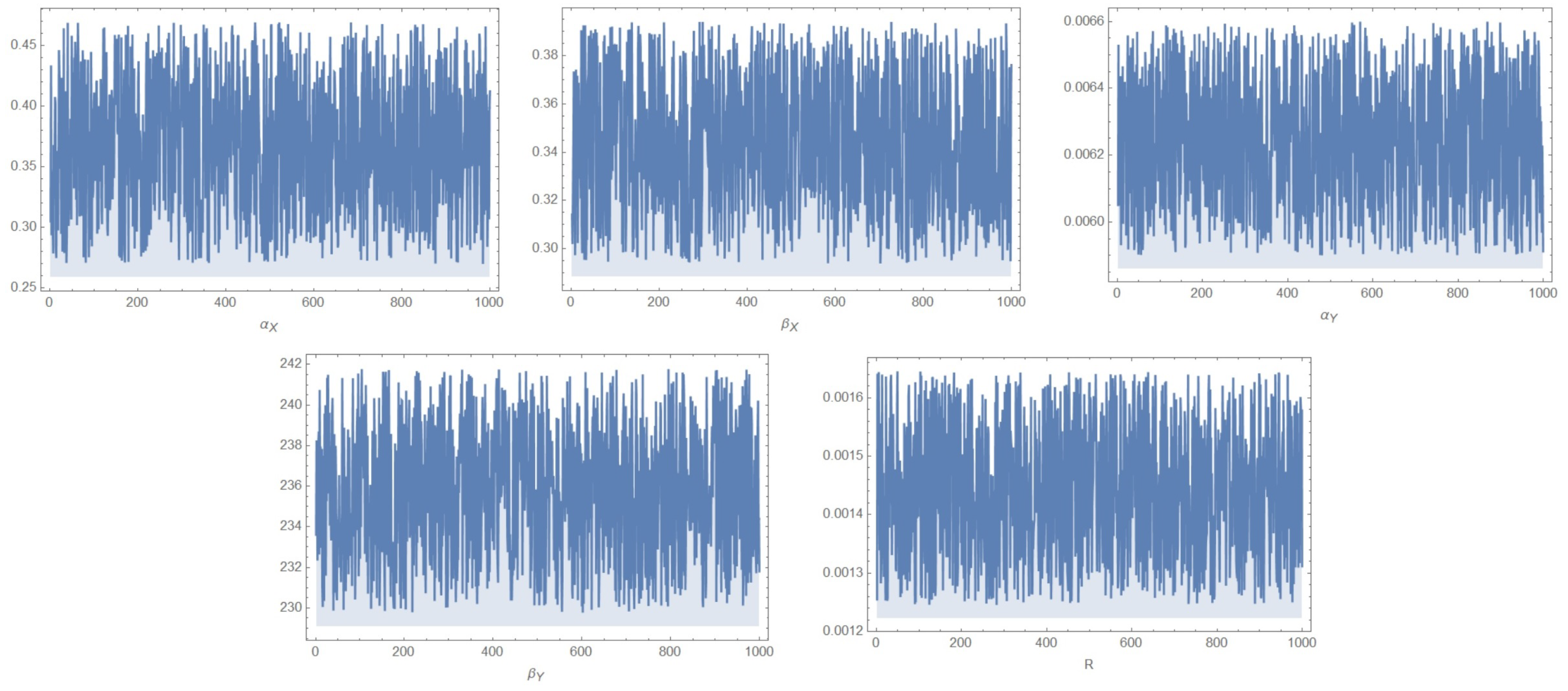
5. Real Data Analysis

In this section, the reliability function is estimated using the MLE and Bayesian estimation methods, where the data under consideration are obtained for the water capacity in the Shasta reservoir in the United States. The view of Shasta Lake during the season of floods in addition to a general view of the Shasta dam are shown in Figure 2.

To consider the scenario of the excessive drought, we will focus on the total amount of water in the period from 1980 until 2019. Our claim is that an excessive drought occurs if the total amount of water in August in two years of the next four years is less than the amount of water filling the reservoir in December of the preceding years, otherwise, no excessive drought will occur. This problem was previously studied in different contexts, i.e., see Fatma [19] and Akram [16]. The source of the data is available in [38].

For computational simplicity, the water amount in the reservoir for any given month is divided by the total capacity of the reservoir and the data will then be as follows:

$$X=\left(\begin{array}{cccc}0.5597& 0.8112& 0.8296& 0.7262\\ 0.7152& 0.4637& 0.3634& 0.4637\\ 0.2912& 0.4141& 0.7540& 0.5381\\ 0.7226& 0.5612& 0.8140& 0.7552\\ 0.5249& 0.6060& 0.7159& 0.5295\\ 0.7420& 0.4688& 0.3451& 0.4253\\ 0.7951& 0.6139& 0.4616& 0.2948\\ 0.6881& 0.7967& 0.5913& 0.8037\end{array}\right)\mathrm{and}Y=\left(\begin{array}{c}0.7009\\ 0.5321\\ 0.3572\\ 0.7179\\ 0.6395\\ 0.8279\\ 0.7665\\ 0.3135\end{array}\right)$$

The first row of the observations in matrix X represents the storage amount of water (divided by the total capacity storage of the lake) in August 1980–1983, respectively, while the second row represents this in August 1985–1988, respectively, and so on, with a sample size of 32 observations. Whereas the amount of water in December 1984, 1989, up to 2019 is represented by matrix Y, with a size of 8 observations. It was found that both X and Y values are well-fitted to the Gumbel Type II distribution. The Gumbel Type II distribution was chosen primarily because of its suitability for predicting the possibility of climatic events such as annual flood flows (which is the case of this study), earthquakes, and other natural disasters. However, fitting outcomes for certain classical models, such as the log-normal distribution, are poor, with p-values of $1.57936\times {10}^{-11}$ and $0.00194213$ for the X and Y datasets, respectively. While for the Gumbel Type II distribution, the Kolmogorov–Smirnov (KS) distance for X with the estimated parameters is $0.178521$ and the corresponding p-value is $0.230418$. Furthermore, for Y, the KS distance with the estimated parameters is $0.263293$ and the corresponding p-value is $0.550885$. A comparison between the empirical distribution of the dataset and the survival function of the Gumbel Type II distribution is presented in Figure 3.

For the complete dataset, the MLEs for the parameters, ${\alpha }_1$, ${\alpha }_2$, ${\beta }_1$, and ${\beta }_2$, and the reliability function, in addition to the Bayesian estimation with respect to SEL function are displayed in

Table 1. The point estimates for ${\alpha }_1$, ${\beta }_1$, ${\alpha }_2$, ${\beta }_2$ and R.

	${\mathit{\alpha }}_1$	${\mathit{\beta }}_1$	${\mathit{\alpha }}_2$	${\mathit{\beta }}_2$	${\mathit{R}}_{2,4}$
MLE	0.303858	0.402204	0.00569851	238.391	0.00789931
Bayes	0.469386	0.393857	0.00850074	237.782	0.00824543

.

From Table 1, the estimated values are relatively close to each other, which indicates the good performance of the estimators. In addition, the two estimators for the reliability function $R_{2,4}$ seem to be very close and approximately equal to zero, indicating no excessive droughts in these periods. The convergence for the estimated parameters using the MCMC method with 1000 iterations is shown in Figure 4.

6. Simulation Study

A Monte Carlo simulation analysis is carried out in this section comparing the performance of the MLE and Bayesian estimates of the distribution’s parameters ${\alpha }_1$, ${\beta }_1$, ${\alpha }_2$, and ${\beta }_2$ under various scenarios. The comparisons are made using the mean-squares-error (MSE) criterion. All computations are carried out in Mathematica 12, and all the results are obtained using 1000 Monte Carlo samples. We use various sample sizes (n) and $(s,k)$ values in the simulation setup. Various parameter values are selected with different sample sizes (n) such as $n=30,40,50,100$, and 150 and ${\alpha }_1$, ${\beta }_1$, ${\alpha }_2$, and ${\beta }_2$ are assumed to be (0.2, 0.5, 0.05, and 200) and (0.3, 0.4, 0.05, and 200), respectively.

Table 2. The MLE and Bayesian estimates for the parameters $({\alpha }_1,{\beta }_1,{\alpha }_2,{\beta }_2)=(0.2,0.5,0.05,200)$ with the associated MSE between parenthesis.

			MLE					Bayesian
$({\mathbf{\alpha }}_{\mathbf{1}},{\mathbf{\beta }}_{\mathbf{1}},{\mathbf{\alpha }}_{\mathbf{2}},{\mathbf{\beta }}_{\mathbf{2}})$	$(\mathit{s},\mathit{k})$	$\mathit{n}$	$\widehat{{\mathbf{\alpha }}_{\mathbf{1}}}$	$\widehat{{\mathbf{\beta }}_{\mathbf{1}}}$	$\widehat{{\mathbf{\alpha }}_{\mathbf{2}}}$	$\widehat{{\mathbf{\beta }}_{\mathbf{2}}}$		$\widehat{{\mathbf{\alpha }}_{\mathbf{1}}}$	$\widehat{{\mathbf{\beta }}_{\mathbf{1}}}$	$\widehat{{\mathbf{\alpha }}_{\mathbf{2}}}$	$\widehat{{\mathbf{\beta }}_{\mathbf{2}}}$
(0.2, 0.5, 0.05, 200)	(3, 5)	30	0.20146	0.50203	0.04999	199.837		0.1808	0.45054	0.04486	198.838
			(0.00017)	(0.00296)	(0.000)	(32.8054)		(0.0002)	(0.0034)	(0.000)	(33.0127)
		40	0.2014	0.50013	0.05001	199.969		0.18074	0.44884	0.04488	198.969
			(0.00013)	(0.00225)	(0.000)	(31.3774)		(0.00014)	(0.00271)	(0.000)	(33.9823)
		50	0.2011	0.50103	0.04998	199.897		0.18047	0.44964	0.04485	198.898
			(0.0001)	(0.00176)	(0.000)	(32.0521)		(0.00012)	(0.002)	(0.000)	(37.8047)
		100	0.20071	0.49831	0.04993	199.688		0.18012	0.4472	0.04481	198.689
			(0.00005)	(0.0009)	(0.000)	(31.9973)		(0.00005)	(0.00116)	(0.000)	(39.0693)
		150	0.20037	0.5002	0.04999	200.017		0.17982	0.4489	0.04486	199.017
			(0.00003)	(0.00059)	(0.000)	(33.7554)		(0.00004)	(0.00059)	(0.000)	(40.6417)
	(5, 5)	30	0.20222	0.49926	0.04997	199.657		0.18148	0.44805	0.04484	198.659
			(0.00017)	(0.00292)	(0.000)	(33.13)		(0.0002)	(0.00331)	(0.000)	(35.7178)
		40	0.20177	0.50036	0.04999	199.715		0.18107	0.44904	0.04486	198.716
			(0.00012)	(0.00205)	(0.000)	(32.5364)		(0.00013)	(0.00232)	(0.000)	(38.4116)
		50	0.20087	0.50181	0.04995	199.765		0.18027	0.45035	0.04483	198.767
			(0.0001)	(0.00176)	(0.000)	(34.8049)		(0.00012)	(0.00227)	(0.000)	(35.433)
		100	0.20051	0.5015	0.04999	199.824		0.17994	0.45006	0.04486	198.824
			(0.00005)	(0.00088)	(0.000)	(31.978)		(0.00005)	(0.00114)	(0.000)	(36.2068)
		150	0.20041	0.50021	0.05002	199.727		0.17986	0.44891	0.04489	198.728
			(0.00003)	(0.00058)	(0.000)	(32.943)		(0.00004)	(0.00058)	(0.000)	(34.9308)
	(5, 6)	30	0.20152	0.50146	0.05001	199.8		0.18085	0.45003	0.04488	198.801
			(0.00014)	(0.0022)	(0.000)	(32.295)		(0.00015)	(0.00232)	(0.000)	(33.4603)
		40	0.20155	0.50179	0.05005	199.89		0.18088	0.45032	0.04492	198.891
			(0.00011)	(0.0018)	(0.000)	(34.2618)		(0.00013)	(0.00204)	(0.000)	(34.2076)
		50	0.20141	0.49875	0.05	199.765		0.18075	0.44759	0.04487	198.766
			(0.00009)	(0.00149)	(0.000)	(30.8775)		(0.0001)	(0.00175)	(0.000)	(32.8875)
		100	0.20038	0.5005	0.04995	200.074		0.17983	0.44916	0.04483	199.074
			(0.00004)	(0.00067)	(0.000)	(31.4818)		(0.00005)	(0.00075)	(0.000)	(32.6242)
		150	0.20014	0.50009	0.04999	200.067		0.17962	0.4488	0.04486	199.067
			(0.00003)	(0.00052)	(0.000)	(33.1109)		(0.00004)	(0.00064)	(0.000)	(36.4121)

and

Table 3. The MLE and Bayesian estimates for the parameters $({\alpha }_1,{\beta }_1,{\alpha }_2,{\beta }_2)=(0.3,0.4,0.05,200)$ with the associated MSE between parenthesis.

			MLE					Bayesian
$({\mathbf{\alpha }}_{\mathbf{1}},{\mathbf{\beta }}_{\mathbf{1}},{\mathbf{\alpha }}_{\mathbf{2}},{\mathbf{\beta }}_{\mathbf{2}})$	$(\mathit{s},\mathit{k})$	$\mathit{n}$	$\widehat{{\mathbf{\alpha }}_{\mathbf{1}}}$	$\widehat{{\mathbf{\beta }}_{\mathbf{1}}}$	$\widehat{{\mathbf{\alpha }}_{\mathbf{2}}}$	$\widehat{{\mathbf{\beta }}_{\mathbf{2}}}$		$\widehat{{\mathbf{\alpha }}_{\mathbf{1}}}$	$\widehat{{\mathbf{\beta }}_{\mathbf{1}}}$	$\widehat{{\mathbf{\alpha }}_{\mathbf{2}}}$	$\widehat{{\mathbf{\beta }}_{\mathbf{2}}}$
(0.3, 0.4, 0.05, 200)	(3, 5)	30	0.3025	0.39763	0.05	199.822		0.27147	0.35685	0.04487	198.822
			(0.00036)	(0.00226)	(0.000)	(33.8999)		(0.00038)	(0.00234)	(0.000)	(40.3491)
		40	0.30229	0.39954	0.04984	199.835		0.27129	0.35856	0.04473	198.836
			(0.00026)	(0.0016)	(0.000)	(34.5172)		(0.00026)	(0.00166)	(0.000)	(35.5571)
		50	0.30102	0.40185	0.05003	199.753		0.27014	0.36064	0.0449	198.754
			(0.00021)	(0.00123)	(0.000)	(34.6565)		(0.00025)	(0.00138)	(0.000)	(42.4399)
		100	0.30021	0.40196	0.05007	200.059		0.26942	0.36074	0.04493	199.059
			(0.00012)	(0.0007)	(0.000)	(32.4818)		(0.00013)	(0.0007)	(0.000)	(32.5149)
		150	0.30078	0.39987	0.04999	199.555		0.26993	0.35886	0.04486	198.558
			(0.00007)	(0.00043)	(0.000)	(33.0983)		(0.00009)	(0.00052)	(0.000)	(38.4439)
	(5, 5)	30	0.30285	0.4029	0.04994	199.654		0.27179	0.36157	0.04482	198.656
			(0.00038)	(0.00225)	(0.000)	(33.433)		(0.00049)	(0.00238)	(0.000)	(40.4265)
		40	0.30167	0.40134	0.04994	200.091		0.27073	0.36017	0.04482	199.09
			(0.00026)	(0.00166)	(0.000)	(34.0351)		(0.00032)	(0.00196)	(0.000)	(33.7554)
		50	0.30159	0.40057	0.04993	200.15		0.27065	0.35949	0.04481	199.149
			(0.00022)	(0.00129)	(0.000)	(34.2804)		(0.00026)	(0.00164)	(0.000)	(43.0006)
		100	0.30051	0.40013	0.04995	199.983		0.26969	0.35909	0.04483	198.983
			(0.00011)	(0.00068)	(0.000)	(32.9482)		(0.00011)	(0.00069)	(0.000)	(33.3591)
		150	0.30005	0.40084	0.04996	199.626		0.26928	0.35973	0.04484	198.628
			(0.00007)	(0.00044)	(0.000)	(33.8825)		(0.00008)	(0.00051)	(0.000)	(35.5814)
	(5, 6)	30	0.30217	0.40028	0.04992	200.064		0.27118	0.35923	0.0448	199.063
			(0.00031)	(0.00158)	(0.000)	(33.822)		(0.0004)	(0.00236)	(0.000)	(36.4273)
		40	0.30233	0.39868	0.05001	199.671		0.27132	0.35779	0.04488	198.672
			(0.00025)	(0.00129)	(0.000)	(32.1462)		(0.0003)	(0.00168)	(0.000)	(37.4052)
		50	0.30195	0.39879	0.05	200.079		0.27098	0.35789	0.04487	199.079
			(0.0002)	(0.00109)	(0.000)	(33.8499)		(0.00021)	(0.00116)	(0.000)	(40.087)
		100	0.30038	0.40072	0.05001	199.938		0.26957	0.35962	0.04489	198.938
			(0.00009)	(0.00055)	(0.000)	(32.5754)		(0.00011)	(0.00064)	(0.000)	(36.7374)
		150	0.30054	0.40001	0.04998	200.075		0.26971	0.35899	0.04486	199.075
			(0.00006)	(0.00036)	(0.000)	(33.7145)		(0.00006)	(0.0004)	(0.000)	(38.2541)

show that in most cases, the Bayesian estimators of the parameters have a large bias compared with the MLEs for small sample sizes. However, when the sample sizes grow larger, all of the estimators exhibit small biases. In terms of the MSE criterion, it is clear that as the sample size increases, the MSEs for the estimates of ${\alpha }_1$, ${\beta }_1$, and ${\alpha }_2$ decrease, as expected. However, it was noticed that the MSE for ${\beta }_2$ does not decrease as the sample size increases; hence, sometimes some values of MSE violate this pattern due to some causes such as the numerical solution of a certain number of non-linear simultaneous equations. It should be noted that informative priors improve the performance of Bayesian estimates in a reasonable way. As sample sizes grow larger, the MSE values for all estimators become nearly identical. To emphasize the performance of the proposed methods, another criterion is applied which is the coverage probability. The coverage probability indicates how many times a confidence interval contains the initial value of the estimated parameters through the number of simulated samples. In addition, the average interval lengths for both the ACIs and CRIs are calculated and tabulated in

Table 4. ACIs and CRIs for $({\alpha }_1,{\beta }_1,{\alpha }_2,{\beta }_2)=(0.2,0.5,0.05,200)$ with their corresponding coverage probabilities between parenthesis.

			MLE					Bayesian
$({\mathbf{\alpha }}_{\mathbf{1}},{\mathbf{\beta }}_{\mathbf{1}},{\mathbf{\alpha }}_{\mathbf{2}},{\mathbf{\beta }}_{\mathbf{2}})$	$(\mathit{s},\mathit{k})$	$\mathit{n}$	$\widehat{{\mathbf{\alpha }}_{\mathbf{1}}}$	$\widehat{{\mathbf{\beta }}_{\mathbf{1}}}$	$\widehat{{\mathbf{\alpha }}_{\mathbf{2}}}$	$\widehat{{\mathbf{\beta }}_{\mathbf{2}}}$		$\widehat{{\mathbf{\alpha }}_{\mathbf{1}}}$	$\widehat{{\mathbf{\beta }}_{\mathbf{1}}}$	$\widehat{{\mathbf{\alpha }}_{\mathbf{2}}}$	$\widehat{{\mathbf{\beta }}_{\mathbf{2}}}$
(0.2, 0.5, 0.05, 200)	(3, 5)	30	0.0507	0.2109	0.0281	567.508		0.0304	0.1265	0.0169	29.5104
			(0.95)	(0.951)	(1.000)	(1.000)		(0.9949)	(0.9951)	(0.995)	(0.995)
		40	0.0436	0.1833	0.0244	491.674		0.0261	0.11	0.0146	25.567
			(0.944)	(0.944)	(1.000)	(1.000)		(0.995)	(0.995)	(0.995)	(0.9949)
		50	0.0389	0.1643	0.0218	438.494		0.0233	0.0986	0.0131	22.8017
			(0.951)	(0.948)	(1.000)	(1.000)		(0.9951)	(0.9951)	(0.9951)	(0.9949)
		100	0.0275	0.1159	0.0153	308.949		0.0165	0.0695	0.0092	16.0653
			(0.954)	(0.935)	(1.000)	(1.000)		(0.9949)	(0.995)	(0.9949)	(0.995)
		150	0.0224	0.0948	0.0125	252.359		0.0134	0.0569	0.0075	13.1227
			(0.962)	(0.948)	(1.000)	(1.000)		(0.9949)	(0.9951)	(0.9949)	(0.995)
	(5, 5)	30	0.0506	0.2115	0.0283	570.071		0.0303	0.1269	0.017	29.6437
			(0.951)	(0.933)	(1.000)	(1.000)		(0.9949)	(0.995)	(0.9952)	(0.9949)
		40	0.0435	0.1839	0.0245	492.382		0.0261	0.1103	0.0147	25.6038
			(0.949)	(0.945)	(1.000)	(1.000)		(0.9949)	(0.9949)	(0.995)	(0.995)
		50	0.039	0.164	0.0218	439.355		0.0234	0.0984	0.0131	22.8464
			(0.964)	(0.956)	(1.000)	(1.000)		(0.995)	(0.9951)	(0.9949)	(0.9951)
		100	0.0274	0.1165	0.0154	309.768		0.0164	0.0699	0.0092	16.1079
			(0.954)	(0.941)	(1.000)	(1.000)		(0.995)	(0.995)	(0.9951)	(0.995)
		150	0.0224	0.0949	0.0125	252.428		0.0134	0.057	0.0075	13.1262
			(0.953)	(0.952)	(1.000)	(1.000)		(0.9951)	(0.9951)	(0.9951)	(0.995)
	(5, 6)	30	0.046	0.1931	0.0282	567.143		0.0276	0.1159	0.0169	29.4914
			(0.946)	(0.951)	(1.000)	(1.000)		(0.9951)	(0.995)	(0.995)	(0.995)
		40	0.0397	0.168	0.0245	493.172		0.0238	0.1008	0.0147	25.6449
			(0.945)	(0.951)	(1.000)	(1.000)		(0.9949)	(0.9952)	(0.995)	(0.995)
		50	0.0356	0.1499	0.0218	439.107		0.0213	0.09	0.0131	22.8335
			(0.938)	(0.941)	(1.000)	(1.000)		(0.9949)	(0.995)	(0.9951)	(0.9948)
		100	0.025	0.106	0.0153	308.724		0.015	0.0636	0.0092	16.0537
			(0.957)	(0.958)	(1.000)	(1.000)		(0.9951)	(0.9951)	(0.9949)	(0.9949)
		150	0.0204	0.0866	0.0125	251.642		0.0123	0.052	0.0075	13.0854
			(0.955)	(0.941)	(1.000)	(1.000)		(0.9949)	(0.9951)	(0.995)	(0.995)

and

Table 5. ACIs and CRIs for $({\alpha }_1,{\beta }_1,{\alpha }_2,{\beta }_2)=(0.3,0.4,0.05,200)$ with their corresponding coverage probabilities between parenthesis.

			MLE					Bayesian
$({\mathbf{\alpha }}_{\mathbf{1}},{\mathbf{\beta }}_{\mathbf{1}},{\mathbf{\alpha }}_{\mathbf{2}},{\mathbf{\beta }}_{\mathbf{2}})$	$(\mathit{s},\mathit{k})$	$\mathit{n}$	$\widehat{{\mathbf{\alpha }}_{\mathbf{1}}}$	$\widehat{{\mathbf{\beta }}_{\mathbf{1}}}$	$\widehat{{\mathbf{\alpha }}_{\mathbf{2}}}$	$\widehat{{\mathbf{\beta }}_{\mathbf{2}}}$		$\widehat{{\mathbf{\alpha }}_{\mathbf{1}}}$	$\widehat{{\mathbf{\beta }}_{\mathbf{1}}}$	$\widehat{{\mathbf{\alpha }}_{\mathbf{2}}}$	$\widehat{{\mathbf{\beta }}_{\mathbf{2}}}$
(0.3, 0.4, 0.05, 200)	(3, 5)	30	0.0759	0.1848	0.0283	571.737		0.0455	0.1109	0.017	29.7303
			(0.952)	(0.938)	(1.000)	(1.000)		(0.9951)	(0.995)	(0.995)	(0.995)
		40	0.0656	0.1594	0.0244	492.21		0.0394	0.0957	0.0147	25.5949
			(0.959)	(0.949)	(1.000)	(1.000)		(0.995)	(0.995)	(0.9951)	(0.9949)
		50	0.0582	0.1438	0.0217	437.88		0.0349	0.0863	0.013	22.7697
			(0.954)	(0.953)	(1.000)	(1.000)		(0.9948)	(0.9948)	(0.9951)	(0.995)
		100	0.0412	0.1013	0.0154	309.34		0.0247	0.0608	0.0092	16.0857
			(0.96)	(0.95)	(1.000)	(1.000)		(0.995)	(0.9951)	(0.9949)	(0.995)
		150	0.0335	0.0827	0.0125	251.705		0.0201	0.0496	0.0075	13.0887
			(0.946)	(0.946)	(1.000)	(1.000)		(0.995)	(0.995)	(0.995)	(0.9949)
	(5, 5)	30	0.0759	0.1844	0.0282	568.27		0.0456	0.1106	0.0169	29.55
			(0.94)	(0.95)	(1.000)	(1.000)		(0.995)	(0.995)	(0.9951)	(0.9952)
		40	0.0655	0.1599	0.0245	493.459		0.0393	0.0959	0.0147	25.6599
			(0.95)	(0.942)	(1.000)	(1.000)		(0.9951)	(0.9948)	(0.995)	(0.995)
		50	0.0584	0.1429	0.0218	438.597		0.035	0.0857	0.0131	22.807
			(0.947)	(0.94)	(1.000)	(1.000)		(0.9951)	(0.9951)	(0.9949)	(0.9949)
		100	0.0411	0.1015	0.0153	309.374		0.0247	0.0609	0.0092	16.0874
			(0.954)	(0.95)	(1.000)	(1.000)		(0.995)	(0.9951)	(0.9951)	(0.995)
		150	0.0336	0.0827	0.0125	252.025		0.0201	0.0496	0.0075	13.1053
			(0.953)	(0.964)	(1.000)	(1.000)		(0.9952)	(0.9951)	(0.995)	(0.9949)
	(5, 6)	30	0.0689	0.1689	0.0283	570.784		0.0413	0.1014	0.017	29.6808
			(0.956)	(0.945)	(1.000)	(1.000)		(0.995)	(0.9951)	(0.995)	(0.9951)
		40	0.0597	0.1463	0.0245	494.035		0.0358	0.0878	0.0147	25.6898
			(0.953)	(0.948)	(1.000)	(1.000)		(0.995)	(0.9951)	(0.995)	(0.995)
		50	0.0533	0.1305	0.0217	437.669		0.032	0.0783	0.013	22.7588
			(0.944)	(0.945)	(1.000)	(1.000)		(0.9951)	(0.995)	(0.995)	(0.9953)
		100	0.0376	0.0925	0.0153	308.903		0.0225	0.0555	0.0092	16.063
			(0.949)	(0.954)	(1.000)	(1.000)		(0.9951)	(0.9951)	(0.995)	(0.9949)
		150	0.0306	0.0756	0.0125	252.177		0.0184	0.0453	0.0075	13.1132
			(0.957)	(0.952)	(1.000)	(1.000)		(0.9951)	(0.9947)	(0.995)	(0.995)

. It is noted that for various values of ${\alpha }_1$, ${\beta }_1$, ${\alpha }_2$, and ${\beta }_2$, for n, s, and k, the CRIs perform better than the ACIs through the coverage probability and the average lengths of intervals.

7. Conclusions

In this study, the stress–strength model describing the amount of water held in a certain reservoir over time is modeled parametrically using the Gumbel Type II distribution. It introduces a mathematical procedure for obtaining a closed form for R. In addition to the Bayesian technique, the maximum likelihood estimation for the parameter R is carried out. A simulation study is conducted to compare the effectiveness of the various approaches. The analysis revealed that the water in storage is sufficiently durable. In other words, since the value of R is constantly close to zero, droughts are unlikely to occur even when this amount of water is subjected to evaporation and consumption.

References

1. Birnbaum, Z.W. On a use of Mann–Whitney statistics. Proc. Third Berkley Symp. Math. Stat. Probab. 1956, 1, 13–17. [Google Scholar]
2. Hanagal, D.D. Estimation of system reliability. Stat. Pap. 1999, 40, 99–106. [Google Scholar] [CrossRef]
3. Kotz, S.; Lumelskii, Y.; Pensky, M. The Stress-Strength Model and Its Generalization: Theory and Applications; World Scientific Publishing Company: Singapore, 2003. [Google Scholar]
4. Raqab, M.Z.; Madi, M.T.; Kundu, D. Estimation of R = P(Y < X) for the 3-parameter generalized exponential distribution. Commun. Stat. 2008, 37, 2854–2864. [Google Scholar]
5. Kundu, D.; Raqab, M.Z. Estimation of R = P(Y < X) for three parameter Weibull distribution. Stat. Probab. Lett. 2009, 79, 1839–1846. [Google Scholar]
6. Lio, Y.L.; Tsai, T.R. Estimation of δ = P(X < Y) for Burr XII distribution based on the progressively first failure-censored samples. J. Appl. Stat. 2012, 39, 309–322. [Google Scholar]
7. Nadar, M.; Kizilaslan, F.; Papadopoulos, A. Classical and Bayesian estimation of P(Y < X) for Kumaraswamy’s distribution. J. Stat. Comput. Simul. 2014, 84, 1505–1529. [Google Scholar]
8. Rao, G.S.; Kantam, R.R.L. Estimation of reliability in multi-component stress-strength model: Log-logistic distribution. Electron. J. Appl. Stat. Anal. 2010, 3, 75–84. [Google Scholar]
9. Rao, G.S. Estimation of reliability in multi-component stress-strength model based on Rayleigh distribution. Prob. Stat. Forum. 2012, 5, 155–161. [Google Scholar]
10. Rao, G.S. Estimation of reliability in multi-component stress-strength model based on inverse exponential distribution. Int. J. Stat. Econ. 2013, 10, 28–37. [Google Scholar]
11. Rao, G.S.; Kantam, R.R.L.; Rosaiah, K.; Reddy, J.P. Estimation of reliability in multi-component stress-strength model based on inverse Rayleigh distribution. J. Stat. Appl. Probab. 2013, 2, 261–267. [Google Scholar] [CrossRef]
12. Kizilaslan, F.; Nadar, M. Estimation of reliability in a multi-component stress-strength model based on a bivariate Kumaraswamy distribution. Stat. Pap. 2018, 59, 307–340. [Google Scholar] [CrossRef]
13. Nadar, M.; Kizilaslan, F. Estimation of reliability in a multi-component stress-strength model based on a Marshall–Olkin bivariate weibull Distribution. IEEE Trans. Reliab. 2016, 65, 370–380. [Google Scholar] [CrossRef]
14. Dey, S.; Singh, S.; Tripathi, Y.M.; Asgharzadeh, A. Estimation and prediction for a progressively censored generalized inverted exponential distribution. Stat. Methodol. 2016, 32, 185–202. [Google Scholar] [CrossRef]
15. Wu, X.Z. Implementing statistical fitting and reliability analysis for geotechnical engineering problems in R. Georisk Assess. Manag. Risk Eng. Syst. Geohazards 2017, 11, 173–188. [Google Scholar] [CrossRef]
16. Kohansal, A. On estimation of reliability in a multi-component stress-strength model for a Kumaraswamy distribution based on progressively censored sample. Stat. Pap. 2019, 60, 2185–2224. [Google Scholar] [CrossRef]
17. Xu, J.; Dang, C. A novel fractional moments-based maximum entropy method for high-dimensional reliability analysis. Appl. Math. Model. 2019, 75, 749–768. [Google Scholar] [CrossRef]
18. Zhang, X.; Low, Y.M.; Koh, C.G. Maximum entropy distribution with fractional moments for reliability analysis. Struct. Saf. 2020, 83, 101904. [Google Scholar] [CrossRef]
19. Akgul, F. Classical and Bayesian estimation of multi-component stress-strength reliability for exponentiated Pareto distribution. Soft Comput. 2021, 25, 9185–9197. [Google Scholar] [CrossRef]
20. Wang, Z.Z.; Goh, S.H. A maximum entropy method using fractional moments and deep learning for geotechnical reliability analysis. Acta Geotech. 2022, 17, 1147–1166. [Google Scholar] [CrossRef]
21. Wang, Z.Z.; Jiang, S.H. Characterizing geotechnical site investigation data: A comparative study using a novel distribution model. Acta Geotech. 2022. [Google Scholar] [CrossRef]
22. Ahmad, H.H.; Almetwally, E.M.; Ramadan, D.A. A comparative inference on reliability estimation for a multi-component stress-strength model under power Lomax distribution with applications. AIMS Math. 2022, 7, 18050–18079. [Google Scholar] [CrossRef]
23. Johari, A.; Vali, B.; Golkarfard, H. System reliability analysis of ground response based on peak ground acceleration considering soil layers cross-correlation. Soil Dyn. Earthq. Eng. 2021, 141, 106475. [Google Scholar] [CrossRef]
24. Johari, A.; Rahmati, H. System reliability analysis of slopes based on the method of slices using sequential compounding method. Comput. Geotech. 2019, 114, 103116. [Google Scholar] [CrossRef]
25. Johari, A.; Hajivand, A.K.; Binesh, S. System reliability analysis of soil nail wall using random finite element method. Bull. Eng. Geol. Environ. 2020, 79, 2777–2798. [Google Scholar] [CrossRef]
26. Abbas, K.; Fu, J.; Tang, Y. Bayesian Estimation of Gumbel Type-II Distribution. Data Sci. J. 2013, 12, 33–46. [Google Scholar] [CrossRef] [Green Version]
27. Kotz, S.; Nadarajah, S. Extreme Value Distributions: Theory and Applications; Imperial College Press: London, UK, 2000. [Google Scholar]
28. Nadarajah, S.; Kotz, S. The exponentiated type distributions. Acta Appl. Math. 2006, 92, 97–111. [Google Scholar] [CrossRef]
29. Feroze, N.; Muahmmad, A. Bayesian Analysis of Gumbel Type II Distribution under Censored Data, 1st ed.; LAP LAMBERT Academic Publishing: Saarbruecken, Germany, 2014. [Google Scholar]
30. Mansour, M.M.; Aboshady, M.S. Assessing The Performance of Insulating Fluids Via Point of Statistical Inference View. TWMS J. App. Eng. Math. 2022, 12, 469–480. [Google Scholar]
31. Bhattacharyya, G.K.; Johnson, R.A. Estimation of reliability in a multi-component stress-strength model. J. Am. Stat. Assoc. 1974, 69, 966–970. [Google Scholar] [CrossRef]
32. Azzalini, A. Statistical Inference Based on the Likelihood, 1st ed.; Chapman and Hall/CRC: London, UK, 1996. [Google Scholar]
33. Louis, T.A. Finding the observed information matrix when using the EM algorithm. J. R. Statist. Soc. B 1982, 44, 226–233. [Google Scholar]
34. Lawless, J.F. Statistical Models and Methods for Lifetime Data, 2nd ed.; Wiley-Interscience: New York, NY, USA, 2002. [Google Scholar]
35. Kundu, D.; Howlader, H. Bayesian inference and prediction of the inverse Weibull distribution for Type-II censored data. Comput. Stat. Data Anal. 2010, 54, 1547–1558. [Google Scholar] [CrossRef]
36. Dey, S.; Dey, T. On progressively censored generalized inverted exponential distribution. J. Appl. Stat. 2014, 41, 2557–2576. [Google Scholar] [CrossRef]
37. Metropolis, N.; Rosenbluth, A.W.; Rosenbluth, M.N.; Teller, A.H. Equations of state calculations by fast computing machines. J. Chem. Phys. 1953, 21, 1087–1092. [Google Scholar] [CrossRef] [Green Version]
38. Available online: https://cdec.water.ca.gov/dynamicapp/QueryMonthly?s=SHA&end=1986-10&span=5years (accessed on 1 July 2021).
Figure 1. A flowchart indicating the research process.
Symmetry 15 00766 g001
Figure 2. View of Shasta Lake during the season of floods and a plan view for the dam.
Symmetry 15 00766 g002
Figure 3. Empirical and fitted survival functions for the two datasets X and Y.
Symmetry 15 00766 g003
Figure 4. Convergence for the estimated parameters α 1 , β 1 , α 1 , β 2 and R.
Symmetry 15 00766 g004