
A Numerical Solution of Symmetric Angle Ply Plates Using Higher-Order Shear Deformation Theory


Department of Mathematics and Statistics, College of Science, King Faisal University, P.O. Box 400, Al Ahsa 31982, Saudi Arabia
Symmetry 2023, 15(3), 767; https://doi.org/10.3390/sym15030767
Submission received: 24 February 2023
/
Revised: 11 March 2023
/
Accepted: 17 March 2023
/
Published: 21 March 2023
(This article belongs to the Special Issue Symmetry and Approximation Methods II)
Abstract
:This research aims to provide the numerical analysis solution of symmetric angle ply plates using higher-order shear deformation theory (HSDT). The vibration of symmetric angle ply composite plates is analyzed using differential equations consisting of supplanting and turning functions. These supplanting and turning functions are numerically approximated through spline approximation. The obtained global eigenvalue problem is solved numerically to find the eigenfrequency parameter and a related eigenvector of spline coefficients. The plates of different constituent components are used to study the parametric effects of the plate’s aspect ratio, side-to-thickness ratio, assembling sequence, number of composite layers, and alignment of each layer on the frequency of the plate. The obtained results are validated by existing literature.
1. Introduction
The research aims to provide a numerical analysis solution for symmetric angle ply plates using HSDT. The vibration of symmetric angle ply composite plates is analyzed using supplanting and turning functions, which are numerically approximated by spline approximation. Laminated plates have widely been used in many engineering fields and engineering structures because of their ability to alter mechanical properties. Additionally, the composite plates offer higher stiffness-to-weight ratios, strength-to-weight ratios, and shock-absorbing features than the homogeneous plates. One of the benefits of using composite plates leads to designing such structures which have maximum reliability and minimum weight. Layered plates show larger thickness effects than plates made of homogeneous materials, which tend to study the free vibration of laminated composite plates under third-order shear deformation theory.
The classical theory (CT) is based on the Love–Kirchhoff assumption. In this theory, the lines which are normal to the undeformed and deformed mid-plane remain straight and normal and do not experience any stretching along the z direction. The stress of thin composite plates can be precisely calculated by CT. However, it is not appropriate for thick laminated plates because the natural frequencies are overestimated (Vinson [1]; Noor and Burton [2]). So, in order to study relatively thick plates, the effect of shear deformation should be taken into account. Yang, Nooris, and Stavsky [3] developed the first-order shear deformation theory (FSDT) which states that there is constant shear strain through the z direction of the plate (transverse shear strain). Moreover, there are different higher-order plate theories to precisely calculate the transverse shear stresses which effectively occurs in thick plates. In higher-order plate theories, the displacements are extended to any desired degree in terms of thickness coordinates (Vinson [1] Noor and Burton [2]). In third-order plate theory, the displacement functions are extended to the terms with the power of three in thickness coordinates to have a quadratic variation of transverse shear strains and transverse shear stresses through the plate thickness. This avoids the need for a shear correction coefficient (Reddy [4]). The third-order plate TSDT theory by Reddy is widely used because it can represent transverse shear stresses in an efficient way.
Ghiamy and Amoushahi [5] investigated the stability of sandwich plates using the third-order shear deformation theory. Free and forced vibrations of graphene-filled plates were analyzed by Parida and Jena [6]. Zhao et al. [7] used the Jacobi–Ritz approach to study annular plates based on a higher-order shear deformation theory. Tian et al. [8] studied the nonlinear stability of organic solar cells using the third-order shear deformation plate theory. Bending, free vibration, and buckling of FGM plates were analyzed under HSDT by Belkhodja [9]. Third-order shear deformation theory was analyzed on graphene nanoplates for the modified couple stress theory (Eskandari et al. [10]). Shi and Dong [11] used the refined hyperbolic shear deformation theory to analyze the laminated composite plates. Javani et al. [12] used the GDQE procedure to study the free vibration of FG-GPLRC folded plates. A new higher-order shear deformation theory was used to study the free vibration of sandwich-curved beams (Sayyad and Avhad [13]). Ellali et al. [14] investigated the thermal buckling of a sandwich beam attached to piezoelectric layers based on the shear deformation theory. Bending, free vibration, and buckling analysis of functionally graded porous beams were examined using the shear deformation theory by Nguyen et al. [15]. Peng et al. [16] used the MK method to study static and free vibration analysis of stiffened FGM plates. Free vibration of functionally graded porous non-uniform thickness annular nanoplates using the ES-MITC3 element was studied by Pham et al. [17]. Hung et al. [18] used the modified strain gradient theory to analyze refined isogeometric plates. Sharma et al. [19] investigated the static and free vibration of smart variable stiffness laminated composite plates. Cho [20] examined the nonlinear free vibration of functionally graded CNT-reinforced plates. Functionally graded plates were studied for their static and free vibration by Zang et al. [21]. Ghosh and Haldar [22] analyzed the free vibration of laminated composite plates on elastic point supports using the finite element method. The extended Ritz method was used to analyze the free vibrations of cracked variable stiffness composite plates by Milazzo [23]. Saiah et al. [24] studied the free vibration behavior of nanocomposite laminated plates containing functionally graded graphene-reinforced composite plies. Singh and Karathanasopoulos [25] examined the composite plates using an elasticity solution under the patch loads. Belardi et al. [26] investigated the Ritz method to analyze the bending and stress of sector plates. Zhong et al. [27] analyzed the laminated annular plate backed by double cylindrical acoustic cavities.
Several studies have been conducted to investigate the mechanical properties and behavior of composite materials, including alkali-activated composites (Wang et al. [28]), hierarchical cellular honeycombs (Zhang et al. [29]), welding residual stress distribution of corrugated steel webs (Zhang et al. [30]), and microcracking behavior of crystalline rock (Peng et al. [31]). However, to the best of our knowledge, there are limited studies that have investigated the parametric effects of the plate’s aspect ratio, side-to-thickness ratio, assembling sequence, number of composite layers, and alignment of each layer on the frequency of symmetric angle ply plates.
This research utilizes differential equations in terms of displacement and rotational functions to analyze the vibration of symmetric angle ply composite plates. The spline approximation method is used to numerically approximate the displacement and rotational functions. The obtained spline coefficients are then used to solve a generalized eigenvalue problem numerically. The eigenvalue problem provides an eigenfrequency parameter and an associated eigenvector, which can be used to study the frequency response of the plate. The simply supported boundary condition is considered to analyze the geometric effects of the plate’s aspect ratio, side-to-thickness ratio, assembling sequence, number of composite layers, and alignment of each layer on the frequency of the plate. Results are narrated by using graphs and tables.
2. Solution of Problem
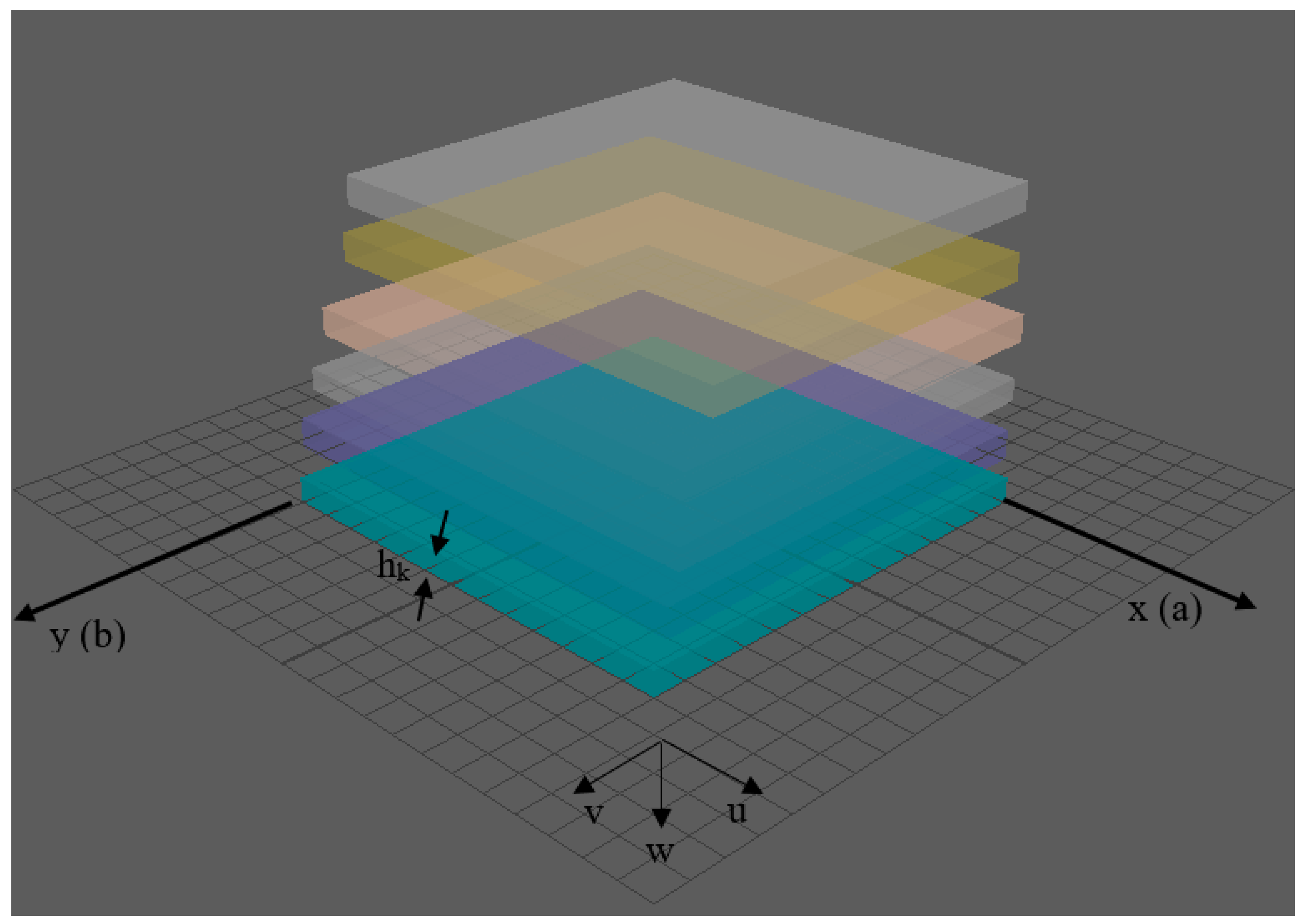
A rectangular plate considered has the Cartesian coordinate system , and , with the plane placed at mid-depth (reference surface) of the plate and taken normal to the plate, as shown in Figure 1. Here, and are the lengths of the sides of the plate along the and directions, respectively, is the total thickness, and is the thickness of the k-th layer of the plate.
The following equilibrium equations are derived using the dynamic version of the principle of virtual displacements for the higher-order theory (Reddy [32]).
Equation (1) is an equilibrium equation in the dynamic form as it consists of force, moment, transverse shear force resultants, and inertia force components.
are mass moments of inertia, which are defined as follows:
and is the material density of the -th layer. , and are the displacement components in the , and directions, respectively, , , and are the in-plane displacements of the middle plane, and and are the shear rotations of any point on the middle surface of the plate.
where , , and are in-plane force resultant, moment resultant, and transverse shear force resultants, respectively. and denote higher-order stress resultants.
The stress resultants are defined as:
The stress–strain relationships for the k-th layer, after neglecting transverse normal strain and stress, is of the form:
where are elements of the stiffness matrix defined in Appendix A.
When the materials are oriented at an angle with the -axis, the transformed stress–strain relationships are as follows:
where are elements of the transformed stiffness matrix given in Appendix A.
In-plane strains are defined as:
where:
The shear strain components are defined as:
where:
When any structure vibrates with a certain frequency, it causes stress and in return strain. Strain is the ratio of the change in length to the original length. Deformations that are applied perpendicular to the cross-section are normal strains , while deformations applied parallel to the cross-section are shear strains .
The stress–strain relationships are obtained as follows:
where , , , , and are obtained by integrating stress and strain components across the thickness of the plate. After integration, a modified equation in matrix form is written as Equation (7). Values of strain and shear strain component given in Equations (2)–(4) are inserted to the given system of the equation. After that, displacements and rotational functions given in Equation (9) are used and the resulting Equation (10) is obtained.
Stiffness coefficients are defined as:
for .
Where the elastic coefficients and (extensional and bending stiffnesses) and and are the higher-order stiffness coefficients.
The supplanting and turning functions are assumed in the separable form for symmetric angle ply plates as cos and sine functions as follows:
The non-dimensional parameters introduced are as follows:
is the frequency parameter and is the relative layer thickness of the k-th layer.
is the aspect ratio, is the distance co-ordinate, and is the side-to-thickness ratio.
Using cos and sine functions for displacements and rotational functions modified differential equations, which are obtained as follows:
where
Method of Solution
Equation (10) contains derivatives of supplanting and turning functions. Spline approximation is used to approximate these functions, with X having a range between [0, 1]. The purpose of using splines for approximation is for their high precision and rapid rate of convergence (Schoenberg and Witney [33]).
The spline approximation defines the supplanting , and the turning functions as follows:
Here, is the Heaviside step function and the range of X, which is [0, 1], and is divided into the number of intervals (). The knots of the splines are selected as the points , . Therefore, Equation (10) is satisfied by the splines. The subsequent set of equations contain , a homogeneous system of equations in the spline coefficients. Considering simply supported boundary conditions, three spline coefficients become zero. In return, this gives 13 more equations, thus making a total of equations and the same number of unknowns, which are represented by the following form:
The global eigenvalue problem is obtained with the eigenparameter and the eigenvector . Here, in Equation (12), and are square matrices and is a column matrix consisting of spline coefficients.
3. Results and Discussion
The research shows that the obtained results are in good agreement with the existing literature. The parametric effects of plates’ aspect ratio, side-to-tickness ratio, assembling sequence, number of composite layers, and alignment of each layer on the frequency of the plate are studied. The results show that the aspect ratio and the side-to-tickness ratio have a significant effect on the frequency of the plate. The number of composite layers and alignment of each layer also affects the frequency of the plate, but to a lesser extent. For all numerical computations in this section, unless otherwise stated, the material considered is Kevlar-49/epoxy. Three-, five-, and six-layered plates having symmetric orientations are considered.
Kevler-49 epoxy material properties
= 1440, = 5.52, = 86.19, = 0.34, = 2.07, = 2.07, = 1.72.
3.1. Convergence Study
The convergence study validates the convergence of the spline method for symmetric angle ply plates, as shown in Table 1. The number of subintervals of the range . The value of started from 4 and finally it is fixed for since for the next value of , the percent changes in the values of are very low, the maximum being 2%.
3.2. Validation
The comparative study was carried out to validate the present results in Table 2. The reduced case of the present study was compared by Shi et al. [34] and Xiang et al. [35]. The present results show a close agreement with the available results by Shi et al. [34] and Xiang et al. [35].
Discussion: The research provides a numerical analysis solution for symmetric angle ply plates using HSDT. The results obtained from the research can be used to study the frequency response of the plate and the parametric effects of various plate configurations. The research highlights the importance of considering the aspect ratio and the side-to-thickness ratio when designing symmetric angle ply plates.
3.3. Frequency Parameter Variation under Different Ply Angles of Symmetric Plates
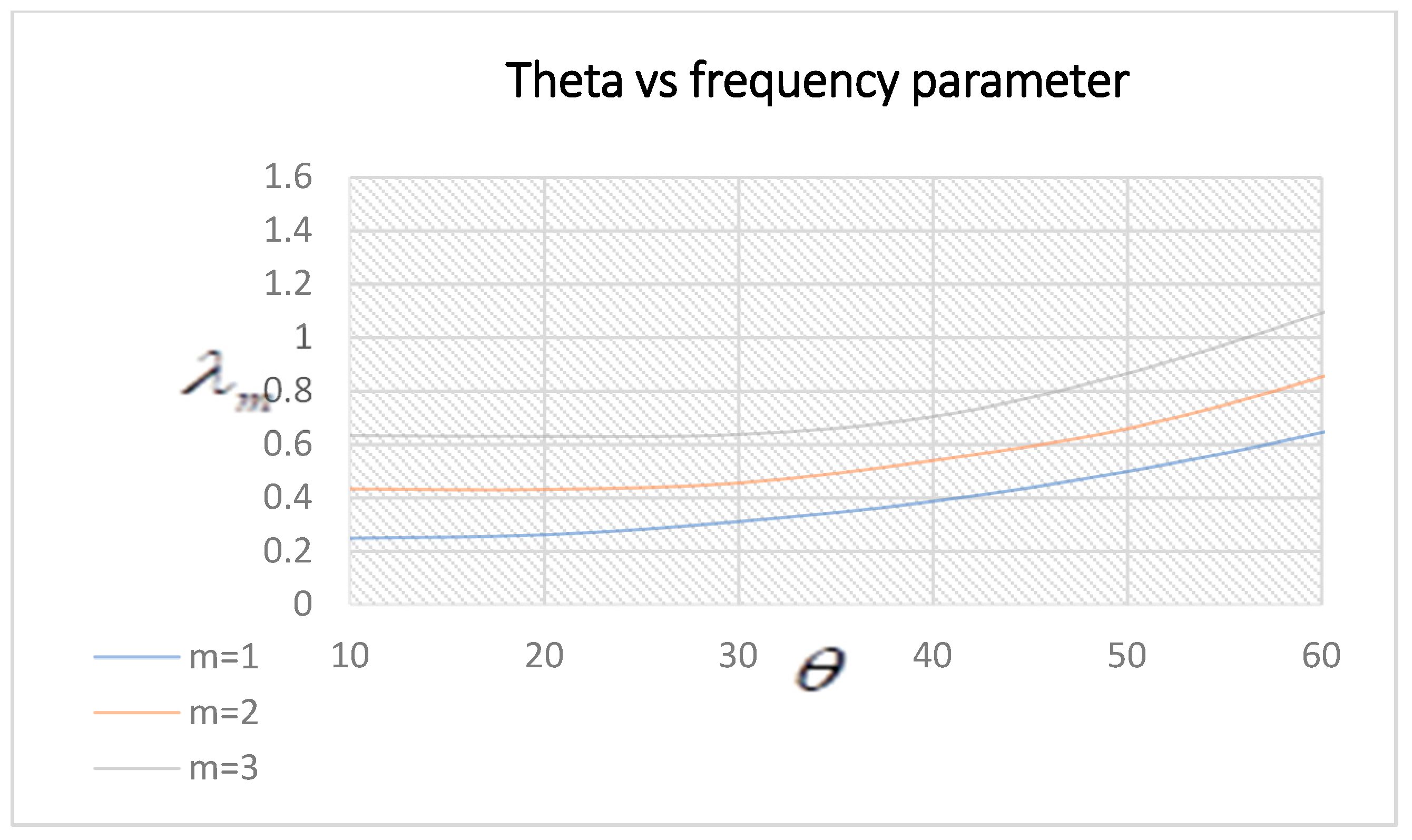
Table 3 shows that the value of the frequency parameter increases with the increase in ply angle. It also depicts that as the number of layers of composite plates decreases the frequency, the parameter value also decreases. It is known that the stiffness decrease or increase according to the frequency parameter value decreases or increases. In this study, as the number of layers of plates decreases, the frequency parameter value also decreases, which shows that its stiffness decreases and flexibility increases.
3.4. Frequency Parameter Variation under the Effect of the Aspect Ratio, Side-to-Thickness Ratio, and Ply Angle of Symmetric Plates
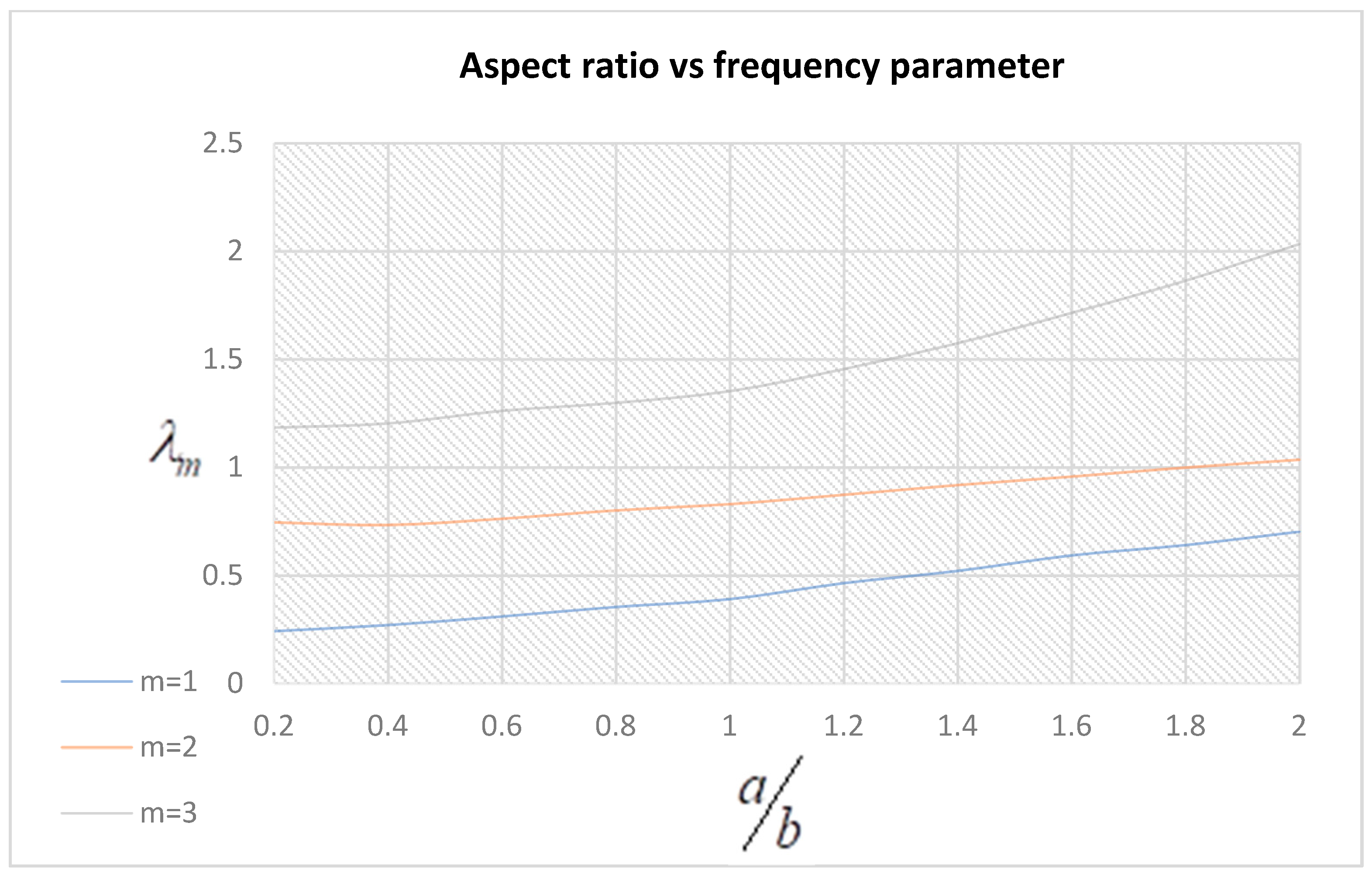
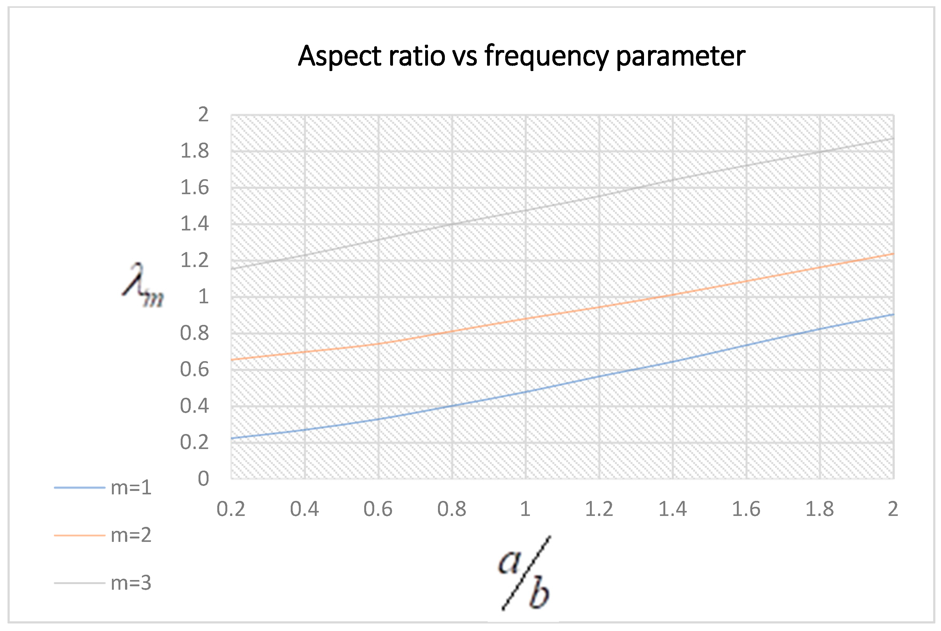
Figure 2, Figure 3 and Figure 4 show the effect of the aspect ratio on the frequency parameter of symmetric angle ply plates of 6-layered plates under simply supported boundary conditions. Different ply angle orientations were used. It shows that as the aspect ratio increases, the frequency increases gradually. This shows that the rigidity of the structure increases with the increase in frequency values and its flexibility decreases.
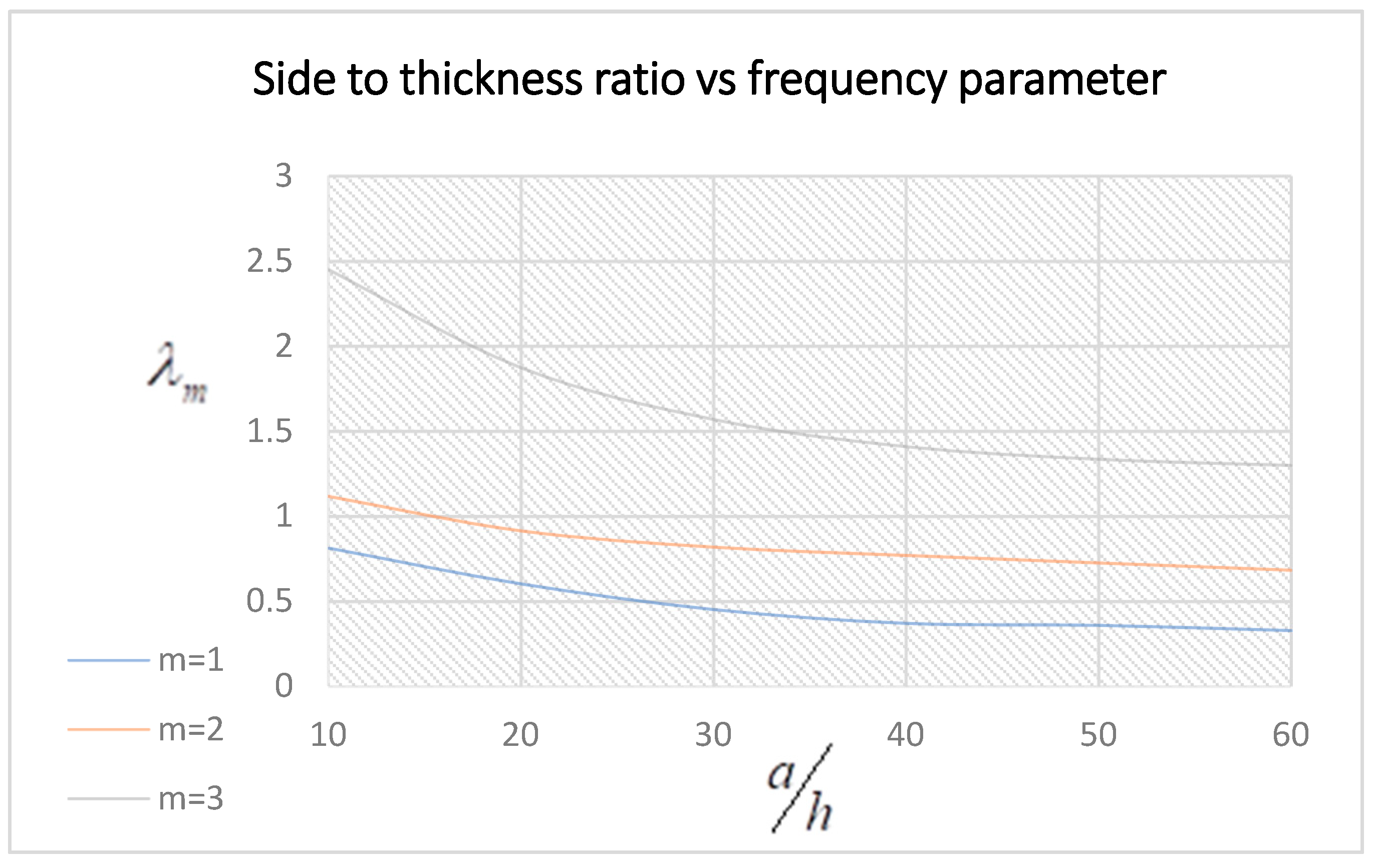
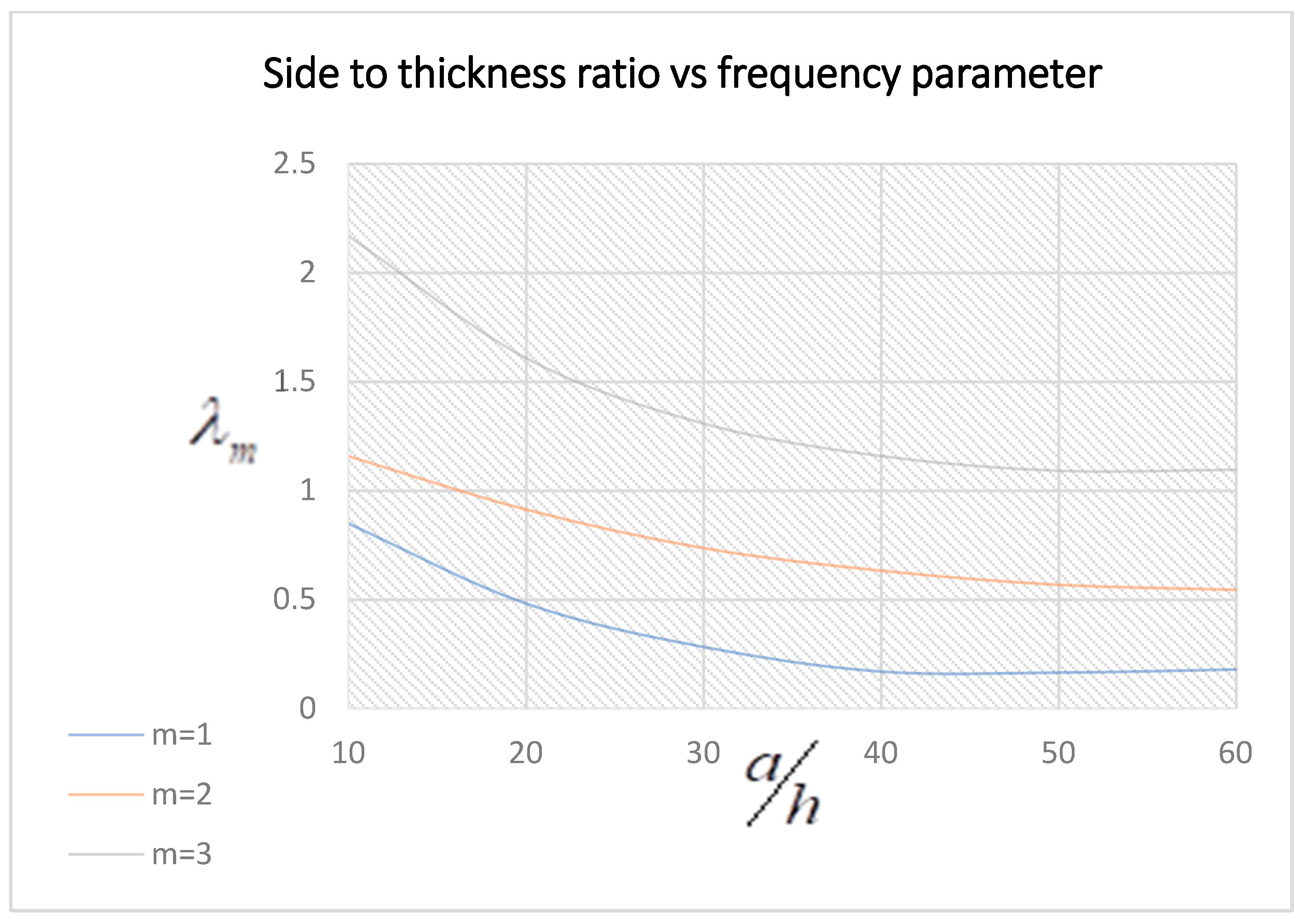
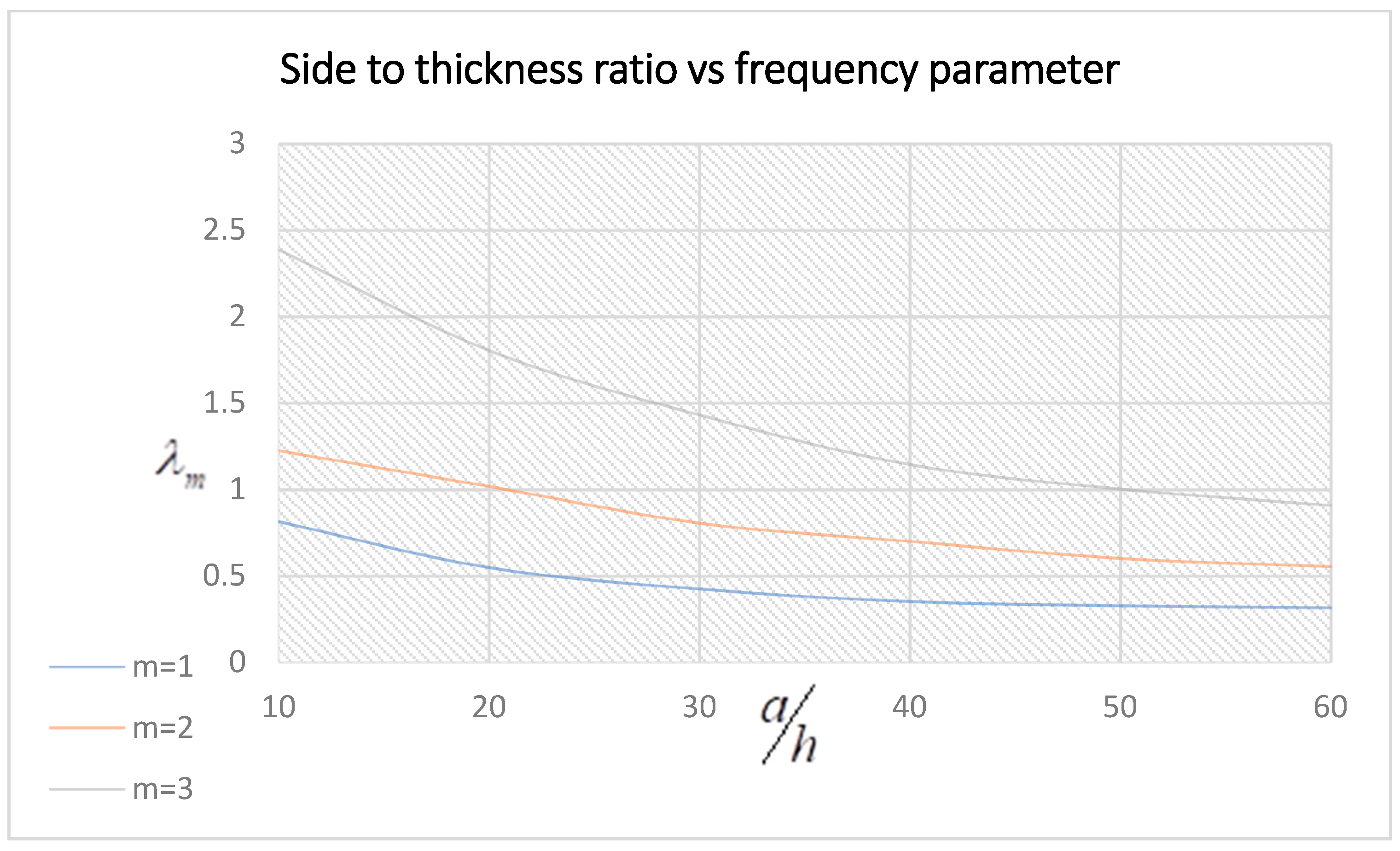
Figure 5, Figure 6 and Figure 7 demonstrate the variation of the side-to-thickness ratio and frequency parameter of plates of different symmetric ply orientations. The curvature of the graph curve elucidates that as the side-to-thickness ratio value increases, the frequency parameter value decreases.
4. Conclusions
The research provides a numerical analysis solution for symmetric angle ply plates using HSDT under simply supported support conditions. The results obtained from the research can be used to study the frequency response of the plate and the parametric effects of various plate configurations. The research highlights the importance of considering the aspect ratio and the side-to-thickness ratio when designing symmetric angle ply plates. The effect of the aspect ratio on the frequency parameter is that with the increase in the aspect ratio, the frequency increases gradually. Moreover, as the side-to-thickness ratio increases, the frequency parameter value decreases. In addition to this, as the ply angle increases, the frequency value also increases. It is evident from these results that as the number of layers of plates decreases, the frequency parameter value also decreases, which shows that as the stiffness of a structure decreases, the flexibility increases. However, with the increase in the aspect ratio and the side-to-thickness ratio, the frequency increases, which shows that as the rigidity of a structure increases, the flexibility decreases.
The obtained results are validated by existing literature.
Funding
This research and APC was supported and funded by [Deanship of Scientific Research, Vice Presidency for Graduate Studies and Scientific Research, King Faisal University, Saudi Arabia] Project No. GRANT3,089.
Data Availability Statement
The data supporting the results of this study are included in the manuscript.
Acknowledgments
This work was completed by Saira Javed and supported by the Deanship of Scientific Research, Vice Presidency for Graduate Studies and Scientific Research, King Faisal University, Saudi Arabia [Project No. GRANT3,089].
Conflicts of Interest
The author declares that they have no conflicts of interest regarding the publication of this paper.
Nomenclature
| Elastic coefficients representing the extensional rigidity | |
| Elastic coefficients representing the bending–stretching coupling rigidity | |
| Elastic coefficients representing the bending rigidity | |
| Shear modulus in the respective directions of the k-th layer | |
| Side-to-thickness ratio | |
| The Heaviside step function | |
| Normal inertia coefficient | |
| Rotary inertia coefficients | |
| Length parameter | |
| Moment resultants in the respective directions of the plate | |
| Stress results in the respective direction of the plate | |
| Number of intervals of spline interpolation | |
| Elements of the stiffness matrix for the material of the k-th layer | |
| Elements of the transformed stiffness matrix for the material of the k-th layer | |
| Transverse shear resultants in the respective directions of the plate | |
| Displacement functions in the , , and directions of the plate | |
| Nondimensionalized distance co-ordinate of the plate | |
| The equally spaced knots of spline interpolation | |
| , | Length and width of the plates |
| , | Spline coefficients |
| The total thickness of the plate | |
| The thickness of the k-th layer of the plate | |
| Summation or general indices | |
| , , and displacements of the plate | |
| The in-plane displacements of the reference surface | |
| Length coordinate of the plate | |
| Width coordinate of the plate | |
| Normal coordinate of any point on the plate | |
| Distance of the top of the k-th layer from the reference surface | |
| Product of of the plate | |
| The relative layer thickness of the -th layer | |
| Normal strain in the respective directions | |
| Shear strain in the respective directions of the plate | |
| The changes in the curvature of the reference surface during deformation in the respective directions of the plate Non-dimensional frequency parameter | |
| Shear rotations of any point on the middle surface of the plate | |
| Shear rotational functions of the plate | |
| Non-dimensionalized shear rotations of the plate | |
| The mass density of the material of the plate or shell | |
| Normal stress in the respective directions of the plate | |
| Shear stress at a point on the reference surface of the plate | |
| Ply orientation angle |
Appendix A
Appendix A.1. Components of the Stiffness Matrix for the of k-th Layer of Plate Material
Appendix A.2. Components of the Transformed Stiffness Matrix for the k-th Layer Material
References
- Vinson, J.R. Sandwich Structures. Appl. Mech. Rev. 2001, 54, 201–214. [Google Scholar] [CrossRef]
- Noor, A.K.; Burton, W.S.; Bert, C.W. Computational models for sandwich panels and shells. Appl. Mech. Rev. 1996, 49, 155–199. [Google Scholar] [CrossRef]
- Yang, P.C.; Nooris, C.H.; Stavsky, Y. Elastic wave propogation in heterogeneous plates. Int. J. Solids Struct. 1966, 2, 665–684. [Google Scholar] [CrossRef]
- Reddy, J.N. Theory and Analysis of Elastic Plates and Shells; CRC Press: Boca Raton, FL, USA, 2006. [Google Scholar]
- Ghiamy, A.; Amoushahi, H. Dynamic stability of different kinds of sandwich plates using third order shear deformation theory. Thin-Walled Struct. 2022, 172, 108822. [Google Scholar] [CrossRef]
- Parida, S.P.; Jena, P.C. Free and forced vibration analysis of flyash/graphene filled laminated composite plates using higher order shear deformation theory. Proc. Inst. Mech. Eng. Part C J. Mech. Eng. Sci. 2022, 236, 4648–4659. [Google Scholar] [CrossRef]
- Zhao, Y.; Qin, B.; Wang, Q.; Liang, X. A unified Jacobi–Ritz approach for the FGP annular plate with arbitrary boundary conditions based on a higher-order shear deformation theory. J. Vib. Control 2022. [Google Scholar] [CrossRef]
- Tian, Y.; Li, Q.; Wu, D.; Chen, X.; Gao, W. Nonlinear dynamic stability analysis of clamped and simply supported organic solar cells via the third-order shear deformation plate theory. Eng. Struct. 2022, 252, 113616. [Google Scholar] [CrossRef]
- Belkhodja, Y.; Ouinas, D.; Fekirini, H.; Olay, J.A.; Achour, B.; Touahmia, M.; Boukendakdji, M. A new hybrid HSDT for bending, free vibration, and buckling analysis of FGM plates (2D & quasi-3D). Smart Struct. Syst. 2022, 29, 395–420. [Google Scholar]
- Eskandari Shahraki, M.; Shariati, M.; Asiaban, N.; Davar, A.; Heydari Beni, M.; Eskandari Jam, J. Assessment of Third-order Shear Deformation Graphene Nanoplate Response under Static Loading Using Modified Couple Stress Theory. J. Mod. Process. Manuf. Prod. 2022, 11, 41–57. [Google Scholar]
- Shi, P.; Dong, C. A refined hyperbolic shear deformation theory for nonlinear bending and vibration isogeometric analysis of laminated composite plates. Thin-Walled Struct. 2022, 174, 109031. [Google Scholar] [CrossRef]
- Javani, M.; Kiani, Y.; Eslami, M.R. On the free vibrations of FG-GPLRC folded plates using GDQE procedure. Compos. Struct. 2022, 286, 115273. [Google Scholar] [CrossRef]
- Sayyad, A.S.; Avhad, P.V. A new higher order shear and normal deformation theory for the free vibration analysis of sandwich curved beams. Compos. Struct. 2022, 280, 114948. [Google Scholar] [CrossRef]
- Ellali, M.; Bouazza, M.; Amara, K. Thermal buckling of a sandwich beam attached with piezoelectric layers via the shear deformation theory. Arch. Appl. Mech. 2022, 92, 657–665. [Google Scholar] [CrossRef]
- Nguyen, N.D.; Nguyen, T.N.; Nguyen, T.K.; Vo, T.P. A new two-variable shear deformation theory for bending, free vibration and buckling analysis of functionally graded porous beams. Compos. Struct. 2022, 282, 115095. [Google Scholar] [CrossRef]
- Peng, L.X.; Chen, S.Y.; Wei, D.Y.; Chen, W.; Zhang, Y.S. Static and free vibration analysis of stiffened FGM plate on elastic foundation based on physical neutral surface and MK method. Compos. Struct. 2022, 290, 115482. [Google Scholar] [CrossRef]
- Pham, Q.H.; Tran, T.T.; Tran, V.K.; Nguyen, P.C.; Nguyen-Thoi, T. Free vibration of functionally graded porous non-uniform thickness annular-nanoplates resting on elastic foundation using ES-MITC3 element. Alex. Eng. J. 2022, 61, 1788–1802. [Google Scholar] [CrossRef]
- Hung, P.T.; Phung-Van, P.; Thai, C.H. A refined isogeometric plate analysis of porous metal foam microplates using modified strain gradient theory. Compos. Struct. 2022, 289, 115467. [Google Scholar] [CrossRef]
- Sharma, N.; Swain, P.K.; Maiti, D.K.; Singh, B.N. Static and free vibration analyses and dynamic control of smart variable stiffness laminated composite plate with delamination. Compos. Struct. 2022, 280, 114793. [Google Scholar] [CrossRef]
- Cho, J.R. Nonlinear free vibration of functionally graded CNT-reinforced composite plates. Compos. Struct. 2022, 281, 115101. [Google Scholar] [CrossRef]
- Zang, Q.; Liu, J.; Ye, W.; Yang, F.; Hao, C.; Lin, G. Static and free vibration analyses of functionally graded plates based on an isogeometric scaled boundary finite element method. Compos. Struct. 2022, 288, 115398. [Google Scholar] [CrossRef]
- Ghosh, S.; Haldar, S. Free Vibration analysis of isotropic and laminated composite plate on elastic point supports using finite element method. In Recent Advances in Computational and Experimental Mechanics; Springer: Singapore, 2022; Volume II, pp. 371–384. [Google Scholar]
- Milazzo, A. Free vibrations analysis of cracked variable stiffness composite plates by the extended Ritz method. Mech. Adv. Mater. Struct. 2022. [Google Scholar] [CrossRef]
- Saiah, B.; Bachene, M.; Guemana, M.; Chiker, Y.; Attaf, B. On the free vibration behavior of nanocomposite laminated plates contained piece-wise functionally graded graphene-reinforced composite plies. Eng. Struct. 2022, 253, 113784. [Google Scholar] [CrossRef]
- Singh, A.; Karathanasopoulos, N. Three-dimensional analytical elasticity solution for the mechanical analysis of arbitrarily-supported, cross and angle-ply composite plates under patch loads. Compos. Struct. 2023, 310, 116752. [Google Scholar] [CrossRef]
- Belardi, V.G.; Fanelli, P.; Vivio, F. Application of the Ritz method for the bending and stress analysis of thin rectilinear orthotropic composite sector plates. Thin-Walled Struct. 2023, 183, 110374. [Google Scholar] [CrossRef]
- Zhong, R.; Hu, S.; Liu, X.; Qin, B.; Wang, Q.; Shuai, C. Vibro-acoustic analysis of a circumferentially coupled composite laminated annular plate backed by double cylindrical acoustic cavities. Ocean. Eng. 2022, 257, 111584. [Google Scholar] [CrossRef]
- Wang, H.; Zhao, X.; Gao, H.; Yuan, T.; Liu, X.; Zhang, W. Effects of alkali-treated plant wastewater on the properties and microstructures of alkali-activated composites. Ceram. Int. 2023, 49, 8583–8597. [Google Scholar] [CrossRef]
- Zhang, Y.; Liu, G.; Ye, J.; Lin, Y. Crushing and parametric studies of polygonal substructures based hierarchical cellular honeycombs with non-uniform wall thickness. Compos. Struct. 2022, 299, 116087. [Google Scholar] [CrossRef]
- Zhang, H.; Ouyang, Z.; Li, L.; Ma, W.; Liu, Y.; Chen, F.; Xiao, X. Numerical study on welding residual stress distribution of corrugated steel webs. Metals 2022, 12, 1831. [Google Scholar] [CrossRef]
- Peng, J.; Xu, C.; Dai, B.; Sun, L.; Feng, J.; Huang, Q. Numerical Investigation of Brittleness Effect on Strength and Microcracking Behavior of Crystalline Rock. Int. J. Geomech. 2022, 22, 04022178. [Google Scholar] [CrossRef]
- Reddy, J.N. Mechanis of Laminated Composite Plates and Shells; CRC Press: Boca Raton, FL, USA, 2003. [Google Scholar]
- Schoenberg, I.J.; Whitney, A. On Pólya frequence functions. III. The positivity of translation determinants with an application to the interpolation problem by spline curves. Trans. Am. Math. Soc. 1953, 74, 246–259. [Google Scholar] [CrossRef] [Green Version]
- Shi, J.W.; Nakatani, A.; Kitagawa, H. Vibration analysis of fully clamped arbitrarily laminated plate. Compos. Struct. 2004, 63, 115–122. [Google Scholar] [CrossRef]
- Xiang, S.; Jiang, S.X.; Bi, Z.Y.; Jin, Y.X.; Yang, M.S. A nth-order meshless generalization of Reddy’s third-order shear deformation theory for the free vibration on laminated composite plates. Compos. Struct. 2011, 93, 299–307. [Google Scholar] [CrossRef]
Figure 1.
Composite plate geometry.

Figure 2.
Variation of the aspect ratio vs. frequency parameter of 6-layered plates .

Figure 3.
Variation of the aspect ratio vs. frequency parameter of 6-layered plates .

Figure 4.
Variation of the aspect ratio vs. frequency parameter of 6-layered plates .

Figure 5.
Variation of the side-to-thickness ratio vs. frequency parameter of 5-layered plates .

Figure 6.
Variation of side-to-thickness ratio vs. frequency parameter of 6-layered plates .

Figure 7.
Variation of side-to-thickness ratio vs. frequency parameter of 6-layered plates .

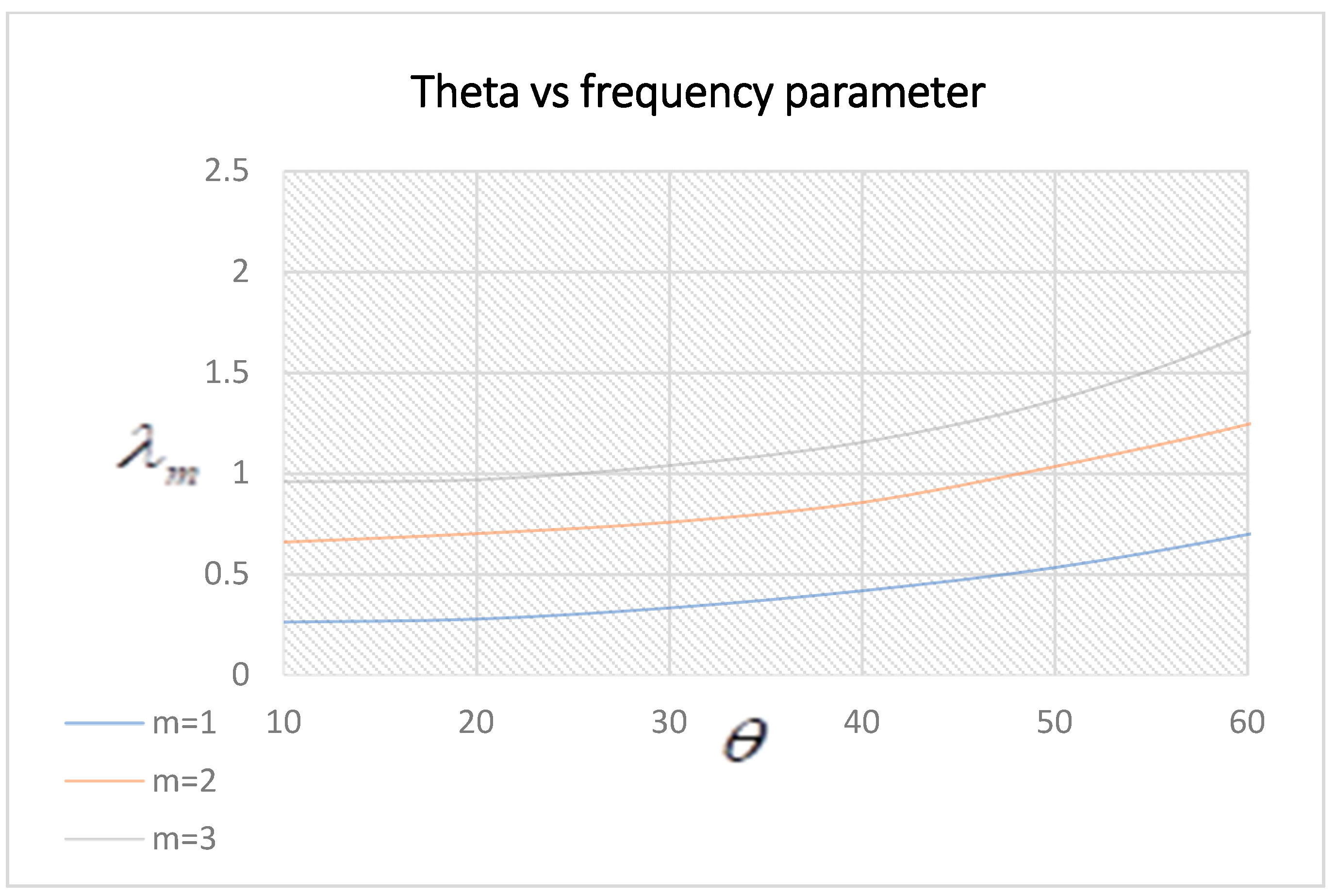
Figure 8.
Variation of the theta vs. frequency parameter of 6-layered plates.

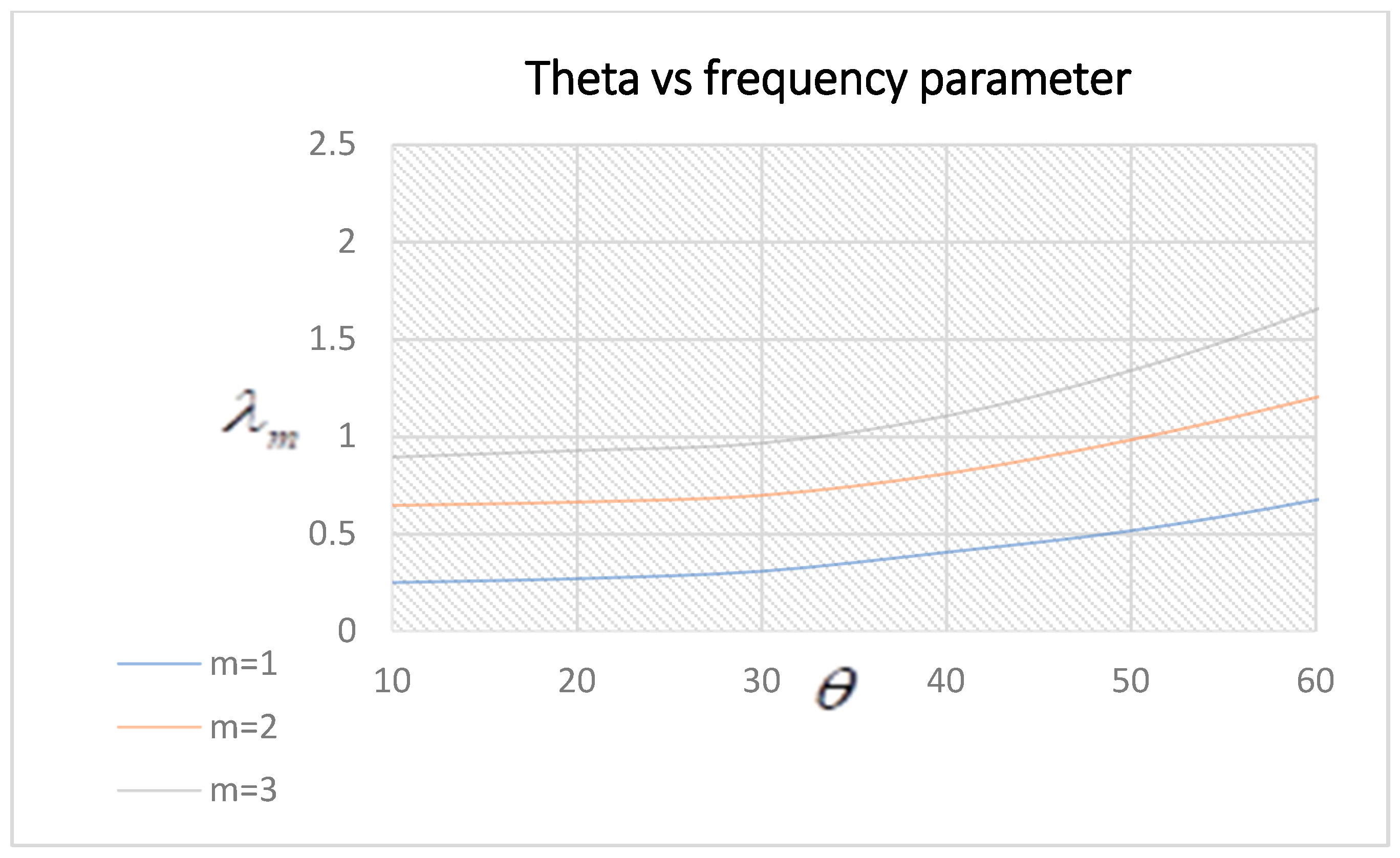
Figure 9.
Variation of the theta vs. frequency parameter of 5-layered plates.

Figure 10.
Variation of the theta vs. frequency parameter of 3-layered plates.


Table 1.
Convergence for the frequency parameters of four layered anti-symmetric plates under C-C boundary conditions.
Table 1.
Convergence for the frequency parameters of four layered anti-symmetric plates under C-C boundary conditions.
| % Change | % Change | % Change | ||||
|---|---|---|---|---|---|---|
| 4 | 0.547064 | - | 1.260471 | - | 2.0610 | - |
| 6 | 0.511985 | −6.41222 | 1.12029 | −11.12131 | 1.894131 | −8.09650 |
| 8 | 0.499459 | −2.46555 | 1.069711 | −4.51481 | 1.761941 | −6.97892 |
| 10 | 0.493624 | −1.16826 | 1.046288 | −2.18965 | 1.700053 | −3.51248 |
| 12 | 0.490446 | −0.64380 | 1.033585 | −1.21410 | 1.666535 | −1.97158 |
Table 2.
Comparison of non-dimensional frequencies of square clamped supported plate with . Results are compared with Shi et al. [34] and Xiang et al. [35].
| Method | Mode 1 | 2 | 3 | |
|---|---|---|---|---|
| 10 | Shi et al. [34] Xiang et al. [35] Present | 17.433 17.225 17.333 | 22.506 22.261 22.576 | 30.905 30.631 30.981 |
| 20 | Shi et al. [34] Xiang et al. [35] Present | 23.979 23.745 23.854 | 30.407 30.041 30.342 | 41.937 41.295 41.821 |
| 100 | Shi et al. [34] Xiang et al. [35] Present | 28.946 28.572 28.734 | 36.772 36.184 36.634 | 50.721 49.791 50.612 |
Table 3.
The fundamental frequency of different layered plates by varying ply angles.
| 6-Layered | 5-Layered | 3-Layered | |
|---|---|---|---|
| 0.262205 | 0.249637 | 0.246888 | |
| 0.276866 | 0.269521 | 0.259949 | |
| 0.332592 | 0.307604 | 0.309678 | |
| 0.417498 | 0.404969 | 0.385188 | |
| 0.53254 | 0.515285 | 0.497382 | |
| 0.696845 | 0.673437 | 0.643287 | |
| 0.899267 | 0.869292 | 0.83807 |
Disclaimer/Publisher’s Note: The statements, opinions and data contained in all publications are solely those of the individual author(s) and contributor(s) and not of MDPI and/or the editor(s). MDPI and/or the editor(s) disclaim responsibility for any injury to people or property resulting from any ideas, methods, instructions or products referred to in the content. |
© 2023 by the author. Licensee MDPI, Basel, Switzerland. This article is an open access article distributed under the terms and conditions of the Creative Commons Attribution (CC BY) license (https://creativecommons.org/licenses/by/4.0/).
Share and Cite
MDPI and ACS Style
Javed, S. A Numerical Solution of Symmetric Angle Ply Plates Using Higher-Order Shear Deformation Theory. Symmetry 2023, 15, 767. https://doi.org/10.3390/sym15030767
AMA Style
Javed S. A Numerical Solution of Symmetric Angle Ply Plates Using Higher-Order Shear Deformation Theory. Symmetry. 2023; 15(3):767. https://doi.org/10.3390/sym15030767
Chicago/Turabian StyleJaved, Saira. 2023. "A Numerical Solution of Symmetric Angle Ply Plates Using Higher-Order Shear Deformation Theory" Symmetry 15, no. 3: 767. https://doi.org/10.3390/sym15030767
Note that from the first issue of 2016, this journal uses article numbers instead of page numbers. See further details here.