A Comprehensive Analysis of Smart Grid Stability Prediction along with Explainable Artificial Intelligence

Abstract

As the backbone of modern society and industry, the need for a more efficient and sustainable electrical grid is crucial for proper energy management. Governments have recognized this need and have included energy management as a key component of their plans. Decentralized Smart Grid Control (DSGC) is a new approach that aims to improve demand response without the need for major infrastructure upgrades. This is achieved by linking the price of electricity to the frequency of the grid. While DSGC solutions offer benefits, they also involve several simplifying assumptions. In this proposed study, an enhanced analysis will be conducted to investigate how data analytics can be used to remove these simplifications and provide a more detailed understanding of the system. The proposed data-mining strategy will use detailed feature engineering and explainable artificial intelligence-based models using a public dataset. The dataset will be analyzed using both classification and regression techniques. The results of the study will differ from previous literature in the ways in which the problem is handled and the performance of the proposed models. The findings of the study are expected to provide valuable insights for energy management-based organizations, as it will maintain a high level of symmetry between smart grid stability and demand-side management. The proposed model will have the potential to enhance the overall performance and efficiency of the energy management system.

1. Introduction

1.1. Motivation

In terms of energy sustainability and resiliency, the smart grid (SG) has an important role. The path to predictable and manageable energy policies comes across the digitalization of the electrical grid itself. While SG infrastructures exist, it still has the potential to be developed and enhanced with effective interfaces. There are still compelling topics in the application of SG in the field. Renewable energy integration takes the lead for those important issues [1]. Adapting renewable energy resources to the conventional grid may cause problems. Contrary to the traditional system, those bi-directional ways of production define new consumer models. While there were just a few power plants as a center of production in the conventional grid, the SG structure with the integration of alternative generation centers comes with a “prosumers” definition. As we can infer from the name, those prosumers produce the energy like the power plants but also consume it too. This symmetric flow builds the aforementioned bi-directional way of production [2]. Thinking of those all together may lead to a complicated way of planning the generation, distribution, and consumption of electrical energy. In such a plan, there is an important decision for every player in the field: is it a feasible step to buy the energy or not buy it at a particular price? At the present, the end-users of industrial fields and also residential areas have their electricity generated locally by themselves, these distributed energy resources are very common, too. Over and above that, the SG infrastructure itself has very complicated types of equipment for monitoring and self-healing applications [3]. Those collective considerations and the necessity for the proper decision-making strategy have devotedly underlined the smart grid stability analysis [4].

Electrical grid topology, with its symmetrical structure, should provide a balanced power flow between the supply center and the consumer (demand) side to achieve stability. The stability definition here should not be mixed up with frequency or voltage stability in particular. The stability definition is more like the balance term, which is between the generation center and demand side. In demand-side management and prosumers’ behavior price allocation is an important issue. Price policies and changes in tariffs are strongly dependent on electricity consumption and production link. In the literature, there are so many approaches presented to describe the price determination and make the consumers informed of it [5,6]. Traditional methods, such as local electricity auctions, may lead to cyber security gaps and privacy issues [7]. Overcoming the mentioned issues, the decentralized smart grid control (DSGC) has been recently announced to the academic audience by the studies [8,9]. Connecting the frequency of SG directly to the price of electricity provides fewer communication channels for sharing the price info between all the players in the game, namely producers and consumers. Thanks to this unique feature, DSGC tends to produce the pricing policy in a real-time manner, contrary to the auctions in which price trading is handled with 15-min time intervals [5].

DSGC methodology takes advantage of the frequency info of the grid itself. The frequency keeps a secret knowledge in its increase and decrease. When the generation of electricity increases for the whole balanced system of participants of the SG, the electrical frequency of the grid also increases, and vice versa, in an underproduction situation, the electrical frequency of the grid decreases along with it. This leads to the conclusion that all the necessary information for determining electricity prices can be obtained from frequency measurements [8,10]. On that account, the frequency information of each participant of the grid would be sufficient to obtain the necessary details to sign a balanced power flow of the grid. For a network operation aiming the electricity price regulation, and informing the consumers, those steps would be a very shortcut in the field [10].

For all those important points of the DSGC methodology, aiming to provide comprehensive data analytics with the help of artificial intelligence would be the very beginning of this study. Within the framework of this comprehensive analysis, it is aimed to enlighten the SG stability prediction with feature engineering and enhanced deep learning and machine learning-based models. Moreover, the analysis in this study collects the results of similar studies using the same datasets and interprets the big picture as a meta-analysis.

1.2. Problem

DSGC approach analyses the SG stability phenomenon using mathematical models with differential equations. The studies [8,9] that presented the fundamental theory of the DSGC considered the test-bed electrical grid as a four-node star topology involving an energy source (generation node) and three nodes denoting the consumption. In the theory of the DSGC, input features of the system are considered as listed: The summed power balance of which the produced or consumed power values of each node; the time value that related to responses of consumers/prosumers whether production or consumption is feasible for current price values, i.e., reaction time, and the price elasticity of the produced energy [5].

Thinking over the system parameters, it can be inferred that a complete and concise mathematical model can be pictured for the prediction of SG stability. We can conduct the SG stability analysis as a classification or regression problem. Nevertheless, some major assumptions are addressed in the solution for this model. As brightly explained in [5], mathematical models that involve differential equations can be solved in various ways. In the process, there can be simulations operated with a collection of constant values for a single variable set and assuming fixed distributions for the rest of the variable set. We can name two negative situations on this matter, equality, and fixed inputs. In this study, the main problem on the desk is to provide a solution to those issues in the way of SG stability prediction. This prospective study was designed to investigate the solution for the problems that have been faced in the way of SG stability prediction. A holistic approach is used, integrating feature engineering and modern artificial intelligence techniques to establish a robust analysis of SG stability prediction in classification and regression manners.

As for the problem definition, the proposed study deals with the drawbacks of the existing SG stability analysis in DSGC.

Decentralized smart grid control has several advantages over traditional centralized grid control systems [8]:

• Increased reliability: Decentralized systems can help to improve grid reliability by distributing generation and storage resources across the grid, reducing the impact of individual failures or outages.
• Improved grid efficiency: Decentralized systems can help to optimize the use of generation and storage resources, leading to more efficient use of energy and lower costs for customers.
• Greater integration of renewable energy: Decentralized systems can facilitate the integration of renewable energy sources, such as solar and wind power, into the grid by allowing for more precise and dynamic control of these resources.
• Increased customer choice: Decentralized systems can give customers more control over their energy consumption and costs, by allowing them to choose how and when they use energy, and to participate in demand response programs.
• Reduced transmission and distribution costs: Decentralized systems can reduce the need for expensive transmission and distribution infrastructure by allowing energy to be generated and consumed closer to where it is needed.
• Increased security of the grid: Decentralized systems can increase the overall security of the grid by making it more resilient to cyber-attacks.

Overall, decentralized smart grid control can help to improve the efficiency, reliability, and security of the grid while also providing more choice and control to customers and supporting the integration of renewable energy sources. Despite the abovementioned advantages of DSGC, we still have some problems in the process.

One major challenge is maintaining power quality and stability on the grid, as the distributed nature of distributed energy resources can make it difficult to predict and control power flows. In addition, coordinating the operation of multiple distributed energy resources in real-time can be complex and computationally intensive. The proposed study gives a solution for stability prediction to this problem.

1.3. Related Works

Firstly, in 2015 and 2016, Schäfer et al. defined the DSGC in [8,9]  by publishing the studies one after another. They draw the big picture of DSGC, describing the pros and cons of its methodology. Taking those studies to the basis, Arzamasov et al. discussed SG stability in a conference by describing their concise models [5]. Along with the study [5], Arzamasov et al. shared a comprehensive dataset to provide the researchers with conduct the SG stability analysis overcoming the DSGC issues in a University of California Irvine (UCI) machine learning data repository. In their study, they proposed a basic decision tree model to predict SG stability with some analysis of DSGC methodology. In 2019, Moldovan et al. discussed the instability factors using the dataset of Arzamasov’s team (raw dataset) in the study [11]. In their study, they designed their methodology on classical machine learning methodology by using a bunch of basic models. A year later in 2020, Alazab et al. proposed a long-short-term memory (LSTM) based prediction model for SG stability using the basic dataset [12]. They emphasized the subject of taking the cyber-physical system definition into account. A bundle deep learning (DL) based model has been designed for the stability prediction process. After that period, in the same year, Paulo Breviglieri generated an augmented version of the dataset of Arzamasov’s team and shared it in the Kaggle data repository. Following this, Breviglieri et al. published an article in 2021 covering the SG stability prediction by analyzing the augmented dataset [10]. Li proposed a set of machine learning models based on conventional algorithms using the raw dataset to analyze the SG stability index [13]. Bashir et al. proposed a list of machine-learning models for the SG stability prediction on the raw dataset. The study also includes artificial neural networks (ANN) based classifiers [14]. The last study in the literature using the raw dataset was proposed by Massaoudi et al. [15]. The authors use LSTM-based models to predict the SG stability index considering it a regression problem. To this point, study [15] is the only approach for handling the stability prediction as a regression model. The author of the proposed (current ) study also conferred an abstract presentation on smart grid stability prediction with the augmented dataset by using a lightweight convolutional neural network (CNN) deep learning classifier [16]. The former study just included a basic classifier without any data analysis or feature engineering.

Apart from the existing studies in the literature whose datasets are raw and augmented datasets, the proposed study considers both raw and augmented datasets together in the way of SG stability prediction. Thus, by the collection of both data packages, it is enlightened that the augmentation process over the raw dataset whether effective or not. Using the advantage of feature engineering and data analytics, this study takes the SG stability prediction a few steps forward with the explainable artificial intelligence (XAI) [17,18]. The comprehensive analysis also handles the SG prediction as both classification and regression problems with the state-of-the-art machine learning model gradient boosting machine [19] and deep models.

1.4. Contribution

The remarkable contributions of the proposed study can be listed as:

• Analyzed existing SG stability datasets using data analytics, detailed feature engineering, and XAI.
• Interpretability of the proposed research sets our study apart from existing ones in the literature.
• To the best of the author’s knowledge, this is the first study that comprehensively handles both raw and augmented SG stability datasets as both classification and regression problems with a symmetrical approach.
• Utilized state-of-the-art gradient boosting machine and deep learning models to design AI-based SG stability prediction models with higher performance values compared to existing studies in the literature.

1.5. Outline of the Article

Following the introduction section, Section 2 contains the materials and methods. In its sub-sections, we can follow the dataset definition, feature engineering, and prediction models. Section 3 deals with the results and discussion. Section 4 provides a brief conclusion of the proposed study.

2. Materials and Methods

In this section, the handled SG stability datasets are described with their prominent specifications. For the next step, the feature engineering and data analytic details are given. Lastly, the machine learning and deep learning-based models are explained in a brief manner.

2.1. Dataset Definition

In this study, the two benchmark datasets used in SG stability prediction have been considered. The first one we can name is the raw dataset which was prepared by Arzamasov et al. and their research team [5]. The latter one we can name is the augmented dataset which was first used in the study of Breviglieri et al. [10]. Both datasets include the same feature and target (response) columns. The difference is the data volume of datasets. While the raw dataset contains 10K samples, the augmented dataset contains 60K samples. The datasets are built with the realistic simulation results of smart grid stability operations where a four-node topology is considered. The “four” total nodes are the sum of a generation center node and three consumer nodes. Both raw and augmented datasets are involved twelve attributes (features) and two dependent labels. While one dependent variable suits the classification problem, the other suits the regression problem. Using these two dependent labels altogether is not logical when handling the problem from a classification and regression perspective. For this reason, the proposed models consider the two dependent labels of the datasets separately for the classification and regression approaches.

Table 1. Feature Details for raw and augmented datasets.

Symbol	Description	Name
P	Nominal power values of GN and CNs	p1 to p4
$\tau$	Reaction time values of GN and CNs	tau1 to tau4
$\gamma$	Gamma coefficient, price elasticity for GN and CNs	g1 to g4

gives the feature details of both datasets for generation nodes (GN) and consumer nodes (CNs).

As dependent variables, we can list “stab” and “stabf”. The former is the root of the differential equation (when this value is positive, then the grid is linearly unstable; if it is negative, then the grid is stable), and the latter is a categorical value defining the grid situation as stable and unstable which is a binary label. This depicts that those two dependent variables are stuck to each other with a direct relationship. Because of this, the numerical variables “stab” should be picked for the regression approach by dropping the “stabf” response. The “stabf” response should be picked for the classification approach by dropping the “stab” response. In this study, these two situations are handled separately under the name of classification approach and regression approach. In both datasets, there are no missing values. As our machine learning and deep models accept categorical responses, so there is no need for a detailed data pre-processing stage. The datasets were seamlessly generated. The next section gives the feature engineering results along with feature visualizations and statistical relationships.

2.2. Data Analytics and Feature Engineering

2.2.1. Analytics of Raw (10K) Dataset

To put both datasets on the table on the way to provide comprehensive data analytics, we will see a set of statistical demonstrations in this sub-section. Starting with a basic statistical measure of the raw dataset,

Table 2. Statistical details of raw dataset.

Features	Count	Mean	Std	Min	25%	50%	75%	Max
tau1	10,000	5.25	2.742548	0.500793	2.874892	5.250004	7.62469	9.999469
tau2	10,000	5.250001	2.742549	0.500141	2.87514	5.249981	7.624893	9.999837
tau3	10,000	5.250004	2.742549	0.500788	2.875522	5.249979	7.624948	9.99945
tau4	10,000	5.249997	2.742556	0.500473	2.87495	5.249734	7.624838	9.999443
p1	10,000	3.75	0.75216	1.58259	3.2183	3.751025	4.28242	5.864418
p2	10,000	−1.25	0.433035	−1.999891	−1.624901	−1.249966	−0.874977	−0.500108
p3	10,000	−1.25	0.433035	−1.999945	−1.625025	−1.249974	−0.875043	−0.500072
p4	10,000	−1.25	0.433035	−1.999926	−1.62496	−1.250007	−0.875065	−0.500025
g1	10,000	0.525	0.274256	0.050009	0.287521	0.525009	0.762435	0.999937
g2	10,000	0.525	0.274255	0.050053	0.287552	0.525003	0.76249	0.999944
g3	10,000	0.525	0.274255	0.050054	0.287514	0.525015	0.76244	0.999982
g4	10,000	0.525	0.274255	0.050028	0.287494	0.525002	0.762433	0.99993
stab	10,000	0.015731	0.036919	−0.08076	−0.015557	0.017142	0.044878	0.109403

shows important values. We can see the basic statistics like the mean, standard deviation (std), minimum (min), and maximum (max) values with the distribution portions of quartile percentages.

As we can see in the mean and std columns, the groups of features have nearly the same mean and std values except for the p1 feature. This is because the p1 feature addresses the generation node and it is the sum of the other three consumer nodes. Again we witness that there are no missing values in the whole dataset.

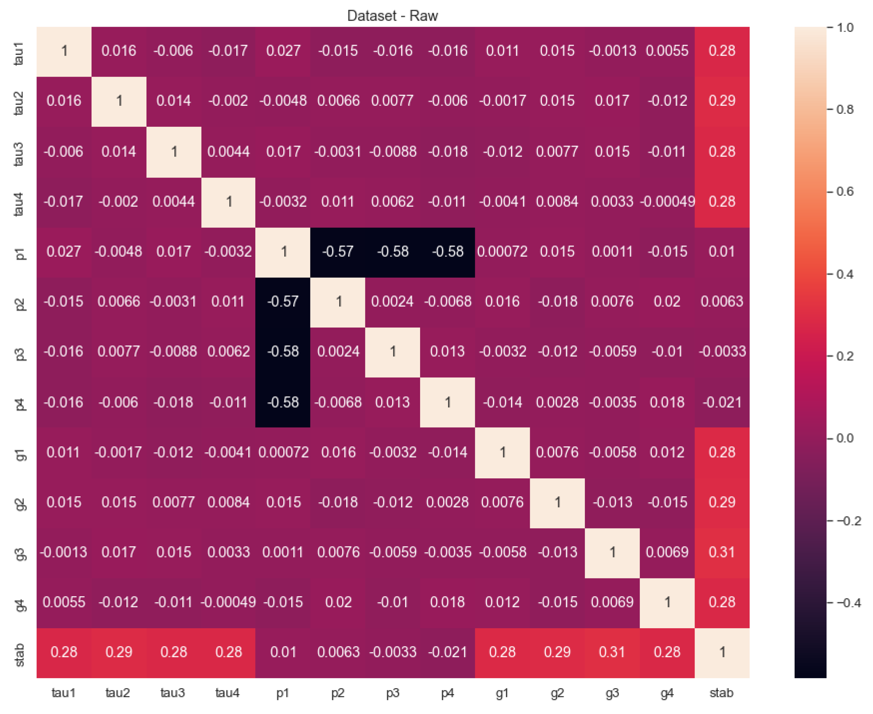
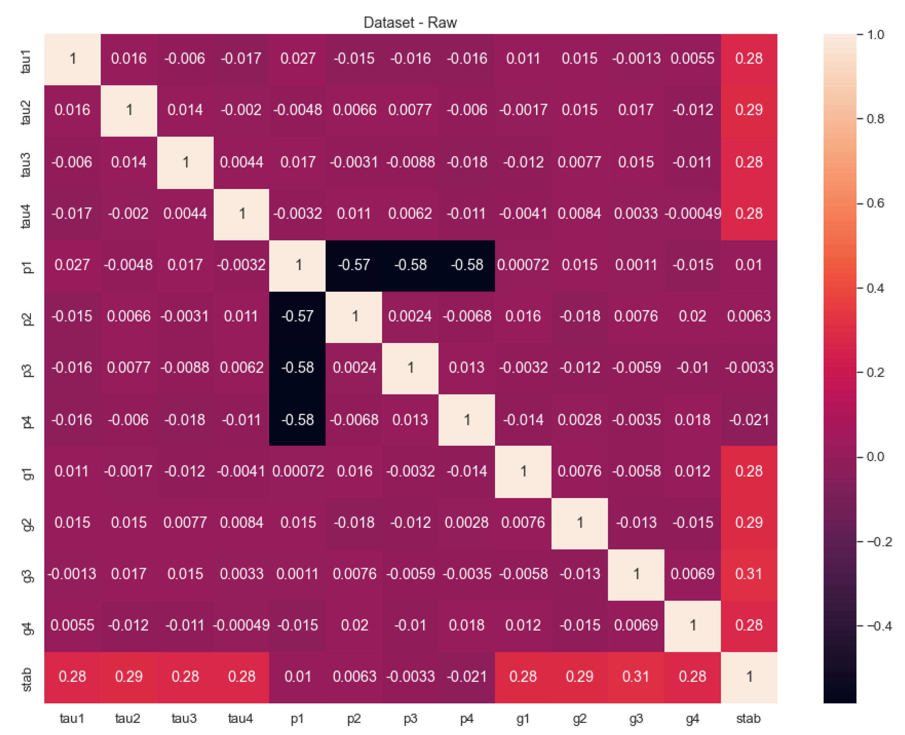
In Figure 1, we can see the correlation values of the features except for the “stabf” because it is a categorical value. However, the “stab” response figures out how it may behave in the distribution. To provide a clear understanding of Figure 1, we can investigate

Table 3. Sorted correlations of the raw dataset (ascending).

Feature Names	Correlation Values of Each Feature
p4	−0.020786
p3	−0.003321
p2	0.006255
p1	0.010278
tau1	0.275761
tau4	0.278576
g4	0.279214
tau3	0.2807
g1	0.282774
tau2	0.290975
g2	0.293601
g3	0.308235

with sorted values of the correlation values. As the correlation values point outs, the most relevant three features with the “stab” are g3, g2, and tau2. The ongoing feature importance analyses will show these values proofs in the next sections.

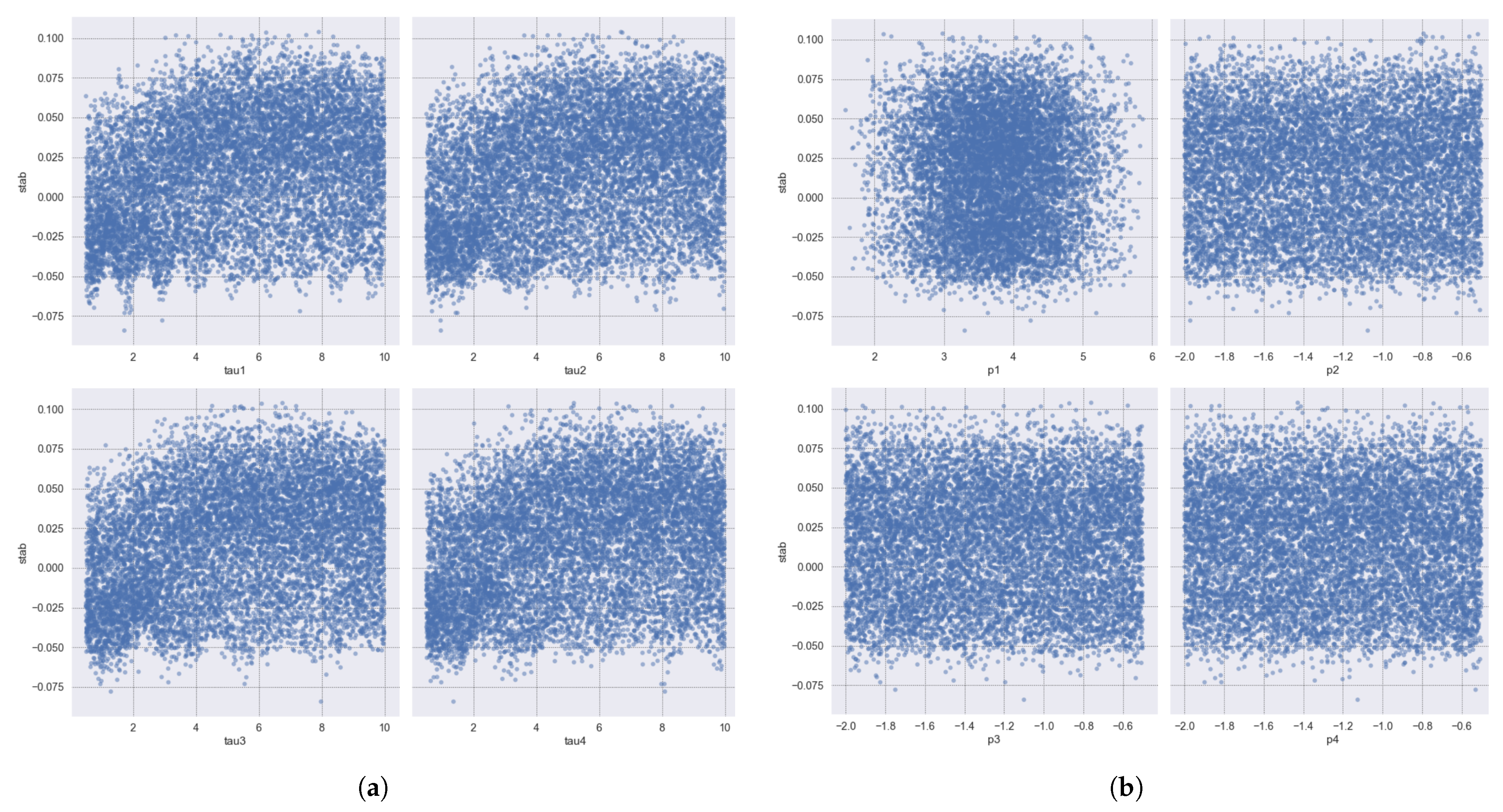
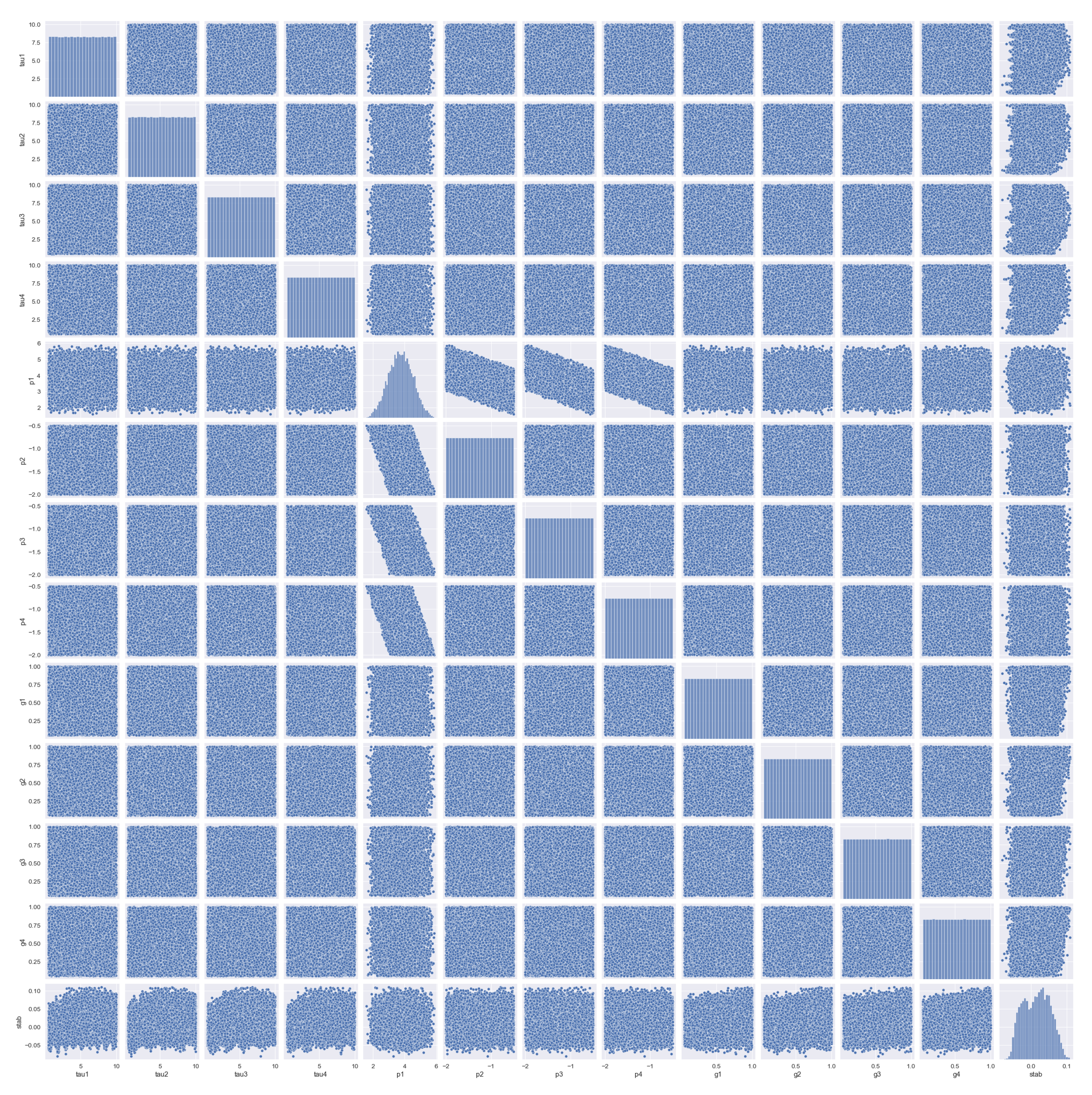
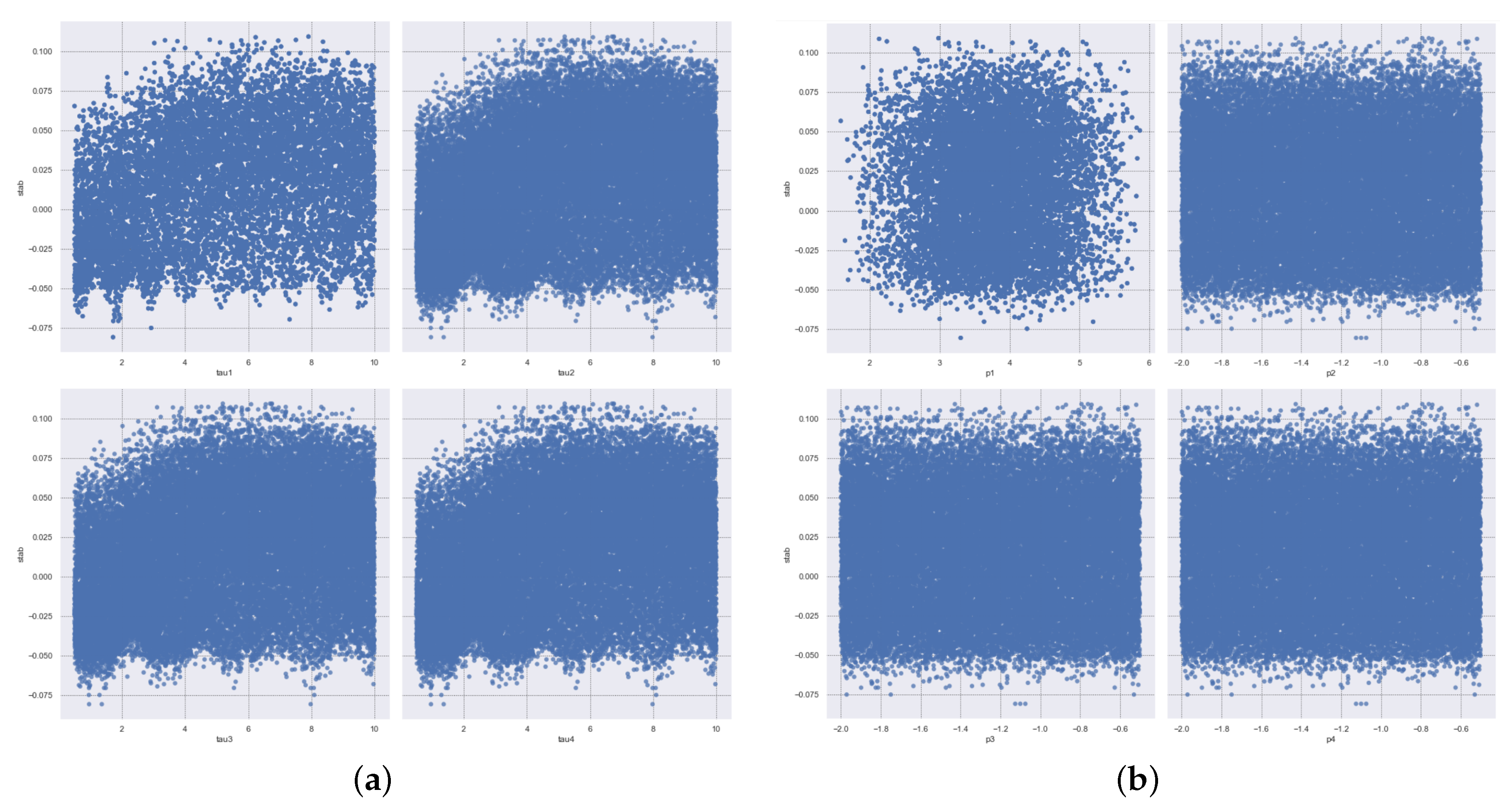
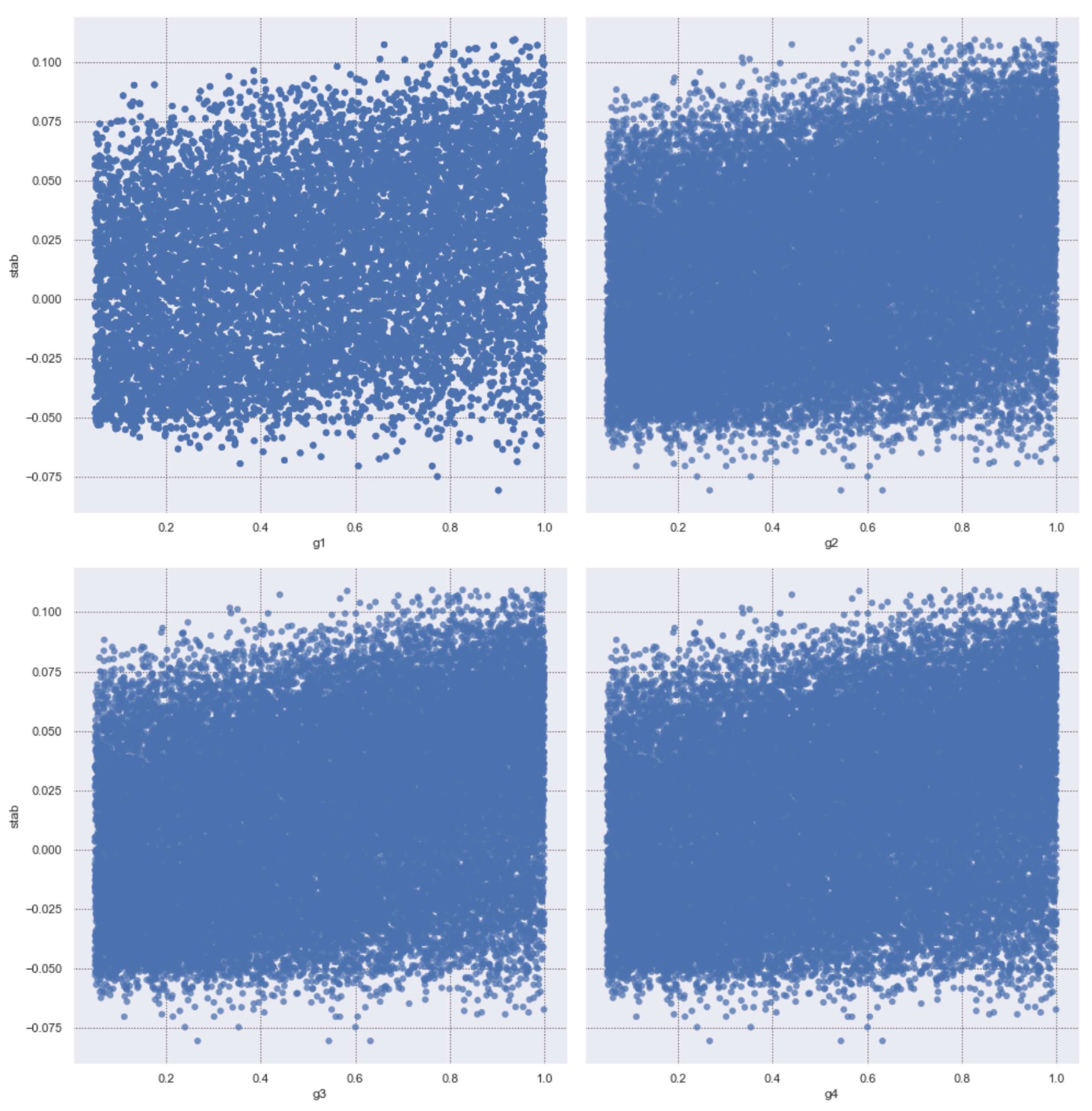
Figure 2 shows the partial scatter plots belonging to tau and p features. Here, we can see the difference in p1 distribution clearly, and also the relation of tau features has a more uniform distribution. Figure 3 demonstrates the overall scatter matrix of the raw dataset with all the features and the “stab” response. In this $13\times 13$ matrix, we can figure out the difference of the p features’ distribution clearly. Moreover, the scatter matrix shows the “stab” vs. g features scatter at the bottom line of it. Again we can realize here the most correlated features by seeing the difference in scatters.

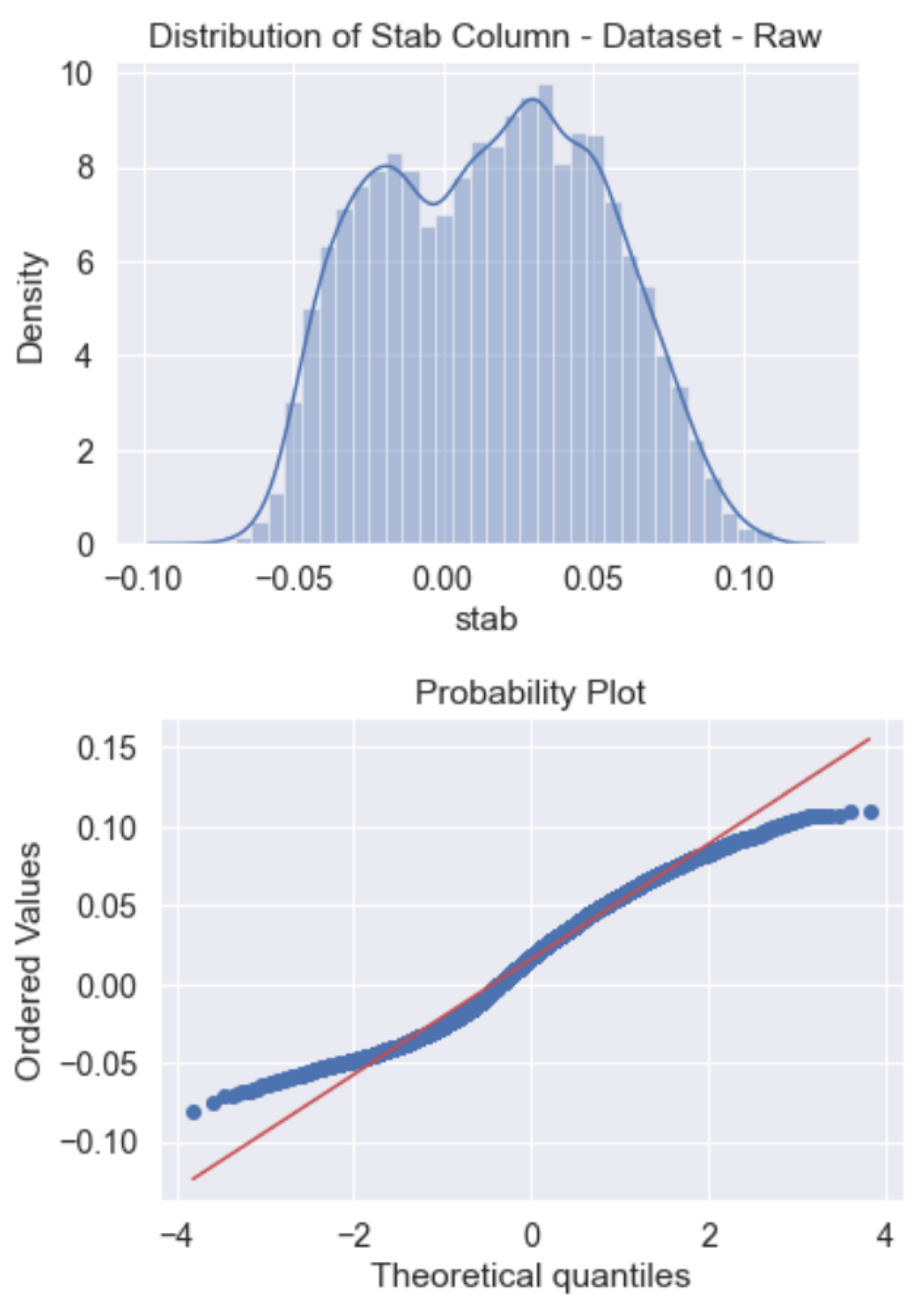
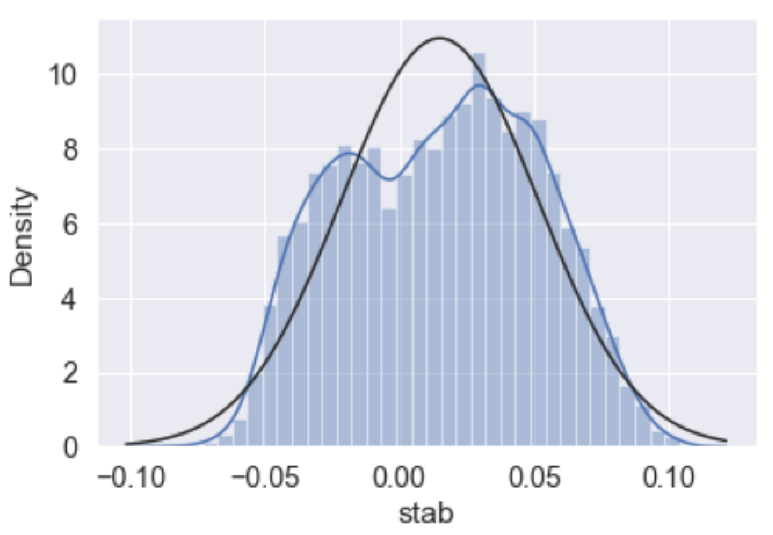
Figure 4 includes the probability plot and overall distribution of the “stab” response. We can see here the response exhibits an almost linear distribution. Additionally, in Figure 5, a distribution graph along with a normal distribution demonstration is also provided to clear out how close the “stab” response is to normal distribution.

2.2.2. Analytics of Augmented (60K) Dataset

Now, starting the data analytics of the augmented (aug) dataset,

Table 4. Statistical details of augmented dataset.

Features	Count	Mean	Std	Min	25%	50%	75%	Max
tau1	60,000	5.25	2.742434	0.500793	2.874892	5.250004	7.62469	9.999469
tau2	60,000	5.250001	2.742437	0.500141	2.875011	5.249981	7.624896	9.999837
tau3	60,000	5.250001	2.742437	0.500141	2.875011	5.249981	7.624896	9.999837
tau4	60,000	5.250001	2.742437	0.500141	2.875011	5.249981	7.624896	9.999837
p1	60,000	3.75	0.752129	1.58259	3.2183	3.751025	4.28242	5.864418
p2	60,000	−1.25	0.433017	−1.999945	−1.624997	−1.249996	−0.874993	−0.500025
p3	60,000	−1.25	0.433017	−1.999945	−1.624997	−1.249996	−0.874993	−0.500025
p4	60,000	−1.25	0.433017	−1.999945	−1.624997	−1.249996	−0.874993	−0.500025
g1	60,000	0.525	0.274244	0.050009	0.287521	0.525009	0.762435	0.999937
g2	60,000	0.525	0.274243	0.050028	0.287497	0.525007	0.76249	0.999982
g3	60,000	0.525	0.274243	0.050028	0.287497	0.525007	0.76249	0.999982
g4	60,000	0.525	0.274243	0.050028	0.287497	0.525007	0.76249	0.999982
stab	60,000	0.015731	0.036917	−0.08076	−0.015557	0.017142	0.044878	0.109403

shows important statistical measures. We can see the basic statistics like the mean, std, min, and max values with the distribution portions of quartile percentages. As we can see in the mean and std columns, the groups of features have nearly the same mean and std values except for the p1 feature like in the raw dataset before. Here, the p1 feature addresses the generation node and it is the sum of the other three consumer nodes. The aug dataset is also a clean dataset with seamless data features without any need for a complex pre-processing operation.

In Figure 6, we can see the correlation values of the features. To provide a clear understanding of Figure 6, we can investigate

Table 5. Sorted correlations of aug dataset (ascending).

Feature Names	Correlation Values of the Each Feature
p4	−0.005951
p3	−0.005951
p2	−0.005951
p1	0.010278
tau1	0.275761
g1	0.282774
tau3	0.283417
tau2	0.283417
tau4	0.283417
g4	0.293684
g2	0.293684
g3	0.293684

with sorted values of the correlation values of the augmented dataset. As the correlation values point outs the most relevant four features with the “stab” are g3, g2, g4, and tau4. In the aug dataset, the effect of g features is higher than in the raw dataset. The feature importance analysis in the next sections are going to show proof of these values.

Figure 7 shows the partial scatter plots belonging to tau and p features of the aug dataset. Here, we can see the difference in p1 distribution more clearly, and also the relation of tau features has a more uniform distribution in the augmented dataset. Figure 8 shows the scatter plots of g features a reference to the “stab” response in particular. Here we can see a more uniform distribution of g.

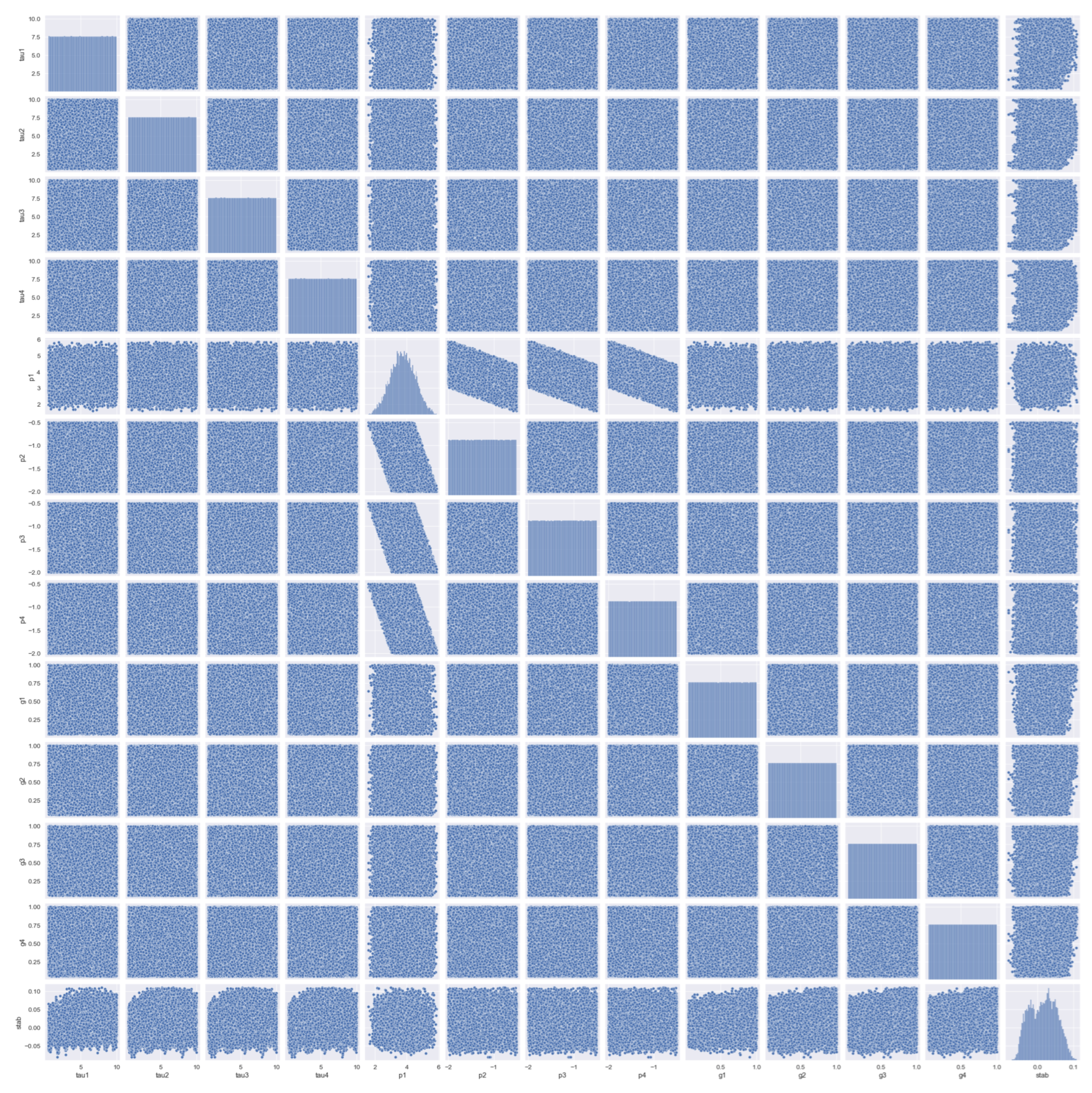
Figure 9 demonstrates the overall scatter matrix of the aug dataset with all the features and the “stab” response. In this $13\times 13$ matrix again, we can figure out the difference of the p–features’ distribution clearly. In the augmented dataset, again we can realize here the most correlated features by seeing the difference in scatters. Regarding the resolution and pixel values of the graphical presentations being very high, please feel free to zoom in to have a better vision of the visualizations.

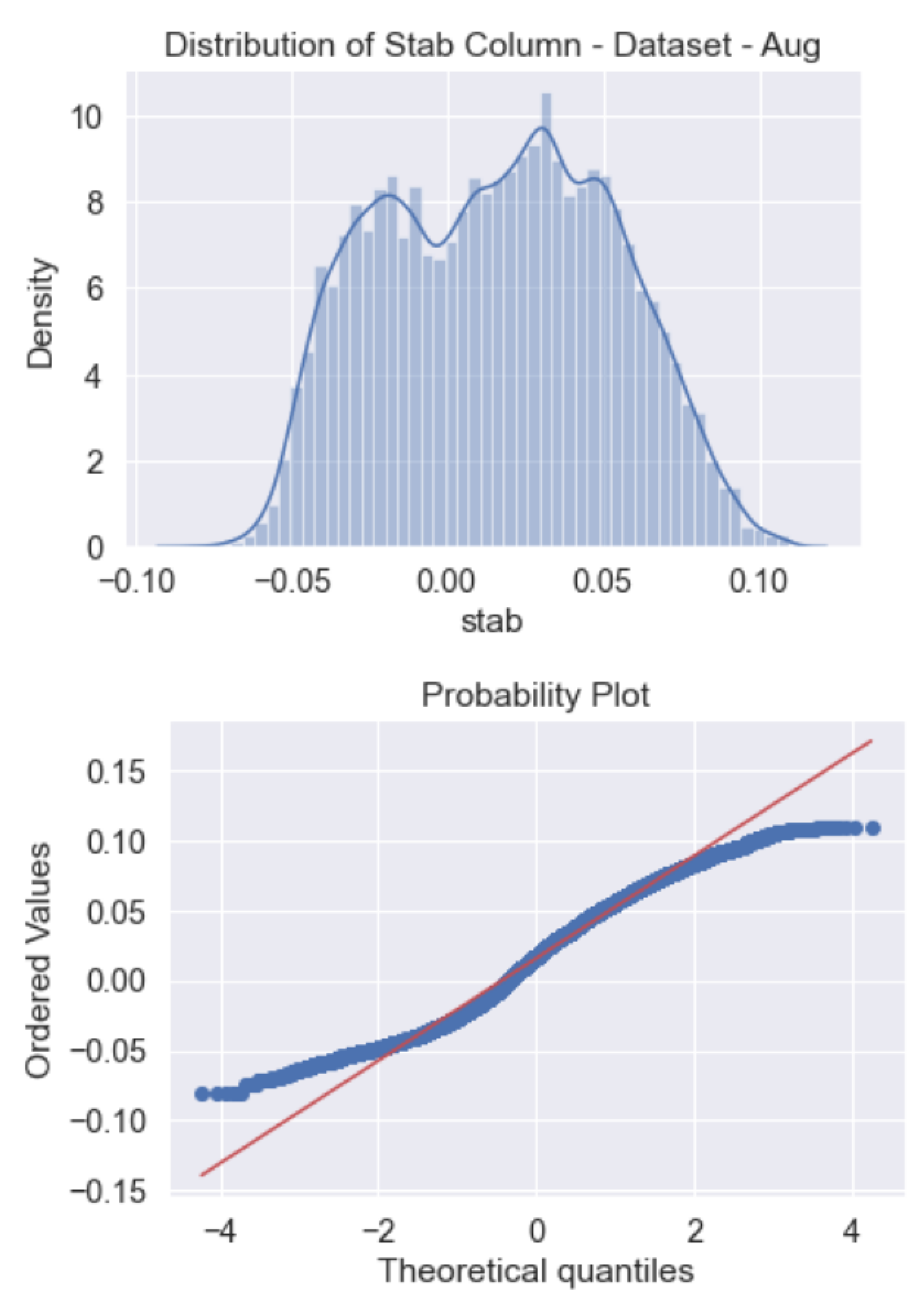
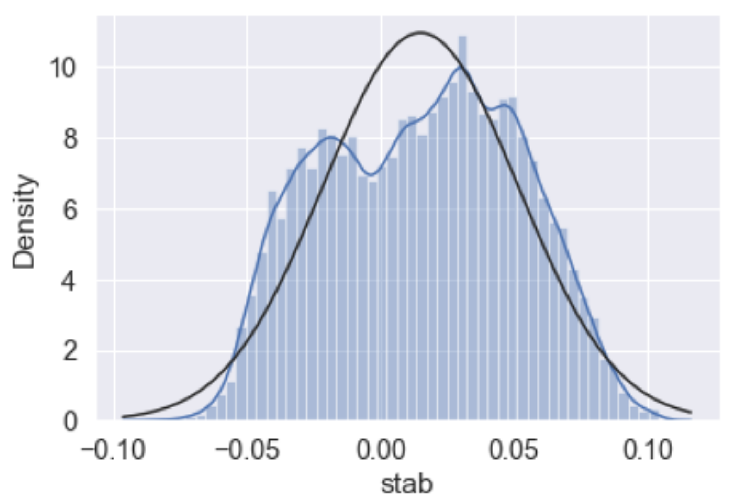
Figure 10 includes the probability plot and overall distribution of the “stab” response of the augmented dataset. We can see here again the response exhibits an almost linear distribution for the aug dataset. Additionally, in Figure 11, a distribution graph along with a normal distribution demonstration is also provided to clear out how close the “stab” response is to normal distribution. This time the response is closer to the normal distribution than the raw dataset. The excessive sample size of 60,000 may lead to this assumption. The gathered analysis reports from the data analytics and feature engineering might open a door to a better understanding of the feature importance analysis, which will be held in the next sections.

2.3. Artificial Intelligence Models

2.3.1. Gradient Boosting Machine

Gradient Boosting Machine (GBM) is a decision tree-based ensemble method with a forward learning methodology to implement its theory in regression and classification problems. In modern machine learning (ML), algorithm development goes deeply through fast and effective deployment processes, embedding the algorithm into devices in real life. Thus, there is a need to increase the refined approximations to get more accurate prediction results with heuristic guidance. GBM aims these with its effective structured design. In the proposed model, the designed GBM strategy is supported with built regression and classification trees on all the attributes of the preferred datasets in a fully distributed way, i.e., all the trees are designed and built in the way of parallel logic. Although its theoretical background is based on the study Freidman [20] and Hastie et al. [21] published many years ago in 2001 and 2004, GBM is a modern ML algorithm that has been used with increasing efficiency today.

In GBM, the trees are designed as base learners for regression or classification and exist sequentially to increase the algorithm performance. Friedman extended the GBM logic from classification to regression task [20,21]. In each iteration, GBM handles the error of the previous ensemble tree, and during the prediction process of the next tree, it deals with healing this error. Consequently, the rest of the tree ensembles are being faced with a decreasing error constantly [22].

GBM algorithm is also based on the boosting concept in which combinations of a number of models having low variance and high bias values for minimizing the high bias whilst preserving the low variance. For a clearer explanation, this means that GBM consolidates a number of shallow trees to increase the prediction or classification performance [22]. The main part that makes the difference over the boosting methods in the optimization phenomenon in classical ML algorithms is holding the optimization in function space. Because of this in GBM, $\widehat{f}$ (function estimate) is parameterized as an additional functional form as in (1) [23]:

$$\widehat{f}\left(x\right)={\widehat{f}}^L\left(x\right)=\sum _{i=0}^L{\widehat{f}}_i\left(x\right)$$

(1)

where, L is the iteration number, $\widehat{f_0}$ states the initial assumption, and the “boosts” ${\left\{\widehat{f}\right\}}_{i=1}^L$ which we can also name it increments of function [23].

GBM method includes the “base-learner” functions which we can parameterize as $h(x,\theta )$ to provide a separate definition away from function estimations of overall ensembles $\widehat{f}\left(x\right)$. Then, the formulation of the “greedy stagewise” approach for the increment of the functions can be given to base learners. To provide this formulation, the optimal step size needed to be defined in every iteration. The optimization is ruled by the formula stated in (2) and (3), to calculate the function estimations of iteration t for every N samples [23]:

$${\widehat{f}}_t\leftarrow {\widehat{f}}_{t-1}+{\rho }_{t}h(x,\theta {}_t)$$

(2)

$$({\rho }_t,{\theta }_t)=\underset{\rho ,\theta }{\mathrm{argmin}}\sum _{i=1}^N\mathsf{\Psi }(y_i,{\widehat{f}}_{t-1})+\rho h(x_i,\theta )$$

(3)

In the practical application of the GBM, it is a challenging process to obtain the base-learner function $h(x,\theta )$ properly. To deal with this obstacle, it was suggested to design the new function as being correlative to the negative gradient definition ${\left\{g_t\left(x_i\right)\right\}}_{i=1}^N$ using the observed data:

$$g_t\left(x\right)=E_y{\left[\frac{\partial \mathsf{\Psi }(y,f(x\left)\right)}{\partial f\left(x\right)}|x\right]}_{f\left(x\right)={\widehat{f}}^{t-1}\left(x\right)}$$

(4)

As an end game, the overall formulation of the GBM algorithm can be presented as a complete form whose original definition is existed in Friedman’s article [20]. At the end of the day, the whole form of the ensured algorithm, of which all the related formulations, is strongly tied to the designing of $\mathsf{\Psi }(y,f)$ and $h(x,\theta )$. Algorithm 1 briefs the whole process of GBM in pseudo-code lines. The reader can refer to studies [20,23] for a detailed explanation of the GBM phenomenon.

Algorithm 1 Gradient Boosting Machine Algorithm—Friedman’s approach

Require: 1: inputs ←${(x,y)}_{i=1}^N$ 2: iteration number ←L 3: loss-function ←$\mathsf{\Psi }=(y,f)$ 4: the model of base learner ←$h(x,\theta )$ Ensure:$\widehat{f_t}$ 5: $\widehat{f_0}$← initialization with a constant 6: for$t=1$ to L do 7:     calculation of the negative gradient $g_t\left(x\right)$ 8:     fitting the new base-learner func. $h(x,\theta {}_t)$ 9:     finding the step-size of best gradient descent ${\rho }_t$: 10:     ${\rho }_t=\underset{\rho }{\mathrm{argmin}}{\sum }_{i=1}^N\mathsf{\Psi }\left[y_i,{\widehat{f}}_{t-1}\left(x_i\right)+\rho h(x_i,\theta {}_t)\right]$ 11:     function estimate updating: 12:     ${\widehat{f}}_t\leftarrow {\widehat{f}}_{t-1}+{\rho }_{t}h(x,\theta {}_t)$ 13: end for

2.3.2. Deep Learning Model

In the modern era of scientific studies, researchers in various fields have focused on machine learning and DL interactions with their disciplines [24,25]. This trend occurs because DL algorithms go so fast into the emerging areas avoiding the handcrafted feature extraction, and easily dealing with the big data process of which classic ML algorithms collapse [26,27]. In the studies which handle the electricity data to analyze forecasting the electricity generation and consumption, there are various types of adapted ML models to obtain better performances. Among all those bunches of ML models, DL-based intelligent models have an important role in SG signal processing [28]. Since the main course of this study is not based on a pure DL model, it is avoided the detailed explanations of basic DL models to prevent any confusion in the readers’ minds. Figure 12 shows a basic DL model with $[12,10,10,1]$ layer design. The architecture details of the DL model of this study will be detailed in the experiments [10].

Before jumping into the experiments and results, we can see the evaluation metrics for the experiments of the proposed study below. Here, both the classification and regression metrics are formulated.

2.3.3. Evaluation Metrics for Classification Approach

In this study, the well-known performance metrics that suit the aim of our study are determined as accuracy (acc), precision (prec), recall or sensitivity (rec), F1-score, specificity (spec), area under the ROC curve (AUC), and Gini coefficient (2×AUC$-1$). Those metrics could draw a general picture in the readers’ minds on the way of assessment of the proposed classification models. For the enhanced explanations and other details of the preferred evaluation metrics, please refer to studies [10,29]. The Equations (5)–(9) give the formulation of the classification metrics in terms of the confusion matrix elements true positive (TP), true negative (TN), false positive (FP), and false-negative (FN):

$$\mathrm{acc}=\frac{TP+TN}{TP+TN+FP+FN}$$

(5)

$$\mathrm{prec}=\frac{TP}{TP+FP}$$

(6)

$$\mathrm{rec}=\frac{TP}{TP+FN}$$

(7)

$$\mathrm{F}1-\mathrm{score}=2\times \frac{\mathrm{prec}\times \mathrm{rec}}{\mathrm{prec}+\mathrm{rec}}=\frac{2TP}{2TP+FP+FN}$$

(8)

$$\mathrm{spec}=\frac{TN}{TN+FP}$$

(9)

2.3.4. Evaluation Metrics for Regression Approach

When it comes to the assessment of a regression model, there are fewer metrics that can fit the performance. Most of the evaluation metrics in a regression problem focus on errors between the observations and the predicted values. Moreover, to reveal a clearer understanding of how close the prediction values track the actual or observed values, there is an effective correlation metric called r-squared ($R^2$). In this study, root-mean-square errors (RMSE), mean absolute error (MAE), and $R^2$ have been taken into consideration. In the following equations, the mathematical definitions of the selected metrics are stated [15]:

$$\mathrm{MAE}=\frac{1}{n}{\displaystyle \sum _{i=0}^{n-1}}|y_i-\widehat{y_i}|$$

(10)

$$\mathrm{RMSE}=\sqrt{\frac{1}{n}\left(\sum _{i=0}^{n-1}{(y_i-\widehat{y_i})}^2\right)}$$

(11)

$$R^2=1-\frac{{\sum }_{i=1}^n{(\widehat{y_i}-y_i)}^2}{{\sum }_{i=1}^n{(\overline{y_i}-y_i)}^2},\overline{y}=\sum _{i=1}^n{y}_i$$

(12)

where $y_i$ and $\widehat{y_i}$ state the actual and predicted values, respectively, and the total sample numbers are denoted by n.

3. Results and Discussion

This section presents and discusses the obtained results for SG stability prediction in two datasets of the study. In the code design, Canonical Ubuntu 20.04 operating system (OS) installed on a workstation is used. Ubuntu OS uses the Linux kernel and is based on Debian as an open-source platform. The workstation setup has an Intel Xeon CPU with E5-2620 v4 @2.10 GHz dual-core running with 32 GB of RAM and a GPU card of Nvidia Quadro M4000 8GB.

In this study, the model design was coded on a modern AI platform of H${}_2$O [30] using the development environment as Jupyter Lab [31]. The software programming is built on the H${}_2$O Python packages [32] and also the necessary Python 3.8 packages.

H${}_2$O provides rapid and effective AI and ML systems for data scientists. It makes the process cost-effective for the experiments, and with its seamless usage of the grid search algorithm, the hyper-parameters of the proposed models could be optimized automatically. Despite a training and testing split handled in the experiments, H${}_2$O uses k-fold cross-validation in its models’ training step, then chooses the best model and conducts the testing operation to finalize the validation performance metrics.

Table 6. Model parameters of classification and regression approaches.

Model	Manually Entered Parameters
GBM	number of trees: 250, depth: 6, others are optimized automatically
DL	layers-classification:$[12,50(tanh),50(tanh),1$(softmax)], epoch: 40
	layers-regression:$[12,50(ReLu),50(ReLu),1$(Linear)], epoch: 40

describes the manually entered parameters of the GBM and DL models.

3.1. Results of the Classification Approach

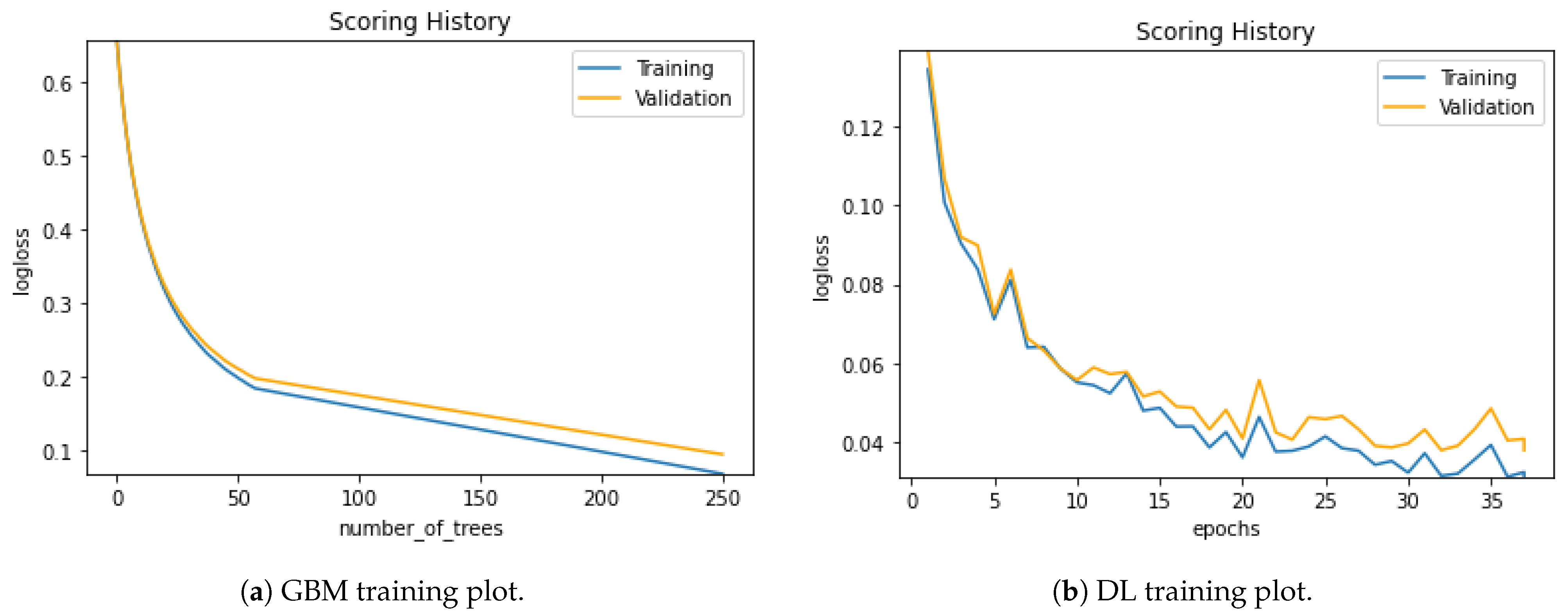
Here, the train and test ratio is used at 80% and 20% for all datasets. The readers should keep in mind that our training stage has 5-fold cross-validation, which means the proposed model has also been tested while the training stage. To give a clear presentation, the most important performance, which is the testing performance, is listed in the results tables. However, the training process can be tracked with graphical results.

Figure 13 shows the training plot of the raw dataset with GBM and DL models. Along with the training process, we can track the validation curves, too. In both models, we can see a clear training process with fewer validation and training loss errors.

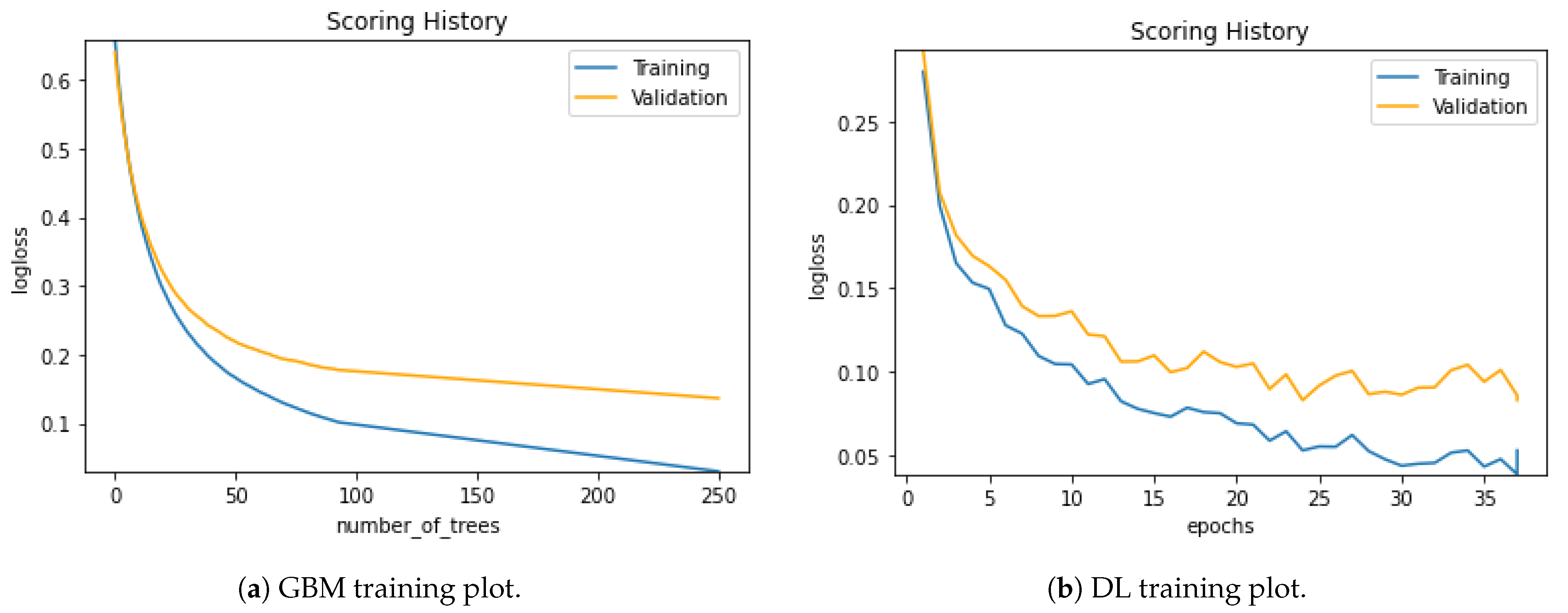
Figure 14 visualizes the training plot of the augmented dataset for the proposed models of GBM and DL.

Considering the two datasets, the training process of aug dataset runs more smoothly than the raw dataset. The validation and training loss errors in the DL model of the augmented dataset are considerably less than in the raw dataset. If we focus on the GBM model for the two datasets handled, we can see the differences in the training stages of aug and raw ones. Again, we can interpret that the loss values of the aug dataset are less than the raw datasets. The excessive sample number of the augmented dataset might be an explanation for the loss of values.

In

Table 7. Testing performances of classification approach for both models.

Evaluation Metrics	Dataset–Raw	Dataset–Aug
GBM Model
acc	0.950076	0.974814
prec	1.000000	1.000000
rec	1.000000	1.000000
F1-score	0.962279	0.980341
spec	1.000000	1.000000
AUC	0.988	0.999
Gini	0.976	0.995
DL model
Evaluation Metrics	Dataset–Raw	Dataset–Aug
acc	0.964850	0.985489
prec	1.000000	1.000000
rec	1.000000	1.000000
F1-score	0.973533	0.988692
spec	1.000000	1.000000
AUC	0.996	0.999
Gini	0.991	0.998

, we can investigate the testing results of both raw and aug datasets with related performance values produced by GBM and DL models. Here, we can interpret that the prec, spec, and rec values reached the perfect classification performance value. The AUC and Gini metrics are also high values for a classifier dealing with such a complex problem. In Table 7, we can see the acc metrics lay a bit behind according to the other metrics set. However, if we consider our datasets to have an imbalanced structure, this result is very acceptable. As it is very known, the accuracy metric does not have so many important roles in such datasets. The other specific metrics as AUC, F1-score, prec, sec, and rec metrics are more valuable compared to acc metric.

Table 8. Confusion matrix in table form.

GBM Model
	Dataset–Raw				Dataset–Aug
	stable	unstable	Error	Rate	stable	unstable	Error	Rate
stable	615	47	0.071	(47/662)	4159	137	0.0319	(137/4296)
unstable	51	1250	0.0392	(51/1301)	165	7530	0.0214	(165/7695)
Total	666	1297	0.0499	(98/1963)	4324	7667	0.0252	(302/11991)
DL model
	Dataset–Raw				Dataset–Aug
	stable	unstable	Error	Rate	stable	unstable	Error	Rate
stable	625	37	0.0559	(37/662)	4210	86	0.02	(86/4296)
unstable	32	1269	0.0246	(32/1301)	88	7607	0.0114	(88/7695)
Total	657	1306	0.0352	(69/1963)	4298	7693	0.0145	(174/11991)

includes the confusion matrix demonstrations of the proposed classifier models in our study. Here, we can select the confusion matrix values as listed in table form. By interpreting Table 8, it is clearly seen that the misclassification values of the models are very acceptable. Here, we can see the clear difference in the error rates of the raw dataset and aug dataset. While the aug dataset has an excessive number of samples, it has lower error rates than the raw dataset. This points out that the augmentation process has a positive effect on the SG stability prediction process. Moreover, it is clearly seen that the DL model has produced fewer error rates than the GBM model in both dataset performance results. The confusion matrix demonstration, which is presented by Table 8, is a good sign for the performance values of a classifier and the proposed models have valuable confusion matrix performance values.

3.2. Results of the Regression Approach

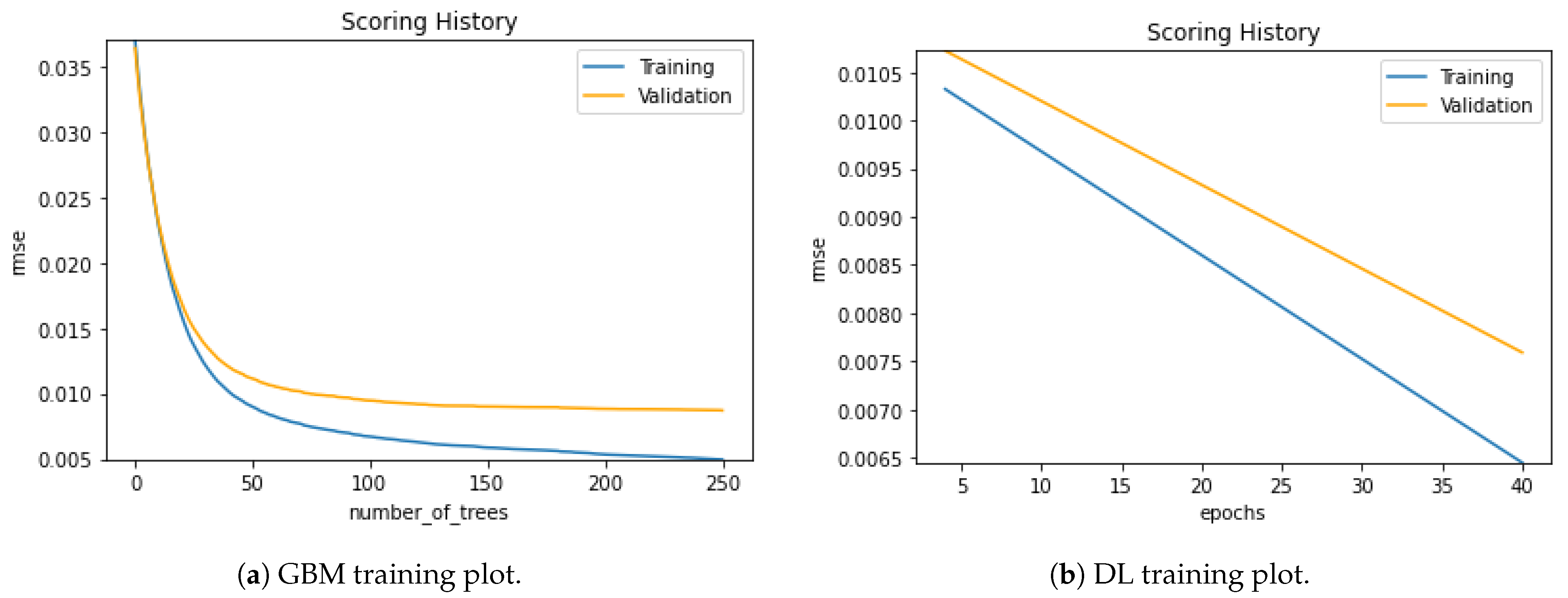
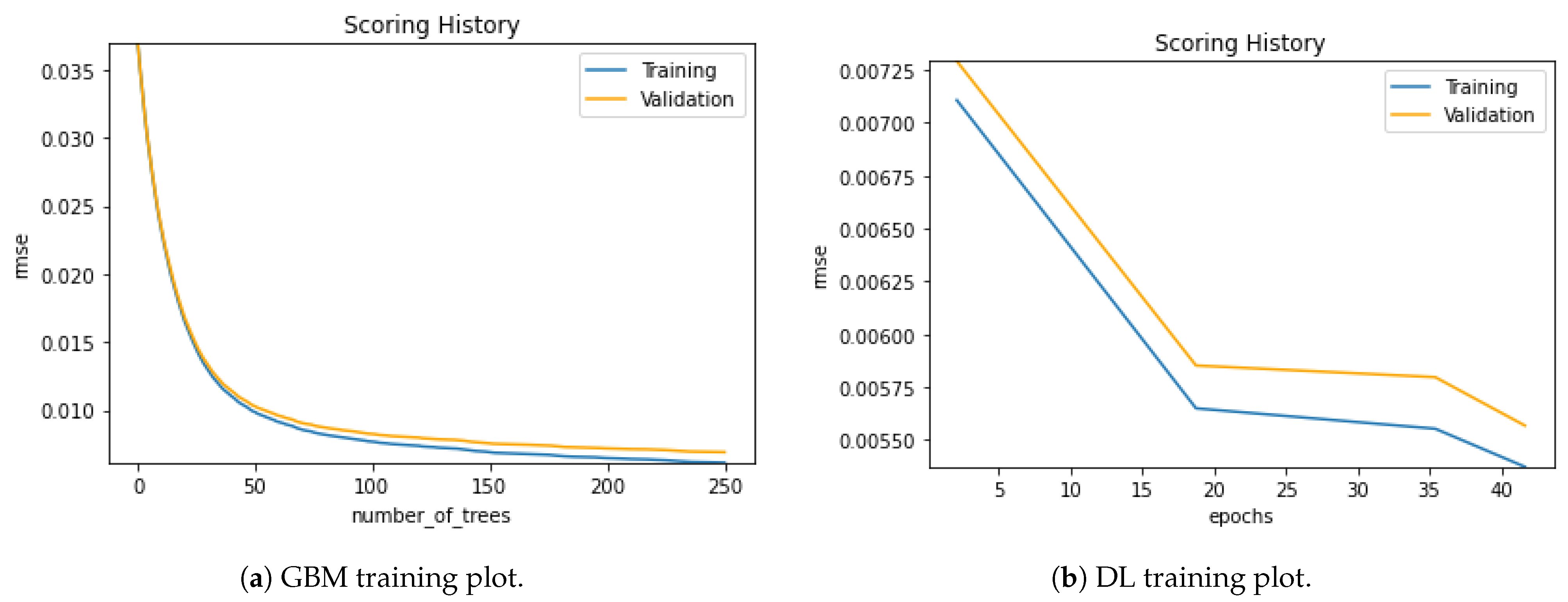
Figure 15 shows the training plot of the raw dataset with GBM and DL models for the regression approach. Together with the training process, we can follow the validation curves. In both models, we can see a clear training process with fewer validation and training loss errors.

Figure 16 visualizes the training plot of the augmented dataset for the proposed models of GBM and DL for the regression approach.

Considering the two datasets, the training process of aug dataset in the regression runs more smoothly than the raw dataset. The validation and training loss errors in the DL model of the augmented dataset are considerably less than in the raw dataset. If we look into the GBM model curves for the two datasets considered, we can see the differences in the training stages of aug and raw ones. Again, we can state that the loss values of the aug dataset are less than the raw datasets’ in the regression approach. The excessive sample number of the augmented dataset might be an explanation for the loss of values.

In

Table 9. Testing performances of regression approach for both models.

Evaluation Metrics	Dataset–Raw	Dataset–Aug
GBM model
MAE	0.006	0.005
RMSE	0.008	0.007
$R^2$	0.94	0.95
DL model
Evaluation Metrics	Dataset–Raw	Dataset–Aug
MAE	0.005	0.003
RMSE	0.006	0.005
$R^2$	0.96	0.98

, we can see the testing results of both raw and aug datasets with related performance values produced by GBM and DL models in the regression approach. Here, we can state that the MAE, RMSE, and $R^2$ values reached high values. This means that the proposed models for SG stability prediction can handle the problem effectively with the regression approach, too. Similar to the classification approach, the valuable performance metrics reached high values in regression, too. In the regression approach, the correlation-related metric r-square is the most important metric when interpreting the regression results. Here, we can see high values of the r-square in the proposed regression models.

3.3. Explainable AI-Demonstration for Classification

As it is mentioned before, this study includes comprehensive analyses of the SG stability datasets used in the literature. This part of the article, there given the results of the classification and regression models. In this sub-section, it is time to present the explainable AI (XAI) analysis results. In the following analyses of XAI, the graphical results of the proposed classification model GBM are considered. Because the main course of this study is based on the state-of-the-art GBM model for the SG stability prediction in a classification manner. The XAI analyses are handled on some detailed feature analysis to make clear the model understanding with proofs.

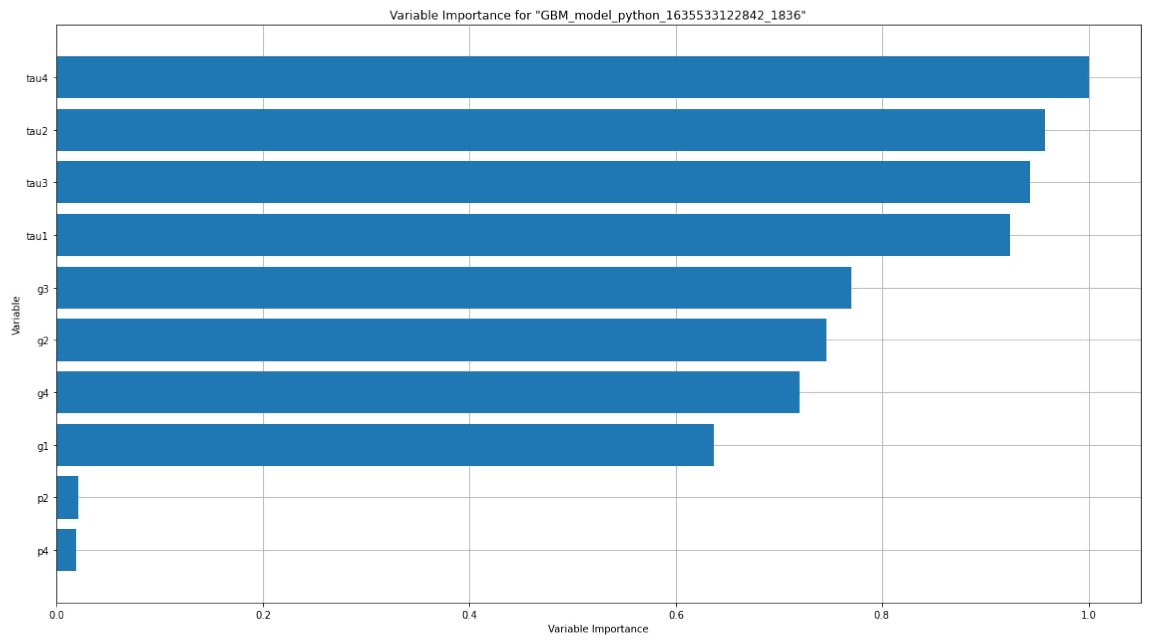
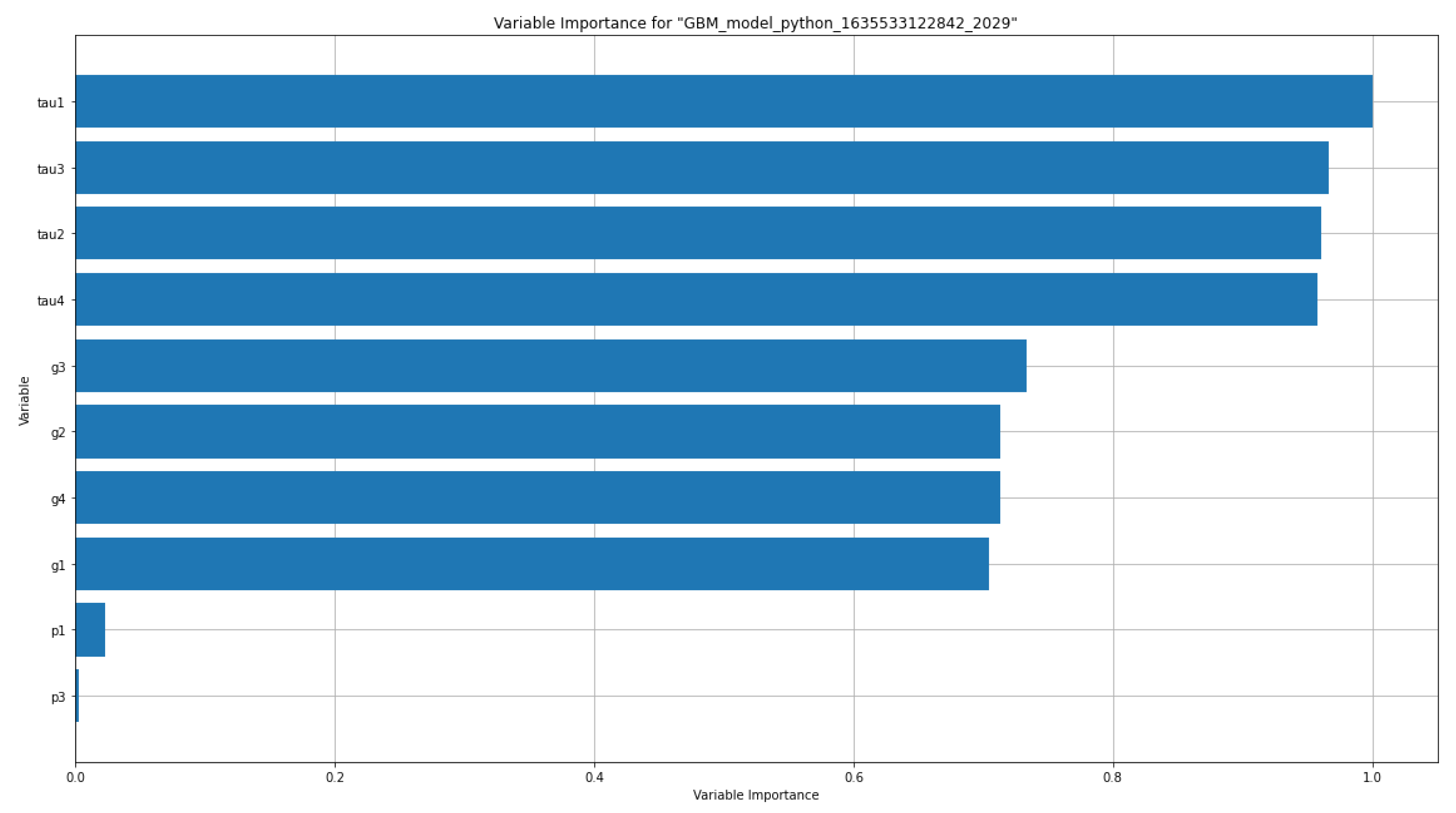
Firstly, the variable importance graphics are demonstrated. The variable importance graphic states the relative importance of the most important variables in the models. As it is mentioned before in the feature correlation matrices, we can see that the highly correlated features with the response “stab” takes to the front here, too. Figure 17 and Figure 18 show the detailed bar graphs of variable importance values of the raw dataset and aug dataset for the proposed GBM model, respectively.

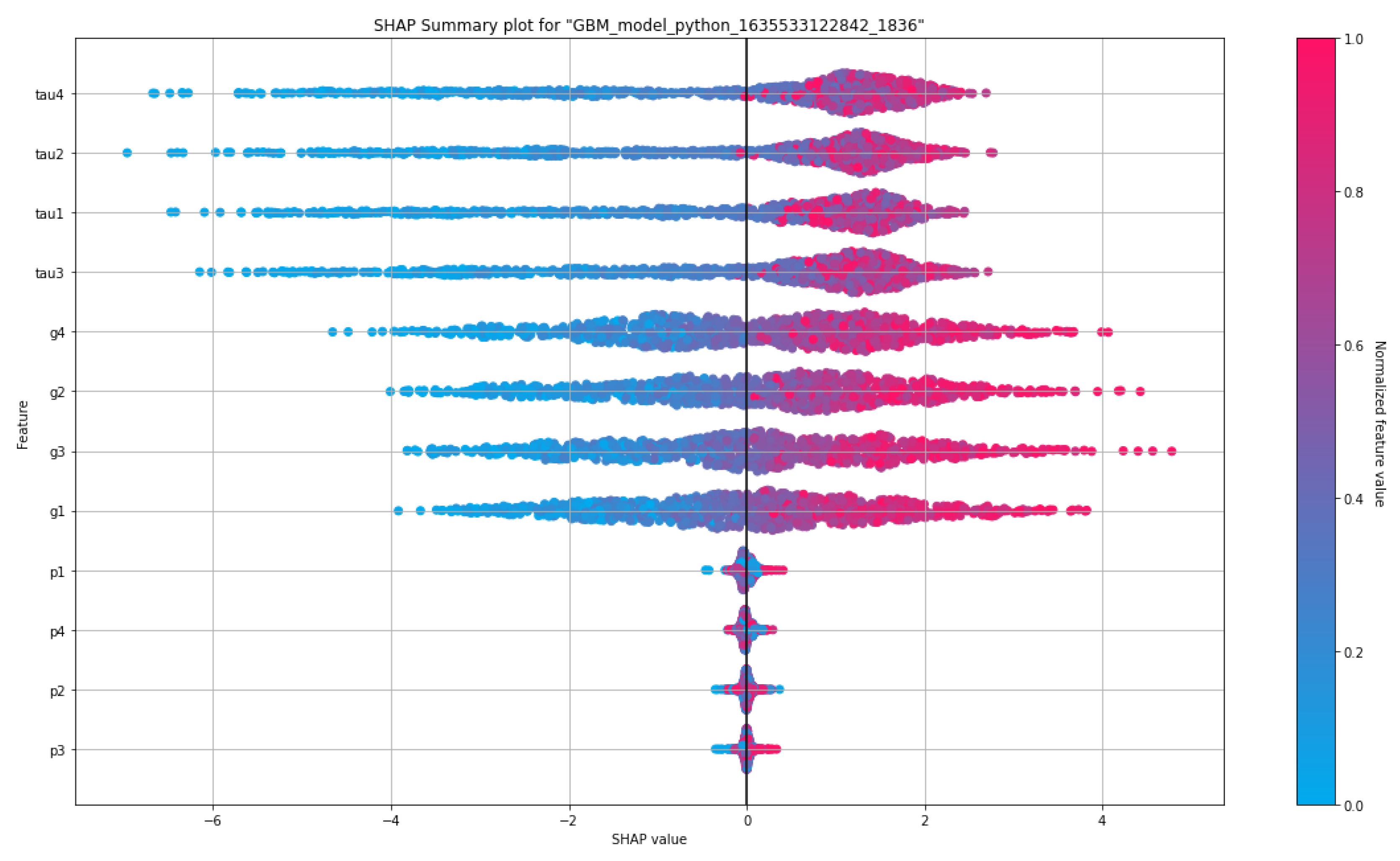
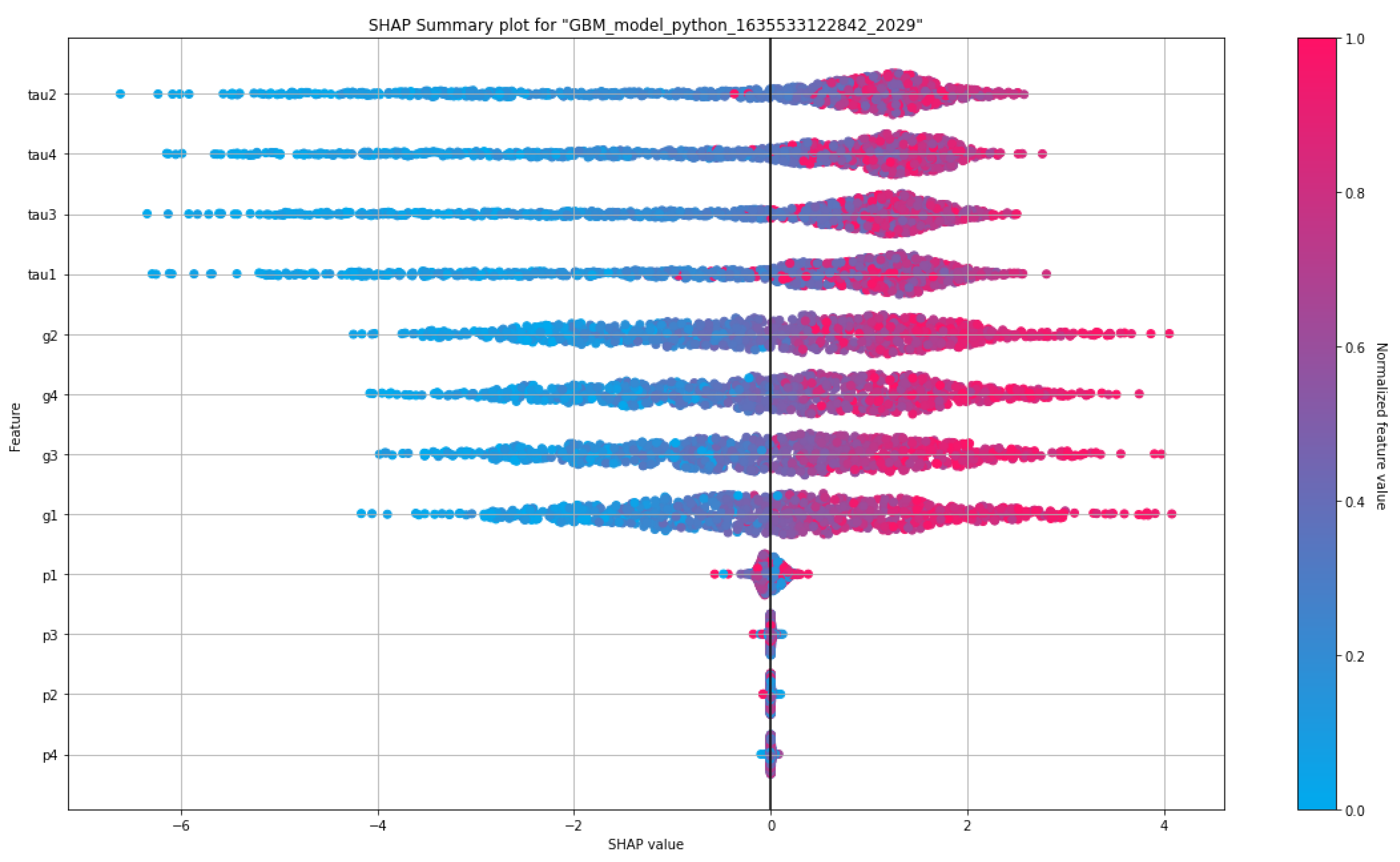
SHapley Additive exPlanations (SHAP) summary graphics visualize the contribution of the features for each row of the dataset. The main purpose of SHAP is to describe the prediction of a sample of the dataset by computing the contribution for each feature to values of the prediction [30]. The SHAP plot can further state the positive or negative relationships of the features with the response variables. Figure 19 and Figure 20 show the SHAP plots of the proposed GBM model for the raw and augmented datasets, respectively. Here, our SHAP plots tell that the p–features contribute to the response less than other features. Apparently, there would be conducted any additional analyses with dropping the p–features from both datasets. These assumptions clearly sensed from the correlation matrices and variable importance plots, too. The dominance behavior of the g and tau features are clearly seen with the SHAP plots.

As an additional comment, we can say that contribution of the p–features to the classification response is very less in the augmented dataset. The power effect in the grid should be examined in accordance with the whole behavior of the SG. As generally speaking on the SHAP plots presented in Figure 19 and Figure 20, both the augmented dataset and raw dataset have the same features which are much confronting in the whole distribution.

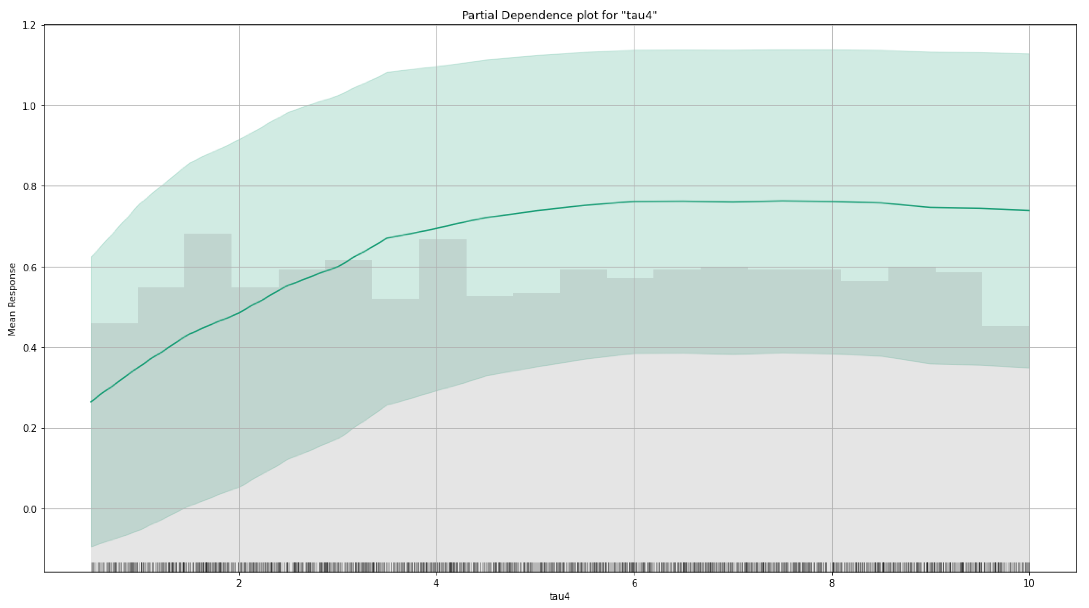
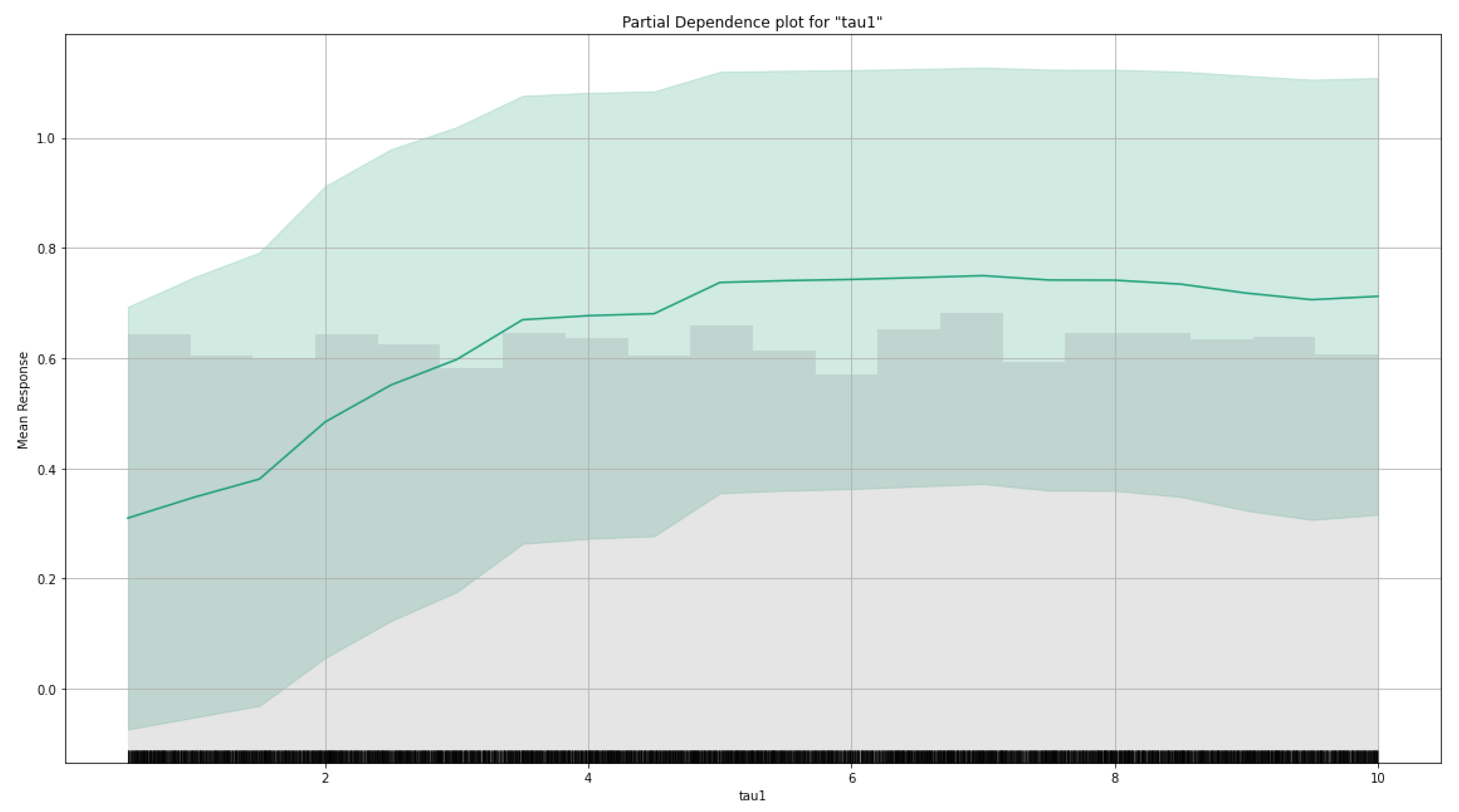
Figure 21 and Figure 22 demonstrate the partial dependence graphs of the proposed GBM model for the raw and the aug datasets, respectively. These plots are presented only for the tau4 in the raw dataset and tau1 in the augmented dataset. Because these features are at the top of the variable importance list for the raw and aug datasets. A partial dependence plot (PDP) shows a graphical visualization of the marginal effect of a feature on the response. The effect of a feature can be measured in variation in the mean values of the responses. PDP states the independence between the feature for the one it is the PDP calculated and the remains [30].

Here in PDP visualizations, we can interpret that the value of the most relevant features directly affects the SG stability. However, both in the raw dataset and aug dataset, we can say that after a specific value (at about the value of 6) of the tau features, the stability is not affected anymore.

3.4. The Overall Comparison of the Results with the Existing Studies in the Literature

The final part of the results and discussion section ends with a general comparison. As mentioned before, we collected all the studies that used the same dataset in the related literature on SG stability prediction. In

Table 10. Studies in the literature using the same datasets of SG stability prediction.

Study	Year	Dataset	Approach	Model
This study	2021	Augmented and Raw	Classification and Regression	GBM
[10]	2021	Augmented	Classification	DL
[13]	2021	Raw	Classification	Decision Tree
[14]	2021	Raw	Classification	Decision Tree
[15]	2021	Raw	Regression	BiGRU
[16]	2021	Augmented	Classification	CNN
[12]	2020	Raw	Classification	LSTM
[11]	2019	Raw	Classification	ML
[5]	2018	Raw	Classification	Decision Tree

, all the studies focusing on SG stability prediction are integrated. As seen in Table 10, most of the studies handled the SG stability problem as a classification approach and preferred the raw dataset. Only this study, the preliminary study of this study’s author [16], and study [10] considered the augmented dataset in the process. Moreover, a conference proceeding [15] attempted to handle the problem as a regression approach.

To picture an overall comparison,

Table 11. Performance comparisons.

Study	Acc	F1-Score	${\mathit{R}}^2$
This Study	0.97	1.000	0.96
[10]	0.99	0.99	-
[13]	0.97	0.97	-
[14]	0.99	-	-
[15]	-	-	0.97
[16]	0.99	0.98	-
[12]	0.99	-	-
[11]	0.91	0.91	-
[5]	-	-	-

is provided. Here the proper evaluation metrics are integrated to shape a fair comparison scenario. Most of the studies take the acc metric in the first place, even though it is not a satisfying metric in all situations. However, in brief words, the proposed study has outperformed most of the studies existing in the literature in terms of various evaluation metrics such as the spec, rec, prec, and F1-score. When it comes to overall assessments of the existing studies, the proposed study stays in a different place, including a comprehensive analysis of feature engineering and XAI. Obtained results show that the proposed GBM method has an outstanding place in the SG stability prediction in both classification and regression approaches. The preliminary study of this article’s author, the presented abstract study [16], includes a basic CNN model and does not handle the dataset in such a comprehensive way as exists in the proposed study. In particular, when similar studies are examined in the literature which has the same purpose and includes the same dataset, it is seen that the proposed study is the first holistic study to handle the SG stability problem with classification and regression problem with such an enhanced analysis.

4. Conclusions

The excessive spread of renewable energy has some challenges along with its advantages. The distributed structure of modern times electrical grid topology required a bidirectional and symmetrical power flow in SG. Integrating all the players of the electrical grid along with the price policy determination is a process that needs to be operated seamlessly. In such a complicated process, DSGC opens a door to the solution for system management with its easy-to-access operation based on frequency. Even though DSGC can unquestionably handle the grid stability operation, it still has drawbacks, including major simplifications in its calculation nature.

In this paper, an enhanced model is proposed with the power of explainable AI and feature engineering for the prediction of SG stability. The proposed study has important points, such as taking the problem with both classification and regression manner as a symmetrical approach. Moreover, this study has a role to draw a holistic picture of the existing studies putting them on a table, and proposing a novel structure that outperforms the drawbacks of the former methods. The proposed GBM model and designed DL model have produced a prominent performance.

The GBM is a robust technique that can effectively predict complex non-linear function dependencies. The decision tree-based model family has shown significant success in various practical implementations. Furthermore, the GBMs are exceptionally resilient and can easily be adapted to different practical demands. However, all these outputs and advantages have a price. Although GBMs can be well-considered to be a methodological concept than a specific method, they still have some drawbacks.

The most remarkable problem of the GBMs that appears in practical experience is their memory consumption. Predictive model storage capacity depends on the size of boosting iterations used in the learning. Despite that, this issue with memory consumption is common to all the ensemble techniques and appears more considerably with the increased number of models to be stored.

One other problem of GBM that is naturally sourced from the high memory consumption is the evaluation speed. To operate the fitted GBM model for predictions, the user has to evaluate all of the base learners in the structure of the ensemble. Considering the simplicity of each of them, when the ensemble is noticeably large, gathering predictions at a fast pace can be time-consuming. For this reason, preferring GBMs in excessive online tasks would presumably require the user to credit a trade-off between the complexity of the model and the desired function evaluations per time sampling. Nevertheless, when the GBM is already learned, the user can draw full advantage of parallelization in obtaining the predictions.

The stated problems above are merely computational and accordingly, they can be noted the cost of having a stronger model. As we have mentioned, GBMs are extremely practicable, providing various beneficial properties to the field-operators.

Moreover, GBMs can be addressed as a scaffold for model design, in this way providing the experts the opening not only to customize but also to plan particular novel GBM models for specific tasks. This superior flexibility has led to improvement of a broad range of GBM algorithm designs. Moreover, the proposed model in this study is empowered with deep learning and XAI to provide a robust implementation.

The XAI analyses revealed important bottom lines to be considered. Moreover, the proposed study handles both SG datasets that are being researched by the related experts to date. After the results of the comprehensive analysis, future studies should be considered to combine the data analytics touch with the smart grid deeply.

References

- Saleh, A.I.; Rabie, A.H.; Abo-Al-Ez, K.M. A data mining based load forecasting strategy for smart electrical grids. Adv. Eng. Inform. 2016, 30, 422–448. [Google Scholar] [CrossRef]
- Tsaousoglou, G.; Pinson, P.; Paterakis, N.G. Transactive Energy for Flexible Prosumers Using Algorithmic Game Theory. IEEE Trans. Sustain. Energy 2021, 12, 1571–1581. [Google Scholar] [CrossRef]
- Fellah, K.; Abbou, R.; Khiat, M. Energy management system for surveillance and performance analysis of a micro-grid based on discrete event systems. Int. J. Green Energy 2021, 18, 1104–1116. [Google Scholar] [CrossRef]
- Guizani, M.; Anan, M. Smart grid opportunities and challenges of integrating renewable sources: A survey. In Proceedings of the IWCMC 2014-10th International Wireless Communications and Mobile Computing Conference, Nicosia, Cyprus, 4–8 August 2014; pp. 1098–1105. [Google Scholar] [CrossRef]
- Arzamasov, V.; Bohm, K.; Jochem, P. Towards Concise Models of Grid Stability. In Proceedings of the 2018 IEEE International Conference on Communications, Control, and Computing Technologies for Smart Grids, SmartGridComm 2018, Aalborg, Denmark, 29–31 October 2018; pp. 1–6. [Google Scholar] [CrossRef]
- Reddy, S.; Akashdeep, S.; Harshvardhan, R.; Kamath, S. Stacking Deep learning and Machine learning models for short-term energy consumption forecasting. Adv. Eng. Inform. 2022, 52, 101542. [Google Scholar]
- Siniosoglou, I.; Radoglou-Grammatikis, P.; Efstathopoulos, G.; Fouliras, P.; Sarigiannidis, P. A Unified Deep Learning Anomaly Detection and Classification Approach for Smart Grid Environments. IEEE Trans. Netw. Serv. Manag. 2021, 18, 1137–1151. [Google Scholar] [CrossRef]
- Schäfer, B.; Matthiae, M.; Timme, M.; Witthaut, D. Decentral Smart Grid Control. New J. Phys. 2015, 17, 015002. [Google Scholar] [CrossRef]
- Schäfer, B.; Grabow, C.; Auer, S.; Kurths, J.; Witthaut, D.; Timme, M. Taming instabilities in power grid networks by decentralized control. Eur. Phys. J. Spec. Top. 2016, 225, 569–582. [Google Scholar] [CrossRef] [Green Version]
- Breviglieri, P.; Erdem, T.; Eken, S. Predicting Smart Grid Stability with Optimized Deep Models. SN Comput. Sci. 2021, 2, 73. [Google Scholar] [CrossRef]
- Moldovan, D.; Salomie, I. Detection of Sources of Instability in Smart Grids Using Machine Learning Techniques. In Proceedings of the 2019 IEEE 15th International Conference on Intelligent Computer Communication and Processing, ICCP 2019, Cluj-Napoca, Romania, 5–7 September 2019; pp. 175–182. [Google Scholar] [CrossRef]
- Alazab, M.; Khan, S.; Krishnan, S.S.R.; Pham, Q.V.; Reddy, M.P.K.; Gadekallu, T.R. A Multidirectional LSTM Model for Predicting the Stability of a Smart Grid. IEEE Access 2020, 8, 85454–85463. [Google Scholar] [CrossRef]
- Li, C. Stability analysis of distributed smart grid based on machine learning. In IOP Conference Series: Earth and Environmental Science; IOP Publishing Ltd.: Bristol, UK, 2021; Volume 692, p. 022125. [Google Scholar] [CrossRef]
- Bashir, A.K.; Khan, S.; Prabadevi, B.; Deepa, N.; Alnumay, W.S.; Gadekallu, T.R.; Maddikunta, P.K.R. Comparative analysis of machine learning algorithms for prediction of smart grid stability†. Int. Trans. Electr. Energy Syst. 2021, 31, e12706. [Google Scholar] [CrossRef]
- Massaoudi, M.; Abu-Rub, H.; Refaat, S.S.; Chihi, I.; Oueslati, F.S. Accurate Smart-Grid Stability Forecasting Based on Deep Learning: Point and Interval Estimation Method. In Proceedings of the 2021 IEEE Kansas Power and Energy Conference (KPEC), Manhattan, KS, USA, 19–20 April 2021; pp. 1–6. [Google Scholar] [CrossRef]
- Ucar, F. The lightweight deep learning model for smart grid stability prediction. In Proceedings of the TUBA World Conference on Energy Science and Technology (TUBA WCEST-2021), Online, 8–12 August 2021; pp. 210–211. [Google Scholar]
- Holzinger, A.; Kieseberg, P.; Weippl, E.; Tjoa, A.M. Current advances, trends and challenges of machine learning and knowledge extraction: From machine learning to explainable AI. In Proceedings of the International Cross-Domain Conference for Machine Learning and Knowledge Extraction, Hamburg, Germany, 27–30 August 2018; Springer: Berlin/Heidelberg, Germany, 2018; pp. 1–8. [Google Scholar]
- Adadi, A.; Berrada, M. Peeking inside the black-box: A survey on explainable artificial intelligence (XAI). IEEE Access 2018, 6, 52138–52160. [Google Scholar] [CrossRef]
- Tibshirani, R.; Hastie, T. A Melting Pot. Obs. Stud. 2021, 7, 213–215. [Google Scholar] [CrossRef]
- Friedman, J.H. Greedy function approximation: A gradient boosting machine. Ann. Stat. 2001, 29, 1189–1232. [Google Scholar] [CrossRef]
- Bartlett, P.L.; Bickel, P.J.; Bühlmann, P.; Freund, Y.; Friedman, J.; Hastie, T.; Jiang, W.; Jordan, M.J.; Koltchinskii, V.; Lugosi, G.; et al. Discussions of boosting papers, and rejoinders. Ann. Stat. 2004, 32, 85–134. [Google Scholar] [CrossRef]
- Ikeagwuani, C.C. Estimation of modified expansive soil CBR with multivariate adaptive regression splines, random forest and gradient boosting machine. Innov. Infrastruct. Solut. 2021, 6, 199. [Google Scholar] [CrossRef]
- Natekin, A.; Knoll, A. Gradient boosting machines, a tutorial. Front. Neurorobotics 2013, 7, 21. [Google Scholar] [CrossRef]
- Li, Y.H.; Wu, T.X.; Zhai, D.W.; Zhao, C.H.; Zhou, Y.F.; Qin, Y.G.; Su, J.S.; Qin, H. Hybrid Decision Based on DNN and DTC for Model Predictive Torque Control of PMSM. Symmetry 2022, 14, 693. [Google Scholar] [CrossRef]
- Islamov, S.; Grigoriev, A.; Beloglazov, I.; Savchenkov, S.; Gudmestad, O.T. Research risk factors in monitoring well drilling—A case study using machine learning methods. Symmetry 2021, 13, 1293. [Google Scholar] [CrossRef]
- Akhtar, M.S.; Feng, T. Detection of Malware by Deep Learning as CNN-LSTM Machine Learning Techniques in Real Time. Symmetry 2022, 14, 2308. [Google Scholar] [CrossRef]
- Sultanbekov, R.; Beloglazov, I.; Islamov, S.; Ong, M.C. Exploring of the incompatibility of marine residual fuel: A case study using machine learning methods. Energies 2021, 14, 8422. [Google Scholar] [CrossRef]
- Alarfaj, F.K.; Khan, N.A.; Sulaiman, M.; Alomair, A.M. Application of a Machine Learning Algorithm for Evaluation of Stiff Fractional Modeling of Polytropic Gas Spheres and Electric Circuits. Symmetry 2022, 14, 2482. [Google Scholar] [CrossRef]
- Omitaomu, O.A.; Niu, H. Artificial Intelligence Techniques in Smart Grid: A Survey. Smart Cities 2021, 4, 548–568. [Google Scholar] [CrossRef]
- H2O.ai. H2O: Scalable Machine Learning Platform; Version 3.30.0.6; H2O.ai Company: New York, NY, USA, 2020. [Google Scholar]
- Kluyver, T.; Ragan-Kelley, B.; Pérez, F.; Granger, B.E.; Bussonnier, M.; Frederic, J.; Kelley, K.; Hamrick, J.B.; Grout, J.; Corlay, S.; et al. Jupyter Notebooks-a Publishing Format for Reproducible Computational Workflows; JupyterLab. IOS Press: Amsterdam, The Netherlands, 2016; Volume 2016. [Google Scholar]
- H2O.ai. H2O: Python Interface for H2O; Python Package Version 3.30.0.6; H2O.ai Company: New York, NY, USA, 2020. [Google Scholar]
Figure 1.
Correlation matrix of the raw dataset.
Figure 2.
Scatter plots of tau and p features of raw dataset depends to stab. (Please zoom in for a detailed view). (a) stab vs tau1 to tau4 features. (b) stab vs p1 to p4 features.
Figure 3.
Scatter matrix of the raw dataset.
Figure 4.
Overall distribution and probability plot of “stab” response of raw dataset.
Figure 5.
Distribution graph of “stab” response of raw dataset with normal distribution plot.
Figure 6.
Correlation matrix of the augmented dataset.
Figure 7.
Scatter matrix of the augmented dataset. (a) stab vs tau1 to tau4 features. (b) stab vs p1 to p4 features.
Figure 8.
Scatter plots of g features of aug dataset depends to stab.
Figure 9.
Scatter matrix of the augmented dataset.
Figure 10.
Overall distribution and probability plot of “stab” response of aug dataset.
Figure 11.
Distribution graph of “stab” response of aug dataset with normal distribution plot.
Figure 12.
A general architecture of a deep model.
Figure 13.
Training plots of the raw dataset for GBM and DL models.
Figure 14.
Training plots of aug dataset for GBM and DL models.
Figure 15.
Training plots of the raw dataset for GBM and DL models–regression.
Figure 16.
Training plots of aug dataset for GBM and DL models–regression.
Figure 17.
Variable importance graph of raw dataset–GBM Model.
Figure 18.
Variable importance graph of aug dataset–GBM Model.
Figure 19.
SHAP graph of raw dataset–GBM Model.
Figure 20.
SHAP graph of aug dataset–GBM Model.
Figure 21.
Partial dependence graph of tau1 in raw dataset–GBM Model.
Figure 22.
Partial dependence graph of tau1 in aug dataset–GBM Model.