Article

Discriminant Analysis Based on the Patch Length and Crack Depth to Determine the Convergence of Global–Local Non-Intrusive Analysis with 1D-to-3D Coupling

by
Matías Jaque-Zurita
1,
Jorge Hinojosa
2,
Emilio Castillo-Ibarra
1 and
Ignacio Fuenzalida-Henríquez
3,*
1
Engineering Systems Doctoral Program, Faculty of Engineering, Universidad de Talca, Campus Curicó, Curicó 3340000, Chile
2
Industrial Technologies Department, Faculty of Engineering, University of Talca, Campus Curicó, Curicó 3340000, Chile
3
Building Management and Engineering Department, Faculty of Engineering, University of Talca, Campus Curicó, Curicó 3340000, Chile
*
Author to whom correspondence should be addressed.
Symmetry 2023, 15(11), 2068; https://doi.org/10.3390/sym15112068
Submission received: 17 August 2023 / Revised: 13 October 2023 / Accepted: 18 October 2023 / Published: 15 November 2023
(This article belongs to the Special Issue Emerging Applications of Machine Learning in Smart Systems Symmetry)

Abstract

:
Reducing the time spent on computational simulations is an active area in solid mechanics, and efforts are being made to implement novel techniques and apply them to time-sensitive areas in the industry and research. One of these techniques is called global–local non-intrusive analysis, a methodology that enriches a local patch model using 3D elements with non-linear behavior (such as crack propagation), coupled with a linear, global 1D frame model that solves iteratively, thereby reducing overall times compared to a monolithic solution. However, engineers do not know the length of the local model (also known as the patch model) to be considered, which affects the convergence, computational time, and overall quality of the solution. Therefore, this study considered the use of categorical analyses for performing linear and quadratic discriminant solvers for a given set of simple cases with symmetric crack propagation within the local model and defining the convergence boundary with a certain probability of a successful convergence. In addition, a practical case was analyzed for different lengths of the local model, giving strong correlations to the results of the discriminant analysis. The solution of all the cases was also analyzed, considering the number of degrees of freedom, computational times, and the number of iterations for convergence. This aimed to establish a functional relation for engineering practice, enabling the determination of a suitable patch length for performing global–local non-intrusive analysis with crack propagation in doubly symmetric steel sections.

1. Introduction

Structures are engineered to withstand different internal forces, either acting alone or in combination [1,2]. This design framework also necessitates the consideration of fatigue-related and seismic issues such as crack propagation [3,4,5,6]. Structural integrity and performance are inevitably impacted by factors such as corrosion, cyclic load characteristics, and maintenance routines, leading to damage and consequent crack propagation [7].
Crack propagation can be studied and damage tolerance analyzed using finite-element analysis and the extended finite-element method (X-FEM) [8,9]. The X-FEM technique uses an enrichment of the finite-element shape functions in a localized area of interest; thus, when a crack appears in the material, it allows for the incorporation of the discontinuity of the model without remeshing [10].
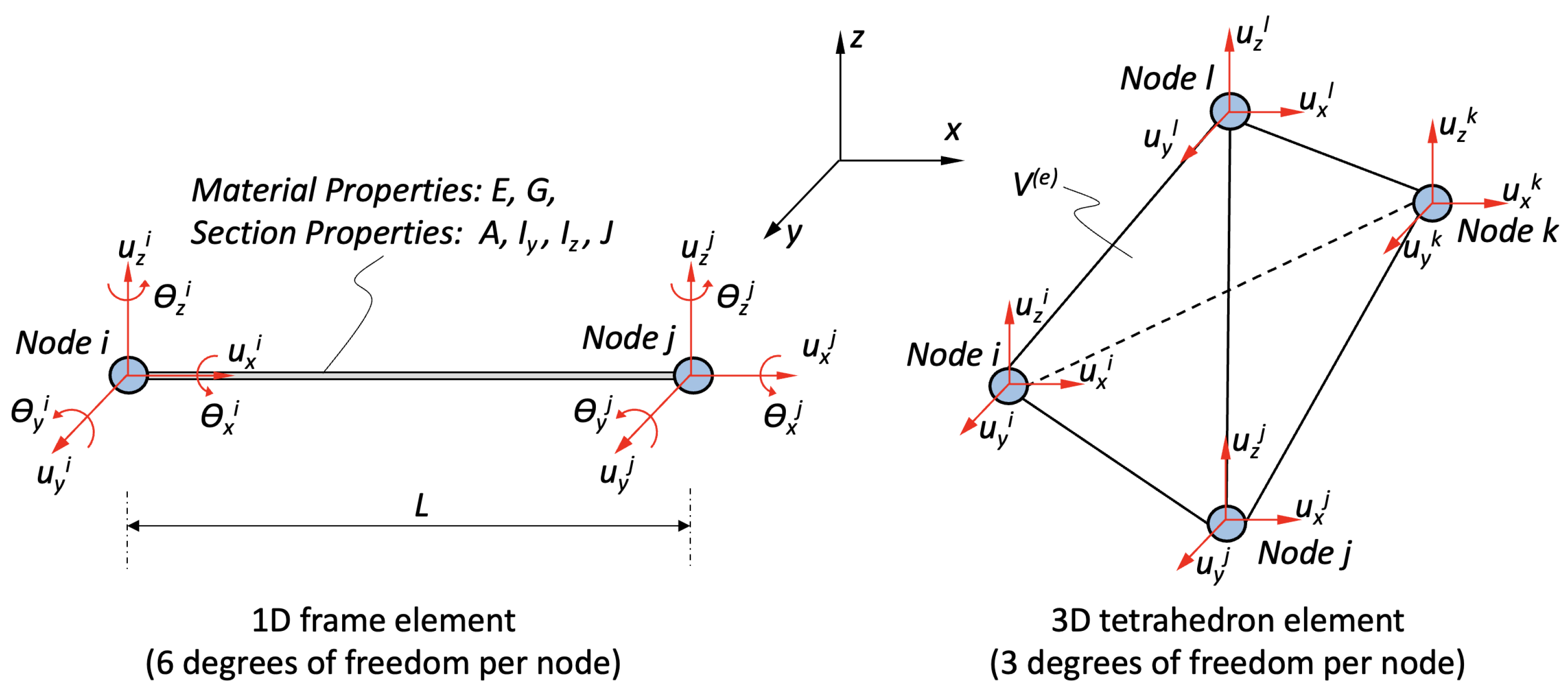
However, for large structures under static and dynamic loads, beam elements (1D elements with 6 degrees of freedom per node) are often used for the analysis [11]. However, in their formulations, these elements cannot account for crack propagation. Therefore, the study of such behavior must adopt more complex models, such as multi-scale methods based on domain decomposition theory [12,13,14,15,16,17,
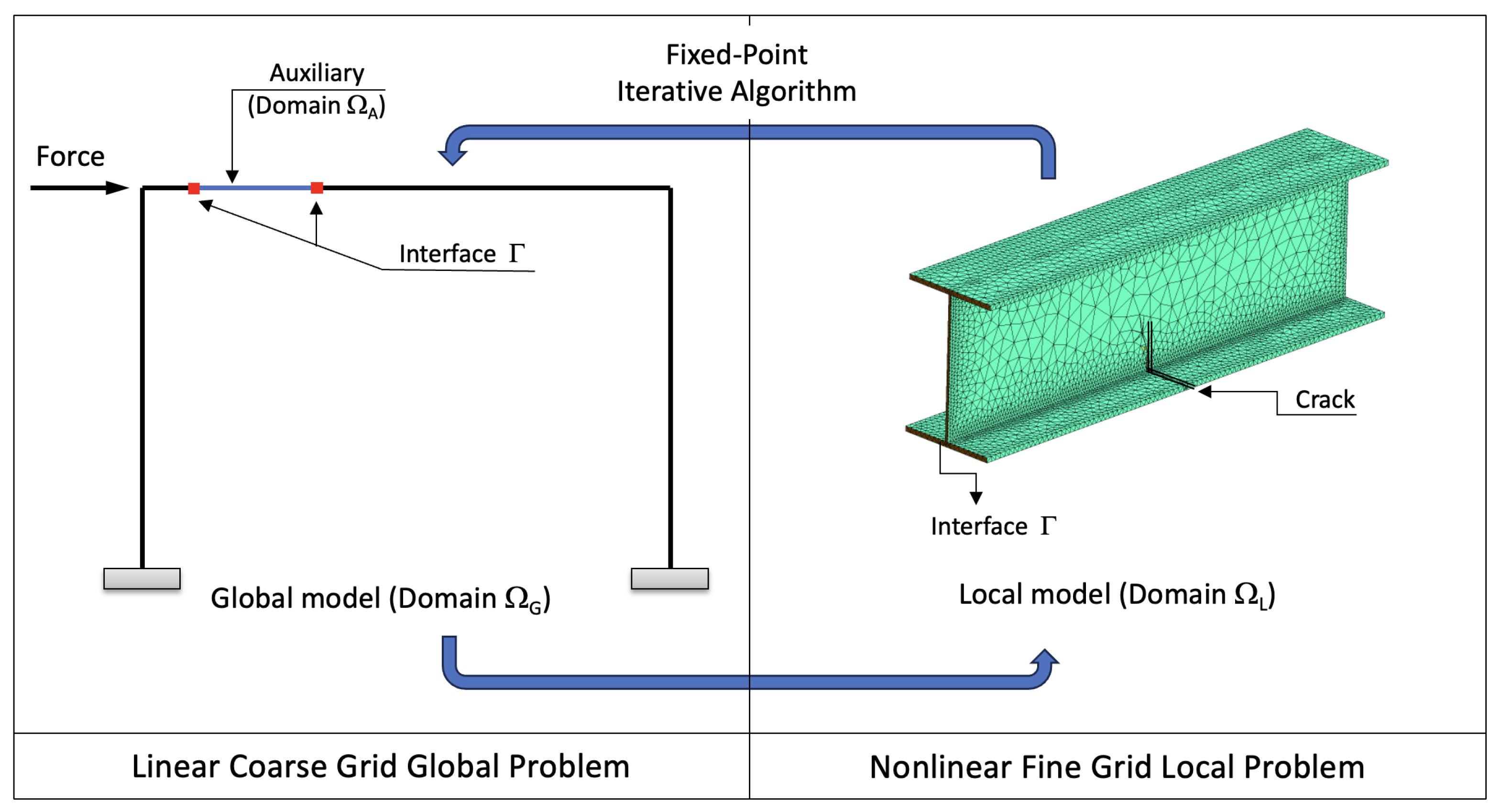
18]. New types of analysis have been studied, involving an iterative solution between local non-linear models coupled with global linear models, called global–local non-intrusive analysis [19].
Global–local non-intrusive analysis uses previously optimized linear and non-linear solvers available in commercial software. These solutions are introduced into the linear model of the structure in the form of displacements and/or forces without the need to modify it [18].
This analysis has been used to estimate crack propagation, non-linear hardening behavior, and non-linear contact, among other complex behaviors, with less computational time compared to a non-decomposed model (also known as a monolithic model) [20,21,22,23,24,25].
The global–local non-intrusive methodology has great advantages, but its convergence depends on the size of the domain of the local model. For example, global–local analysis with mesh refinement was performed in [26,27,28]. A local domain size with a large number of degrees of freedom is preferable since it ensures convergence and results in a better solution; however, it would increase computational costs.
In the implementation of global–local non-intrusive analysis with 1D-to-3D coupling performed in [25], it can be seen that the convergence depends on the length of the local model, which is determined by changing the number of iterations and their errors. Therefore, it is necessary to know the optimal dimensions to ensure the convergence of the methodology.
One way to determine the optimal size of the local model is to use machine learning (ML) techniques. ML is a class of artificial intelligence that seeks to make predictions from available datasets and algorithms [29]. ML techniques have been used to predict the strength of structural elements, for example, the shear strength in beams [30,31,32] and joints [33,34]. Also, they have been used to determine the axial resistance in steel [35,36,37] and concrete elements [38,39,40]. Other ML applications include damage detection [41,42,43,44,45] and structural analysis and design [46,47,48,49], among others.
There are three main stages in the development of an ML model [29]:
  • Prepare the database: The data used to build models are presented in the form of input variables (features) and output variables (labels, categories, or classes). In the case of structures, geometric dimensions and material properties can be classified as features, whereas resistance and deflection are used as labels. In this step, it is important to perform a classification analysis in order to identify the main features among different experiments and to group large amounts of data, considering certain variables that adequately explain certain analyzed behaviors. The features of the initial data and the performance of the learning algorithm affect the accuracy of ML models.
  • Learn: This step aims to train some of the existing ML algorithms using the data obtained from the previous step.
  • Evaluate the model: With the ML model trained, the performance is evaluated using a loss function as a performance indicator.
Some of the ML algorithms used for structural design problems and performance evaluation include linear regression, kernel regression, tree-based algorithms, logistic regression, support vector machines, k-nearest neighbors, discriminant analysis, and artificial neural networks and their variants [50].
Linear and quadratic discriminant analysis [51,52] are appealing because they have closed-form solutions that are easy to compute, are inherently multiclass, and have no hyperparameters to fit, achieving good accuracy. Some applications can be found in [53,54,55].
Therefore, this work applies machine learning techniques in the area of finite-element methods applied to global–local analysis and is organized as follows. The methodology section presents a summary of the global–local non-intrusive methodology, the different cases to be studied, and the mathematical formulation of the categorical discriminant analyses to be used. In the results section, the convergence of the cases is presented, as well as the results of the discriminant analysis. The validation cases using complete structures and the decision function are also introduced, i.e., a functional relationship between the length of the local model and the crack position. Finally, the discussion section summarizes the research and the results obtained, concluding with possible future studies on this topic.

2. Methodology

2.1. Global–Local Non-Intrusive Analysis with 1D-To-3D Coupling

Global–local non-intrusive analysis is performed using SAP2000 software for the linear global problem, with a 1D frame model (with 6 degrees of freedom, or d.o.f., for each node), as presented in Figure 1, and Code_Aster software for the local non-linear solution of the crack propagation, with 3D tetrahedron elements with 3 d.o.f. per node.
Global–local non-intrusive analysis solves a finite-element problem within a fixed-point algorithm by dividing its components into two or more parts: a linear coarse-grid global problem ( Ω G ) and one or more local fine-grid non-linear problems ( Ω L ). The non-linear behavior of this study is limited to crack propagation. The different domains are presented in Figure 2.
The coupling of the models is performed using Code-Aster software, communicating the displacements and forces between the global model and the local non-linear model using the comtypes Python library. The complete methodology for coupling 1D frames with 3D elements is presented in [25]:
  • The equation systems for the global problem are solved using SAP2000, returning the displacements of the global domain u G n + 1 , as presented in Equation (1):
    K G u G n + 1 = f d G + C G T P n
    where K G and f d G are the stiffness matrix and external load vector of the global model Ω G , respectively. The coupling operators that transform quantities in the whole domain into the interfaces C G and P n are the compensation forces related to the fixed-point algorithm used in the global–local non-intrusive method.
  • As the software enables obtaining the nodal reaction forces of an embedded substructure, the auxiliary problem is solved, returning λ A n + 1 in the interface zone. In the case that certain software does not enable obtaining the nodal reaction forces directly, Equation (2) must be used:
    K A u A n + 1 | Γ C A T λ A n + 1 = f d A
    where K A , f d A , and λ A n + 1 are the stiffness matrix, external load vector, and interface reaction forces for the auxiliary domain Ω A , respectively.
    The interface displacements of the auxiliary domain u A n + 1 | Γ can be obtained from the global model displacement, considering the following Equation (3):
    u A n + 1 | Γ = C A u A n + 1 = C G u G n + 1
    where C A is an operator that transforms quantities from the auxiliary domain Ω A into the interface Γ , and C G was previously defined.
  • A non-linear local problem is solved using Code_Aster software, imposing displacements onto the nodes of the interface Γ . After the non-linear problem is solved, i.e., a number of propagation steps are completed, the final displacements of the local model are obtained using Equation (4):
    u L n + 1 | Γ = C L u L n + 1 = P r G L { C G u G n + 1 }
    where C L , u L n + 1 | Γ , and P r G L are the coupling operator, the interface displacements, and the projector operator from the global 1D to the local 3D domain Ω L , respectively.
    The reaction forces λ L n + 1 of the local model in the interface are obtained using Equation (5):
    K L u L n + 1 | Γ C L T λ L n + 1 = f d L
    where K L , f d L , and λ L n + 1 are the stiffness matrix, the external load vector, and the reaction forces at the interface in the domain Ω L .
  • The local reaction forces are then integrated and transformed into three equivalent forces and moments, as per the 6 degrees of freedom used in SAP2000. This is performed using the PROJ_CHAMP operator in Code_Aster.
  • With the local and auxiliary forces calculated, the correction forces for the next iteration P n are obtained using Equation (6):
    P n + 1 = λ A n + 1 + P r L G { λ L n + 1 }
    where the projector operator P r L G , from the local to the global domain, is solved using the aforementioned PROJ_CHAMP operator in Code_Aster.
In order to estimate the best choice of the local model length, a set of three structures is considered to perform global–local non-intrusive analysis, with different lengths and heights for a simple one-bay one-story moment-resisting frame. A total of 39 cases of wide beam sections, length patches, and different locations of the initial crack are considered. A summary of the geometrical configurations for the cases is presented in Figure 3.
The basic properties of the structures are presented in Table 1, Table 2 and Table 3, separated by the length of the original frame beam.
All models presented in Table 1, Table 2 and Table 3 have the same Young’s modulus of 200,000 (MPa), a Poisson ratio ν of 0.3, grade 50 steel (50 ksi or 345 MPa yield stress), a lateral force in the upper node of 100 (kN), and three propagation steps.
As shown in Table 1, Table 2 and Table 3, three sections were analyzed, considering different initial positions of the crack before propagation. The initial geometrical properties of each section are presented in Table 4. The cracked section is depicted in Figure 4 for a wide-flange steel section.
Using the section properties (non-cracked and initially cracked) and different lengths of the cases, the stiffness and ratios between section properties can be calculated to obtain the relation between the properties and the results of the non-intrusive analysis, as well as deriving a discriminant function.

2.2. Machine Learning Models

In order to find the functional relation between the overall results of the non-intrusive analysis and its geometrical properties, a classification or categorical analysis must be performed.
In this section, we discuss some of the most widely employed classification models and present their strengths and limitations. Machine learning is an artificial intelligence discipline with the objective of improving the performance of a specific process using training data based on previous experiences or simulations. The training is carried out by creating mathematical models with adjustable parameters, which are optimized during the learning process. These models can be used to obtain future predictions or extract information from the data, among others [56,57]. It is important to mention that machine learning models achieve the best interpretability and results when simple features and mathematical models are considered [57].

2.2.1. Classification Models

Classification models are mathematical models within a supervised scheme that are designed to approach problems, where a given dataset must be assigned a certain category based on observed features [56,58]. Some of the most commonly used methods are as follows:
  • Linear Discriminant Analysis and Quadratic Discriminant Analysis: These types of discriminant analysis consist of two classifiers with linear and quadratic decision boundaries, respectively. These automatic supervised learning techniques are used for classification and dimensionality reduction. The objective is to find a linear combination of features that maximizes the separation between classes within a dataset. These classification models are attractive due to their closed-form solutions that can be easily calculated. They have been proven to work well with small datasets for training and because there are no hyperparameters to be adjusted [59]. Their advantages are, for example, when the classes are linearly or quadratically separable and the covariances are equal. Interpretability is another strength since the coefficients of the resulting linear combinations provide information on the most relevant characteristics for the separation of the classes. Their disadvantages are, for example, sensitivity to equality of covariances since they assume that the covariances of the classes are equal. Additionally, valid results are only accepted in the domain of training the independent variables [60].
  • Support Vector Machines: Support vector machines are powerful supervised learning algorithms used in both classification and regression tasks. The main objective is to find an optimal separation hyperplane that maximizes the margin between the classes. Their benefits include efficiency in high-dimensional spaces since they can efficiently handle datasets with a large number of attributes, robustness since they have the ability to generalize and are less prone to overfitting, and flexibility in the kernel, allowing the use of different kernel functions such as linear, polynomial, and radial basis functions (RBF), making them adaptable to a wide range of problems and data structures. Their disadvantages include the selection of the appropriate hyperparameters and their inefficiency on large datasets, as they can be computationally expensive and difficult to interpret since they can be less intuitive in terms of parameter interpretation [61].
  • Nearest Neighbors Classification: K-nearest neighbor (K-NN) classification is a supervised machine learning method used to address classification problems. Its main focus is to assign a class label to a data instance based on the class labels of the closest training instances in a feature space. Its benefits include its conceptual simplicity since it is easy to understand and implement; adaptability since it can learn relatively well, including nonlinear and multiclass classification problems; suitability for small datasets; and the nonparametric algorithm used since it does not make assumptions about the functional form of the data. Its disadvantages include that the choice of the number of neighbors (K) is critical and can significantly affect the performance of K-NN, and it is sensitive to scale, so it is important to perform adequate normalization before applying it [62].
  • Decision Tree Classifier: This is a supervised machine learning method whose main objective is to create a tree model that partitions the feature space into decision nodes, where each node represents a region or dataset with a specific class label. The benefits of this model include its interpretability, which allows the model’s decision-making process to be visualized and understood. In addition, it can handle datasets that include both numerical and categorical characteristics. Moreover, it requires little data preparation since it does not require data normalization, it can efficiently handle missing values, and it is effective in detecting interactions since it can capture non-linear relationships and detect interactions between features. The disadvantages include that it tends to overfit the training data if its growth is not adequately controlled. Furthermore, it can exhibit instability since it is sensitive to small variations in the training data, which can result in different trees for similar datasets. Finally, it has limitations in a complex class separation where classes overlap or very complex separation is required and a tendency to be biased toward dominant classes, as it may have difficulty in handling unbalanced datasets [63].
  • Random Forest: This is a decision tree-based machine learning algorithm used for both classification and regression problems. Unlike a single decision tree, random forest creates a collection of trees and combines their predictions for more robust and accurate results. Its benefits include high precision, as it tends to achieve high prediction accuracy on a variety of datasets and problems; robustness against overfitting, as by combining multiple trees, random forest reduces the tendency to overfit; and its ability to effectively handle missing data and outliers, without the need for extensive preprocessing. Its disadvantages include its low interpretability because although each tree within a random forest is interpretable, the combination of many trees can make the model difficult to interpret. Another disadvantage is the need to configure each of the hyperparameters, such as the number of trees and the maximum depth, which must be adjusted appropriately to optimize performance. Finally, the computational efficiency and running time are disadvantages due to the construction of multiple trees and the combination of predictions [64].
Due to the small dataset and the need for a reliable model that is easy to interpret and can generate a closed-form equation of the classification results, in this study, linear and quadratic discriminant analyses are used.

2.2.2. Discriminant Analysis

To perform a discriminant analysis, the following assumptions and restrictions must be considered [65]:
  • One variable is considered categorical and the others are numerical intervals or values, independent of the categorical variables.
  • Two minimum cases are needed in order to generate at least two clusters or groups.
  • The number of discriminant variables must be less than the number of cases minus 2, i.e., x 1 , , x p , where p < ( n 2 ) and n is the number of observations or cases.
  • Any discriminant variable cannot be a linear combination of two or more discriminant variables.
  • The covariance matrices of each group must be approximately equal.
  • All continuous variables must comply with a multivariate normal distribution.
Assuming a dataset with d features or properties, and k category classes, the conditional probability of the variable x given a category k or P ( x | y = k ) is calculated.
Knowing the probability of each analyzed case and its results, predictions can be calculated using Bayes’ Theorem, as shown in Equation (7).
P ( y = k | x ) = P ( x | y = k ) P ( y = k ) P ( x )
The probability of x, given the category y equal to a class k, i.e., P ( x | y = k ) , is calculated using a multivariate Gaussian distribution, with the probability density in Equation (8):
P ( x | y = k ) = 1 ( 2 π ) d / 2 | C o v k | 1 / 2 exp 1 2 ( x μ k ) t C o v k 1 ( x μ k )
where d corresponds to the number of features used for the analysis, and C o v k corresponds to the covariance matrix of the different categories.
Finally, in order to predict the results of the discriminant analysis, the posterior P ( y = k | x ) is calculated, depending on whether the discriminant is one of the following types:
  • Linear discriminant analysis (LDA): In this case, the posterior is calculated using Equation (9):
    log P ( y = k | x ) = 1 2 ( x μ k ) t C o v 1 ( x μ k ) + log P ( y = k ) + C
    where C o v is the covariance matrix for all classes, μ k is the mean of the classes, and C is a constant.
  • Quadratic discriminant analysis (QDA): In this case, the posterior can be calculated as expressed in Equation (10):
    log P ( y = k | x ) = 1 2 log | C o v | 1 2 ( x μ k ) t C o v k 1 ( x μ k ) + log P ( y = k ) + C
    where C o v is the covariance matrix for each class k, μ k is the mean of the classes, and C is a constant.
It is important to mention that LDA presents a linear decision surface due to the assumption of an equal covariance matrix between all classes. In contrast, there is no assumption on the covariance matrix for quadratic discriminant analysis, resulting in a quadratic decision surface for the analysis.
The result to be considered in both linear and quadratic discriminant analysis is the solution that maximizes the score, calculated using the posterior probabilities.
Both discriminant analyses were performed using the built-in functions provided in the scikit learn package in Python [66].

3. Results

From all the cases analyzed using the global–local non-intrusive analysis, considering three propagation steps, a maximum number of iterations of 50, and a convergence tolerance of t o l = 10 5 , the results presented in Table 5 were obtained.
As evident in Table 5, the convergence depended on the patch length, as well as the depth of the crack with respect to the initial height of the section. In addition, two distinct features were identified:
  • The convergence strongly depended on the patch length. According to Saint Venant’s principle, the discontinuity (crack position) must be far from the interface to neglect the non-linear effects at the end of the local model.
  • The convergence status of the method was observed to depend on the length of the overall beam. This is because a very flexible patch in relation to the auxiliary model can negatively affect the convergence of the method.
Is important to mention that in accordance with the governing equations of fracture mechanics for flexure problems, the second moment of area, the area, the length of the element, and the thickness, or in this case, the area, must be considered [67,68]. In this case, the patch length affected the convergence of the method, as explained by Saint Venant’s principle. Another factor to consider is the relation between the length of the patch and the original beam due to the relation of the stiffness of these elements. This affected the convergence when the local model stiffness was considerably larger with respect to the global model in the non-intrusive global–local coupling. Additionally, the stress intensity factors used for crack propagation in Code_Aster depended on the geometry of the crack and the geometrical properties of the cross-section of the element being analyzed [69].
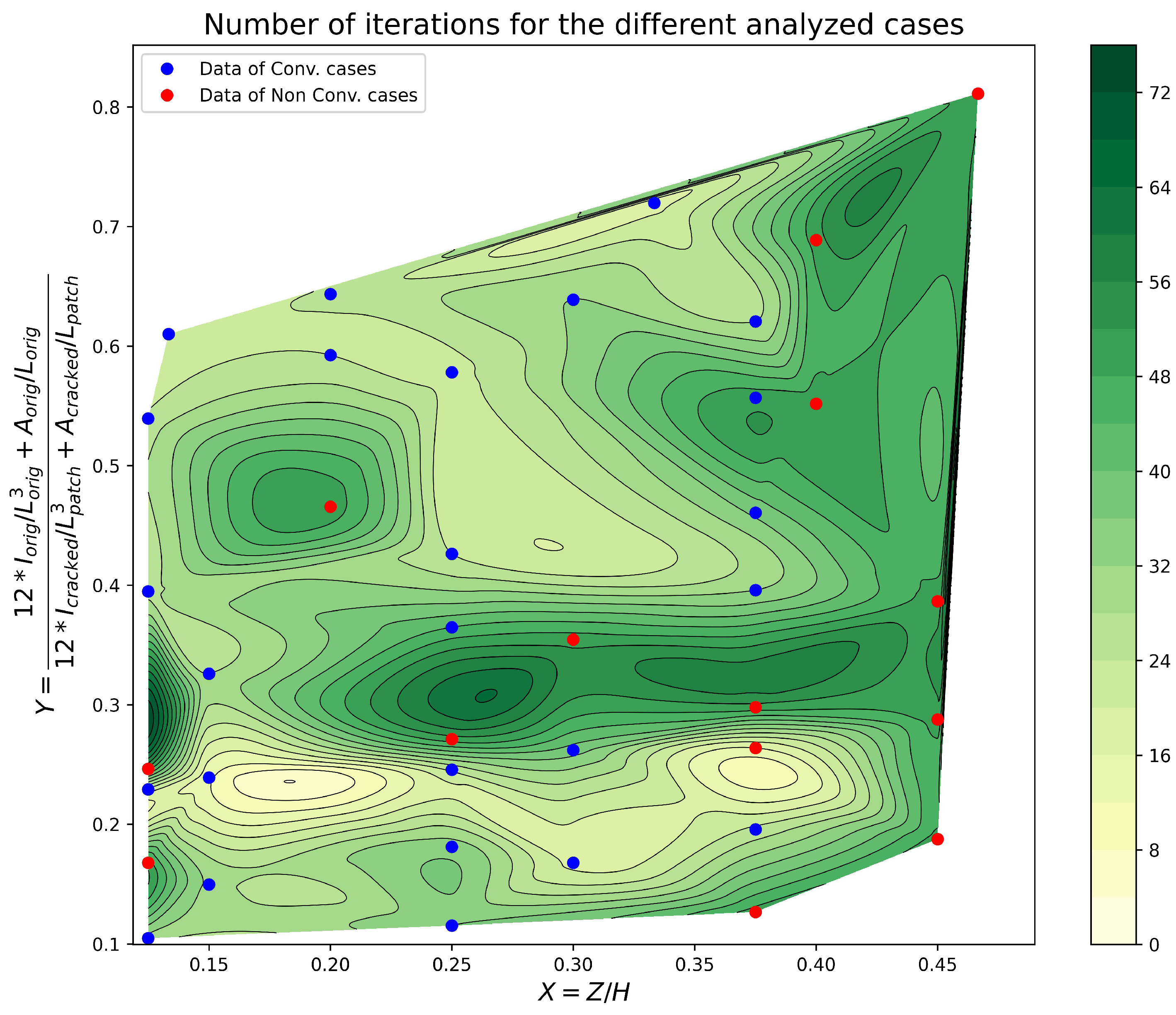
A physics-based analysis of the results indicated that the stiffness of the beam with respect to the original beam and the location of the crack with respect to the original height of the section should be considered. Hence, the variables to analyze from the different cases are presented in Equations (11) and (12).
X = Z / H
where the ratio Z / H is a dimensionless value corresponding to the percentage of the section initially cracked.
Y = 12 · I o r i g m a j o r / L o r i g 3 + A o r i g / L o r i g 12 · I c r a c k e d m a j o r / L p a t c h 3 + A c r a c k e d / L p a t c h
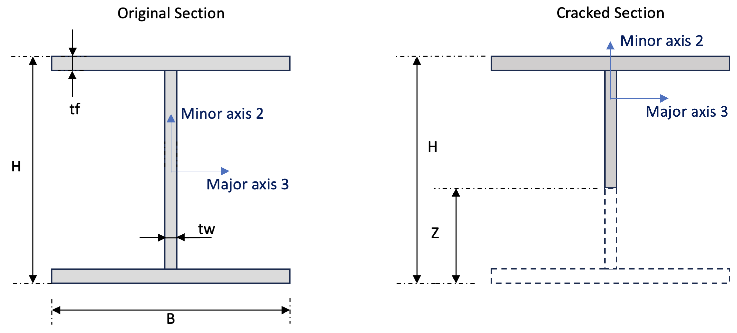
where the numerator in the equation for the dimensionless Y value corresponds to the stiffness contribution of the original non-cracked beam, and the denominator corresponds to the stiffness contribution of the cracked patch, considering only major flexure and axial stresses (based on the original problem). The terms in Equation (12) are the following: I o r i g m a j o r is the non-cracked second-moment area of the cross-section, L o r i g is the complete beam length of the non-cracked beam, A o r i g corresponds to the cross-section area of the non-cracked section, I c r a c k e d m a j o r is the major axis second-moment area of the cracked beam, A c r a c k e d is the cross-section area of the cracked beam, and L p a t c h is the length of the patch used in the analysis.
It is important to highlight that Young’s modulus E in the stiffness contribution in Equation (12) was simplified between the terms of the numerator and the denominator, obtaining the mentioned equation.
The results of the iterations for both features analyzed are presented in Figure 5.
Both discriminant analyses were performed with the analyzed features and the categorical classes, i.e., convergence or non-convergence, and considering that for these cases, no reduction and centering were performed on the data prior to the training of the different discriminant analyses.
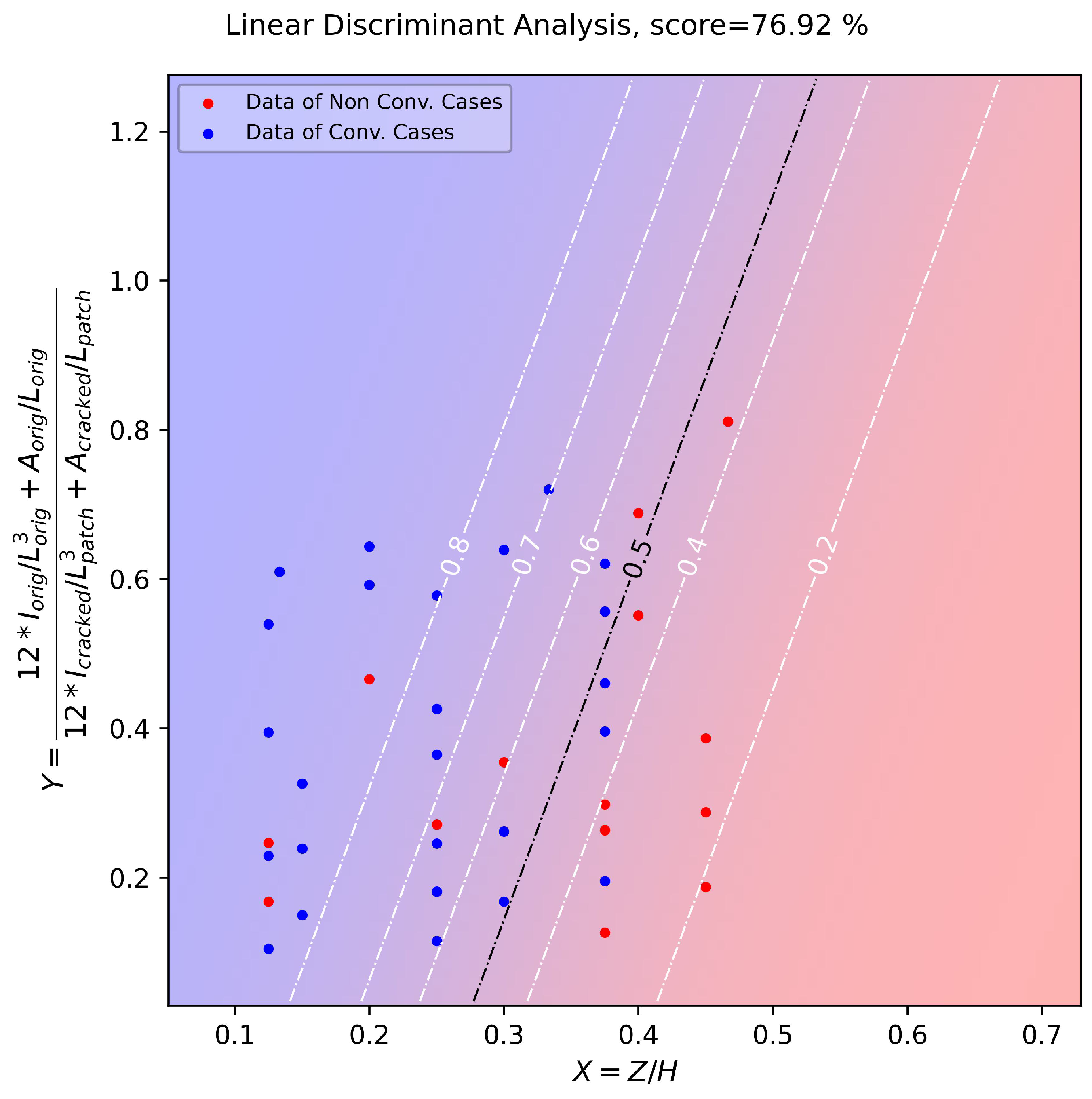
For the linear discriminant analysis presented in Figure 6, the line indicating a 50% probability of convergence is marked in black, representing a score or accuracy of 76.92%, using the features obtained from the data analysis.
Different precision metrics or scores were considered when evaluating the results of the classification performed using linear discriminant analysis, as follows:
  • Micro-Score: This metric is calculated by summing the results of all the classes and calculating the metric over all the datasets. This is the score presented in Figure 6, which is calculated as follows:
    S c o r e M i c r o = T r u e P o s . T r u e P o s . + F a l s e P o s . + F a l s e N e g .
  • Macro-Score: This metric is calculated for each class separately to obtain a simple average of each metric. Each class contributes equally to the calculation of the macro-score, independent of its size.
    S c o r e ( b y c l a s s ) = T r u e P o s . T r u e P o s . + F a l s e P o s . + F a l s e N e g .
    S c o r e M a c r o = S c o r e c l a s s 1 + S c o r e c l a s s 2 2
  • Weighted Score: For this case, the size of each class is considered when calculating the weighted average of each metric. This implies that larger classes have a bigger impact on the final score.
    S c o r e ( b y c l a s s ) = T r u e P o s . T r u e P o s . + F a l s e P o s . + F a l s e N e g .
    S c o r e W e i g h t e d = ( P r o p o r t i o n c l a s s 1 · S c o r e c l a s s 1 ) + ( P r o p o r t i o n c l a s s 2 · S c o r e c l a s s 2 )
The results are as follows:
  • Micro-score: 0.7692
  • Macro-score: 0.7594
  • Weighted score: 0.7647
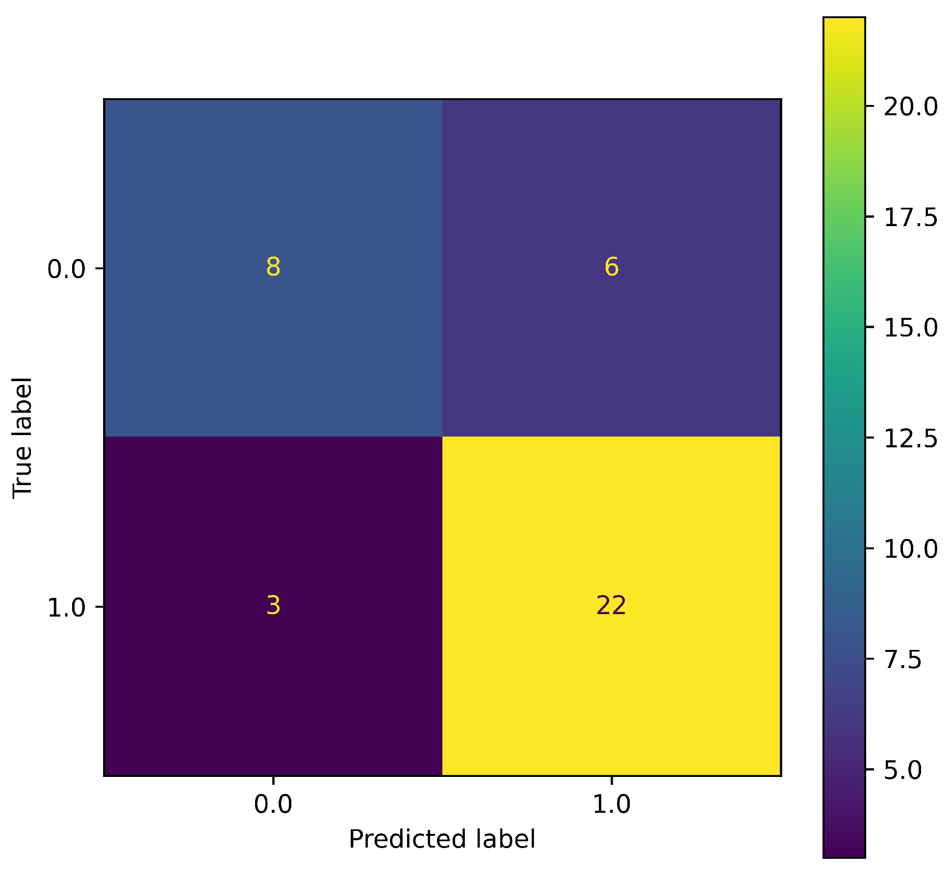
For this case, the weighted metric for the LDA model was considered more relevant due to the consideration of the size of each class when the weighted average was calculated.
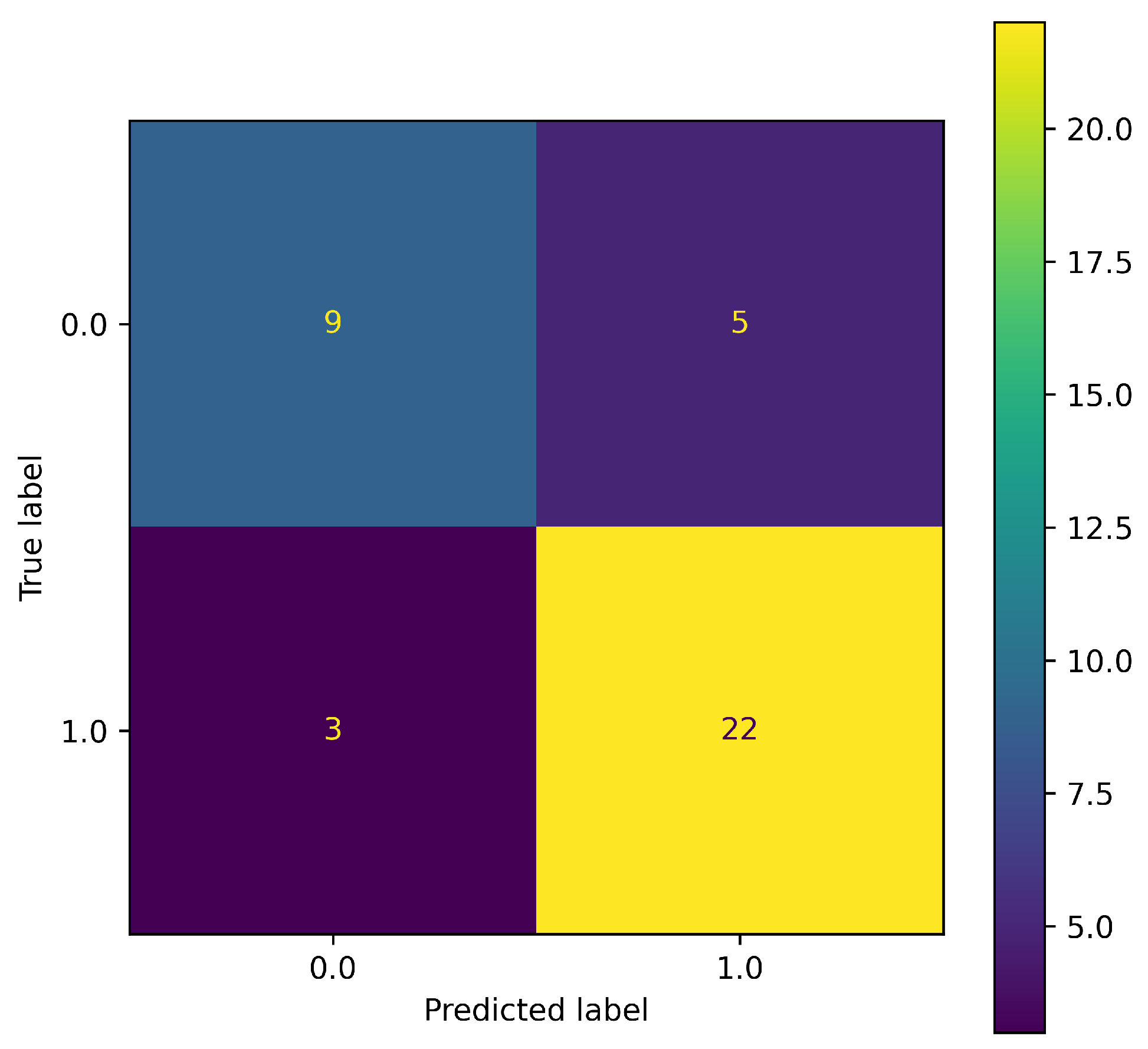
The confusion matrix of the LDA is presented in Figure 7.
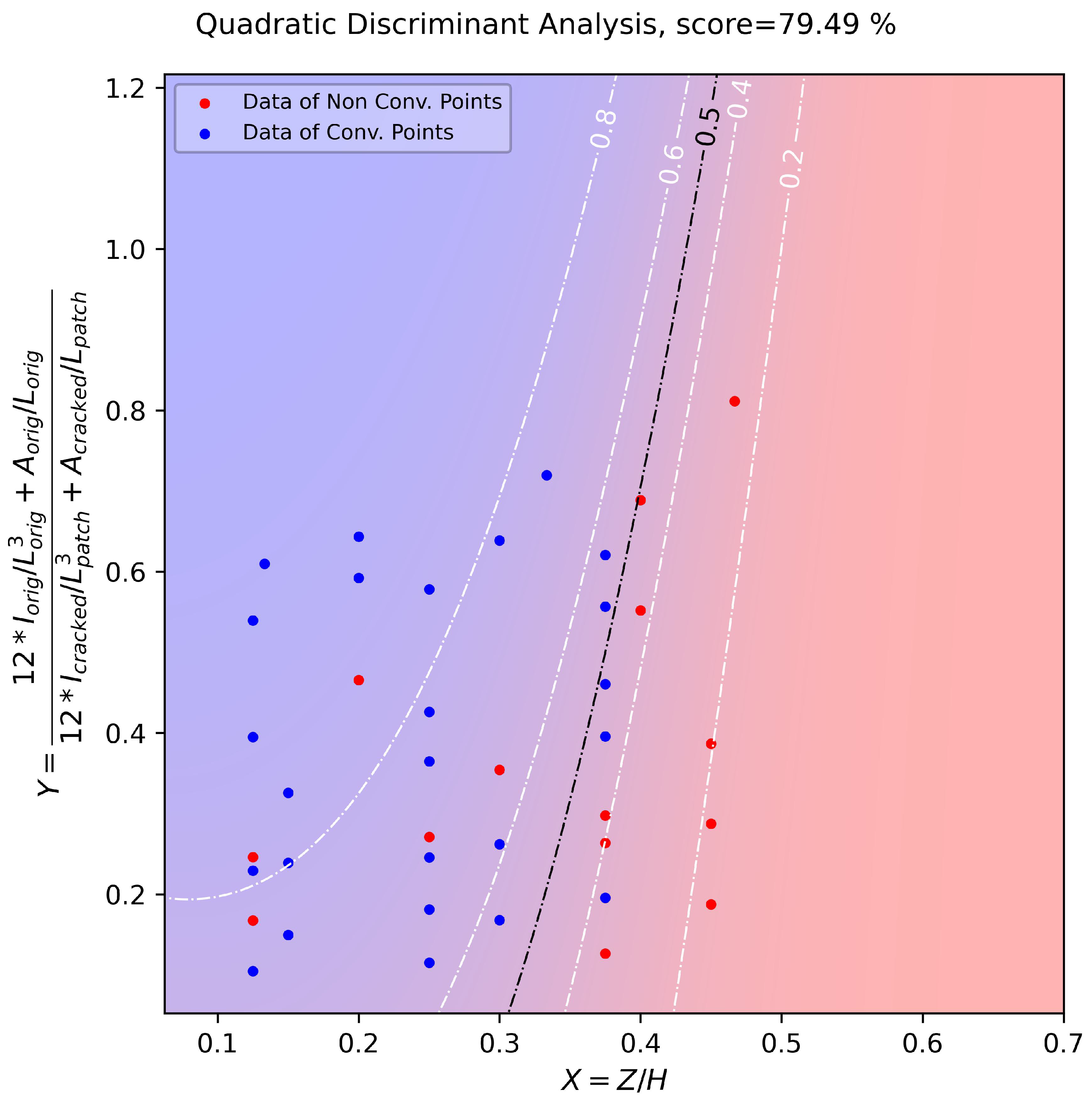
For the QDA presented in Figure 8, the line indicating a 50% probability of convergence is marked in black, representing a score or accuracy of 79.42%, using the features obtained from the data analysis.
For QDA, the same precision metrics presented in Equations (13)–(17) were considered. The results obtained were as follows:
  • Micro-score: 0.7948
  • Macro-score: 0.7824
  • Weighted score: 0.7915
For this case, the weighted metric was considered more relevant due to the consideration of the size of each class when the weighted average was calculated. Finally, the confusion matrix of the QDA is presented in Figure 9.
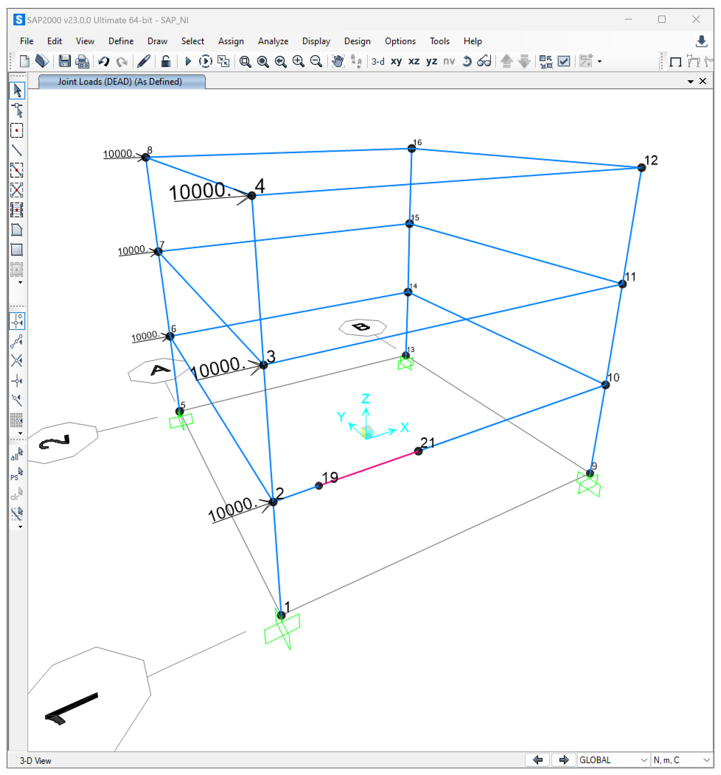
To validate the results of the discriminant analyses, the three-story building presented in [25] with various patches was analyzed with the following properties:
  • A three-story steel structure with a height between floors of 3 m.
  • A span length of 10 m with rigid supports on the column bases.
  • Beam and column sections corresponding to a wide flange, with H = 300 mm, B = 200 mm, tf = 10, and tw = 6 mm.
  • The uncracked inertia in (mm 4 ), uncracked area in (mm 2 ), and complete beam length in (mm) were 95,109,333, 5680, and 10,000 (mm), respectively.
  • The cracked inertia in (mm 4 ) and cracked area in (mm 2 ) were 20,010,062 and 3440, respectively.
  • Four patches were analyzed with local lengths of 1000, 1500, 2000, and 2500 mm.
  • Each local model was analyzed with an initial crack length of 50 mm and three propagation steps.
The SAP2000 model of the software is presented in Figure 10 and was obtained from [25].
The different building cases used for validation are presented in Table 6.
The building cases were incorporated into the discriminant analyses, obtaining different confidence intervals, to ensure the behavior of the global–local analysis.
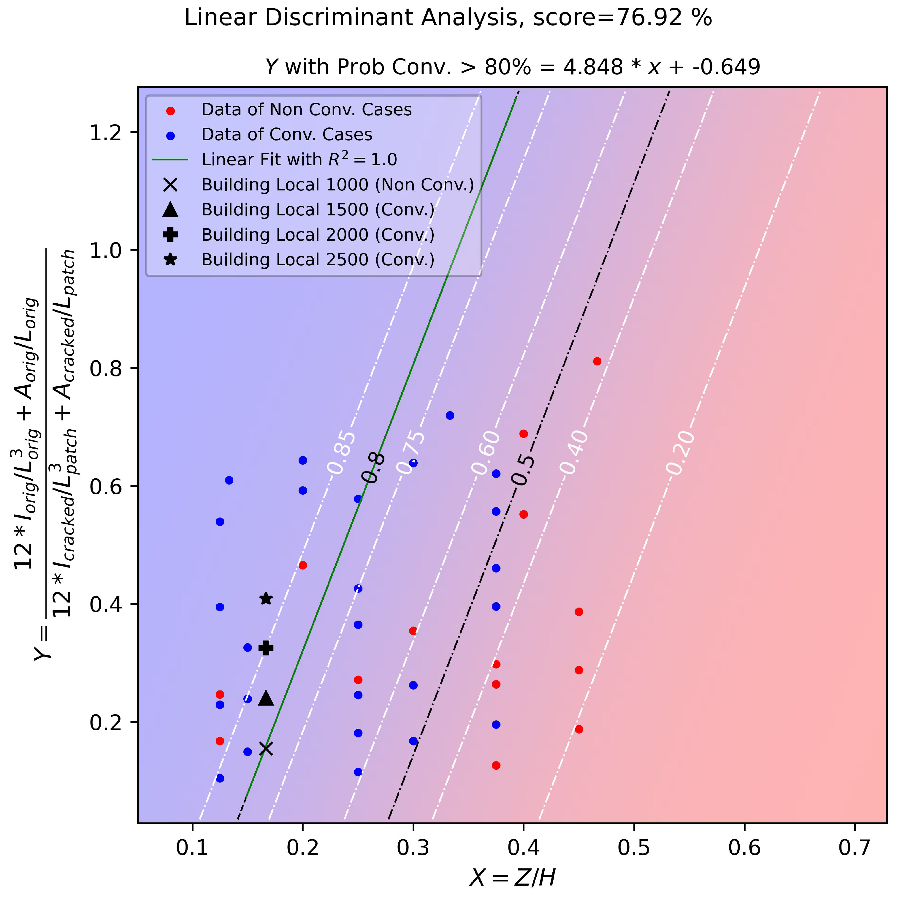
For the linear discriminant analysis, the results are presented in Figure 11.
As presented in Figure 11, to validate the global–local analysis of the building cases, considering a linear discriminant analysis using a contour of the probability of 80%, the convergence for the analyzed cases was achieved using the functional relation from Equation (18) to numerically obtain the patch length:
Y = 12 · I o r i g m a j o r / L o r i g 3 + A o r i g / L o r i g 12 · I c r a c k e d m a j o r / L p a t c h 3 + A c r a c k e d / L p a t c h = 4.848 X 0.649
where X corresponds to the feature Z / H , which relates the initial percentage of the initial crack with respect to the total height of the section. The previous equation is plotted in green in Figure 11, resulting in a linear fit with R 2 = 1.0 .
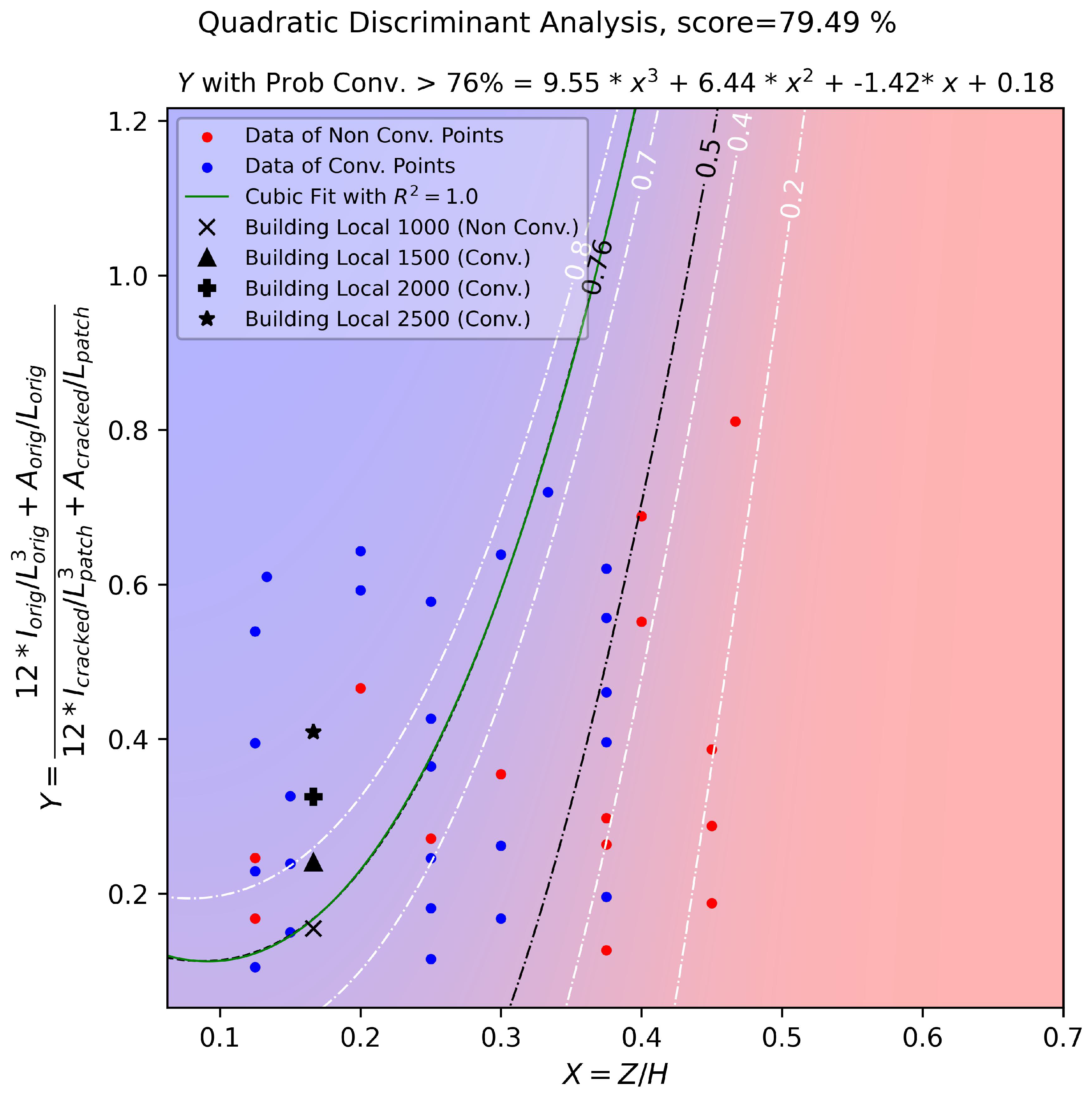
For the quadratic discriminant analysis, the results are presented in Figure 12.
As presented in Figure 12, to validate the quadratic discriminant analysis of the global–local non-intrusive analysis for the building cases, the convergence of the problem was achieved using a contour of the probability of 76%, obtaining the functional relation of Equation (19), and solving for the patch length numerically:
Y = 12 · I o r i g m a j o r / L o r i g 3 + A o r i g / L o r i g 12 · I c r a c k e d m a j o r / L p a t c h 3 + A c r a c k e d / L p a t c h = 9.55 X 3 + 6.44 X 2 1.42 X + 0.18
where X corresponds to the feature Z / H , which relates the initial percentage of the initial crack with respect to the total height of the section. The previous equation is plotted in green in Figure 12, resulting in a cubic polynomial fit with R 2 = 1.0 .
For Equations (18) and (19), R 2 is calculated using the following equation:
R 2 = 1 ( D a t a F i t ) 2 ( D a t a m e a n ( D a t a ) ) 2

3.1. Convergence Analysis of the Building Cases

For the building cases, the converged cases were further analyzed in order to consider the execution times, number of iterations for convergence, number of degrees of freedom for the local patch/model, and distance from the 80% confidence line in the LDA and the 76% confidence line in the QDA, as presented in Table 7.
From the converged cases, it was observed that all differences with respect to the probabilistic discriminant analysis calculation of the Y feature allowed obtaining a ratio of at least 1.5, ensuring the convergence of the building cases. It was also observed that the difference between the local models was negligible relative to the first convergence, i.e., a patch length of 1500 mm, and the iterations. However, for the number of degrees of freedom, there was a difference of +16% and +37% for patch lengths of 2000 and 2500 mm, respectively. Regarding the execution time, there was a difference with respect to the 1500 mm patch of +13% and +16%, and patch lengths of 2000 and 2500 mm, respectively. It can be added that from the discriminant analysis of the building cases, a patch length of 1500 mm was suggested to be used (using the functional relation and a safety factor of 1.5, obtaining a patch length of 1490 mm using the LDA Y feature from Equation (21) and 1555 mm using the QDA Y feature from Equation (22), respectively).
Y ( S . F = 1.5 ) = 12 · I o r i g m a j o r / L o r i g 3 + A o r i g / L o r i g 12 · I c r a c k e d m a j o r / L p a t c h 3 + A c r a c k e d / L p a t c h = 4.848 X 0.649
Y ( S . F = 1.5 ) = 12 · I o r i g m a j o r / L o r i g 3 + A o r i g / L o r i g 12 · I c r a c k e d m a j o r / L p a t c h 3 + A c r a c k e d / L p a t c h = 9.55 X 3 + 6.44 X 2 1.42 X + 0.18
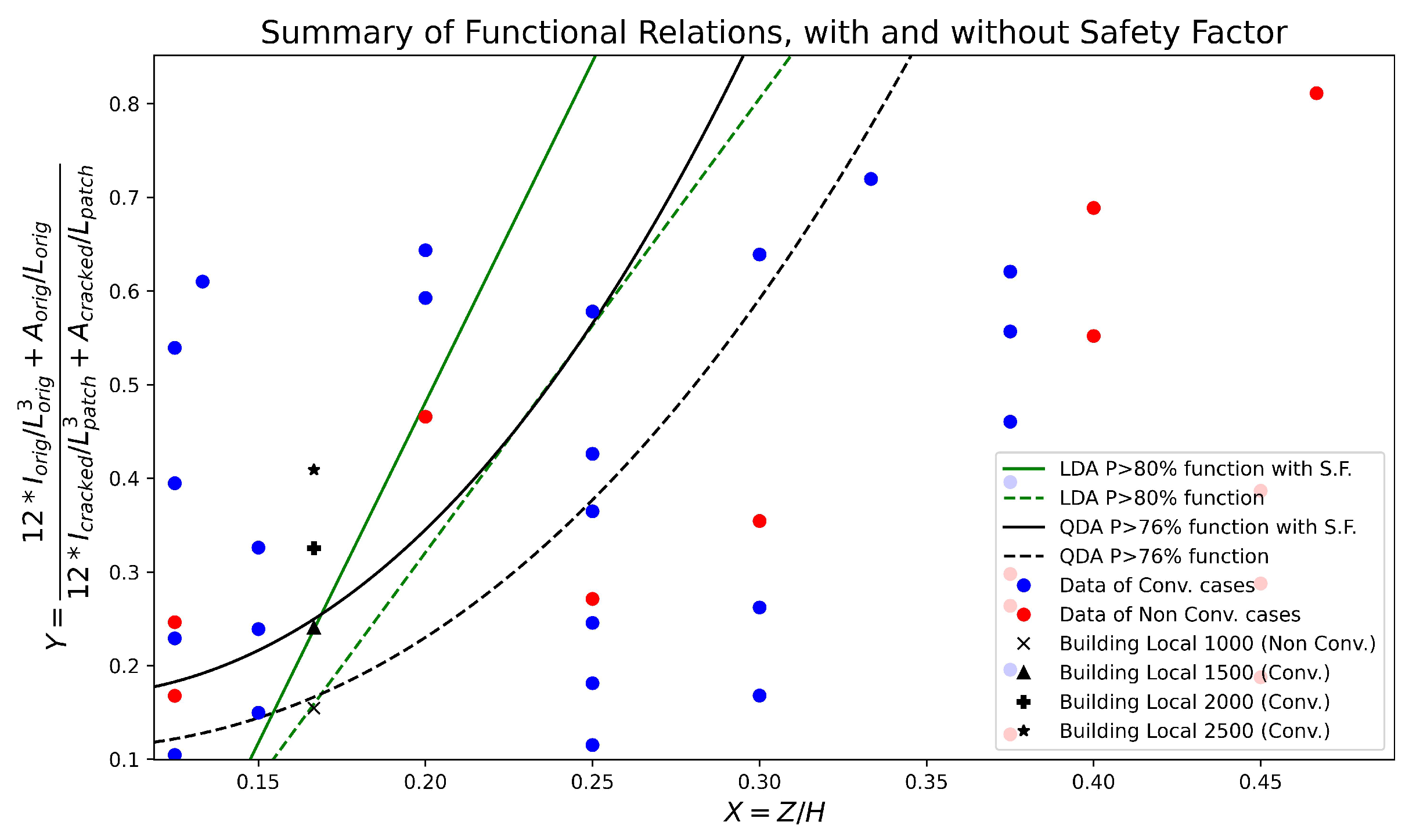
Finally, the equations, both with and without safety factors are presented in Figure 13, summarizing the functional relations obtained in this work.

3.2. Summary of the Results

Performing linear discriminant analysis (LDA) and quadratic discriminant analysis (QDA) within the global–local non-intrusive method enables the training and generation of distinct probabilistic results. The results are presented as contours, facilitating the selection of the optimal patch length and ensuring convergence for doubly symmetric wide-flange elements. This machine learning technique serves as a starting point for solving the problem of defining the optimal patch length. The validation for both discriminant analyses was performed with a three-story building model with varying patch lengths, calculating a safety factor of 1.5 to ensure crack propagation within the local model while minimizing computational resources in the non-intrusive methodology. The presented decision variables take into account the difference in stiffness between the local and global models in the area of interest in order to determine the optimal patch length.

4. Discussion

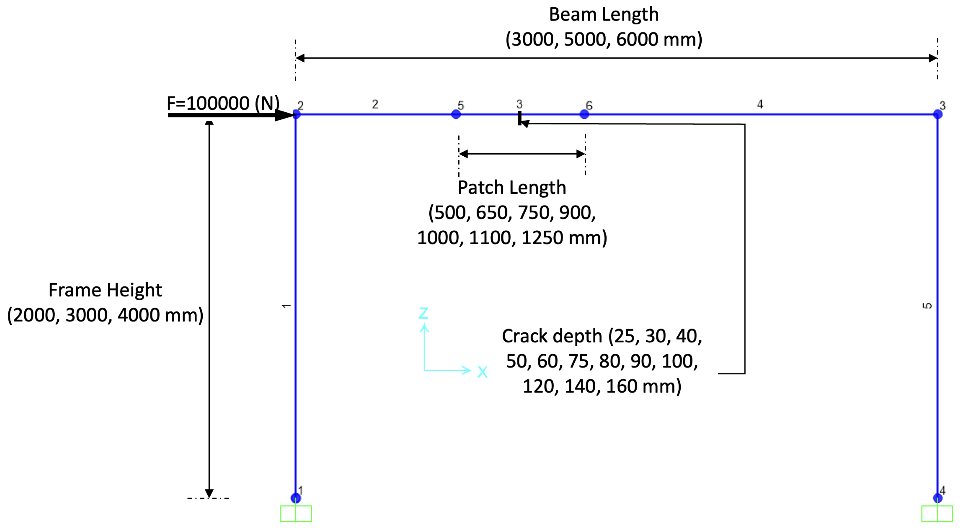
Global–local non-intrusive analysis with 1D-to-3D coupling is a technique that allows us to more efficiently analyze localized discontinuities; however, the length of the local non-linear patch is unknown a priori. Therefore, discriminant analysis was performed using 39 one-bay one-story moment-resisting frames with lateral loads, three propagation steps, and different lengths of the local models or patches.
The categorical analysis was performed using linear and quadratic discriminants, resulting in an accuracy or score greater than 75% in both cases. Nevertheless, the quadratic discriminant analysis performed better, achieving an accuracy of 79%.
Out of the four building cases analyzed, three of them achieved convergence. A 75% confidence contour was considered for QDA, and an 80% confidence level was used for LDA, resulting in a good correlation with the different building models.
From the analysis, a safety factor of 1.5 was recommended to achieve convergence, avoiding excessive degrees of freedom in the local model, i.e., the length of the model was directly related to the number of d.o.f. of the model. This safety factor must be multiplied in the Y feature obtained from the analysis to ensure the expected behavior of the global–local analysis.
The execution time was also taken into account to consider the overall increase in time when larger patches were used relative to the suggested patch with a safety factor of 1.5. The execution time was observed to be 37% greater for the larger local patch compared to the recommended patch from the analysis.
Finally, from the linear and discriminant analyses, a functional relationship between the crack location and the overall height of the section was obtained, allowing for the extrapolation of the ratio between the axial and flexure stiffness of the patch and beam. This allowed us to easily obtain the length of the patch for the local model, ensuring the convergence of the model with a confidence level of 75% or greater.
In future research, more complex machine learning techniques could be used, such as neural networks, support vector machines, and feature selection, among others. More cases are also needed to apply these types of methods, including varying the crack positions, lengths of patches, and types of sections (channels, angles, tubulars, etc.) to be considered in these future analyses.

Author Contributions

Conceptualization, E.C.-I., I.F.-H. and M.J.-Z.; methodology, E.C.-I., I.F.-H. and M.J.-Z.; software, I.F.-H., E.C.-I. and M.J.-Z.; validation, I.F.-H., E.C.-I., M.J.-Z. and J.H.; formal analysis, E.C.-I., M.J.-Z. and J.H.; investigation, I.F.-H., E.C.-I., M.J.-Z. and J.H.; resources, M.J.-Z. and I.F.-H.; data curation, E.C.-I., M.J.-Z. and I.F.-H.; writing—original draft preparation, E.C.-I., M.J.-Z. and I.F.-H.; writing—review and editing, I.F.-H. and J.H.; visualization, E.C.-I., M.J.-Z. and I.F.-H.; supervision, I.F.-H.; project administration, J.H.; funding acquisition, I.F.-H. and J.H. All authors have read and agreed to the published version of the manuscript.

Funding

This work was partly funded by ANID, grant number PFCHA/DOCTORADO BECAS CHILE/2021-21211486 and BECA ESTUDIO DE DOCTORADO, UNIVERSIDAD DE TALCA. The APC was funded by the Faculty of Engineering, Campus Curicó, University of Talca.

Data Availability Statement

The data presented in this study are available in https://doi.org/10.3390/math11112540.

Conflicts of Interest

The authors declare no conflict of interest.

References

  1. ANSI/AISC 360–10; Specification for Structural Steel Buildings. American Institute of Steel Construction: Chicago, IL, USA, 2010.
  2. ANSI/AISC 341–16; Seismic Provision for Structural Steel Buildings. American Institute of Steel Construction: Chicago, IL, USA, 2016.
  3. Juhászová, T.; Miarka, P.; Jindra, D.; Kala, Z.; Seitl, S. Evaluation of Fatigue Crack Growth Rates in an IPE Beam Made of AISI 304 under Various Stress Ratios. Procedia Struct. Integr. 2023, 43, 172–177. [Google Scholar] [CrossRef]
  4. Lou, T.; Wang, W.; Li, J. Seismic behaviour of a self-centring steel connection with replaceable energy-dissipation components. Eng. Struct. 2023, 274, 115204. [Google Scholar] [CrossRef]
  5. Machado, W.G.; da Silva, A.R.; das Neves, F.d.A. Dynamic analysis of composite beam and floors with deformable connection using plate, bar and interface elements. Eng. Struct. 2019, 184, 247–256. [Google Scholar] [CrossRef]
  6. Dexter, R.J.; Connor, R.J.; Mahmoud, H. Review of steel bridges with fracture-critical elements. Transp. Res. Rec. 2005, 1928, 74–82. [Google Scholar] [CrossRef]
  7. Frangopol, D.M.; Soliman, M. Life-cycle of structural systems: Recent achievements and future directions. In Structures and Infrastructure Systems; Routledge: London, UK, 2019; pp. 46–65. [Google Scholar]
  8. Moës, N.; Dolbow, J.; Belytschko, T. A finite element method for crack growth without remeshing. Int. J. Numer. Methods Eng. 1999, 46, 131–150. [Google Scholar] [CrossRef]
  9. Belytschko, T.; Black, T. Elastic crack growth in finite elements with minimal remeshing. Int. J. Numer. Methods Eng. 1999, 45, 601–620. [Google Scholar] [CrossRef]
  10. Khoei, A.R. Extended Finite Element Method: Theory and Applications; John Wiley & Sons: Hoboken, NJ, USA, 2014. [Google Scholar]
  11. Valipour, H.R.; Foster, S.J. Nonlocal Damage Formulation for a Flexibility-Based Frame Element. J. Struct. Eng. 2009, 135, 1213–1221. [Google Scholar] [CrossRef]
  12. Roux, F.X. Method of finite element tearing and interconnecting and its parallel solution algorithm. Int. J. Numer. Methods Eng. 1991, 32, 1205–1227. [Google Scholar]
  13. Whitcomb, J.D. Iterative global/local finite element analysis. Comput. Struct. 1991, 40, 1027–1031. [Google Scholar] [CrossRef]
  14. Pebrel, J.; Rey, C.; Gosselet, P. A Nonlinear Dual-Domain Decomposition Method: Application to Structural Problems with Damage. Int. J. Multiscale Comput. Eng. 2008, 6, 251–262. [Google Scholar] [CrossRef]
  15. Hinojosa, J.; Allix, O.; Guidault, P.A.; Cresta, P. Domain decomposition methods with nonlinear localization for the buckling and post-buckling analyses of large structures. Adv. Eng. Softw. 2014, 70, 13–24. [Google Scholar] [CrossRef]
  16. Guidault, P.A.; Allix, O.; Champaney, L.; Navarro, J.P. A two-scale approach with homogenization for the computation of cracked structures. Comput. Struct. 2007, 85, 1360–1371. [Google Scholar] [CrossRef]
  17. Kerfriden, P.; Allix, O.; Gosselet, P. A three-scale domain decomposition method for the 3D analysis of debonding in laminates. Comput. Mech. 2009, 44, 343–362. [Google Scholar] [CrossRef]
  18. Oumaziz, P.; Gosselet, P.; Boucard, P.A.; Guinard, S. A non-invasive implementation of a mixed domain decomposition method for frictional contact problems. Comput. Mech. 2017, 60, 797–812. [Google Scholar] [CrossRef]
  19. Allix, O.; Gosselet, P. Non intrusive global/local coupling techniques in solid mechanics: An introduction to different coupling strategies and acceleration techniques. In Modeling in Engineering Using Innovative Numerical Methods for Solids and Fluids; Springer: Berlin/Heidelberg, Germany, 2020; pp. 203–220. [Google Scholar]
  20. Duval, M.; Passieux, J.C.; Salaün, M.; Guinard, S. Non-intrusive Coupling: Recent Advances and Scalable Nonlinear Domain Decomposition. Arch. Comput. Methods Eng. 2016, 23, 17–38. [Google Scholar] [CrossRef]
  21. Passieux, J.C.; Réthoré, J.; Gravouil, A.; Baietto, M.C. Local/global non-intrusive crack propagation simulation using a multigrid X-FEM solver. Comput. Mech. 2013, 52, 1381–1393. [Google Scholar] [CrossRef]
  22. Noii, N.; Aldakheel, F.; Wick, T.; Wriggers, P. An adaptive global–local approach for phase-field modeling of anisotropic brittle fracture. Comput. Methods Appl. Mech. Eng. 2020, 361, 112744. [Google Scholar] [CrossRef]
  23. Blanchard, M.; Allix, O.; Gosselet, P.; Desmeure, G. Space/time global/local noninvasive coupling strategy: Application to viscoplastic structures. Finite Elem. Anal. Des. 2019, 156, 1–12. [Google Scholar] [CrossRef]
  24. Fuenzalida-Henriquez, I.; Oumaziz, P.; Castillo-Ibarra, E.; Hinojosa, J. Global-Local non intrusive analysis with robin parameters: Application to plastic hardening behavior and crack propagation in 2D and 3D structures. Comput. Mech. 2022, 69, 965–978. [Google Scholar] [CrossRef]
  25. Jaque-Zurita, M.; Hinojosa, J.; Fuenzalida-Henríquez, I. Global–Local Non Intrusive Analysis with 1D to 3D Coupling: Application to Crack Propagation and Extension to Commercial Software. Mathematics 2023, 11, 2540. [Google Scholar] [CrossRef]
  26. Duarte, C.A.; Kim, D.J. Analysis and applications of a generalized finite element method with global-local enrichment functions. Comput. Methods Appl. Mech. Eng. 2008, 197, 487–504. [Google Scholar] [CrossRef]
  27. Fonseca, G.M.; Barros, F.B.; de Oliveira, T.S.; Monteiro, H.A.; Novelli, L.; Pitangueira, R.L. 2-D Crack propagation analysis using stable generalized finite element method with global-local enrichments. Eng. Anal. Bound. Elem. 2020, 118, 70–83. [Google Scholar] [CrossRef]
  28. Malekan, M.; Barros, F.B. Well-conditioning global–local analysis using stable generalized/extended finite element method for linear elastic fracture mechanics. Comput. Mech. 2016, 58, 819–831. [Google Scholar] [CrossRef]
  29. Thai, H.T. Machine learning for structural engineering: A state-of-the-art review. Structures 2022, 38, 448–491. [Google Scholar]
  30. Abambres, M.; Lantsoght, E.O. Neural network-based formula for shear capacity prediction of one-way slabs under concentrated loads. Eng. Struct. 2020, 211, 110501. [Google Scholar] [CrossRef]
  31. Mohammadhassani, M.; Saleh, A.; Suhatril, M.; Safa, M. Fuzzy modelling approach for shear strength prediction of RC deep beams. Smart Struct. Syst. 2015, 16, 497–519. [Google Scholar] [CrossRef]
  32. Chou, J.S.; Ngo, N.T.; Pham, A.D. Shear strength prediction in reinforced concrete deep beams using nature-inspired metaheuristic support vector regression. J. Comput. Civ. Eng. 2016, 30, 04015002. [Google Scholar] [CrossRef]
  33. Kotsovou, G.M.; Cotsovos, D.M.; Lagaros, N.D. Assessment of RC exterior beam-column Joints based on artificial neural networks and other methods. Eng. Struct. 2017, 144, 1–18. [Google Scholar] [CrossRef]
  34. Sarothi, S.Z.; Ahmed, K.S.; Khan, N.I.; Ahmed, A.; Nehdi, M.L. Predicting bearing capacity of double shear bolted connections using machine learning. Eng. Struct. 2022, 251, 113497. [Google Scholar] [CrossRef]
  35. Sakla, S.S. Neural network modeling of the load-carrying capacity of eccentrically-loaded single-angle struts. J. Constr. Steel Res. 2004, 60, 965–987. [Google Scholar] [CrossRef]
  36. Djerrad, A.; Fan, F.; Zhi, X.D.; Wu, Q.J. Artificial neural networks (ANN) based compressive strength prediction of afrp strengthened steel tube. Int. J. Steel Struct. 2020, 20, 156–174. [Google Scholar] [CrossRef]
  37. Xu, Y.; Zhang, M.; Zheng, B. Design of cold-formed stainless steel circular hollow section columns using machine learning methods. Structures 2021, 33, 2755–2770. [Google Scholar]
  38. Cascardi, A.; Micelli, F.; Aiello, M.A. An Artificial Neural Networks model for the prediction of the compressive strength of FRP-confined concrete circular columns. Eng. Struct. 2017, 140, 199–208. [Google Scholar] [CrossRef]
  39. Raza, A.; Shah, S.A.R.; Ul Haq, F.; Arshad, H.; Raza, S.S.; Farhan, M.; Waseem, M. Prediction of axial load-carrying capacity of GFRP-reinforced concrete columns through artificial neural networks. Structures 2020, 28, 1557–1571. [Google Scholar]
  40. Bakouregui, A.S.; Mohamed, H.M.; Yahia, A.; Benmokrane, B. Explainable extreme gradient boosting tree-based prediction of load-carrying capacity of FRP-RC columns. Eng. Struct. 2021, 245, 112836. [Google Scholar] [CrossRef]
  41. Tran-Ngoc, H.; Khatir, S.; De Roeck, G.; Bui-Tien, T.; Wahab, M.A. An efficient artificial neural network for damage detection in bridges and beam-like structures by improving training parameters using cuckoo search algorithm. Eng. Struct. 2019, 199, 109637. [Google Scholar] [CrossRef]
  42. Hasni, H.; Alavi, A.H.; Jiao, P.; Lajnef, N. Detection of fatigue cracking in steel bridge girders: A support vector machine approach. Arch. Civ. Mech. Eng. 2017, 17, 609–622. [Google Scholar] [CrossRef]
  43. Huang, H.; Burton, H.V. Classification of in-plane failure modes for reinforced concrete frames with infills using machine learning. J. Build. Eng. 2019, 25, 100767. [Google Scholar] [CrossRef]
  44. Lei, Y.; Zhang, Y.; Mi, J.; Liu, W.; Liu, L. Detecting structural damage under unknown seismic excitation by deep convolutional neural network with wavelet-based transmissibility data. Struct. Health Monit. 2021, 20, 1583–1596. [Google Scholar] [CrossRef]
  45. Naderpour, H.; Mirrashid, M. Classification of failure modes in ductile and non-ductile concrete joints. Eng. Fail. Anal. 2019, 103, 361–375. [Google Scholar] [CrossRef]
  46. Hadi, M.N. Neural networks applications in concrete structures. Comput. Struct. 2003, 81, 373–381. [Google Scholar] [CrossRef]
  47. Tashakori, A.; Adeli, H. Optimum design of cold-formed steel space structures using neural dynamics model. J. Constr. Steel Res. 2002, 58, 1545–1566. [Google Scholar] [CrossRef]
  48. Horton, T.A.; Hajirasouliha, I.; Davison, B.; Ozdemir, Z. Accurate prediction of cyclic hysteresis behaviour of RBS connections using deep learning neural networks. Eng. Struct. 2021, 247, 113156. [Google Scholar] [CrossRef]
  49. Truong, V.H.; Vu, Q.V.; Thai, H.T.; Ha, M.H. A robust method for safety evaluation of steel trusses using Gradient Tree Boosting algorithm. Adv. Eng. Softw. 2020, 147, 102825. [Google Scholar] [CrossRef]
  50. Sun, H.; Burton, H.V.; Huang, H. Machine learning applications for building structural design and performance assessment: State-of-the-art review. J. Build. Eng. 2021, 33, 101816. [Google Scholar] [CrossRef]
  51. Murphy, K.P. Machine Learning: A Probabilistic Perspective; MIT Press: Cambridge, MA, USA, 2012. [Google Scholar]
  52. Ghojogh, B.; Crowley, M. Linear and quadratic discriminant analysis: Tutorial. arXiv 2019, arXiv:1906.02590. [Google Scholar]
  53. Khan, A.; Kim, H.S. Classification and prediction of multidamages in smart composite laminates using discriminant analysis. Mech. Adv. Mater. Struct. 2022, 29, 230–240. [Google Scholar] [CrossRef]
  54. Janeliukstis, R.; Rucevskis, S.; Chate, A. Classification-based damage localization in composite plate using strain field data. J. Phys. 2018, 1106, 012022. [Google Scholar] [CrossRef]
  55. Yu, J. Machinery fault diagnosis using joint global and local/nonlocal discriminant analysis with selective ensemble learning. J. Sound Vib. 2016, 382, 340–356. [Google Scholar] [CrossRef]
  56. Angra, S.; Ahuja, S. Machine learning and its applications: A review. In Proceedings of the 2017 International Conference on Big Data Analytics and Computational Intelligence (ICBDAC), Chirala, India, 23–25 March 2017; pp. 57–60. [Google Scholar] [CrossRef]
  57. Castillo-Ibarra, E.; Alsina, M.A.; Astudillo, C.A.; Fuenzalida-Henríquez, I. PFA-Nipals: An Unsupervised Principal Feature Selection Based on Nonlinear Estimation by Iterative Partial Least Squares. Mathematics 2023, 11, 4154. [Google Scholar] [CrossRef]
  58. James, G.; Witten, D.; Hastie, T.; Tibshirani, R. Classification. In An Introduction to Statistical Learning: With Applications in R; Springer: New York, NY, USA, 2021; pp. 129–195. [Google Scholar] [CrossRef]
  59. Ledoit, O.; Wolf, M. Honey, I Shrunk the Sample Covariance Matrix. SSRN Electron. J. 2003. [Google Scholar] [CrossRef]
  60. Jombart, T.; Devillard, S.; Balloux, F. Discriminant analysis of principal components: A new method for the analysis of genetically structured populations. BMC Genet. 2010, 11, 94. [Google Scholar] [CrossRef]
  61. Cortes, C.; Vapnik, V. Support-vector networks. Mach. Learn. 1995, 20, 273–297. [Google Scholar] [CrossRef]
  62. Cover, T.; Hart, P. Nearest neighbor pattern classification. IEEE Trans. Inf. Theory 1967, 13, 21–27. [Google Scholar] [CrossRef]
  63. Alpaydin, E. Introduction to Machine Learning, 2nd ed.; The MIT Press: Cambridge, MA, USA, 2010. [Google Scholar]
  64. Breiman, L. Random forests. Mach. Learn. 2001, 45, 5–32. [Google Scholar] [CrossRef]
  65. Hastie, T.; Tibshirani, R.; Friedman, J. Linear Methods for Classification. In The Elements of Statistical Learning: Data Mining, Inference, and Prediction; Springer: New York, NY, USA, 2009; pp. 101–137. [Google Scholar] [CrossRef]
  66. Pedregosa, F.; Varoquaux, G.; Gramfort, A.; Michel, V.; Thirion, B.; Grisel, O.; Blondel, M.; Prettenhofer, P.; Weiss, R.; Dubourg, V.; et al. Scikit-learn: Machine Learning in Python. J. Mach. Learn. Res. 2011, 12, 2825–2830. [Google Scholar]
  67. Tada, H.; Paris, P.C.; Irwin, G.R. The Stress Analysis of Cracks Handbook, 3rd ed.; ASME Press: New York, NY, USA, 2000. [Google Scholar] [CrossRef]
  68. Anderson, T.L. FRACTURE MECHANICS: Fundamentals and Applications, 4th ed.; CRC Press: Boca Raton, FL, USA, 2017. [Google Scholar] [CrossRef]
  69. EDF. Code Aster/Salome-Meca Module 2: Advanced Training; EDF: Paris, France, 2017. [Google Scholar]
Figure 1. Degrees of freedom per node for 1D frame elements (using SAP2000) and 3D tetrahedron elements (using Code_Aster).
Symmetry 15 02068 g001
Figure 2. Reference mechanical problem (domain of the Ω R structure).
Symmetry 15 02068 g002
Figure 3. Summary of the geometrical configurations for all cases.
Symmetry 15 02068 g003
Figure 4. Original and cracked section of a wide-flange steel section.
Symmetry 15 02068 g004
Figure 5. Contour lines for the number of iterations for all 39 cases analyzed.
Symmetry 15 02068 g005
Figure 6. Linear discriminant analysis for the 39 cases.
Symmetry 15 02068 g006
Figure 7. Confusion matrix of LDA.
Symmetry 15 02068 g007
Figure 8. Quadratic discriminant analysis for the 39 cases.
Symmetry 15 02068 g008
Figure 9. Confusion matrix of QDA.
Symmetry 15 02068 g009
Figure 10. SAP2000 3-story building.
Symmetry 15 02068 g010
Figure 11. Linear discriminant analysis with building cases.
Symmetry 15 02068 g011
Figure 12. Quadratic discriminant analysis with building cases.
Symmetry 15 02068 g012
Figure 13. Linear and quadratic discriminant analyses with building cases and safety factors.
Symmetry 15 02068 g013
Table 1. Analyzed models using the global–local non-intrusive method for a length of 3000 mm and height of 2000 mm.
CaseSection * (H × B × tf × tw in mm)Original Depth of Crack (mm)Beam Patch Length (mm)Complete Beam Length L orig (mm)Uncracked Area A orig (mm 2 )Uncracked Inertia I orig (mm 4 )
1H200 × 200 × 8 × 6255003000430432,623,018
2H200 × 200 × 8 × 6505003000430432,623,018
3H200 × 200 × 8 × 6755003000430432,623,018
4H200 × 200 × 8 × 6506503000430432,623,018
5H200 × 200 × 8 × 6756503000430432,623,018
6H200 × 200 × 8 × 6257503000430432,623,018
7H200 × 200 × 8 × 6507503000430432,623,018
8H200 × 200 × 8 × 6757503000430432,623,018
9H200 × 200 × 8 × 6759003000430432,623,018
10H200 × 200 × 8 × 62510003000430432,623,018
11H200 × 200 × 8 × 65010003000430432,623,018
12H200 × 200 × 8 × 67510003000430432,623,018
13H300 × 150 × 8 × 64012503000410462,624,352
14H300 × 150 × 8 × 66012503000410462,624,352
15H300 × 150 × 8 × 610012503000410462,624,352
16H300 × 150 × 8 × 614012503000410462,624,352
17H400 × 300 × 16 × 1080900300013,280395,629,227
18H400 × 300 × 16 × 10160900300013,280395,629,227
19H400 × 300 × 16 × 10801100300013,280395,629,227
20H400 × 300 × 16 × 101201100300013,280395,629,227
21H400 × 300 × 16 × 101601100300013,280395,629,227
* H is the total height of the wide-flange section; B is the total width of the section; tf is the thickness of the flange; and tw is the thickness of the web.
Table 2. Analyzed models using the global-local non-intrusive method for a length of 5000 mm and height of 3000 mm.
CaseSection * (H × B × tf × tw in mm)Original Crack Depth (mm)Beam Patch Length (mm)Complete Beam Length L orig (mm)Uncracked Area A orig (mm 2 )Uncracked Inertia I orig (mm 4 )
22H200 × 200 × 8 × 6305005000430432,623,018
23H200 × 200 × 8 × 6605005000430432,623,018
24H200 × 200 × 8 × 6905005000430432,623,018
25H200 × 200 × 8 × 6307505000430432,623,018
26H200 × 200 × 8 × 6607505000430432,623,018
27H200 × 200 × 8 × 6907505000430432,623,018
28H200 × 200 × 8 × 63010005000430432,623,018
29H200 × 200 × 8 × 66010005000430432,623,018
30H200 × 200 × 8 × 69010005000430432,623,018
* H is the total height of the wide-flange section; B is the total width of the section; tf is the thickness of the flange; and tw is the thickness of the web.
Table 3. Analyzed models using the global-local non-intrusive method for a length of 7000 mm and height of 4000 mm.
CaseSection * (H × B × tf × tw in mm)Original Crack Depth (mm)Beam Patch Length (mm)Complete Beam Length L orig (mm)Uncracked Area A orig (mm 2 )Uncracked Inertia I orig (mm 4 )
31H200 × 200 × 8 × 6255007000430432,623,018
32H200 × 200 × 8 × 6505007000430432,623,018
33H200 × 200 × 8 × 6755007000430432,623,018
34H200 × 200 × 8 × 6257507000430432,623,018
35H200 × 200 × 8 × 6507507000430432,623,018
36H200 × 200 × 8 × 6757507000430432,623,018
37H200 × 200 × 8 × 62510007000430432,623,018
38H200 × 200 × 8 × 65010007000430432,623,018
39H200 × 200 × 8 × 67510007000430432,623,018
* H is the total height of the wide-flange section; B is the total width of the section; tf is the thickness of the flange; and tw is the thickness of the web.
Table 4. Different sections and initial geometrical properties.
Section CaseSection * (H × B × tf × tw in mm)Original Crack Depth (mm)Area of Cracked Section mm 2 Cracked Inertia in Minor Axis mm 4 Cracked Inertia in Major Axis mm 4
S1H200 × 200 × 8 × 62526025,336,3397,054,597
S2H200 × 200 × 8 × 63025725,336,2496,503,006
S3H200 × 200 × 8 × 65024525,335,8894,567,420
S4H200 × 200 × 8 × 66023925,335,7093,754,370
S5H200 × 200 × 8 × 67523025,335,4392,715,291
S6H200 × 200 × 8 × 69022125,335,1691,878,233
S7H300 × 150 × 8 × 64027122,254,53619,314,453
S8H300 × 150 × 8 × 66025922,254,17615,529,984
S9H300 × 150 × 8 × 610023522,253,4569,422,895
S10H300 × 150 × 8 × 614021122,252,7365,078,668
S11H400 × 300 × 16 × 1080784036,025,33371,161,800
S11H400 × 300 × 16 × 10120744036,022,00048,818,746
S11H400 × 300 × 16 × 10160704036,018,66731,461,314
* H is the total height of the wide-flange section; B is the total width of the section; tf is the thickness of the flange; and tw is the thickness of the web.
Table 5. Results of the non-intrusive analysis.
CaseSectionCrack DepthPatch Length (mm)Categorical LabelStatusIterations Until Convergence
1H200255000Non Conv.50
2H200505000Non Conv.50
3H200755000Non Conv.50
4H200506501Conv.44
5H200756501Conv.32
6H200257501Conv.27
7H200507501Conv.24
8H200757501Conv.37
9H200759001Conv.49
10H2002510001Conv.25
11H2005010001Conv.23
12H2007510001Conv.28
13H3004012501Conv.20
14H3006012501Conv.25
15H30010012501Conv.18
16H30014012500Non Conv.50
17H400809000Non Conv.50
18H4001609000Non Conv.50
19H4008011001Conv.24
20H40012011001Conv.32
21H40016011000Non Conv.50
22H200305001Conv.31
23H200605001Conv.19
24H200905000Non Conv.50
25H200307501Conv.13
26H200607501Conv.38
27H200907500Non Conv.50
28H2003010001Conv.28
29H2006010000Non Conv.50
30H2009010000Non Conv.50
31H200255001Conv.30
32H200505001Conv.36
33H200755000Non Conv.50
34H200257500Non Conv.50
35H200507501Conv34
36H200757501Conv25
37H2002510001Conv.23
38H2005010001Conv.25
39H2007510000Non Conv.16
Table 6. Sections and patches used for validation using the 3-story building.
Building Section CaseSectionX Feature (Dimensionless)Y Feature (Dimensionless)Local Patch Length (mm)Status
BS1H300 × 200 × 10 × 60.166670.1546528911000Non-Conv.
BS2H300 × 200 × 10 × 60.166670.240704621500Conv.
BS3H300 × 200 × 10 × 60.166670.3252208022000Conv.
BS4H300 × 200 × 10 × 60.166670.4090516842500Conv.
Table 7. Iterations for convergence, degrees of freedom, and overall execution times for all converged building cases with X = Z / H = 0.1667 ; LDA: Y = 0.1591 ; and QDA: Y = 0.1664 .
Building Section CaseIter. for Conv.Degrees of FreedomExecution Times (s)Y FeatureRatio Y / Y LDA 80 % Ratio Y / Y QDA 76 %
BS1301590.15460.970.92
BS219477033910.24071.511.44
BS320554344420.32522.041.95
BS418657814550.40912.572.45
Disclaimer/Publisher’s Note: The statements, opinions and data contained in all publications are solely those of the individual author(s) and contributor(s) and not of MDPI and/or the editor(s). MDPI and/or the editor(s) disclaim responsibility for any injury to people or property resulting from any ideas, methods, instructions or products referred to in the content.

