An Efficient Trajectory Planning Approach for Autonomous Ground Vehicles Using Improved Artificial Potential Field

Abstract

In this paper, the concept of symmetry is utilized in the promising trajectory planning design of autonomous ground vehicles—that is, the construction and the solution of improved artificial potential field-based trajectory planning approach are symmetrical. Despite existing artificial potential fields (APF) achievements on trajectory planning in autonomous ground vehicles (AGV), applying the traditional approach to dynamic traffic scenarios is inappropriate without considering vehicle dynamics environment and road regulations. This paper introduces a highly efficient approach for planning trajectories using improved artificial potential fields (IAPF) to handle dynamic road participants and address the issue of local minima in artificial potential fields. To begin with, potential fields are created with data obtained from other sensors. By incorporating rotational factors, the potential field will spin when the obstacle executes a maneuver; then, a safety distance model is also developed to limit the range of influence in order to minimize the computational burden. Furthermore, during the planning process, virtual forces using the gradient descent method are generated to direct the vehicle’s movement. During each timestep, the vehicle will assess whether it is likely to encounter a local minimum in the future. Once a local minimum is discovered, the method will create multiple temporary objectives to guide the vehicle toward the global minimum. Consequently, a trajectory that is both collision-free and feasible is planned. Traffic scenarios are carried out to validate the effectiveness of the proposed approach. The simulation results demonstrate that the improved artificial potential field approach is capable of generating a secure trajectory with both comfort and stability.

1. Introduction

Motion planning, as a crucial part of autonomous driving systems (ADS), has received a good deal of interest from the academic community [1,2]. Specifically, creating a safe route free of collisions is the main goal. Despite extensive research on obstacle avoidance algorithms in autonomous ground vehicles (AGV), it is inappropriate to apply these algorithms to traffic scenarios without taking into account vehicle dynamics and road regulations. In order to better suit the traffic environment, the conventional algorithm should be modified to cope with the actual driving scenarios.

Many strategies for addressing trajectory planning have been studied over time by researchers: graph search [3,4], random sampling [5,6], artificial potential field (APF) [7,8,9], numerical optimization [10,11], and AI-based techniques [12]. For example, the two-way A-star method is used in [3] to increase the planning algorithm’s computational efficiency. In order to solve the problem that the traditional A-star algorithm has many inflection points and a long path, the study [4] proposed an improved A-star algorithm that increases the number of search directions. In [6], a novel approach using the Dijkstra optimization-based rapidly exploring random tree algorithm (APSD-RRT) is suggested; it has customizable probability and sample area, and experiments are carried out to show that the proposed approach can achieve significantly better performance in terms of balancing the computation cost and performance compared to original RRT. The work [11] developed a unified path planning system based on the model predictive controller (MPC) that selects the maneuvers’ mode automatically instead of utilizing explicit rules; it implemented a system of limitations in MPC that mandates avoiding collisions between the ego car and neighboring vehicles to guarantee safety. The study [12] solved local-minimum-point issues by combining reinforcement learning with an enhanced black-hole potential field; the method learned how to jump out of local-minimum-point instantly without any prior knowledge.

Even though the efforts mentioned before have been successful, most of them operate assuming that an autonomous vehicle drives in fixed driving circumstances and avoids static obstacles. Rather than finding a feasible path from the starting point to the destination under mostly static conditions, trajectory planning modules of ADSs are actually required to be able to handle a variety of driving situations caused by traffic laws, obstacles, and other road users in a dynamically changing environment. This means that the planner needs to take obstacle motion into account in order to actively handle both static and dynamic traffic obstacles for a range of on-road driving scenarios. Compared to other planning methods that have been proposed, the APF method offers advantages in managing a dynamic environment with low computational costs, even with complex PFs for obstacles and road constructions.

Some studies have been carried out in this field [13,14,15,16,17,18,19,20,21,22]. In [13], a controller-based approach for path planning and tracking collision avoidance is suggested, and the safety distance is added to the APF by creating a safe route in a traffic simulation. The work [15] offered an improved APF method that uses the conventional A* method for time computation while addressing the issue of local minima. The study [18] developed a motion planning strategy that combines an APF-based fuzzy system with a parameter scheduler for auto-mated car collision avoidance systems. In [17] aims to address the limitations of the local minimum and the unsolvable issue of the conventional APF approach; the method is able to quantify the robot’s tendency to become trapped in the mechanical equilibrium condition in APF by detecting variations in the distance between the robot and the target over a specific time period. In [20], an algorithm for energy-efficient local path planning is proposed; they make it possible for AGV to anticipate obstacles by incorporating future movement prediction into the APF method. An enhanced APF approach in [22] is presented to achieve higher accuracy and efficiency by merging the fuzzy control idea to boost stability and adding an angle function to fit with the original force field function.

Despite the success of APF-based techniques, there remain several crucial issues that require solutions. Traditional APF methods, originally designed for addressing trajectory planning issues in mobile robots, exhibit slow response times and tend to produce unachievable trajectories in the presence of steering objects. In addition, APF-based techniques generally prefer to change lanes rather than follow the car, making them inappropriate for on-road driving scenarios. During the planning phase, the host vehicle in the potential field (PF) algorithm is often considered more as a particle rather than an automobile. In order to ensure the safety and practicality of APF-based path planning and collision avoidance methods for ADSs, it is imperative to address these issues.

Hence, to address the local minimum problem and enable the APF method with the ability to follow the obstacle vehicle, this study introduces a novel, improved artificial potential field-based trajectory planning method for real-time planning of autonomous ground vehicles in dynamic environments. The primary contribution of this study is outlined below: An efficient trajectory planning approach using improved APF for AGV is proposed. The APF is able to handle different kinds of obstacles, including static, deaccelerating, and moving at constant speed. By incorporating the future prediction and temporary goal mechanism, the vehicle is able to predict whether the vehicle will enter a local minimum point in advance. Then, the temporary goal will guide the vehicle toward the right lane to avoid any infeasible trajectory. Particularly, we proposed a new way to consider the velocity in the APF method; by combining vehicle velocity, the vehicle is able to perform car-following and move more like a human-driven car. Compared to the traditional APF approach method, the proposed method can plan a smoother, more feasible and collision-free trajectory while adding acceptable computation cost.

The remainder of this article is as follows: Section 2 illustrates the construction of all kinds of potential fields (PFs) for the environment model. The planning method using PFs is described in Section 3. Simulation results are given in Section 4. Section 5 offers a conclusion.

2. Environment Model

2.1. Driving Behavior Analysis

In an on-road driving scenario, the typical driving intentions include cruising, following cars, and changing lanes. In the case of the car following, generally, the host vehicle chooses the following strategy because the host vehicle and the obstacle vehicle are in the same lane. At the same time, the obstacle vehicle shares a similar speed with the host vehicle. If the obstacle vehicle is faster than the host vehicle, this case will become free cruising. If the obstacle vehicle has a much lower speed than the host vehicle, the host will have to perform lane-changing maneuvers to drive faster on the road. For lane-changing cases, the host vehicle is performing lane changing because the other lane is the goal lane of the host vehicle or the lane that the vehicle is driving on is not available due to obstacles or other road participants. As a result, the vehicle needs to change the lane.

The foundation of the APF planning method is the idea that elements of the driving environment, such as goals, road boundaries, and obstacles, can create a potential field similar to an electric field. As Figure 1 shows, under the influence of the force generated by the field, the agent in the field represents the host vehicle as it moves toward the global minimum point. Here, the virtual potential field force is selected to be the negative gradient of the field’s current position, which mathematically indicates the direction of the fastest decline and helps guide the vehicle toward the goal position.

In this paper, the possibility of a collision is naturally lower in this situation. The vehicle, which is frequently thought of as a particle, moves in the field at each time step based on the strength and direction of the force. The trajectory is created by adding the agent positions at each timestep until the agent reaches the target point or the time horizon. Specifically, the x and y coordinates at each time step are combined to be the trajectory.

$$Tra{j}_{APF}=\{{(x,y)}_{t_1}+{(x,y)}_{t_2}+\mathrm{\dots }+{(x,y)}_{t_{n-1}}+{(x,y)}_{t_n}\}$$

(1)

As per the analysis above, the traditional APF method has several problems that need to be improved to accommodate the on-road driving scenario. Firstly, the APF method-based planner only tries to avoid collision by lane change. Due to the APF planning mechanism, the vehicle can only cruise on the road by the effect of road repulsion or change the lane by the effect of obstacle repulsion and goal attraction. This problem is mainly because the traditional APF planning method does not take the velocity changing into consideration. As [13] assumes, the vehicle is driving along the road at a constant speed. Secondly, when the vehicle encounters the local minimum point, the vehicle will be trapped in the local minimum. As Figure 2 shows, the local minimum here is defined as a point where the negative gradient at this point is oriented to a place that might cause a collision. As mentioned above, the planning process of the APF method is definitive. The method needs a mechanism to get rid of the local minimum. Otherwise, the vehicle will be trapped into the local minimum every time.

An improved APF planning method (IAPF) is proposed in this paper to solve the problems. Specifically, the velocity update mechanism is introduced to enable the car to accelerate and decelerate to follow the obstacle car or overtake.

After introducing the velocity update mechanism, the trajectory is:

$$Tra{j}_{IAPF}=\{{(x,y,v,\phi )}_{t_1},{(x,y,v,\phi )}_{t_2},\mathrm{\dots },{(x,y,v,\phi )}_{t_{n-1}},{(x,y,v,\phi )}_{t_n}\}$$

(2)

Then, future prediction and temporary goal mechanisms are designed to solve the local minimum problem. The future prediction will detect the potential local minimum point in advance. Whenever a local minimum is detected, the algorithm creates a temporary goal that generates an attractive force to drag the vehicle to the global minimum.

2.2. Environment Model

In the APF Method, the perception results of sensors are utilized to establish the artificial potential field. The potential field is later concatenated to describe the environment and guide the following planning process. Here, the potential field functions (PFs) are composed of three parts: road boundary repulsion field, goal attraction field, and obstacle repulsion field. The total potential function is defined as the sum of all PFs:

$$U_{Total}=U_{road}+U_{goal}+U_{obtacle}$$

(3)

2.2.1. Road Boundary Repulsion Field

As Figure 2 shows, the standard one-way road is comprised of a road base on each side, a solid line, a broken line, and the road surface between these lines. To strictly follow the traffic rules, the vehicle should never drive out of the solid line, cross the broken line when necessary, and tend to stay at the center of the current lane.

A standard road structure is shown in Figure 2; D_s is the safety distance, and d_w is the width of the lane. Y is the vertical coordinate of the host vehicle; X is the horizontal coordinate of the host vehicle.

Considering the rules above, the road boundary repulsion field is modeled to make the vehicle follow the traffic rules. The road potential can be divided into two parts: boundary potential and center potential:

$$U_{Road}=U_{Bound}+U_{Center}$$

(4)

where U_road stands for the total road potential field value, which is a field concatenated by U_Bound and U_Center. U_Bound is the road boundary field that prevents the car from driving out of the road boundary. U_Center is the description of the broken line function as pushing the vehicle back to the center of the road while small enough not to obstruct the lane change. The expression of U_road is:

$$U_{Road}=\left\{\begin{array}{l}\frac{k_1{d}_w{}^4}{1},Y>d_w\\ k_1(Y-\frac{d_w}{2}){}^4,d_w>Y>\frac{d_w}{2}\\ k_2\cdot (\frac{d_w}{2}-Y{)}^2,Y<\frac{d_w}{2}\end{array}\right.$$

(5)

The field’s amplitude is indicated by the coefficients k₁ and k₂. When the field is appropriately set, as in Figure 3a, it will rise quickly when a vehicle tries to cross a road boundary and pushes back toward the center of the lane without obstructing the vehicle’s ability to change lanes.

As Figure 3a shows, the road boundary field is the combination of U_Bound and U_Center, and the PF value increases rapidly when reaching the road boundary. The U_Center plays the role of maintaining the vehicle in the center of each lane.

2.2.2. Goal Attraction Field

The attraction field is designed to guide the vehicle to travel to the target point or cruise along the road at a certain speed. Here, for different purposes, two kinds of attraction fields are designed to achieve a certain goal.

$$U_{att}=U_{normal}+U_{goal}$$

(6)

where U_normal is used to keep the vehicle driving along the road and U_goal to lead the vehicle to the desired place. During the path planning process, the goal position should be obtained in each planning period by decision module. When goal information is missing, the U_normal will normally lead the vehicle driving along the road. In order to guide the host vehicle, the goal position is described through the following function.

The U_normal is to keep the vehicle driving along the road and cruising at a certain speed v_c. As a result, the expression is:

$$U_{normal}=b_{1}X$$

(7)

The goal attraction field is designed to guide the vehicle toward the goal point. At the same time, to generate a smooth path in the following step, the U_goal is defined as:

$$U_{goal}=b_{2}X-\frac{d_w}{\pi }{b}_3\cos (\frac{\pi }{d_w}(Y-Y_{goal}))$$

(8)

where b₁, b₂, and b₃ are the coefficient of attraction field. X and Y are the horizontal and vertical coordinate values. Y_goal is the vertical coordinate value of the goal position. It is worth noting that in common driving situations on the road, there is no specific goal point that needs to stop in the middle of the road. Figure 3b shows that the goal attraction field linearly decreases in the X direction. In the Y direction, the vehicle near the broken line the field decreasing faster. As a result, the vehicle is able to cross the broken line smoothly.

2.2.3. Obstacle Potential Field

The influence range of the obstacle field is mainly introduced to reduce the computational burden of obstacles far away from the host vehicle. The distance should be reasonably long to ensure the safety of the path, as shown in Figure 4. The influence range based on safety barking distance is shown below:

$$D_S=\frac{v_c{}^2-v_o{}^2}{2a_b}+S_m$$

(9)

where D_S, D_B, and S_m are safety distance, braking distance and safety margin, respectively. V_c and v_o are the velocities of the host and obstacle vehicle. A_b is the maximum braking acceleration of the host vehicle. S_m is a constant number, ensuring extra safety in case of any other accidents.

Specifically, when the algorithm is running in a complex scenario with multiple obstacles, it will compare the distance between the obstacles and the host vehicle; if the distance is larger than the safety distance, the obstacle will be determined to be a safe obstacle for the host. Later in the potential field calculation process, the potential field value of the obstacle will be assigned to 0. As a result, the calculation burden will decrease while maintaining the safety of the algorithm.

The obstacle potential field is responsible for the planning of a collision-free path. In the driving practice, the obstacles have different motion states: some obstacles are static, but others are other road participants who are also driving along the road. Sometimes, these obstacles will also perform lane change maneuvers. The key component of the obstacle potential field is illustrated in the following content of this part.

The obstacle vehicle’s motion state is dynamically changing in response to varying driving intentions. In order to create a more informative potential field that can produce a better trajectory, the risk of an obstacle vehicle with different sizes and headings should be reflected in the potential field’s size and orientation.

A set of weight factors, namely rotation coefficients, are introduced to make the potential field rotate when the obstacle changes its orientation. The field of obstacle potential is expressed as follows:

$$\left\{\begin{array}{l}{R}_X=x\cos \phi -y\sin \phi \\ R_Y=x\sin \phi +y\cos \phi \end{array}\right.$$

(10)

$$U_{obs}=\left\{\begin{array}{l}\cos (\arctan \left(\frac{y-y_o}{x-x_o}\right))*e^{A_x{R}_x{}^2+A_y{R}_y{}^2},\sqrt{{(x-x_o)}^2+{(y-y_o)}^2}<D_s\\ 0,\sqrt{{(x-x_o)}^2+{(y-y_o)}^2}<D_s\end{array}\right.$$

(11)

Here, U_obs is the field of the obstacle vehicle. Φ is the yaw of an obstacle vehicle. A_x and A_y are the size coefficients according to different obstacle sizes.

As Figure 4 shows, Figure 4a,b are the obstacle potential fields of different vehicles that have different sizes and masses. The larger car will have a higher PF value in the center to indicate the potential crash damage. The smaller one will have a lower PF but be able to move agilely. As a result, the overall PF in farther distances is higher than in large-size obstacles.

When the heading angle of the obstacle vehicle is not equal to zero, the potential field will rotate toward the direction of the heading of the obstacle vehicle. Compared to traditional APF, it will depict the movement of the obstacle more accurately.

The potential function of traditional APF used in Figure 5 can be presented as:

$$U_{Otrad}=\frac{1}{2}k\frac{1}{\sqrt{{(x-x_o)}^2+{(y-y_o)}^2}}$$

(12)

As shown in Figure 5, different obstacle potential fields of improved APF and APF approach show how the rotation factor affects the environment model. By incorporating the rotation factor, the potential field will rotate at the same angle as the vehicle heading angle. As a result, the potential field will be more informative while the obstacle vehicle takes the lane change maneuver. The host vehicle will be able to decelerate in advance to generate a more comfortable trajectory.

Figure 5b shows the zigzag trajectory planned by the traditional APF approach, which makes it difficult for the actual controller to follow the result. At the same time, the vehicle in the traditional APF can only move at a constant speed. This fact prevents the traditional APF from decelerating to follow an obstacle car with a speed similar to the host vehicle.

From Figure 4 and Figure 5, it is clear that the potential field of the obstacle is symmetrical. The design of the potential field function in the form of symmetry accords with the natural symmetry in the driving environment. When the potential field function is designed in a symmetrical form, the symmetrical potential field will naturally help the planning of lane change behavior without judging the specific direction of the lane change maneuver. Furthermore, when the rotation factor is combined, the symmetrical potential field enables the potential field of obstructed vehicles in all directions to have a logical influence on the movement of the main vehicle.

3. Trajectory Generation

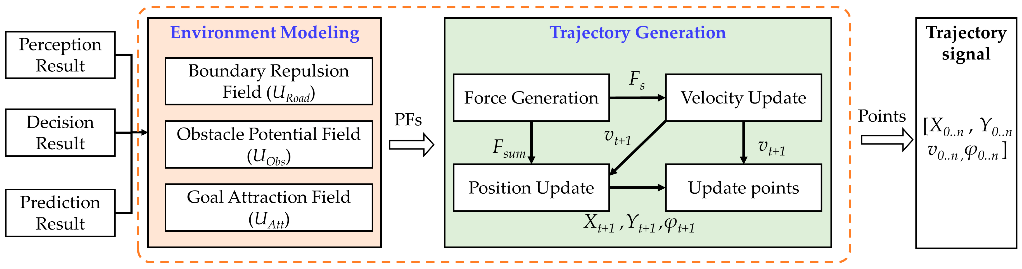
In this section, the potential fields are used to plan the collision-free, smooth and feasible trajectory. In contrast to the traditional APF method, the velocity is introduced into the planning process to plan the trajectory. The planning process is made up of three parts: virtual force generation, local minimum detection, and movement calculation.

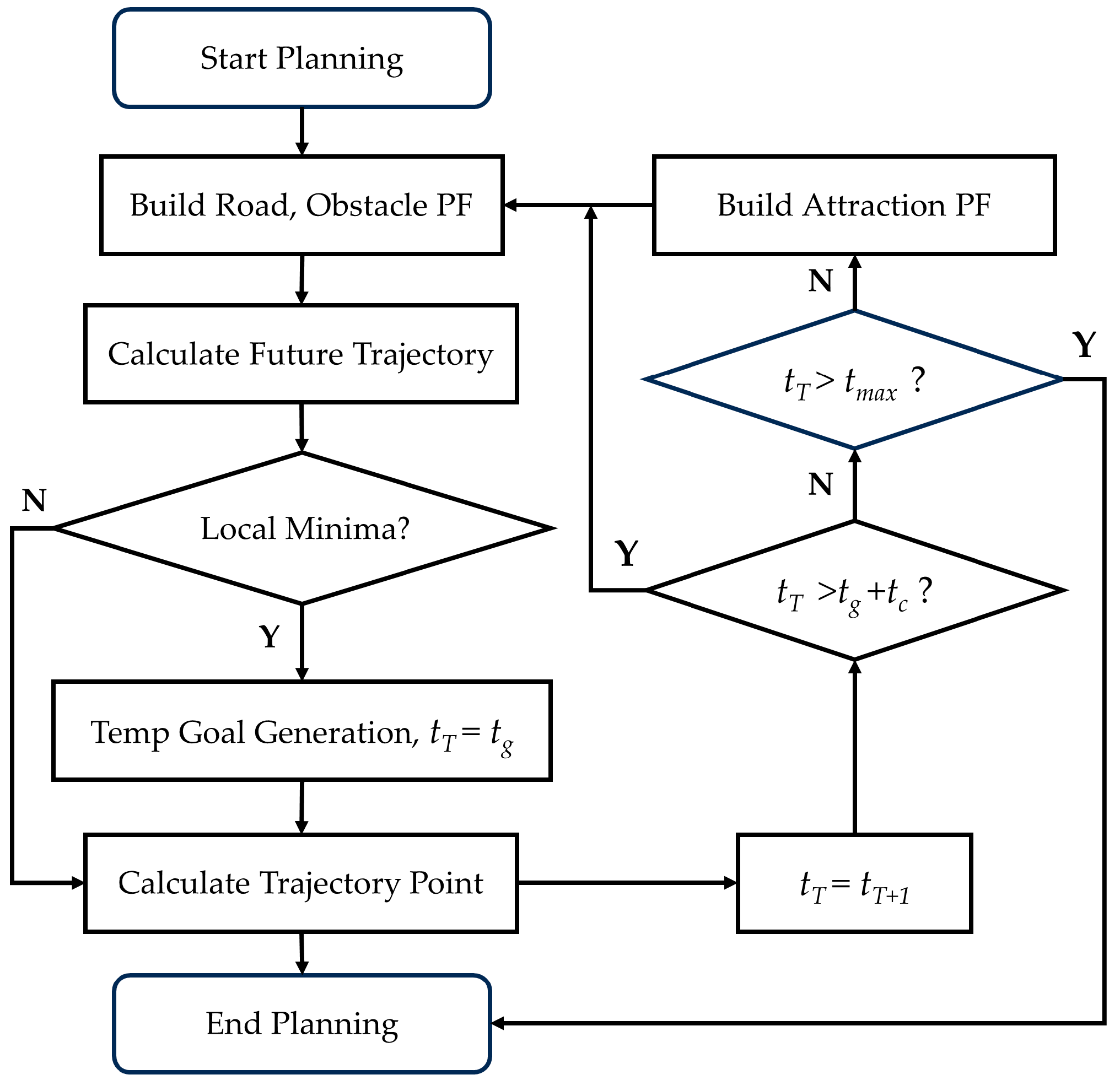
As Figure 6 shows, after initialization, the algorithm will first determine if the vehicle is within the influence range. If the vehicle is within the influence range, the obstacle potential field is subsequently generated using the data from additional sensors. If not, the goal attraction and road boundary fields will be the entire field. The virtual force is obtained in the next step using the total potential field. Next, the velocity is updated based on the virtual force. Lastly, the position point will be calculated using the virtual force and the velocity. In the meantime, we introduce a future prediction process and temporary goal to solve the local minimum problem. The following section shows illustrations showing the specifics of the local minimum and velocity updates.

3.1. Virtual Force Generation

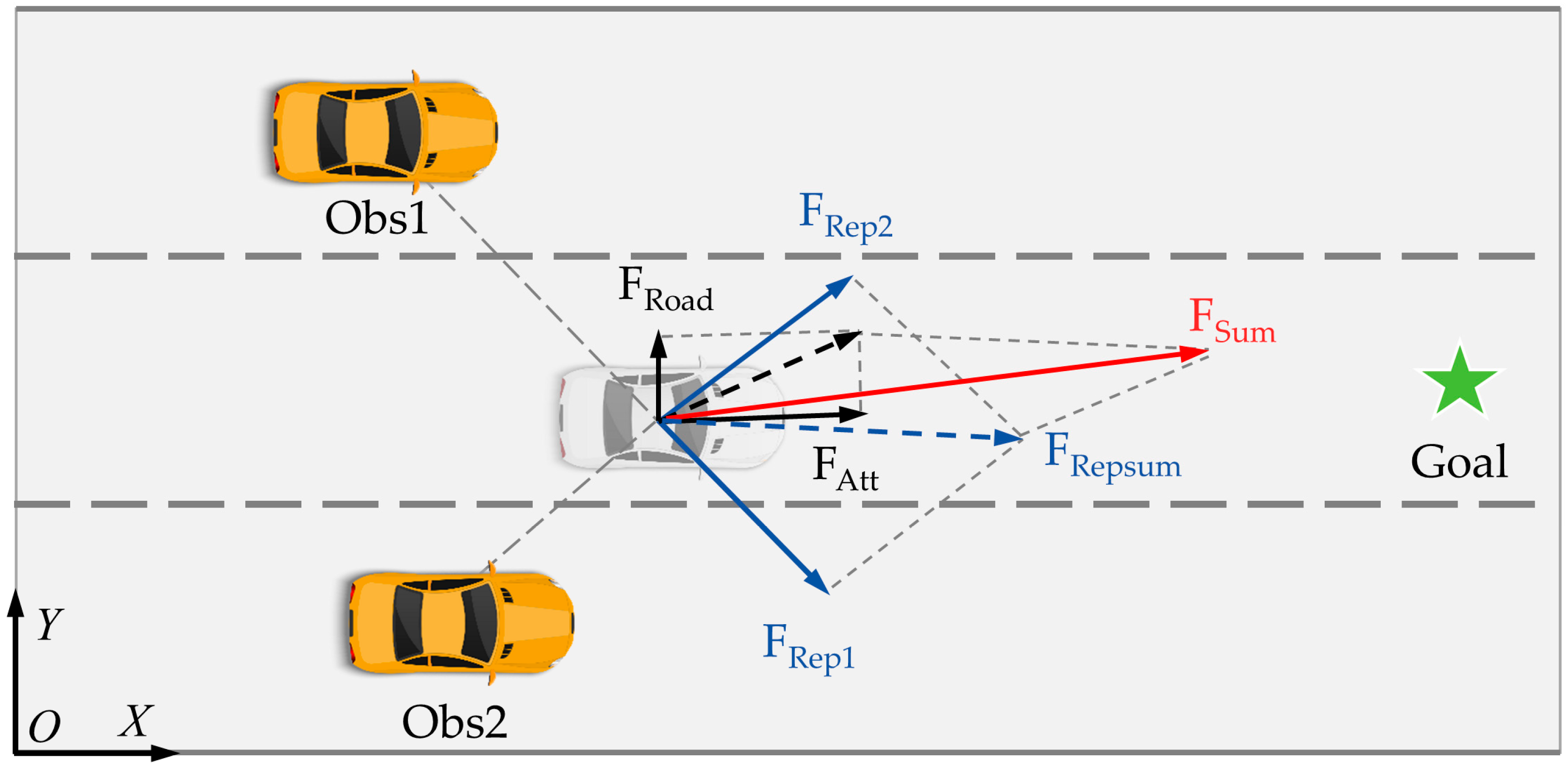
Figure 7 shows the virtual forces are generated using the potential field. The negative gradient of the current position is the virtual force of the potential field. Mathematically, the direction of the negative gradient is the direction where the potential field declines fastest. The expression is as follows:

$$F=-\nabla U_{Total}=(F_X,F_Y)=(-\frac{\partial U_{Total}}{\partial X},-\frac{\partial U_{Total}}{\partial Y})$$

(13)

where U_Total is the sum of all potential fields; F_X and F_Y are the X and Y components of virtual force, respectively.

In programming practices, the virtual force can be computed directly without building the environment’s potential field, which can shorten the method’s computation time. Using (4)–(13), the following functions are derived:

For the force along the x-axis:

$$F_X=-\frac{\partial U_{Total}}{\partial X}=-\frac{\partial (U_{Road}+U_{Goal}+U_{Obs})}{\partial X}=-b_2-\frac{\partial U_{Obs}}{\partial X}$$

(14)

The only variable is the obstacle; the derivative of the obstacle potential field is:

$$\frac{\partial U_{Obs}}{\partial X}=[\frac{G_R{G}_{\cos }[{(y-y_o)}^2+{(x-x_o)}^2]+(y-y_o)G_{\sin }}{{(y-y_o)}^2+{(x-x_o)}^2}]e^{A_x{R}_x{}^2+A_y{R}_y{}^2}$$

(15)

$$\left\{\begin{array}{l}{G}_{\cos }=\cos (\arctan \left(\frac{y-y_o}{x-x_o}\right))\\ G_{\sin }=\sin (\arctan \left(\frac{y-y_o}{x-x_o}\right))\\ G_{Rx}=2A_x{R}_x\cos \phi +2A_y{R}_y\sin \phi \\ G_{Ry}=2A_y{R}_y\cos \phi -2A_x{R}_x\sin \phi \end{array}\right.$$

(16)

For the lateral force in the Y-direction:

$$F_Y=-\frac{\partial U_{Total}}{\partial Y}=-\frac{\partial (U_{Road}+U_{Goal}+U_{Obs})}{\partial Y}$$

(17)

$$\frac{\partial U_{Road}}{\partial Y}=\left\{\begin{array}{l}4k_1(Y-d_w){}^3,2d_w\ge Y>\frac{3d_w}{2}\\ -2k_2(d_w-Y),\frac{3d_w}{2}\ge Y>d_w\\ 2k_2(d_w-Y),d_w\ge Y>\frac{d_w}{2}\\ -4k_1{Y}^3,\frac{d_w}{2}\ge Y\ge 0\end{array}\right.$$

(18)

$$\frac{\partial U_{Goal}}{\partial Y}=\frac{\pi }{d_w}{b}_3\sin (\frac{\pi }{Y-Y_0+D_g}(Y-Y_0))$$

(19)

$$\frac{\partial U_{Obs}}{\partial Y}=[\frac{G_{Ry}*G_{\cos }*[{(y-y_o)}^2+{(x-x_o)}^2]+(x-x_o)G_{\sin }}{{(y-y_o)}^2+{(x-x_o)}^2}]*e^{A_x{R}_x{}^2+A_y{R}_y{}^2}$$

(20)

By adding the derivatives, the calculation can be minimized, which helps the algorithm to be calculated in real-time speed.

Using the virtual force, the expected heading angle φ_E is calculated in the following equation:

$${\phi }_E=\arctan (\frac{\mathit{F}}{‖\mathit{F}‖})$$

(21)

The position point of the next time step will be updated using the equation as follows:

$$\begin{array}{l}\left\{\begin{array}{l}{X}_{n+1}=X_n+\cos {\phi }_E*v_c*t\\ Y_{n+1}=Y_n+\sin {\phi }_E*v_c*t\end{array}\right.\\ \end{array}$$

(22)

In (21), X_n and Y_n are the position coordinate values of the current step; X_n+1 and Y_n+1 are the position coordinate values of the next step; v_c is the velocity after the velocity update process. The velocity update process will be discussed in Section 3.3.

3.2. Future Prediction Mechanism to Solve Local Minimum

In the traditional APF method, the vehicle will come to a halt and remain stationary in the environment when a local minimum point is reached, where the combined virtual force acting on it is zero. It is a limitation of the APF method due to its design theory.

The definition of local minimum in traditional APF is where the sum of virtual forces equals zero:

$$F=-\nabla U_{Total}=0$$

(23)

As a result, in the traditional APF approach, which does not take the velocity into consideration, the host vehicle will stop at the local minimum point.

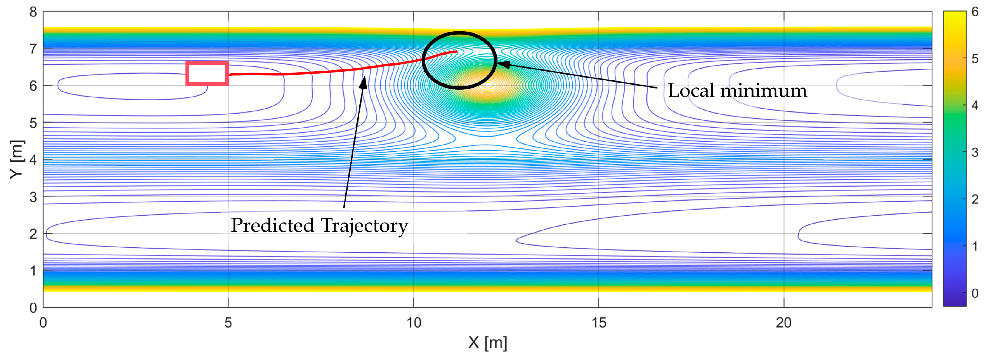
During the planning phase of this article, this approach considers the fact that the vehicle will maintain a consistently high velocity throughout the driving process. As a result, the vehicle’s speed prevents it from consistently remaining stationary at the local minimum position. However, the local minimum point will still attract the host vehicle and lead to an infeasible trajectory. As Figure 8 shows, the predicted trajectory shows how the local minimum drags the vehicle to the road boundary. In real-world driving practice, it is unacceptable to plan a trajectory that hits the road boundary and then go back to the lane.

To address this issue, the proposed method introduces a future prediction process that predicts thefuture movement of the host vehicle using the motion statew. At each time step, the algorithm will calculate the movement in the future in low resolution. The future prediction result can be utilized to judge whether the vehicle will be trapped into the local minimum point:

$$Loca{l}_{Future}={\displaystyle \sum _{k=1}^{n}sign((y_{t_k}-}\frac{(y_{nb}+y_{lc})}{2}))$$

(24)

where y_nb, y_lc is the Y-axis coordinate of the nearest road boundary of the vehicle and the center of the current lane. Equation (24) shows how the Algorithm 1 decides whether the vehicle will be trapped in a local minimum. Specifically, the algorithm counts all points that are stuck between the obstacle and the road boundary. If the Local_Future is larger than the predefined sensitivity parameter C_f, the vehicle will be judged that it will be trapped in the local minimum in the future.

Algorithm 1. Local minimum calculation

Input: Current state of the vehicle (x, y, v, φ), road geometry (ynb, ylc), obstacle (x, y, v, φ)

Output: Temporary goal Ygoal, Flag indicates whether the vehicle will enter the local minimum Step 1: Calculate the future movement of the obstacle and vehicle in low resolution. Step 2: $Loca{l}_{Future}={\displaystyle \sum _{k=1}^{n}sign((y_{t_k}-}\frac{(y_{nb}+y_{lc})}{2}))$ Step 3: If LocalFuture > Cf, Flag =1, otherwise Flag =0. Step 4: If Flag =1, $Y_{goal}=y_{lc}-d_w*sign(y-y_b)$, Tg =t; otherwise continue. Step 5: Calculate goal attraction force by the effect of temporary goal Step 6: If t= Tg +Tc1, Flag = 0.

1Tc is the predefined time that the temporary goal lasts.

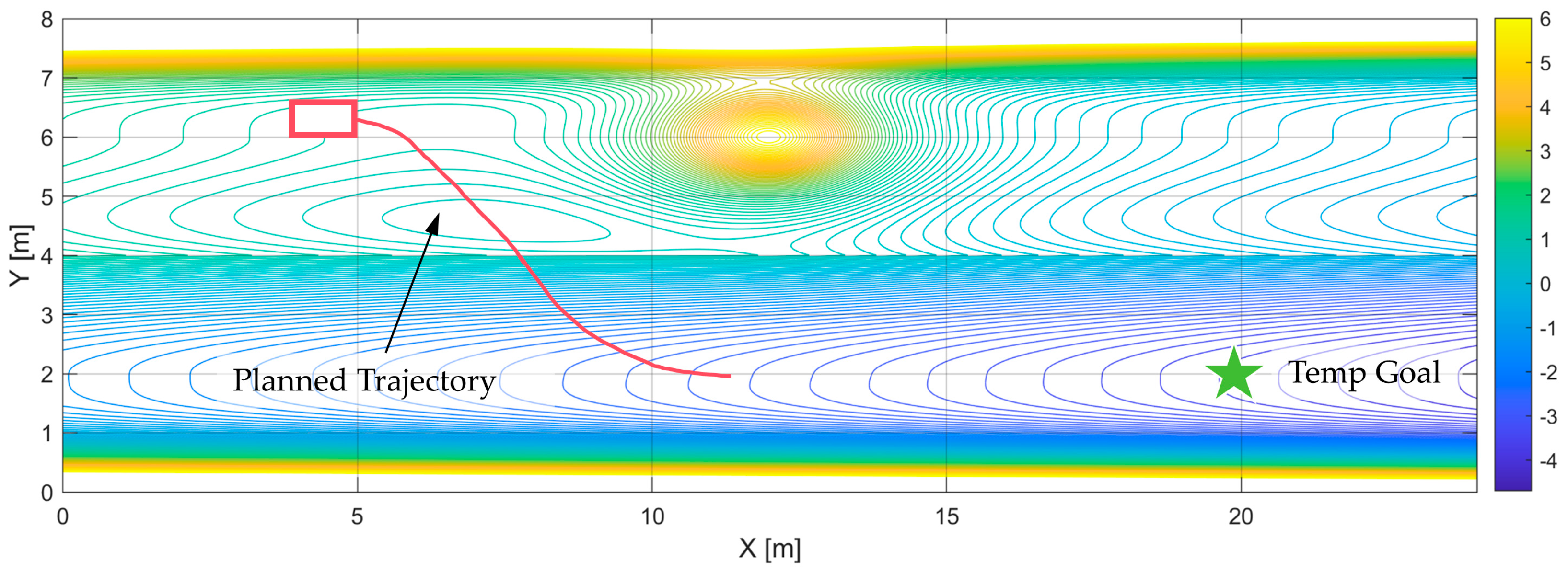
As Figure 9 shows, when a local minimum is detected, the algorithm will generate a temporary goal to place an attractive force on the vehicle to drive out of the local minimum. The temporary goal will exist for a limited time to ensure that it will not affect the movement of vehicles later. When a temporary goal exists, the upper lane’s PF value is much larger than the lower one. According to (8), the PF value will decline smoothly to guide the vehicle to the goal lane.

3.3. Velocity Update

During the algorithm initialization step of the planning process, the cruise velocity V_c is determined. In essence, the vehicle obeys the following rules: when there are no other cars nearby, maintain the cruise speed, accelerate when passing, and decelerate to the speed of the obstacle when following.

The velocity update mechanism is introduced to enable the vehicle to follow the obstacle car. In detail, the velocity update step using the part of F_sum in x direction F_ox to guide the calculation of acceleration.

The following is how the velocity updates:

$$a_v=\frac{{\eta }_1{F}_{ox}+{\eta }_2{(v_c-V_c)}^3}{m}$$

(25)

$$v_c=v_b+at$$

(26)

where v_b is the velocity of the step before, and v_c is the velocity of the current step. Vc is the cruising speed set at the initialization. The granularity of the result is determined by the planning time step of the entire algorithm. The host vehicle’s mass is represented by m. The force magnitude is controlled by the parameter η₁. The parameter that regulates the vehicle’s return to its cruising speed is η₂.

After introducing the acceleration and velocity update mechanism, the improved APF method is able to accelerate when passing and decelerate to the speed of the obstacle when following. In the end, the method will plan a trajectory that is more like human-driving logic.

It is obvious that the future calculation mechanism and velocity update will add extra calculation burden to the improved APF.

Table 1. Parameter settings in the simulation.

Parameters	Value	Parameters	Value
k1	3.397	vobs1.1	18 km/h
k2	5.809	vobs1.2	18 km/h
dw	4 m	vobs1.3	28.8 km/h
b1	20	aobs1	6 m/s2
b2	0.15	yobs1.1	1.8 m
b3	1.52	yobs1.2	5.5 m
Ax	−0.15	yobs1.3	1.9 m
Ay	−0.2	vobs2.1	28.8 km/h
η1	0.63	vobs2.2	32.4 km/h
η2	0.25	vobs2.3	27 km/h
t	0.02 s	vobs2.4	28.8 km/h
T	5 s	vobs2.5	25.2 km/h
Sm	5 m	yobs2.1	5.7 m
ab	6 m/s2	yobs2.2	2 m
Fstep 1	20	yobs2.3	5.7 m
Cf	5	yobs2.4	6 m
Tc	0.4 s	yobs2.5	6 m

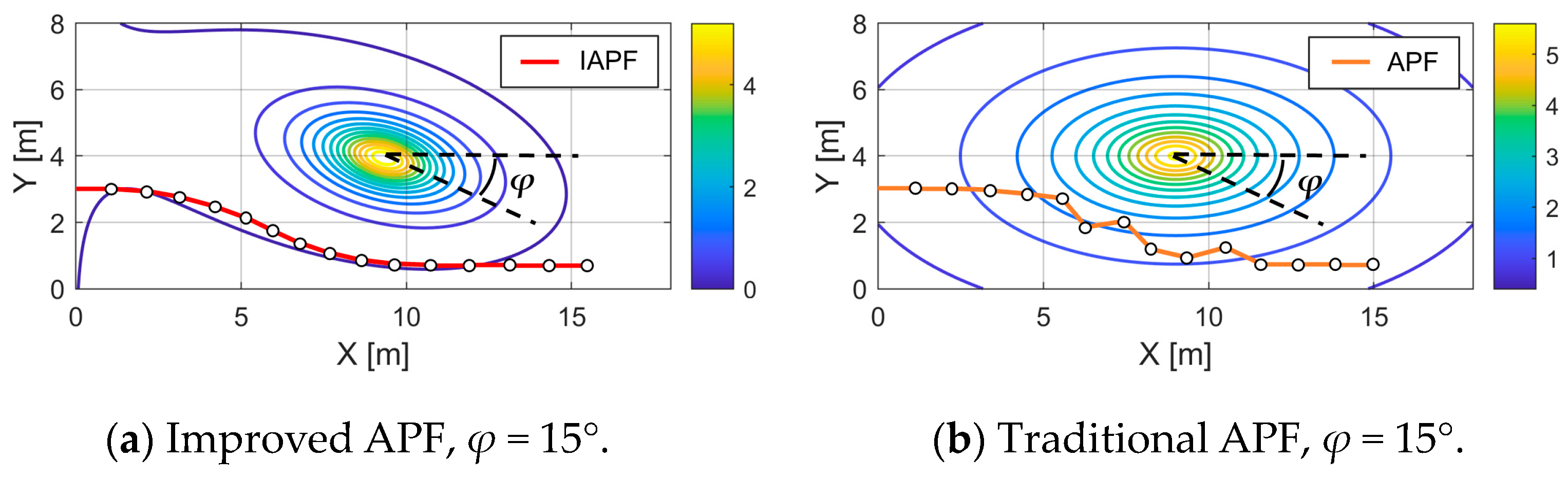
¹ F_step is the future steps calculated in the future prediction process.

gives the results that after adding this mechanism, the algorithm indeed takes more time to finish the whole planning task, but the maximum heading angle is decreasing, which indicates that the trajectory planned by improved APF is smoother than the traditional APF method. At the same time, the velocity is able to change based on the actual driving situation.

4. Simulation and Result Analysis

4.1. Simulation Environment

In this section, the simulations are performed in MATLAB R2020a environment using a computer with Intel Xeon W-2245 CPU and 64 GB RAM. First, a long driving scenario, which can be divided into three cases on a standard city road, is given to verify the effectiveness of the proposed method. In time sequence, the cases are static obstacle avoidance, dynamic obstacle with the local minimum, and car following. Then, a complex and challenging scenario is given to prove the ability of the algorithm to handle heavy traffic.

The road geometry is the standard one-way road with two lanes. It is worth noting that the speed is generally limited to below 40 km/h on urban roads in China’s traffic regulations and traffic environment. Hence, the speed of the host vehicle is assigned as 36 km/h.

In the first long-driving scenario, there are three obstacle vehicles in this scenario. Obstacle 1 starts with 18 km/h and decelerates at t = 0 s; Obstacle 2 also starts with 18 km/h; Obstacle 3 starts with 28.8 km/h and accelerates at t = 16 s with a = 2 m/s². The whole simulation ends at t = 20 s.

In the second complex scenario, there are five obstacles in total. Horizontally, the velocities of the vehicles are 28.8 km/h, 32.4 km/h, 27 km/h, 28.8 km/h, and 25.2 km/h, respectively. All obstacle vehicles are moving at a constant speed. Obstacle 4 will take the lane change maneuver at t = 5.5 s to t = 8.3 s.

The detailed simulation parameters are given in Table 1. Note that the parameters in Table 1 are one possible expression based on our hyperparameter tuning through a number of simulations.

4.2. Simulation Result

4.2.1. Case A: Static Obstacle Avoidance

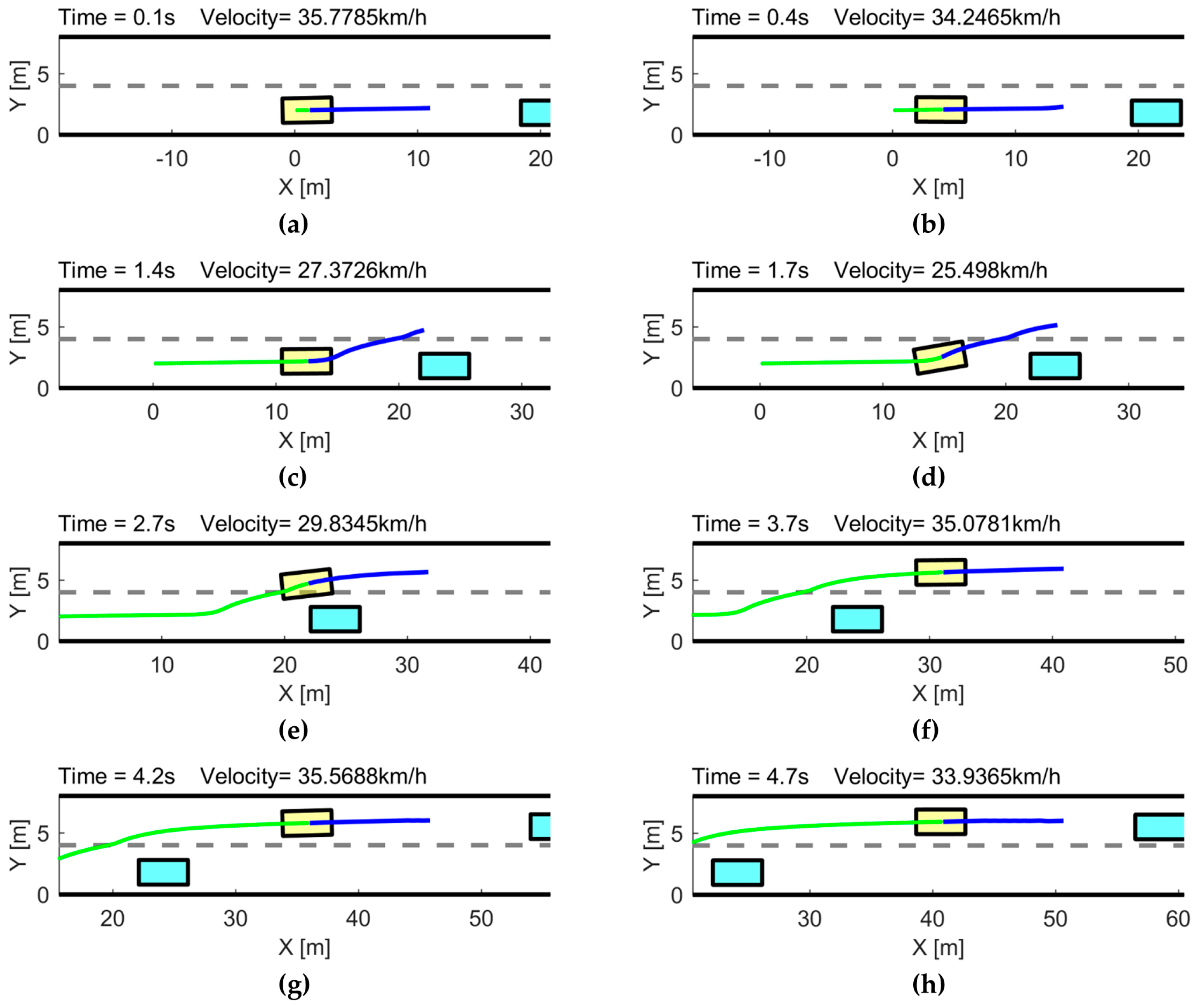
As Figure 10 shows, at the beginning of this case, the host vehicle is driving along the road at the speed of 36 km/h. the obstacle vehicle is in the front of the host vehicle.

At the same time, the front vehicle starts to decelerate rapidly to 0 m/s. At the beginning, as Figure 10b,c show, the host vehicle is trying to decelerate to follow the front vehicle. After deceleration, the host vehicle finds out it cannot follow the vehicle, and then it starts a lane change maneuver. Figure 10d,e show how the vehicle changes lanes to avoid any potential collision. In Figure 10f,g, the vehicle is accelerated to a cruising speed of 36 km/h. In summary, the proposed method is able to handle the static obstacle avoidance scenario.

4.2.2. Case B: Dynamic Obstacle with Local Minimum

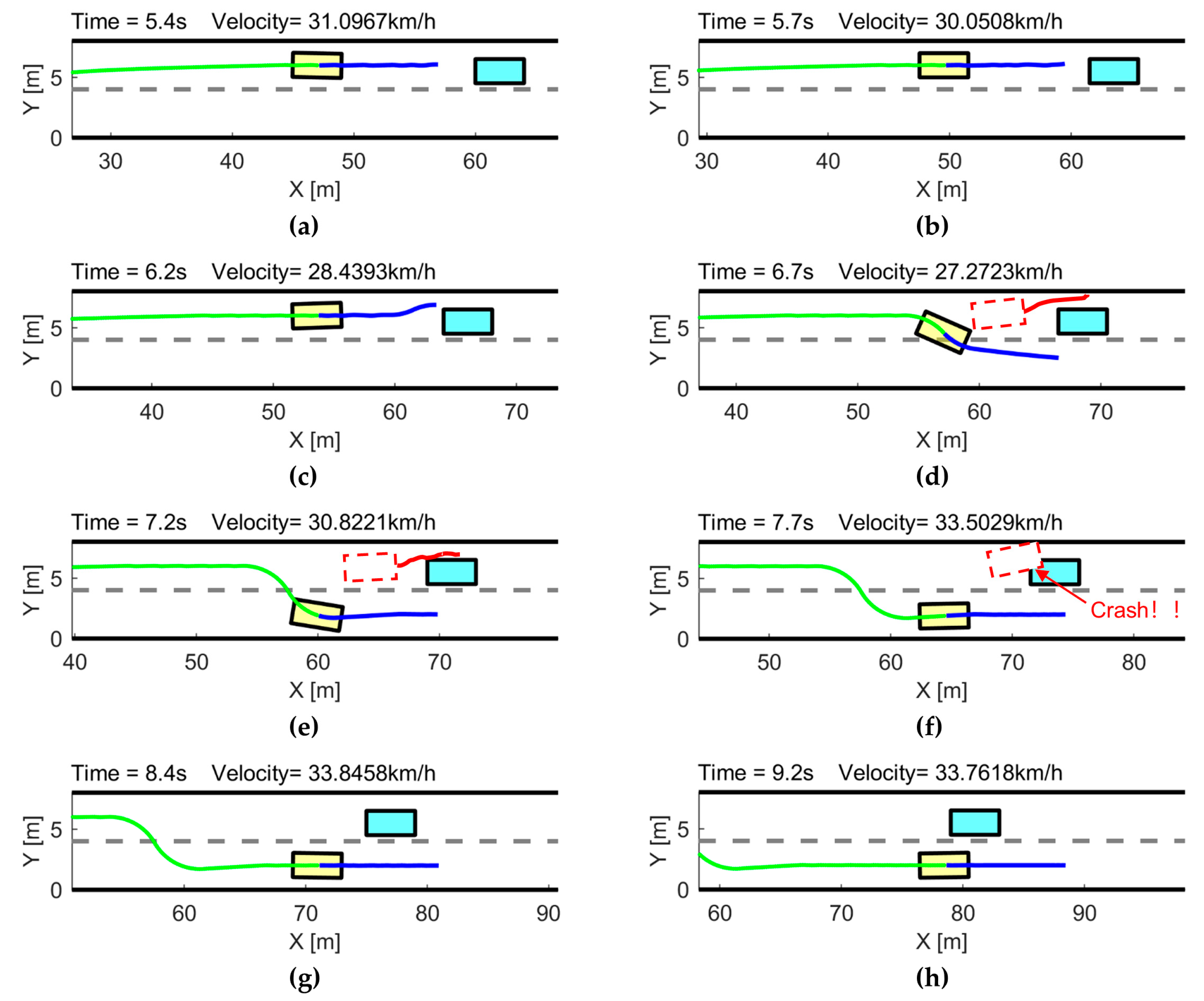
After overtaking the static obstacle, the next obstacle moves in the road at 18 km/h. As Figure 11b,c show, after approaching the obstacle, the future detection head is stuck into the local minimum. If you keep driving along the future prediction result, the vehicle will crash into the road boundary or the obstacle vehicle. Figure 11d–f show the planning result of traditional APF which will cause crash accidents. As Figure 11d–f show, when the local minimum is detected, the algorithm will generate a temporary goal point to place an attractive force to guide the movement of the host vehicle. It is obvious that Figure 11d shows how the attractive force drags the vehicle to another lane. As a result, in Figure 11f–h, the host vehicle drives out of the local minimum and cruises on the road.

4.2.3. Case C: Car following

In this case, the obstacle vehicle is moving at a speed of 28.8 km/h, which is close to the cruising speed of the host vehicle. Here, the host vehicle is decelerating to follow the front car, and as Figure 12f shows, the host vehicle follows the car successfully and decelerates to 30.8 km/h.

Here, the red car in Figure 12b–f shows how the traditional APF will react in the car in the following case. Due to the lack of a velocity update process, the traditional APF method will always try to avoid collision by lane-changing. The proposed method can decelerate to follow the obstacle vehicle.

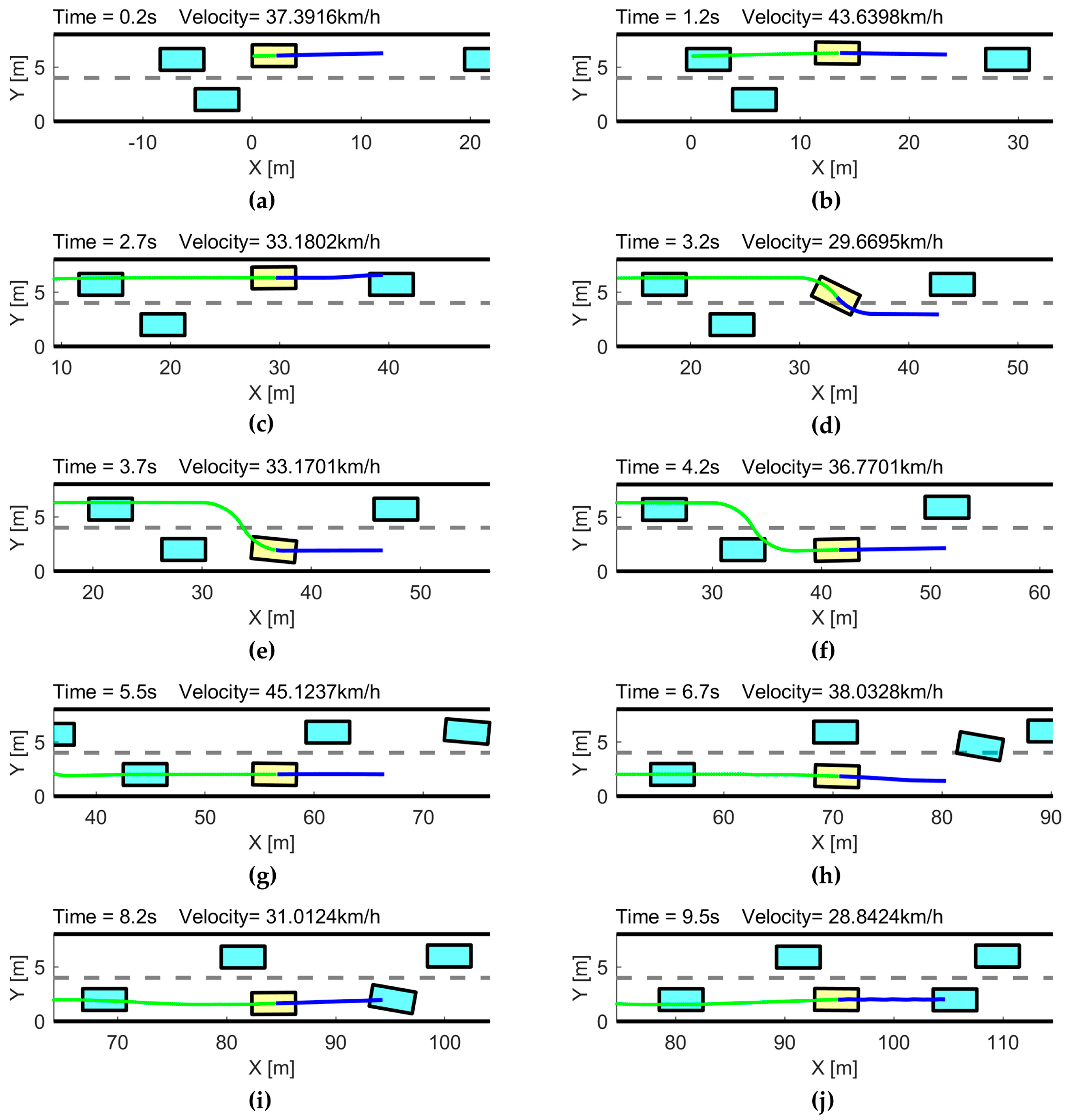
4.2.4. Case D: Complex Scenario

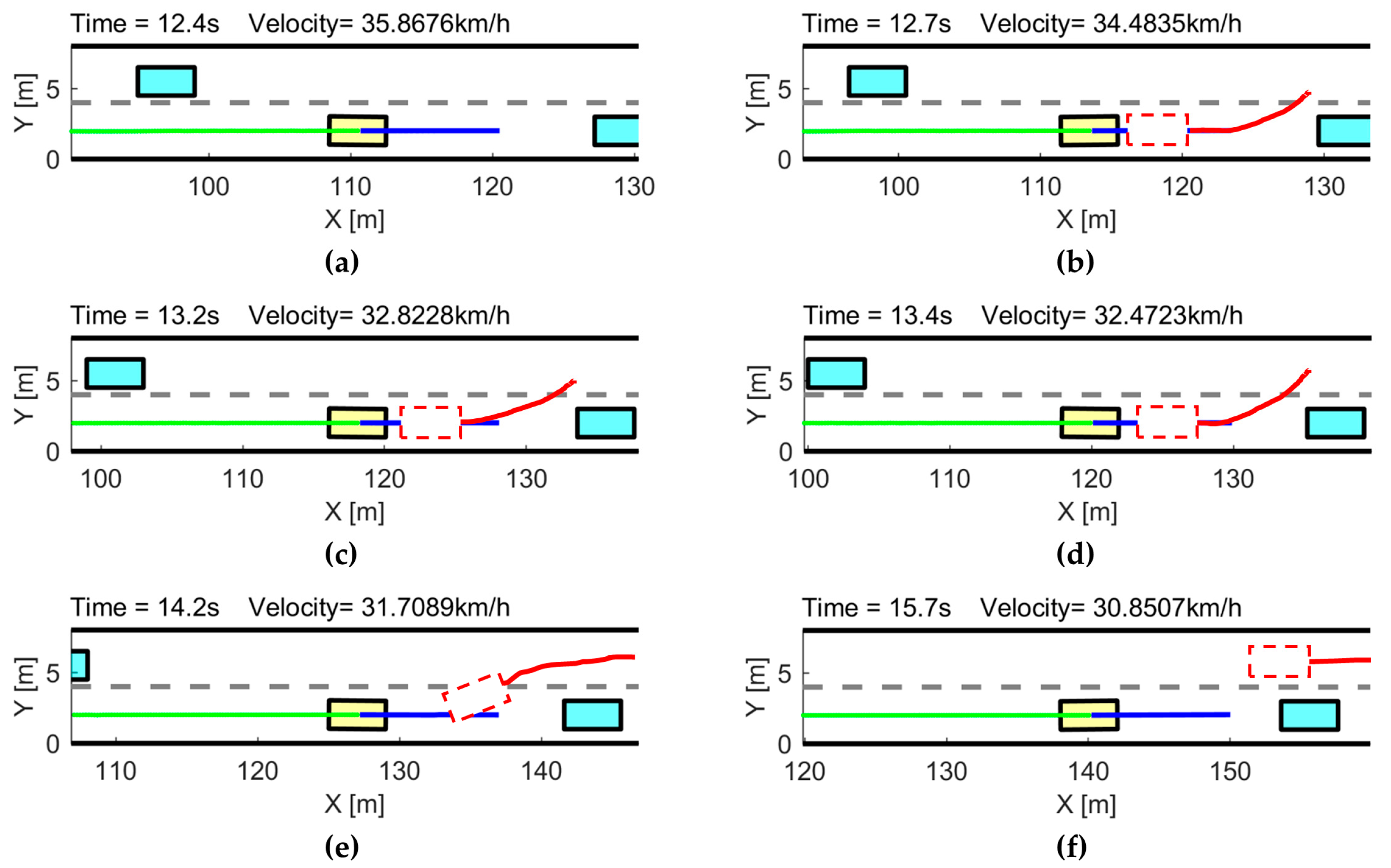
For simplicity, the obstacles in this case are encoded based on the sequence in the X-axis. For example, in Figure 13a, the obstacle vehicle in the back of the host vehicle is obstacle 1.

In this case, the host vehicle is driving in the heavy traffic. First, by the influence of the obstacle in the back, the host vehicle accelerates to keep a safe distance from the obstacle. Later, as shown in Figure 13c, the host vehicle is decelerating owing to the influence of obstacle 3. At the same time, the future prediction mechanism detects a local minimum, which will potentially generate an infeasible trajectory. In Figure 13d, a temporary goal is generated to guide the host vehicle to change the lane. As Figure 13h shows, obstacle 4 is taking the lane change maneuver because of the slow obstacle 5. By the influence of the rotation factor, the vehicle instantly reacts to the obstacle 4′s behavior and starts to decelerate. At the end of the simulation, the host vehicle is cruising in the traffic stream.

4.3. Computation Time Cost Analysis

As shown in

Table 2. Contrast between the proposed method and traditional APF.

Simulations	Case Time	1 Case Calculation Time	2 Time Range
IAPF-Case A	5 s	0.233 s	4.130–4.809 ms
IAPF-without prediction-Case A	5 s	0.181 s	3.589–3.771 ms
APF-Case A	5 s	0.167 s	3.312–3.397 ms
IAPF-Case B	5 s	0.225 s	4.072–4.629 ms
IAPF-Case C	6 s	0.233 s	3.666–4.129 ms
IAPF-Case D	10 s	0.476 s	4.541–4.969 ms

¹ Case calculation time is the total calculation time in each case at planning frequency = 0.1 s; ² time range indicates the maximum and minimum of single planning at a time horizon T = 5 s.

, the computation time of improved APF and improved APF-without prediction is acceptably larger than the traditional APF in Case A. The future prediction will add extra computation cost to the proposed method. It is worth noting that the maximum time cost of improved APF (≈200 Hz) is efficient enough and can achieve real-time planning (>20 Hz).

5. Conclusions

To enhance the trajectory-planning performance of autonomous ground vehicles, this paper proposes an efficient trajectory-planning approach based on the improved artificial potential field method. By incorporating the carefully designed potential fields, future prediction mechanism, and velocity update process, the proposed improved artificial potential field planning approach is able to plan a smooth, collision-free trajectory. Three cases in the simulation are given to prove the performance difference between the proposed method and traditional APF and the effectiveness of the improved artificial potential field planning approach. In the future, we will further research motion planning of the input inaccurate problem caused by imperfect sensors and conduct experiments in real autonomous ground vehicles.

References

1. Claussmann, L.; Revilloud, M.; Gruyer, D.; Glaser, S. A Review of Motion Planning for Highway Autonomous Driving. IEEE Trans. Intell. Transp. Syst. 2020, 21, 1826–1848. [Google Scholar] [CrossRef]
2. González, D.; Pérez, J.; Milanés, V.; Nashashibi, F. A Review of Motion Planning Techniques for Automated Vehicles. IEEE Trans. Intell. Transp. Syst. 2016, 17, 1135–1145. [Google Scholar] [CrossRef]
3. Jiang, C.; Wang, C.; Wang, M. Research on path planning for mobile robots based on improved A-star algorithm. In Proceedings of the IEEE 7th Information Technology and Mechatronics Engineering Conference (ITOEC), Chongqing, China, 15–17 September 2023; pp. 723–727. [Google Scholar]
4. Zhang, Z.; Wang, S.; Zhou, J. A-star algorithm for expanding the number of search directions in path planning. In Proceedings of the 2nd International Seminar on Artificial Intelligence, Networking and Information Technology (AINIT), Shanghai, China, 15–17 October 2021; pp. 208–211. [Google Scholar]
5. Yang, H.; Li, H.; Liu, K.; Yu, W.; Li, X. Research on path planning based on improved RRT-Connect algorithm. In Proceedings of the 33rd Chinese Control and Decision Conference (CCDC), Kunming, China, 22–24 May 2021; pp. 5707–5712. [Google Scholar]
6. Li, X.; Tong, Y. Path Planning of a Mobile Robot Based on the Improved RRT Algorithm. Appl. Sci. 2024, 14, 25. [Google Scholar] [CrossRef]
7. Wang, X.; Liu, J.; Peng, H. A Simultaneous Planning and Control Method Integrating APF and MPC to Solve Autonomous Navigation for USVs in Unknown Environments. Intell. Robot. Syst. 2022, 105, 36. [Google Scholar] [CrossRef]
8. Jiaming, F.; Xia, C.; Xiao, L. UAV trajectory planning based on bi-directional APF-RRT* algorithm with goal-biased. Expert Syst. Appl. 2023, 213, 119–137. [Google Scholar]
9. Sepehri, A.; Moghaddam, A.M. A motion planning algorithm for redundant manipulators using rapidly exploring randomized trees and artificial potential fields. IEEE Access 2021, 9, 26059–26070. [Google Scholar] [CrossRef]
10. Fernandes, P.B.; Oliveira, R.C.L.; Neto, J.V.F. Trajectory planning of autonomous mobile robots applying a particle swarm optimization algorithm with peaks of diversity. Appl. Soft Comput. 2022, 116, 108108. [Google Scholar] [CrossRef]
11. Liu, C.; Lee, S.; Varnhagen, S.; Tseng, H.E. Path planning for autonomous vehicles using model predictive control. In Proceedings of the IEEE Intelligent Vehicles Symposium (IV), Redondo Beach, CA, USA, 11–14 June 2017; pp. 174–179. [Google Scholar]
12. Yao, Q.; Zheng, Z.; Qi, L. Path planning method with improved artificial potential field—A reinforcement learning perspective. IEEE Access 2020, 8, 135513–135523. [Google Scholar] [CrossRef]
13. Feng, S.; Qian, Y.; Wang, Y. Collision avoidance method of autonomous vehicle based on improved artificial potential field algorithm. Proc. Inst. Mech. Eng. D J. Autom. Eng. 2021, 235, 3416–3430. [Google Scholar] [CrossRef]
14. Sun, Y.; Chen, W.; Lv, J. UAV Path Planning Based on Improved Artificial Potential Field Method. In Proceedings of the International Conference on Computer Network, Electronic and Automation (ICCNEA), Xi’an, China, 23–25 September 2022; pp. 95–100. [Google Scholar]
15. Bounini, F.; Gingras, D.; Pollart, H.; Gruyer, D. Modified artificial potential field method for online path planning applications. In Proceedings of the IEEE Intelligent Vehicles Symposium (IV), Redondo Beach, CA, USA, 11–14 June 2017; pp. 180–185. [Google Scholar]
16. Luo, J.; Wang, Z.; Pan, K. Reliable Path Planning Algorithm Based on Improved Artificial Potential Field Method. IEEE Access 2022, 10, 108276–108284. [Google Scholar] [CrossRef]
17. Li, H. Robotic Path Planning Strategy Based on Improved Artificial Potential Field. In Proceedings of the International Conference on Artificial Intelligence and Computer Engineering (ICAICE), Beijing, China, 23–25 October 2020; pp. 67–71. [Google Scholar]
18. Wahid, N.; Zamzuri, H.; Amer, N.H. Collision avoidance motion planning strategy using artificial potential field with adaptive multi-speed scheduler. IET Intell. Transp. Syst. 2022, 14, 1200–1209. [Google Scholar] [CrossRef]
19. Narita, Y.; Konaka, E. Design of multiple artificial potential function and selector function for autonomous driving vehicle. In Proceedings of the IEEE International Conference on Consumer Electronics (ICCE), Las Vegas, NV, USA, 10–12 January 2021; pp. 1–5. [Google Scholar]
20. Szczepanski, R.; Tarczewski, T.; Erwinski, K. Energy Efficient Local Path Planning Algorithm Based on Predictive Artificial Potential Field. IEEE Access 2022, 10, 39729–39742. [Google Scholar] [CrossRef]
21. Xie, S.; Hu, J.; Bhowmick, P.; Ding, Z.; Arvin, F. Distributed Motion Planning for Safe Autonomous Vehicle Overtaking via Arti-ficial Potential Field. IEEE Trans. Intell. Transp. Syst. 2022, 23, 21531–21547. [Google Scholar] [CrossRef]
22. Zhe, C.; Bing, X. AGV Path Planning Based on Improved Artificial Potential Field Method. In Proceedings of the IEEE International Conference on Power Electronics, Computer Applications (ICPECA), Shenyang, China, 22–24 January 2021; pp. 32–37. [Google Scholar]
Figure 1. Architecture of proposed planning approach.
Symmetry 16 00106 g001
Figure 2. Standard road structure.
Symmetry 16 00106 g002
Figure 3. Different road fields. (a) The road boundary repulsion field, and (b) the goal attraction field.
Symmetry 16 00106 g003
Figure 4. Obstacle potential field of different vehicles. (a) The smaller the size and mass (b), the larger the size and mass.
Symmetry 16 00106 g004
Figure 5. Obstacle potential field of improved APF and APF method while the heading angle of the obstacle φ = 15°.
Symmetry 16 00106 g005
Figure 6. The planning process of the proposed method.
Symmetry 16 00106 g006
Figure 7. Illustration of virtual force.
Symmetry 16 00106 g007
Figure 8. Local minimum and future prediction.
Symmetry 16 00106 g008
Figure 9. The potential field when a temporary goal is activated.
Symmetry 16 00106 g009
Figure 10. Simulation results of static obstacle avoidance.
Symmetry 16 00106 g010
Figure 11. Simulation results of dynamic obstacle with local minimum. In (df), the red car shows the planning results of traditional APF, which will cause a crash accident.
Symmetry 16 00106 g011
Figure 12. Simulation results of the car following. The red car in (bf) shows the results of traditional APF in the car-following case.
Symmetry 16 00106 g012
Figure 13. Simulation result of a complex scenario.
Symmetry 16 00106 g013