

Toward Enhanced Geological Analysis: A Novel Approach Based on Transmuted Semicircular Distribution

 , ,
, ,  , and
, and 
Abstract
:1. Introduction
2. Definition and Derivation of the Proposed Model
- (i)
- , ,
- (ii)
- ,
- (iii)
- .
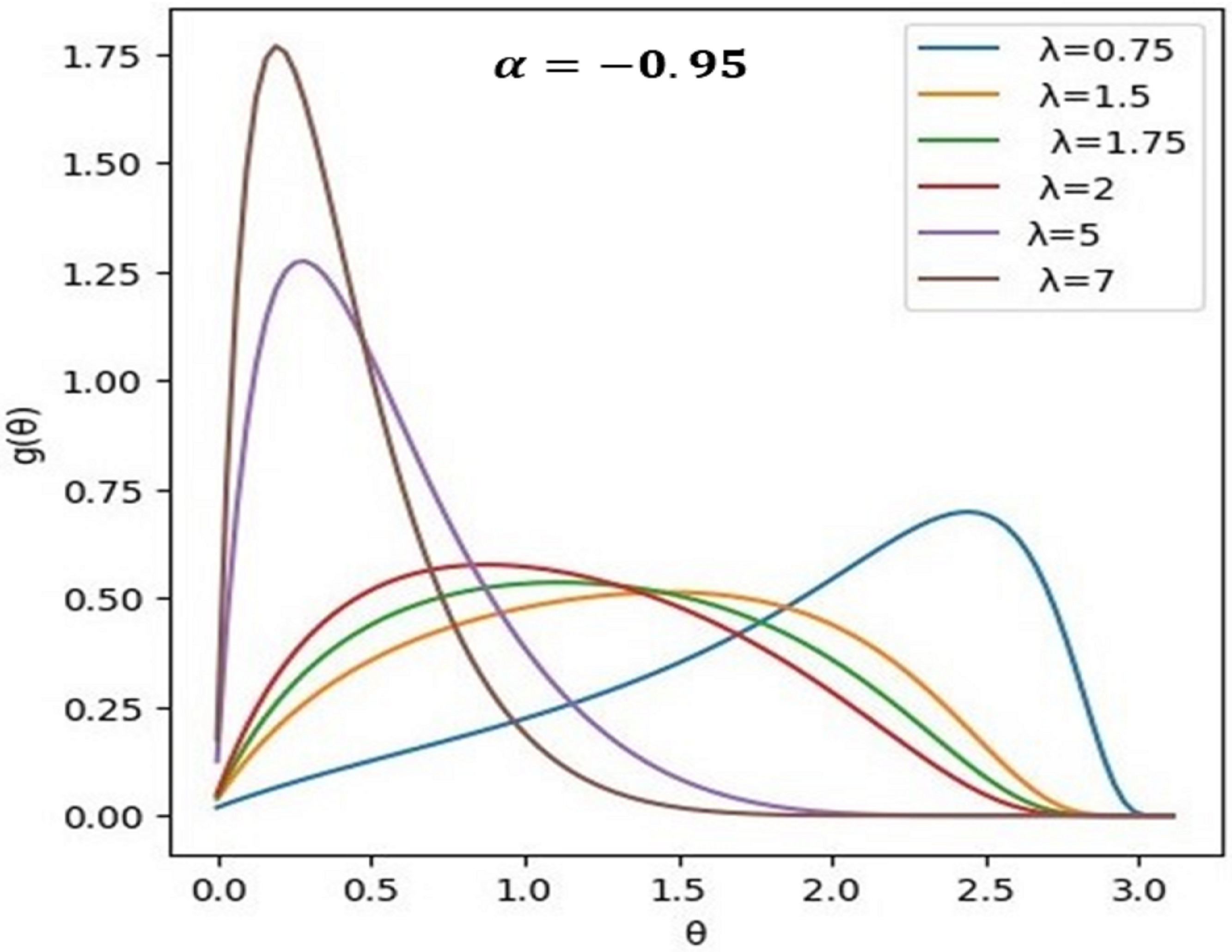
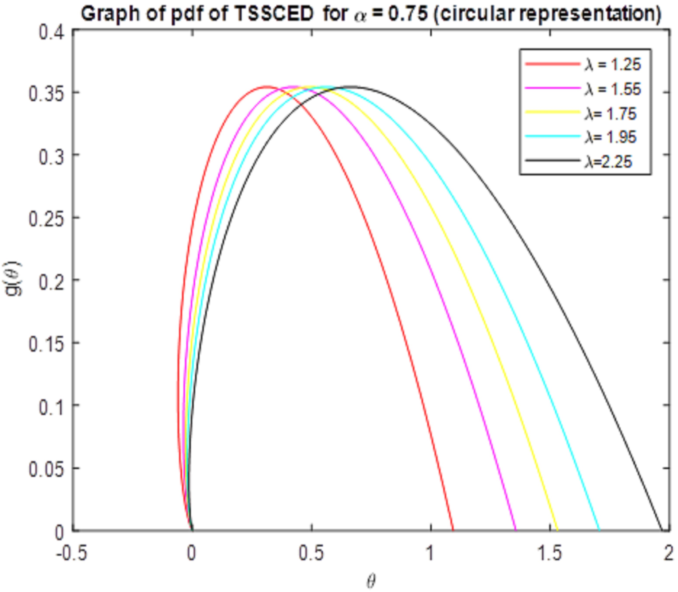
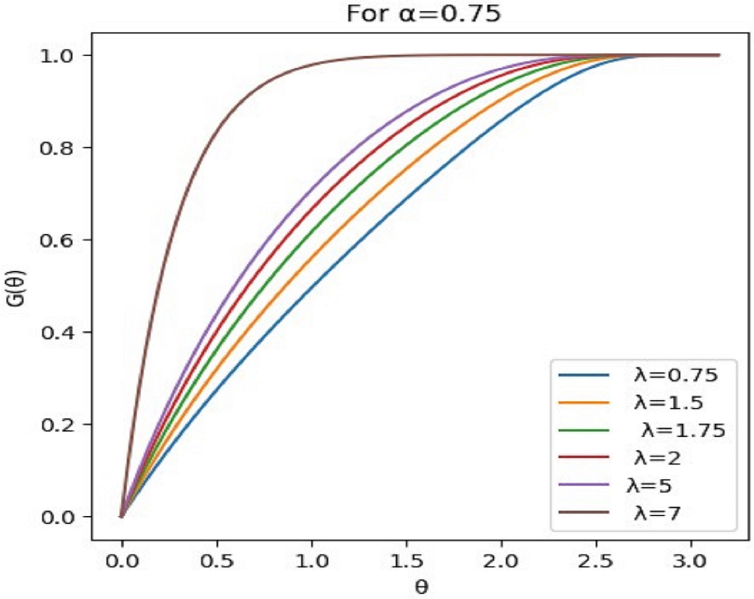
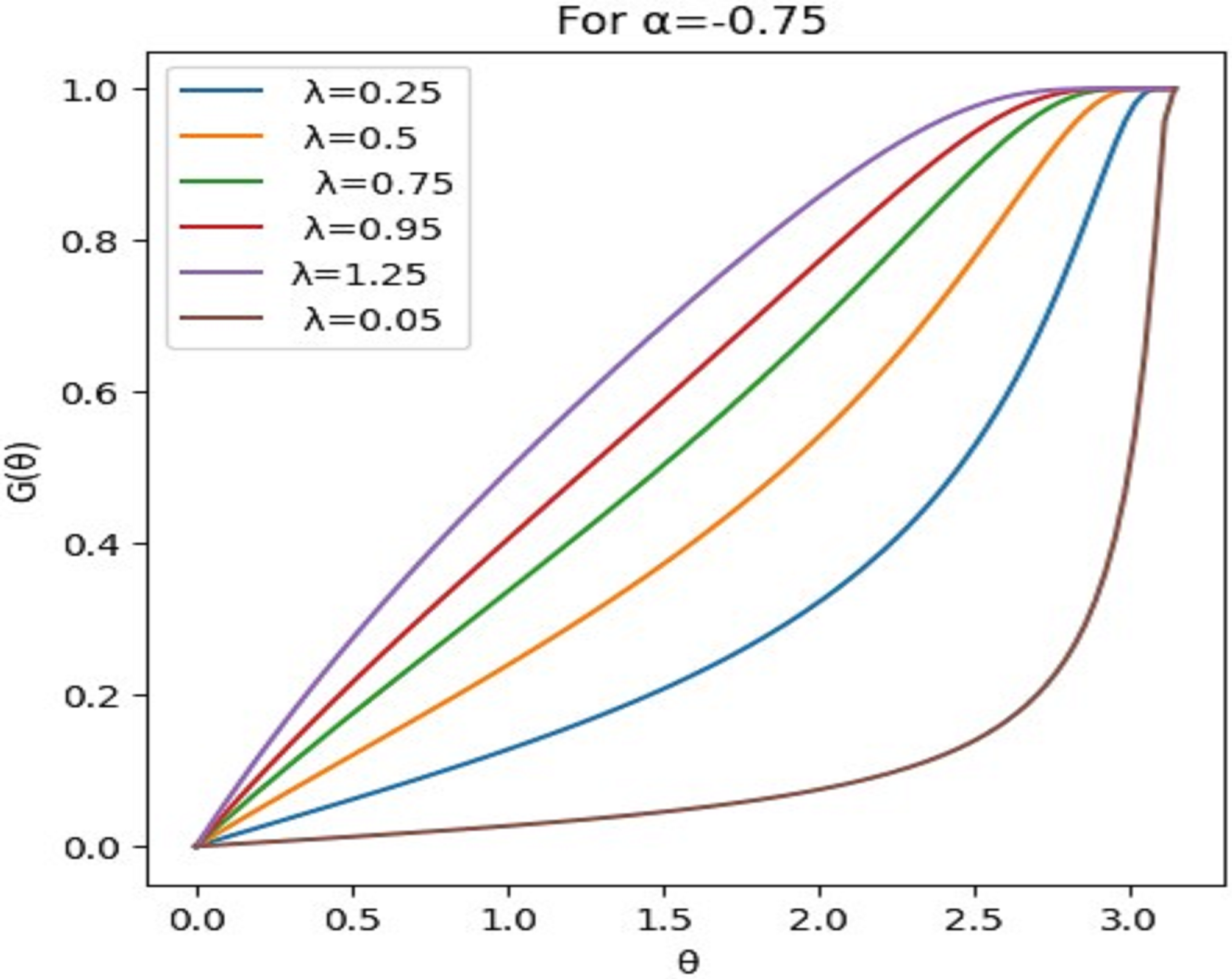
- Transmuted stereographic semicircular exponential distribution (TSSCED)
Quantile Function
3. Characteristic Function
The Trigonometric Moments
4. The Maximum Likelihood Estimation
5. Simulation Study
- Step-I: Generating a random sample from a given distribution;
- Step-(a): A random variable is generated from the U (0, 1) distribution, say u;
- Step-(b): Find the expression for the quantile function for the given distribution (i.e., find the inverse of cumulative distribution function);
- Step-II: Obtain maximum likelihood estimates of the parameters.
- Step-III: Calculate the average bias, MSE, and MRE.
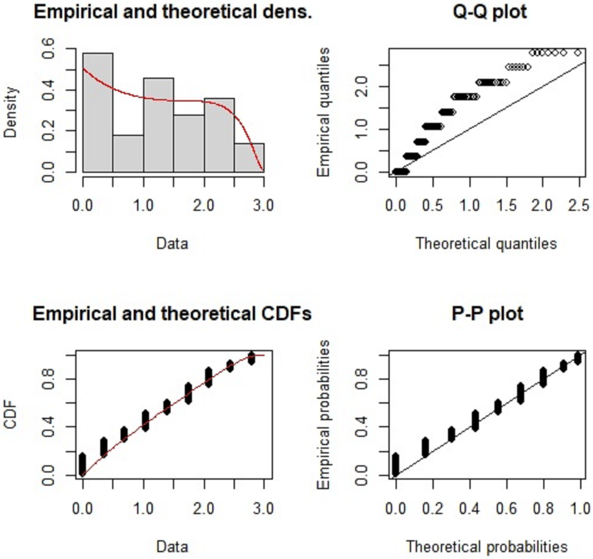
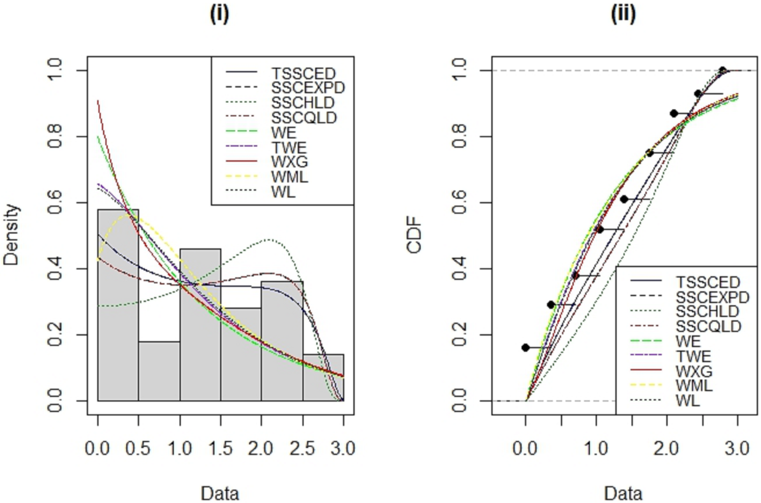
6. Application
7. Conclusions
Author Contributions
Funding
Data Availability Statement
Acknowledgments
Conflicts of Interest
References
- Hamasha, M.M. Practitioner advice: Approximation of the cumulative density of left-sided truncated normal distribution using logistic function and its implementation in Microsoft Excel. Qual. Eng. 2017, 29, 322–328. [Google Scholar] [CrossRef]
- Khan, M.A.; Meetei, M.Z.; Shah, K.; Abdeljawad, T.; Alshahrani, M.Y. Modeling the monkeypox infection using the Mittag–Leffler kernel. Open Phys. 2023, 21, 20230111. [Google Scholar] [CrossRef]
- Kamal, S.; Rohul, A.; Thabet, A. Utilization of Haar wavelet collocation technique for fractal-fractional order problem. Heliyon 2023, 9, e17123. [Google Scholar] [CrossRef]
- Albert, W.M.; Ingram, O. A New Method for Adding a parameter to a family of Distributions with Applications to the Exponential and Weibull Families. Biometrika 1997, 84, 641–652. [Google Scholar]
- Shaw, W.; Buckley, I. The Alchemy of Probability Distributions. Beyond Gram-Charlier Expansions and A Skew-Kurtotic –Normal Distribution from a Rank Transmutation Map. arXiv 2007, arXiv:0901.0434. [Google Scholar] [CrossRef]
- Merovci, F. Transmuted Lindley Distribution. Int. J. Open Probl. Compt. Math. 2013, 6, 64–72. [Google Scholar] [CrossRef]
- Merovci, F.; Ibrahim, E. Transmuted Lindley-geometric distribution and its applications. J. Stat. Appl. Probab. 2014, 3, 77–91. [Google Scholar] [CrossRef]
- Kemaloglu, S.A.; Yilmaz, M. Transmuted two-parameter Lindley distribution. Commun. Stat.-Theory Methods 2017, 46, 11866–11879. [Google Scholar] [CrossRef]
- Rao, J.S.; Gupta, S. Topics in Circular Statistics; World Scientific Press: Singapore, 2001. [Google Scholar]
- Jammalamadaka, S.R.; Kozubowski, T.J. A new family of circular models: The wrapped Laplace distributions. Adv. Appl. Stat. 2003, 3, 77–103. [Google Scholar]
- Jammalamadaka, S.R.; Kozubowski, T.J. New Families of Wrapped distributions for modeling Skew circular data. Commun. Stat.-Theory Methods 2004, 33, 2059–2074. [Google Scholar] [CrossRef]
- Abe, T.; Shimizu, K.; Pewsey, A. Symmetric unimodel models for directional data motivated by inverse stereographic projection. J. Jpn. Stat. Soc. 2020, 40, 45–61. [Google Scholar] [CrossRef]
- Minh, D.L.P.; Farnum, N.R. Using bilinear transformations to induce probability distributions. Commun. Stat.-Theory Methods 2003, 32, 1–9. [Google Scholar] [CrossRef]
- Jones, M.C.; Pewsey, A. A family of symmetric distributions on the circle. J. Am. Stat. Assoc. 2005, 100, 1422–1428. [Google Scholar] [CrossRef]
- Yedlapalli, P.; Girija, S.V.S.; Rao, A.V.D. On Construction of Stereographic Semicircular models. J. Appl. Probab. Stat. 2013, 8, 75–90. [Google Scholar]
- Rao, A.V.D.; Sharma, I.R.; Girija, S.V.S. On wrapped version of some life testing models. Commun. Stat.-Theory Methods 2007, 36, 2027–2035. [Google Scholar] [CrossRef]
- Arnold, B.; Sen, C.; Gupta, A. Probability distributions and statistical inference for axial data. Environ. Ecol. Stat. 2016, 13, 271–285. [Google Scholar] [CrossRef]
- Rambli, A.; Mohamed, I.B.; Shimizu, K.; Khalidin, N. Outlier detection in a new half-circular distribution. In Proceedings of the AIP Conference Proceedings, Selangor, Malaysia, 24–26 November 2015; p. 050018. [Google Scholar] [CrossRef]
- Ali, H.A. A half circular distribution for modeling the posterior corneal curvature. Commun. Stat.-Theory Methods 2017, 47, 3118–3124. [Google Scholar] [CrossRef]
- Rambli, A.; Mohamed, I.B.; Shimizu, K.; Khalidin, N. A Half-Circular Distribution on a Circle. Sains Malays. 2019, 48, 887–892. [Google Scholar] [CrossRef]
- Abdullah, Y.; Cenker, B. A new wrapped exponential distribution. Math. Sci. 2018, 12, 285–293. [Google Scholar] [CrossRef]
- Yedlapalli, P.; Girija, S.V.S.; Akkayajhula, V.D.R.; Sastry, K.L.N. On Stereographic Semicircular Quasi Lindley Distribution. J. New Results Sci. (JNRS) 2016, 8, 6–13. [Google Scholar]
- Yedlapalli, P.; Subrahmanyam, P.S.; Girija, S.V.S.; Rao, A.V.D. Stereographic Semicircular Half Logistic Distribution. Int. J. Pure Appl. Math. (IJPAM) 2017, 113, 142–150. [Google Scholar]
- Yedlapalli, P.; Girija, S.V.S.; Rao, A.V.D.; Sastry, K.L.N. A New Family of Semicircular and Circular Arc Tan-Exponential Type Distributions. Thai J. Math. 2020, 18, 775–781. [Google Scholar]
- Ayesha, I.; Azeem, A.; Hanif, M. Half circular modified burr-III distribution, application with different estimation methods. PLoS ONE 2022, 17, e0261901. [Google Scholar] [CrossRef]
- Alldredge, J.R.; Mahtab, M.A.; Panek, L.A. Statistical analysis of axial data. J. Geol. 1974, 82, 519–524. [Google Scholar] [CrossRef]
- Mardia, K.V.; Jupp, P.E. Directional Statistics, 2nd ed.; John Wiley Sons, Ltd.: Hoboken, NJ, USA, 2000. [Google Scholar]
- Gradshteyn, R. Table of Integrals, Series and Products, 7th ed.; Academic Press: Cambridge, MA, USA, 2007. [Google Scholar]
- Krumbein, W.C. Preferred Orinetation of Pebbles in Sedimentary Deposits. J. Geol. 1939, 47, 673–706. [Google Scholar] [CrossRef]
- Joshi, S.; Jose, K.K. Wrapped Lindley Distribution. Commun. Stat.-Theory Methods 2018, 47, 1013–1021. [Google Scholar] [CrossRef]
- Al-Mofleh, H.; Sen, S. The wrapped xgamma distribution for modeling circular data appearing in geological context. arXiv 2019, arXiv:1903.00177. [Google Scholar] [CrossRef]
- Christophe, C.; Lishamol, T.; Meenu, J. Wrapped modified Lindley distribution. J. Stat. Manag. Syst. 2021, 24, 1025–1040. [Google Scholar]
- Boulila, W.; Farah, I.; Ettabaa, K.; Solaiman, B.; Ghézala, H. Improving spatiotemporal change detection: A high level fusion approach for discovering uncertain knowledge from satellite image databases. Icdm 2009, 9, 222–227. [Google Scholar]
- Ferchichi, A.; Boulila, W.; Farah, I. Propagating aleatory and epistemic uncertainty in land cover change prediction process. Ecol. Inform. 2017, 37, 24–37. [Google Scholar] [CrossRef]


| Sample Size | ||||||||
|---|---|---|---|---|---|---|---|---|
| n | ||||||||
| n | MLE | Bias | MSE | MRE | MLE | Bias | MSE | MRE |
| 20 | −0.30923 | 0.42563 | 0.25468 | −1.70253 | 1.53668 | 0.37243 | 0.24245 | 0.24829 |
| 40 | −0.25845 | 0.3390 | 0.17890 | −1.35599 | 1.55175 | 0.30226 | 0.17154 | 0.20151 |
| 100 | −0.23798 | 0.23241 | 0.09592 | −0.92964 | 1.54459 | 0.20985 | 0.09844 | 0.13990 |
| 200 | −0.24235 | 0.16354 | 0.04966 | −0.65415 | 1.52372 | 0.14304 | 0.04808 | 0.09536 |
| 900 | −0.25044 | 0.07357 | 0.00858 | −0.29429 | 1.50136 | 0.06098 | 0.00595 | 0.04065 |
| n | ||||||||
| MLE | Bias | MSE | MRE | MLE | Bias | MSE | MRE | |
| 20 | −0.71745 | 0.27163 | 0.13031 | −0.36217 | 2.07549 | 0.37501 | 0.28395 | 0.18751 |
| 40 | −0.73827 | 0.20850 | 0.07905 | −0.27800 | 2.04035 | 0.26774 | 0.15105 | 0.13387 |
| 100 | −0.74988 | 0.13439 | 0.02934 | −0.17918 | 2.00860 | 0.16353 | 0.04483 | 0.08177 |
| 200 | −0.75048 | 0.09666 | 0.0149 | −0.12888 | 2.00517 | 0.11410 | 0.02079 | 0.05705 |
| 900 | −0.75002 | 0.04551 | 0.00326 | −0.06067 | 2.00106 | 0.05308 | 0.00446 | 0.02654 |
| n | ||||||||
| MLE | Bias | MSE | MRE | MLE | Bias | MSE | MRE | |
| 20 | 0.06332 | 0.46435 | 0.32862 | 1.85741 | 2.60236 | 0.6671 | 0.65624 | 0.24258 |
| 40 | 0.11763 | 0.38189 | 0.21671 | 1.52758 | 2.66402 | 0.59805 | 0.53040 | 0.21747 |
| 100 | 0.19594 | 0.29615 | 0.12576 | 1.18460 | 2.76669 | 0.50778 | 0.39994 | 0.18465 |
| 200 | 0.23879 | 0.23884 | 0.08486 | 0.95537 | 2.75853 | 0.42811 | 0.30909 | 0.15568 |
| 900 | 0.25602 | 0.19277 | 0.05951 | 0.77109 | 2.75097 | 0.35724 | 0.23727 | 0.12991 |
| n | ||||||||
| MLE | Bias | MSE | MRE | MLE | Bias | MSE | MRE | |
| 20 | 0.3497 | 0.43623 | 0.31876 | 0.87246 | 3.32569 | 0.75798 | 0.81984 | 0.21657 |
| 40 | 0.38084 | 0.36559 | 0.21933 | 0.73117 | 3.38228 | 0.70477 | 0.69674 | 0.20136 |
| 100 | 0.41406 | 0.29573 | 0.13587 | 0.59146 | 3.42742 | 0.63041 | 0.55988 | 0.18012 |
| 200 | 0.44827 | 0.24924 | 0.09391 | 0.49849 | 3.46991 | 0.56018 | 0.44954 | 0.16005 |
| 900 | 0.48967 | 0.16542 | 0.04037 | 0.33083 | 3.51229 | 0.39465 | 0.23494 | 0.11276 |
| n | ||||||||
| MLE | Bias | MSE | MRE | MLE | Bias | MSE | MRE | |
| 20 | 0.61623 | 0.36033 | 0.23862 | 0.48044 | 4.44351 | 0.95696 | 1.31564 | 0.20146 |
| 40 | 0.66202 | 0.29647 | 0.14938 | 0.39530 | 4.56807 | 0.85815 | 1.03825 | 0.18066 |
| 100 | 0.69448 | 0.23836 | 0.08797 | 0.31781 | 4.68178 | 0.77811 | 0.84347 | 0.16381 |
| 200 | 0.70655 | 0.20618 | 0.06435 | 0.27490 | 4.71495 | 0.71606 | 0.71555 | 0.15075 |
| 900 | 0.74987 | 0.14159 | 0.03241 | 0.18879 | 4.70835 | 0.50387 | 0.38176 | 0.10608 |
| n | ||||||||
| MLE | Bias | MSE | MRE | MLE | Bias | MSE | MRE | |
| 20 | 0.84397 | 0.15603 | 0.12359 | 0.15603 | 5.31865 | 1.19575 | 2.13013 | 0.19929 |
| 40 | 0.87742 | 0.12258 | 0.07097 | 0.12258 | 5.47974 | 0.97930 | 1.51715 | 0.16322 |
| 100 | 0.90301 | 0.09699 | 0.04792 | 0.09699 | 5.58728 | 0.74017 | 0.99825 | 0.12336 |
| 200 | 0.92618 | 0.07382 | 0.03465 | 0.07382 | 5.69486 | 0.55759 | 0.67826 | 0.09293 |
| 900 | 0.97800 | 0.02200 | 0.00591 | 0.02200 | 5.88721 | 0.22750 | 0.13504 | 0.03792 |
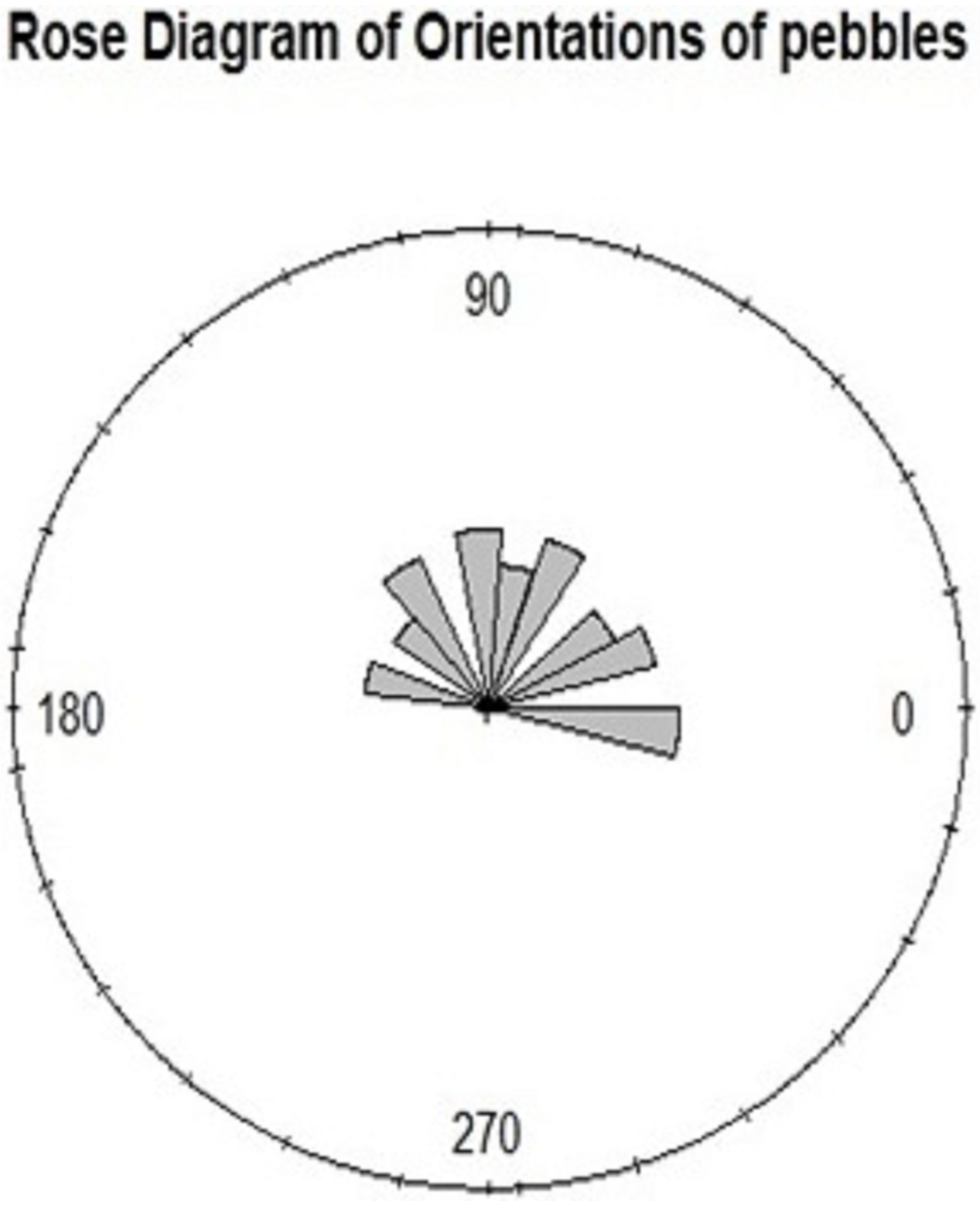
| Direction | 0 | 20 | 40 | 60 | 80 | 100 | 120 | 140 | 160 |
| Frequency | 16 | 13 | 9 | 14 | 9 | 14 | 12 | 6 | 7 |
| Model | (SE) | (SE) |
|---|---|---|
| WE () | 0.7925781 (0.08714681) | – |
| TWE () | 0.9076947 (0.1091980 ) | −0.2786174 (0.1737912) |
| SSCEXPD () | 0.8707031 (0.0870702) | – |
| TSSCED () | 0.6486455 (0.1179918) | 0.5616030 (0.2311657) |
| SSCHLD () | 0.8724609 (0.07618154) | – |
| SSCQLD () | 37.410889 (114.4836132) | 0.8929941 (0.11080331) |
| WRXG () | 1.506348 (0.1119663) | – |
| WML () | 0.8916573 (0.07748228) | – |
| WL () | 1.181641 (0.09453908) | – |
| Model | LL | AIC | CAIC | BIC | HQIC | KS (p-Value) |
|---|---|---|---|---|---|---|
| TSSCED () | −103.8731 | 211.7461 | 211.8698 | 216.9565 | 213.8449 | 0.146 (0.06598) |
| SSCEXPD () | −106.4283 | 214.8566 | 214.8974 | 217.4617 | 215.9109 | 0.16 ( 0.03195) |
| WE () | −119.1116 | 240.2282 | 240.624 | 242.8284 | 241.2776 | 0.27892 (0.00003) |
| TWE () | −188.1661 | 240.3323 | 240.456 | 245.5426 | 242.441 | 0.169 (0.006355) |
| SSCLHD () | −115.5355 | 233.071 | 233.1118 | 235.6762 | 234.1254 | 0.20069 (0.0006346) |
| SSCQLD () | −106.4473 | 216.8946 | 217.0183 | 222.105 | 219.0033 | 0.16 (0.1195) |
| WRXG () | −114.8499 | 231.6999 | 231.7407 | 234.3051 | 232.7543 | 0.1823 (0.002597) |
| WML () | −121.4082 | 244.8164 | 244.8572 | 247.4215 | 245.8707 | 0.16 (0.01195) |
| WL () | −117.3191 | 236.6382 | 236.679 | 239.2434 | 237.6926 | 0.16419 (0.009111) |
Disclaimer/Publisher’s Note: The statements, opinions and data contained in all publications are solely those of the individual author(s) and contributor(s) and not of MDPI and/or the editor(s). MDPI and/or the editor(s) disclaim responsibility for any injury to people or property resulting from any ideas, methods, instructions or products referred to in the content. |
© 2023 by the authors. Licensee MDPI, Basel, Switzerland. This article is an open access article distributed under the terms and conditions of the Creative Commons Attribution (CC BY) license (https://creativecommons.org/licenses/by/4.0/).
Share and Cite
Yedlapalli, P.; Kishore, G.N.V.; Boulila, W.; Koubaa, A.; Mlaiki, N. Toward Enhanced Geological Analysis: A Novel Approach Based on Transmuted Semicircular Distribution. Symmetry 2023, 15, 2030. https://doi.org/10.3390/sym15112030
Yedlapalli P, Kishore GNV, Boulila W, Koubaa A, Mlaiki N. Toward Enhanced Geological Analysis: A Novel Approach Based on Transmuted Semicircular Distribution. Symmetry. 2023; 15(11):2030. https://doi.org/10.3390/sym15112030
Chicago/Turabian StyleYedlapalli, Phani, Gajula Naveen Venkata Kishore, Wadii Boulila, Anis Koubaa, and Nabil Mlaiki. 2023. "Toward Enhanced Geological Analysis: A Novel Approach Based on Transmuted Semicircular Distribution" Symmetry 15, no. 11: 2030. https://doi.org/10.3390/sym15112030