1. Introduction
Over the past several years, the efficient computing of matrix functions has emerged as a prominent area of research. Symmetry plays a significant role in the study of matrix functions, particularly in understanding their properties, behavior, and computational methods. Symmetry principles are widely used in physics and engineering to analyze and solve problems involving matrix functions. For instance, in quantum mechanics, symmetric matrices often arise in the context of Hamiltonians, and efficient computation of matrix functions is crucial for simulating quantum systems and predicting their behavior. In order to compute matrix functions, various iterative schemes have been suggested, which include methods for the evaluation of matrix sign function. The scalar sign function defined for
such that
which is given as,
is extended to form the matrix sign function. Roberts [
1] introduced the Cauchy integral representation of the matrix sign function in 1980, given by
which can be applied in model reduction and in solving algebraic Riccati and Lyapunov equations. Recall the definition of matrix sign function
via the Jordan canonical form [
2], in which if
is the Jordan decomposition of
A such that
, then
where
has no eigenvalue on the imaginary axis,
P is a nonsingular matrix, and
p and
are sizes of Jordan blocks
,
corresponding to eigenvalues lying in left half plane
and right half plane
, respectively.
In the pursuit of evaluating
as a solution of
Roberts applied Newton’s method (
) resulting into the following iterative formula:
with the initial matrix
and convergence of order two.
Another alternative is accelerated Newton’s method (
) that can be achieved via norm scaling parameter in (
5) given by,
In order to improve the convergence, acceleration and scaling of iteration (
5), Kenney and Laub [
3,
4] suggested a family of matrix iterations by employing the Padé approximant to the function
where
and taking into the consideration
Let
-Padé approximant to
with
is denoted as
, then
converges to
if
and it has convergence rate equal to
. So, the
-Padé approximant iteration (
) for computing
is
These iterations were later investigated by Gomilko et al. [
5]. Other popular iterative approaches for
, such as the Newton-Schulz method
[
6]
and Halley’s method
[
2]
are either members of the Padé family (
10) or its reciprocal family.
A recent fifth order iterative method [
7] (represented as Lotfi’s Method (
)) for
can be investigated and is given by
For more recent literature on matrix sign function, one can go through references [
8,
9,
10].
Motivated by constructing efficient iterative methods like the methods discussed above and to overcome on some of the drawbacks of the existing iterative methods, here we aim to propose a globally convergent iterative method for approximation of
. Matrix sign function has several application in scientific computing (see e.g., [
11,
12]). Another applications of matrix sign function include solving various matrix equations [
13], solving stochastic differential equations [
14] and many more.
In this article, we present a fifth order iterative scheme for evaluation of
. The outline for the rest of the article is defined here: In
Section 2, the construction of new iterative scheme for evaluating matrix sign function has been concluded. In
Section 3, basins of attraction guarantees the global convergence of developed method. Also, convergence analysis for the fifth rate of convergence is discussed along with stability analysis. Then the proposed method is extended to determine the generalized eigenvalues of a regular matrix pencil in
Section 4. Computational complexity is examined in
Section 5. Numerical examples are provided to evaluate the performance and to demonstrate the numerical precision of suggested method in
Section 6. The final conclusion is presented in
Section 7.
2. A Novel Iterative Method
In this section, we have developed an iterative method for evaluation of
. The primary goal is to develop the scheme by examining the factorization patterns and symmetry of existing schemes rather than using a non-linear equation solver [
13]. We aim to design an iterative formula that does not conflict with the Padé family members (
9) or its reciprocals.
If we assume the eigenvalues to converge to 1 or
, and we aim to get a higher convergence order five, then the iterative formula will satisfy the equation
If we solve Equation (
14) for
, then we get
Nevertheless, the formula mentioned above is not a novel one, as it is a member of Padé family (
9). So, we make some modifications in (
14) so that the formula becomes better in terms of converegnce as follows:
provided that
. Solving (
16) for
, we get
which contains a polynomial of degree 5 in the numerator and a polynomial of degree 6 in the denominator. From (9), it is clear that Padé family has a unique member with a polynomial of degree
in numerator and a polynomial of degree
in denominator for each
. So
and
will result into
and
, i.e.,
and will have order
which is different from the order 5 that we are achieving. So, the above formula (
17) is not a part of the family (
9) or reciprocals of (
9) and therefore our proposed method (
) is as follows:
where
is the appropriate initial guess which we discuss in
Section 3.
Remark 1. Convergence can be slow if for some l. In that situation, it is advisable to introduce the scaling parameter [15] given as,to speed up the convergence [16] of the scheme. Hence, we also present the accelerated proposed method (
) which is accelerated version of (
18) given by
where
and
.
3. Convergence and Stability Analysis
In this section, we discuss the convergence analysis to ensure that the sequence generated from (
18) converges to
for a matrix
. We draw the basins of attraction to confirm the global convergence of the proposed scheme and compared with the existing schemes for solving
[
17].
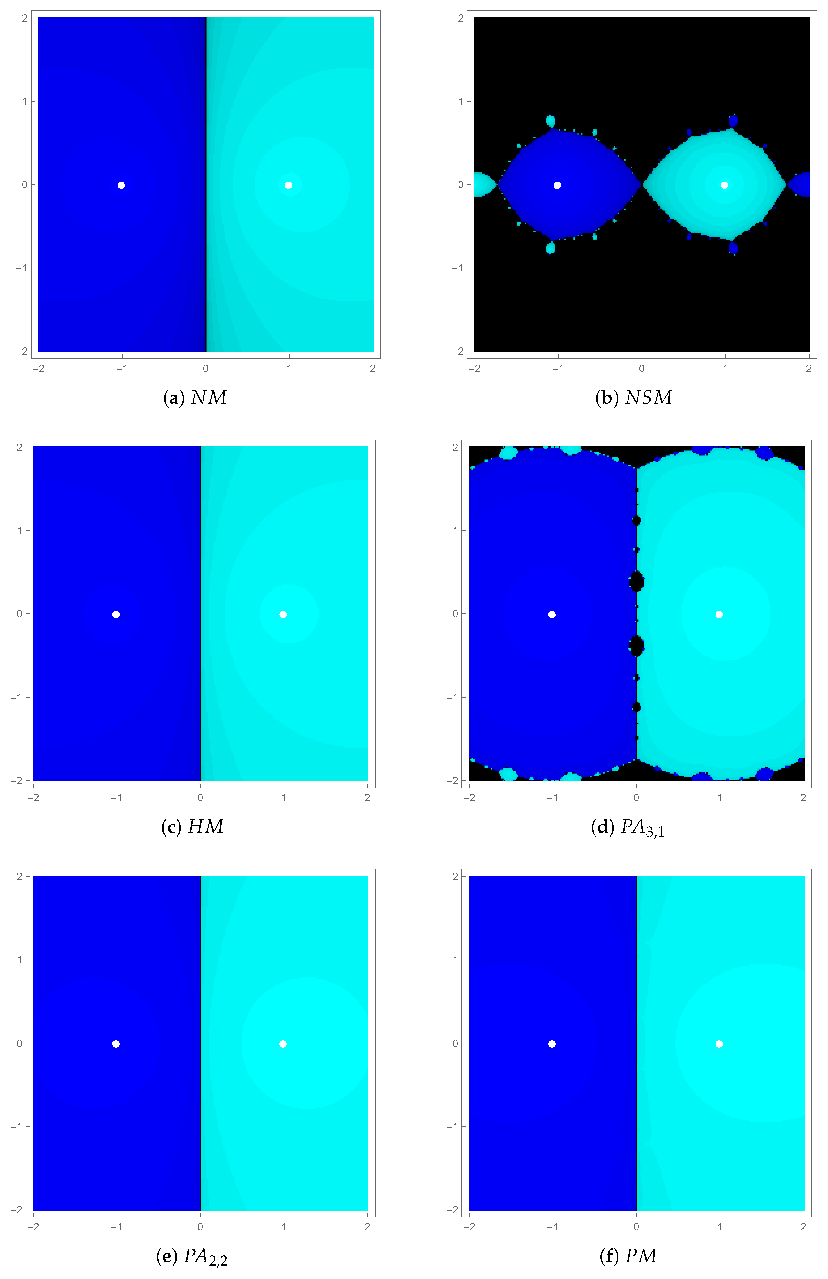
We consider a region . The region has grid size of and has two simple roots and 1. The convergence was determined by the stopping criteria . The exact location of roots is shown by two white dots within the basins. The dark blue color (left side of basins) represent the convergence region corresponding to the root and the light blue color (right side of basins) represent the convergence region corresponding to the root .
Figure 1 illustrates the basins for
(
5),
(
11),
(
12),
(
10), and the proposed method
(
18). It is evident from
Figure 1b,d that methods
and
exhibit local convergence, while the other methods exhibit the global convergence. Moreover,
Figure 1e,f illustarte broader and lighter basins of attraction because of higher convergence order of
and
as compared to the basins of
and
as shown in
Figure 1a,c. One can notice the symmetry in convergence region of each method. The convergence regions are symmetric about imaginary axis.
After achieving global convergence of the proposed method, it is important to examine certain critical factors related to matrix iterations, including convergence rate and numerical stability.
3.1. Convergence Analysis
Theorem 1. Suppose that the initial matrix has no eigenvalue on the imaginary axis, then the sequence of matrices generated from (18) converges to . Proof. Let
be Jordan decomposition of matrix
and consider
where
R is the rational function linked to (
18). Consequently, this will lead to the mapping of an eigenvalue
of
to an eigenvalue
of
. Also,
R will satisfy the properties given as follows:
∀.
with converges to , where .
To achieve this objective, consider
as the Jordan decomposition of
A that can be modified as [
2]
where
P is a non singular matrix while Jordan blocks
C and
N are associated to the eigenvalues in
and
respectively. Let the principal diagonals of blocks
C and
N have values
and
respectively. Then
Now, define a sequence
with
. Then from (
18), we get
Mathematical induction states that all ’s for will be diagonal if is diagonal. When is not diagonal, the proof may be considered in the similar methodology as stated at the end of the proof.
Now, (
25) can be written for scalar case
as follows:
where
and
. Furthermore,
, with
and therefore from (
26),
The factor
is bounded for
and does not affect the convergence. Furthermore, by selecting the right initial matrix
and
, we get
implying that
and hence
.
In the case when
is not a diagonal matrix, it is essential that we investigate the relation between the eigenvalues of
’s which was briefly explained at the starting of the proof.
In a comparable approach, it is clear from (
29) that
’s will converge to
, i.e.,
As a result, it is easy to conclude that
which finishes the proof. □
Theorem 2. Considering the assumptions of Theorem 1, the matrix sequence generated from (18) has convergence rate five to . Proof. Since,
depends on matrix
A∀
and the matrix
A commutes with
S, so
also commutes with
S∀
. Taking into consideration the substitution
we get,
Apply any type of matrix norm to the both sides of (
33),
This completes the proof. □
3.2. Stability Issues
Theorem 3. Considering the assumptions of Theorem 1, the sequence of matrix iterations generated from (18) is stable asymptotically. Proof. The iterate obtained from (
18) is a function of
A because of
, and hence commutes with
A. Let
be the perturbation generated at
iterate in (
18). Then
Based on the results of the error analysis of order one, we may consider that
,
. As long as
is small enough, this usual adjustment will work. Also suppose that
for larger
l, then we get
Here, the identity [
18] given by
has been applied, where
B is any nonsingular matrix and
C is any matrix. Also, considering
, we get
At this point, it is possible to deduce that
is bounded, i.e.,
which completes the proof. □
4. Extension to Determine Generalized Eigenvalues of a Matrix Pencil
Let
. Then
is said to be a generalized eigenvalue of a matrix pencil
if there exists a non-zero vector
such that
Here
will be a generalized eigenvector corresponding to
and (
40) is referred as a generalized eigenvalue problem. This can be determined by finding the zeros of characteristic polynomial
.
Complex problem solving in physics was the first scenario for the appearance of the characteristic polynomial and the eigenproblem. For a recent coverage of the topic one can see [
19]. When more generality is needed, generalized eigenvalue problem is taking the place of the classical approach [
20].
Problem (
40) arises in several fields of numerical linear algebra. However, the dimensions of matrices
A and
B are typically quite enormous, hence further complicating the situation. There are a lot of different approaches that claim to be able to solve (
40) including the necessary eigenvectors in a smaller subspace or series of matrix pencils [
21,
22,
23] or using matrix decomposition [
24,
25,
26]. Our interest is in employing the matrix sign function which involves evaluating certain matrix sign computations based on the given matrix pencil to compute the required decomposition and hence to solve the problem (
40).
To solve the problem (
40) for the case of regular matrix pencils using matrix sign function, we consider rank revealing
decomposition [
27] after computing sign of two matrices depending on the given matrix pencil.
Theorem 4. Let such that be a regular matrix pencil and let and are defined aswhere and are sign functions given by If and are decompositions of and such that and are upper triangular, thenwhere ’s are eigenvalues of , and are the diagonal entries of and respectively for . Moreover, if B is non-invertible, then for some i which implies that some eigenvalues of will be infinity. Let
denotes tolerance value and
be the maximum iterations. Then, in accordance with the proposed method (
18) and Theorem 4, we propose Algorithm 1 to find out the eigenvalues of a regular matrix pencil
.
| Algorithm 1 Evaluating generalized eigenvalues of |
Require:
Ensure:
- 1:
Initialize . - 2:
while and do - 3:
- 4:
return . - 5:
end while - 6:
Construct decomposition of as follows: . - 7:
Initialize . - 8:
Repeat step 2–5 to return . - 9:
Construct decomposition of as follows: . - 10:
Compute two matrices and , where . - 11:
if ∀ then - 12:
for i=1:n do - 13:
. - 14:
end for - 15:
end if
|
6. Numerical Aspects
In this section, we have examined a variety of examples to evaluate our proposed method by comparing it with various existing techniques. For this study, we have assumed the following stopping criteria:
where
stands for the tolerance value and
will be suitable matrix norm. Also,
and
norms are considered for real and complex input matrices, respectively [
14].
For the sake of comparison, we only consider the methods that exhibit global convergence and we do not include any methods that have local convergence. The methods that are being compared will be
(
5),
(
6),
(
12),
((
10) for
),
(
13),
(
18) and
(
20) with spectral scaling (
19). All simulations are done in Mathematica using system specifications “Windows 11 Home Intel(R) Core(TM) i7-1255U CPU running at 1.70 GHz processor having 16.0 RAM (64-bit operating system)”.
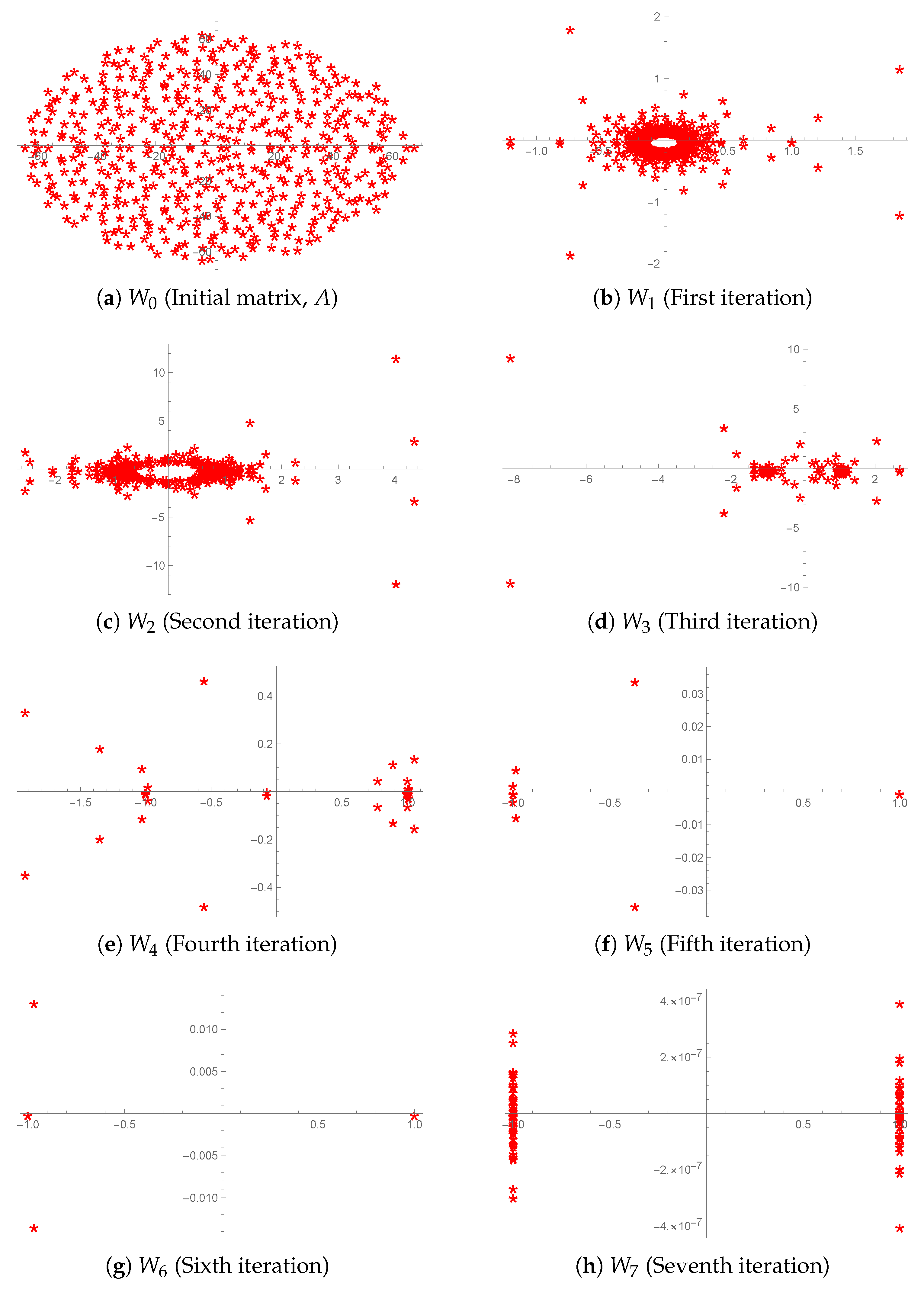
Example 1. Here, we perform the eigenvalue clustering of a random real matrix given as
SeedRandom[100]; A = RandomReal[{-5,5},{500,500}];
The outcomes are shown in
Figure 3 using the stopping criteria (
45) with
norm and
. We can see that eigenvalues of
are scattered at the initial stage as shown in
Figure 3a, while proceeding for the next iterations
in
Figure 3b–g for
respectively using
(
18), the eigenvalues are converging towards 1 or
. Then in
Figure 3h, all eigenvalues converge to 1 or
(based on the stopping criteria) implying that the sequence of matrices
converges to
. The result of Theorem 1 is therefore confirmed.
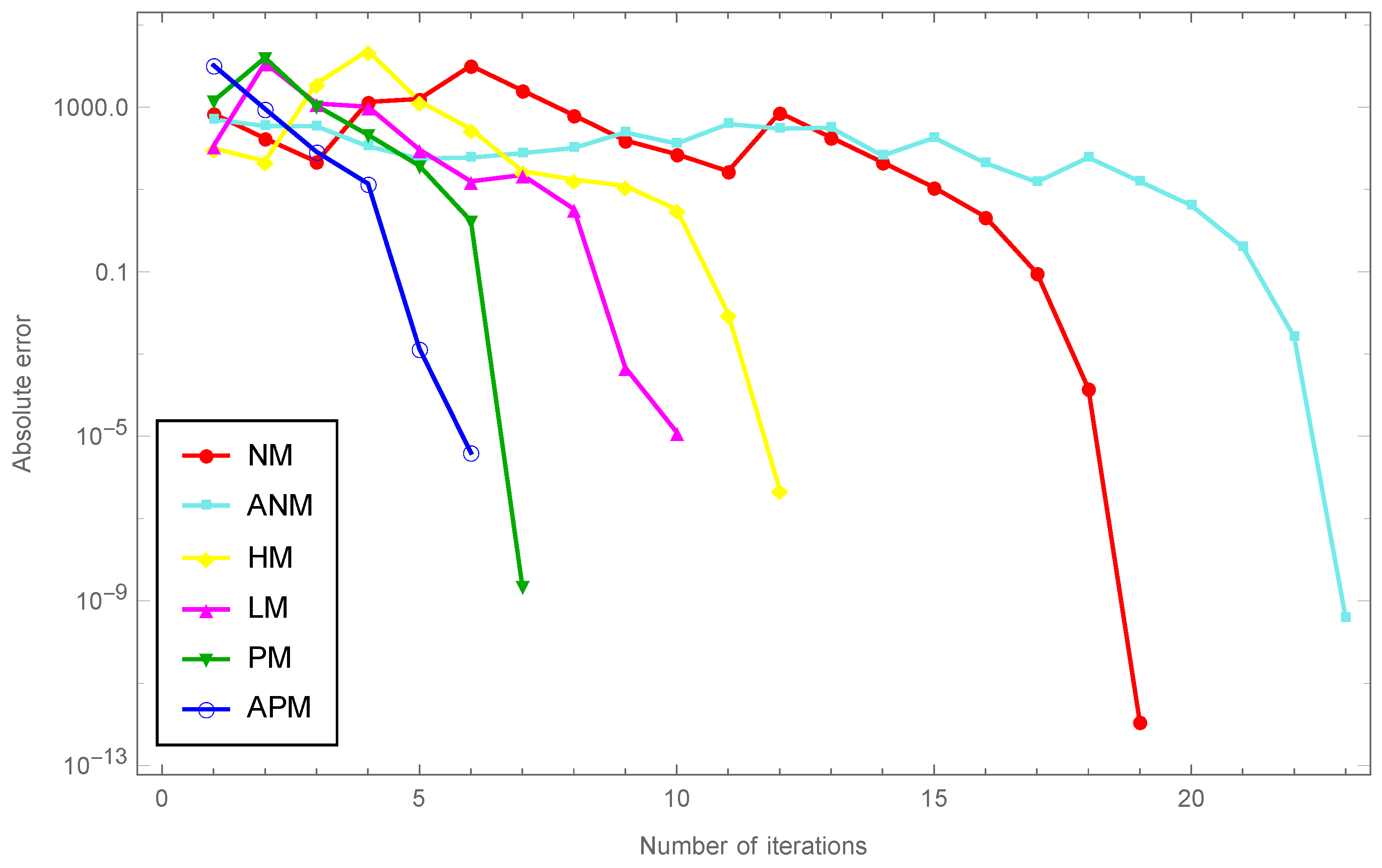
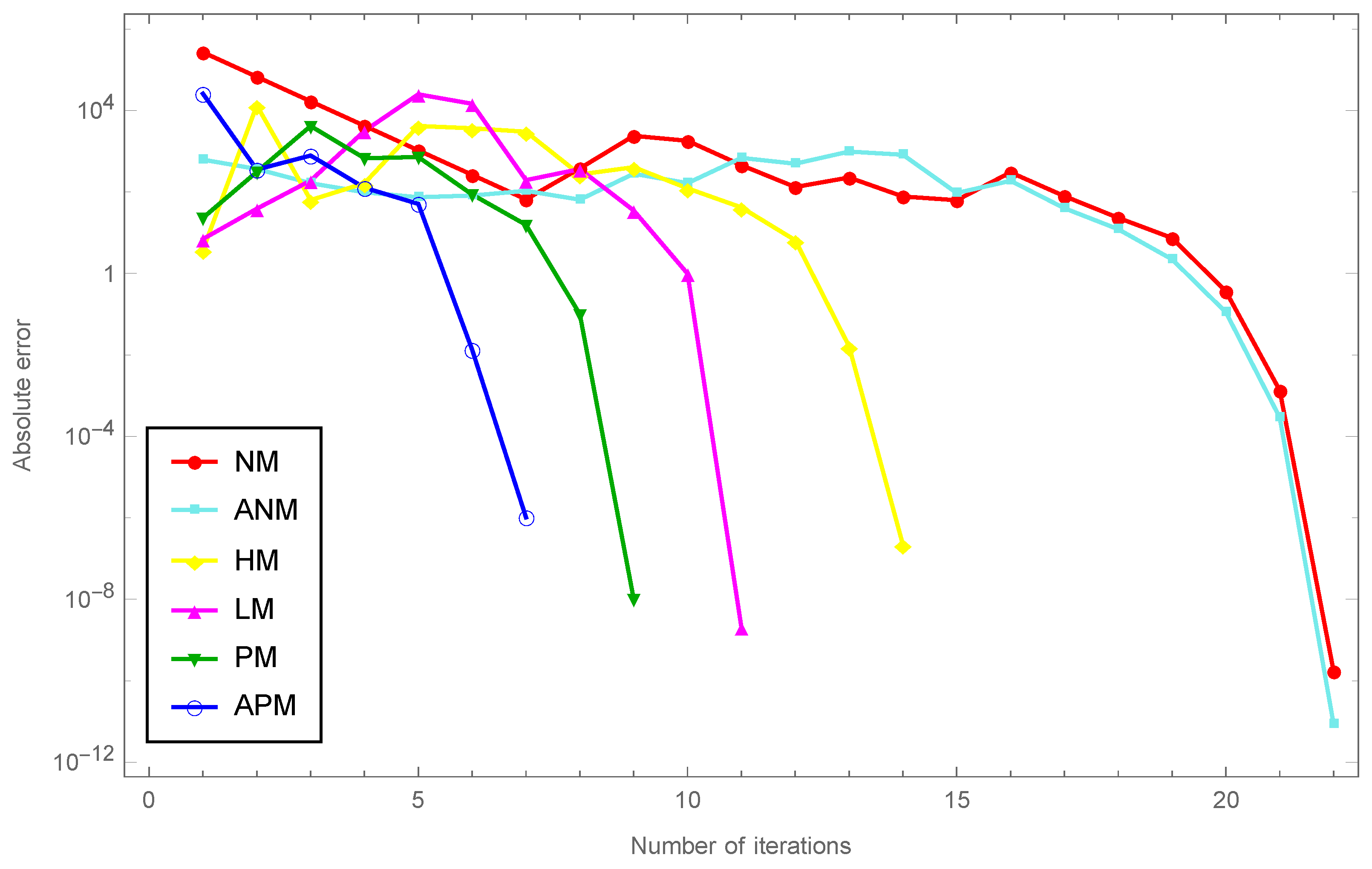
Example 2. In this example, convergence of many different methods for computing has been compared, where A is a random complex square matrix given as follows:
SeedRandom[101];
A = RandomComplex[{-1 - 1.5 I, 1 + 1.5 I}, {1000, 1000}]
The comparison is shown in
Figure 4 with
and
norm which illustrates the results with regard to the number of iterations and the absolute error and demonstrates the consistent behavior of both
and
.
Example 3. This example presents a comparison on convergence of many different methods for computing , where A is a random real square matrix given as
SeedRandom[111];
A = RandomReal[{-25, 25}, {2000, 2000}];
The comparison is presented in
Figure 5 with
and
norm which illustrates the results with respect to the number of iterations and the absolute error and demonstrates the consistent behavior of both
and
for evaluating
.
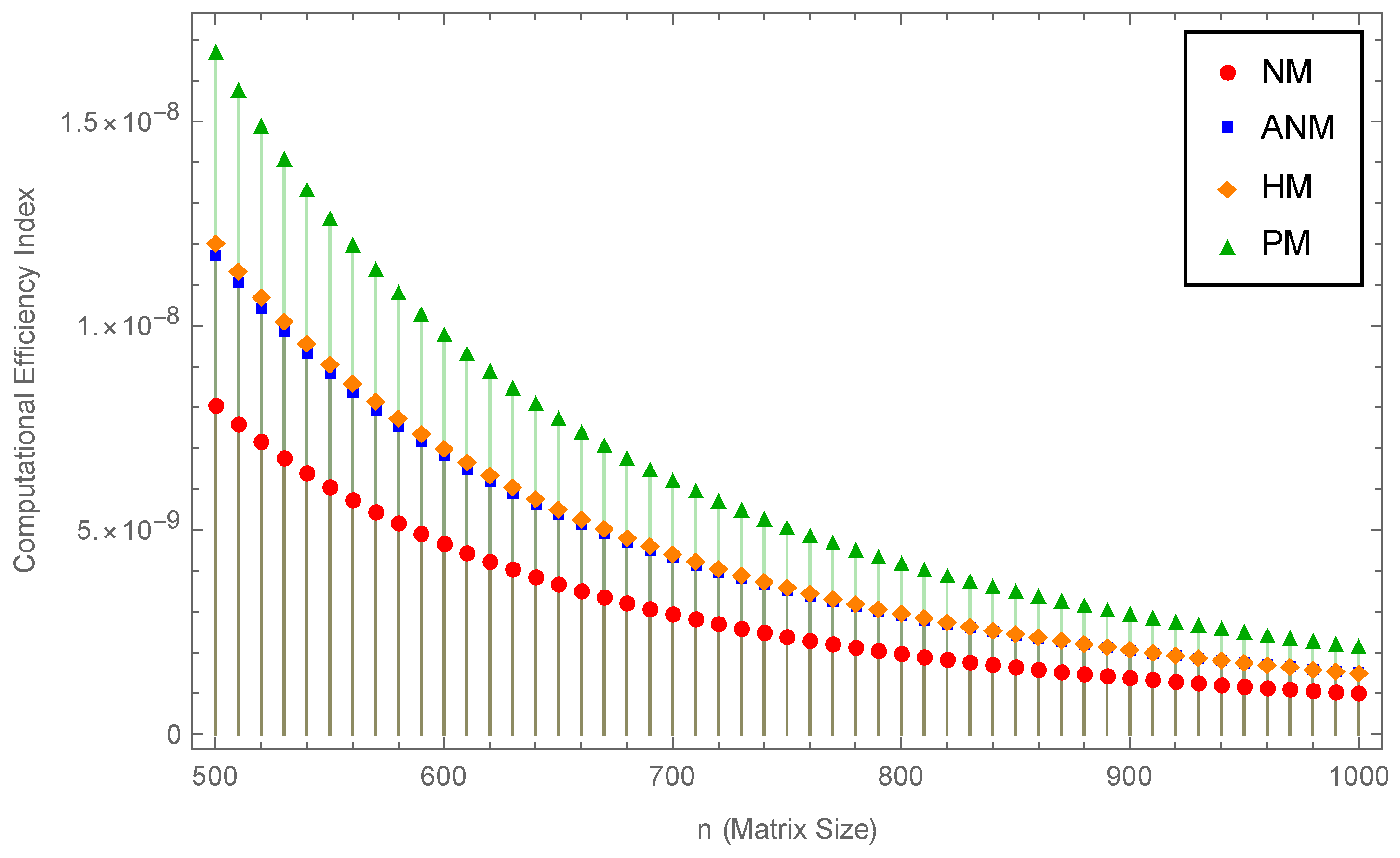
Example 4. Here, we examine the convergence of various methods with regard to the iteration number and the timings of CPU for evaluating the sign function of ten random matrices:
SeedRandom[121]; number = 10; tolerance = 10^(-5);
Table[A[j] = RandomComplex[{-3 - 2 I, 3 + 2 I}, {50j, 50j}];, {j, number}];
The comparative analysis based on iteration number and CPU timings for matrices of various sizes, are presented in
Table 2 and
Table 3 respectively using
and
-norm. The implementation of new methods
and
result in an improvement in the average iteration number and the amount of time spent by CPU. The outcomes demonstrate that the suggested method
is significantly better as compared to other fifth order methods like
and
.
Now, in Examples 5 and 6, we aim to evaluate generalized eigenvalues of matrix pencils using matrix sign function for which we use Algorithm 1 for different methods by replacing (
18) with existing methods in Step 3.
Example 5. Let be a matrix pencil, where matrices A and B are given by [30]where is the identity matrix of size 20. The eigenvalues of given pencil
are
for
and remaining eigenvalues are infinite. We verify these eigenvalues using proposed method and Algorithm 1. We compute the matrices
and
and then calculate
from Algorithm 1. The outcomes are presented in
Table 4 for
.
Moreover, for which implies that for . Hence this example verifies the results given in Theorem 4.
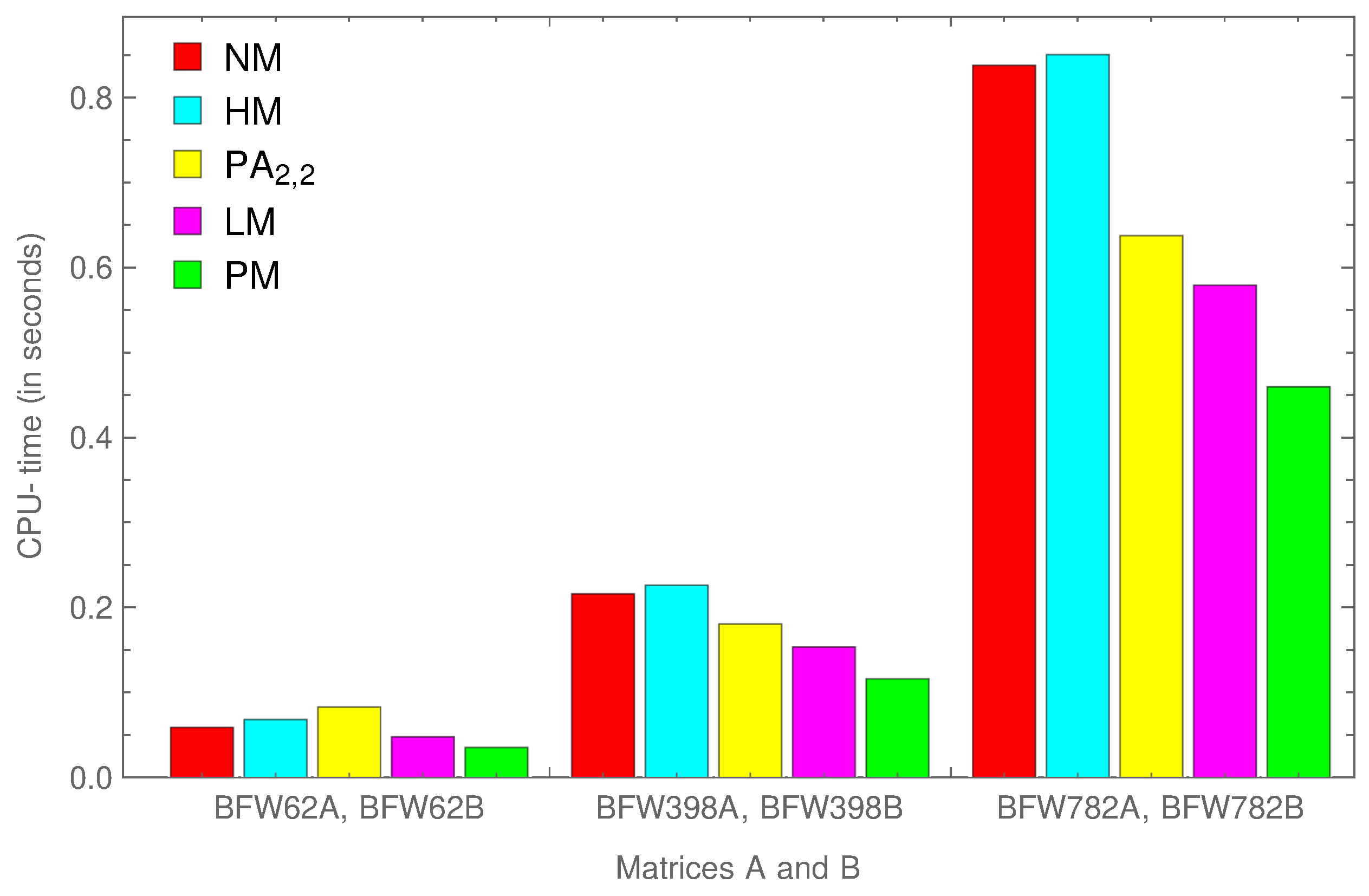
Example 6 (Bounded finline dielectric waveguide problem)
. The generalized eigenvalue problem (40) arises in the finite element analysis for finding the propagating modes of a rectangular waveguide. We consider three cases for the pairs of matrices A and B as ; and from the Matrix Market [31]. Table 5 shows the outcomes depending on the iteration numbers
and
for computing
and
with corresponding absolute errors
and
using stopping criterion (
45) with
. Also, total computational time in seconds taken for computing
and
has been compared in
Figure 6. The outcomes demonstrate that the suggested method is better with respect to errors and timings.


