On a Fifth-Order Method for Multiple Roots of Nonlinear Equations

Abstract

There are several measures for comparing methods for solving a single nonlinear equation. The first is the order of convergence, then the cost to achieve such rate. This cost is measured by counting the number of functions (and derivatives) evaluated at each step. After that, efficiency is defined as a function of the order of convergence and cost. Lately, the idea of basin of attraction is used. This shows how far one can start and still converge to the root. It also shows the symmetry/asymmetry of the method. It was shown that even methods that show symmetry when solving polynomial equations are not so when solving nonpolynomial ones. We will see here that the Euler–Cauchy method (a member of the Laguerre family of methods for multiple roots) is best in the sense that the boundaries of the basins have no lobes. The symmetry in solving a polynomial equation having two roots at $\pm 1$ with any multiplicity is obvious. In fact, the Euler–Cauchy method converges very fast in this case. We compare one member of a family of fifth-order methods for multiple roots with several well-known lower-order and efficient methods. We will show using a basin of attraction that the fifth-order method cannot compete with most of those lower-order methods.

1. Introduction

The solution of a single nonlinear equation

$$f\left(x\right)=0$$

(1)

can be found in applied science and engineering; see some examples in [1,2]. Here, we are interested in the case that the function $f\left(x\right)$ has roots of multiplicity $m\ge 2.$ These methods are based either on the knowledge of the multiplicity or on methods for simple roots for the function $g\left(x\right)=f\left(x\right)/f^{\prime }\left(x\right)$; see Traub [3] and the more recent book by Petković et al. [4]. Neta [5] and Herceg and Petković [6] discussed the extension of Popovski’s method [7] to the case of multiple roots using these two ideas. Several well-known methods for multiple roots of order two and higher can be found in the literature. Recently, a new family of fifth order was suggested by Thangkhenpau et al. [8]. The method is

$$\begin{array}{c}{\displaystyle y_n=x_n-m\frac{f\left(x_n\right)}{f^{\prime }\left(x_n\right)+\alpha f\left(x_n\right)}}\hfill \\ \\ {\displaystyle x_{n+1}=y_n-mW\left(t_n\right)\frac{f\left(y_n\right)}{f^{\prime }\left(y_n\right)+\alpha f\left(y_n\right)}}\hfill \end{array}$$

(2)

where $t_n={\left(\frac{f^{\prime }\left(y_n\right)}{f^{\prime }\left(x_n\right)}\right)}^{\frac{1}{m-1}}$, $\alpha$ is a small real parameter, and W is a weight function. The authors prove that, under certain conditions on the weight function, the method is of order five and requires four function evaluations per cycle. Several weight functions were suggested. The order of a method is p if

$$|x_{n+1}-\xi |\le C_p{|x_n-\xi |}^p$$

(3)

where $\xi$ is the root. Given a method of order p requiring d function and derivative evaluation per cycle, we define the efficiency index $E_I$ (see, e.g., [4]):

$$E_I=p^{1/d}.$$

(4)

In this paper, we compare the performance of (2) with the second-order method (see Schröder [9] or Rall [10])

$$x_{n+1}=x_n-m\frac{f\left(x_n\right)}{f^{\prime }\left(x_n\right)}$$

(5)

and with third-order methods due to Euler–Cauchy [11] and Dong [12].

The Euler–Cauchy method is a special case of Laguerre’s method for multiple roots (see Bodewig [11] and Neta and Chun [13]):

$${\displaystyle x_{n+1}=x_n-\frac{2m\frac{f\left(x_n\right)}{f^{\prime }\left(x_n\right)}}{1+\sqrt{(2m-1)-2m\frac{f\left(x_n\right)f^{\prime \prime }\left(x_n\right)}{f^{\prime }{\left(x_n\right)}^2}}}.}$$

(6)

In [14], Dong introduced two methods that did not perform as well as the two methods in his later paper [12]. These latter ones, called here Dong3 and Dong4, are given by

$$\begin{array}{ccc}{\displaystyle y_n}\hfill & =& {\displaystyle x_n-\frac{f\left(x_n\right)}{f^{\prime }\left(x_n\right)},}\hfill \\ {\displaystyle x_{n+1}}\hfill & =& {\displaystyle y_n-\frac{f\left(x_n\right)}{{\displaystyle {\left({\displaystyle \frac{m}{m-1}}\right)}^{m+1}{f}^{\prime }\left(y_n\right)+\frac{m-m^2-1}{{\left(m-1\right)}^2}{f}^{\prime }\left(x_n\right)}},}\hfill \end{array}$$

(7)

and

$$\begin{array}{ccc}{\displaystyle y_n}\hfill & =& {\displaystyle x_n-\frac{m}{m+1}\frac{f\left(x_n\right)}{f^{\prime }\left(x_n\right)},}\hfill \\ \\ {\displaystyle x_{n+1}}\hfill & =& {\displaystyle y_n-\frac{{\displaystyle \frac{m}{m+1}f\left(x_n\right)}}{{\displaystyle {\left(1+\frac{1}{m}\right)}^m{f}^{\prime }\left(y_n\right)-f^{\prime }\left(x_n\right)}}.}\hfill \end{array}$$

(8)

Clearly, method (2) has an efficiency index of $5^{1/4}=1.4953$, which is better than the third-order method above, whose index is $3^{1/3}=1.4422$, and Schröder’s method, whose index is $2^{1/2}=1.4142$.

The reason for choosing these methods for the comparison is that they were shown to be superior to other methods of the same order; see [15,16,17]. The comparison is based on the idea of basins of attraction. The idea of basin of attraction was introduced by Stewart [18] and followed by the work of Amat et al. [17,19] and references there.

2. Basins of Attraction

Let R be a rational map on the Riemann sphere, and let $z_0$ be a periodic point of period ℓ, i.e., R^ℓ$\left(z_0\right)=z_0,$ where ℓ is the smallest such integer. If ℓ = 1, then $z_0$ is called a fixed point of the rational map R. For example, the rational map associated with Schröder’s method is given by

$$R\left(z\right)=z-m\frac{f\left(z\right)}{f^{\prime }\left(z\right)}.$$

The point $z_0$ is called neutral, attractive, or repelling based on $|R^{\prime }\left(z_0\right)|$ equal to, smaller, or larger than 1, respectively. Let R be the rational function associated with an iterative method to find multiple roots of f; then the fixed points of R that are not roots of f are called extraneous fixed points. The Julia set of a nonlinear map $R\left(z\right)$ is the closure of the set of its repelling periodic points. The complementary set in the Riemann sphere is the Fatou set; see [19,20].

Definition of basin of attraction. If a fixed point $\pi$ of R is attracting, then all nearby points of $\pi$ are attracted toward $\pi$ under the action of R; i.e., the iterates under R converge to $\pi .$ The collection of all points whose iterates under R converge to $\pi$ is called the basin of attraction of $\pi$.

3. Numerical Experiments

We compare (2) with $\alpha =0.1$ and the weight function

$$W\left(t\right)=\frac{1}{1-t^2}$$

(9)

on the following 5 nonlinear functions having various multiplicities:

• $f_1\left(z\right)={(z^2-1)}^2$
• $f_2\left(z\right)={(z^3-1)}^2$
• $f_3\left(z\right)={(z^3-z)}^4$
• $f_4\left(z\right)={(z^5-1)}^4$
• $f_5\left(z\right)={(z^2+1/4)}^3{\left(e^{z-1}-1\right)}^3.$

The comparison is performed on a 6 by 6 square centered at the origin and containing all the roots of the functions. We take a uniformly distributed set of points in the complex plane $z_{jk}=x_j+I{y}_k$, where $I=\sqrt{-1}$, $x_j=-3+(j-1)\Delta x,j=1,2,\dots N$ and $y_k=-3+(k-1)\Delta y,k=1,2,\dots M$. We took $\Delta x=\Delta y=0.01$ and $N=M=601$. Each of these points is used as a starting point for the iteration. We have collected the following data:

• Number of iterations required to converge within ${10}^{-7}$ (up to 40 iterations). Note that since the methods use a different number of function and derivative evaluations per iteration, we listed the number of function evaluations per iteration step.
• Which root the iteration converged to.
• CPU run time for the whole set of initial points. The computations are performed on a MacBook Pro 3.1 GHz Quad-Core Intel Core i7.
• The total number of points for which the iterative method did not converge.

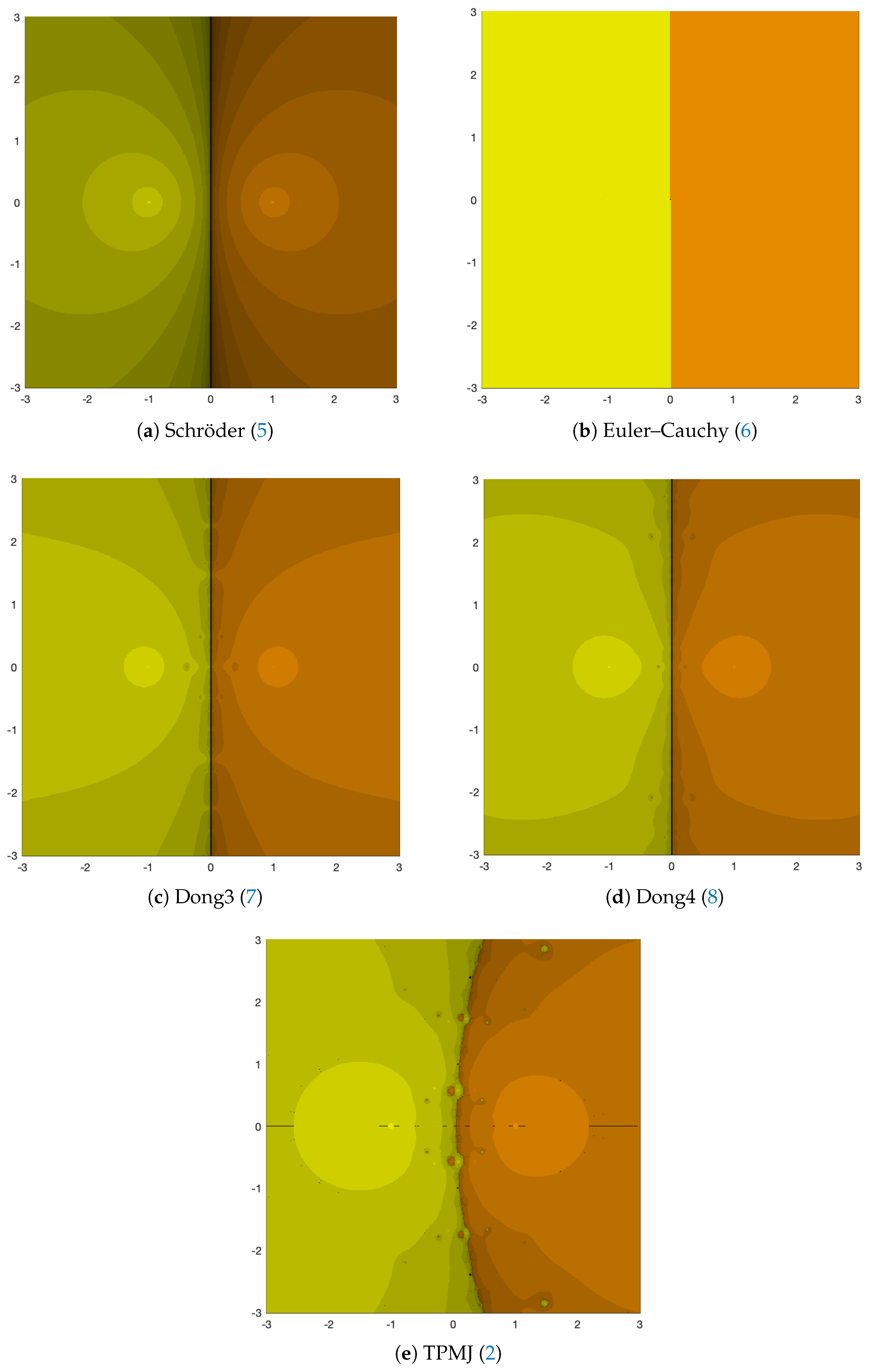
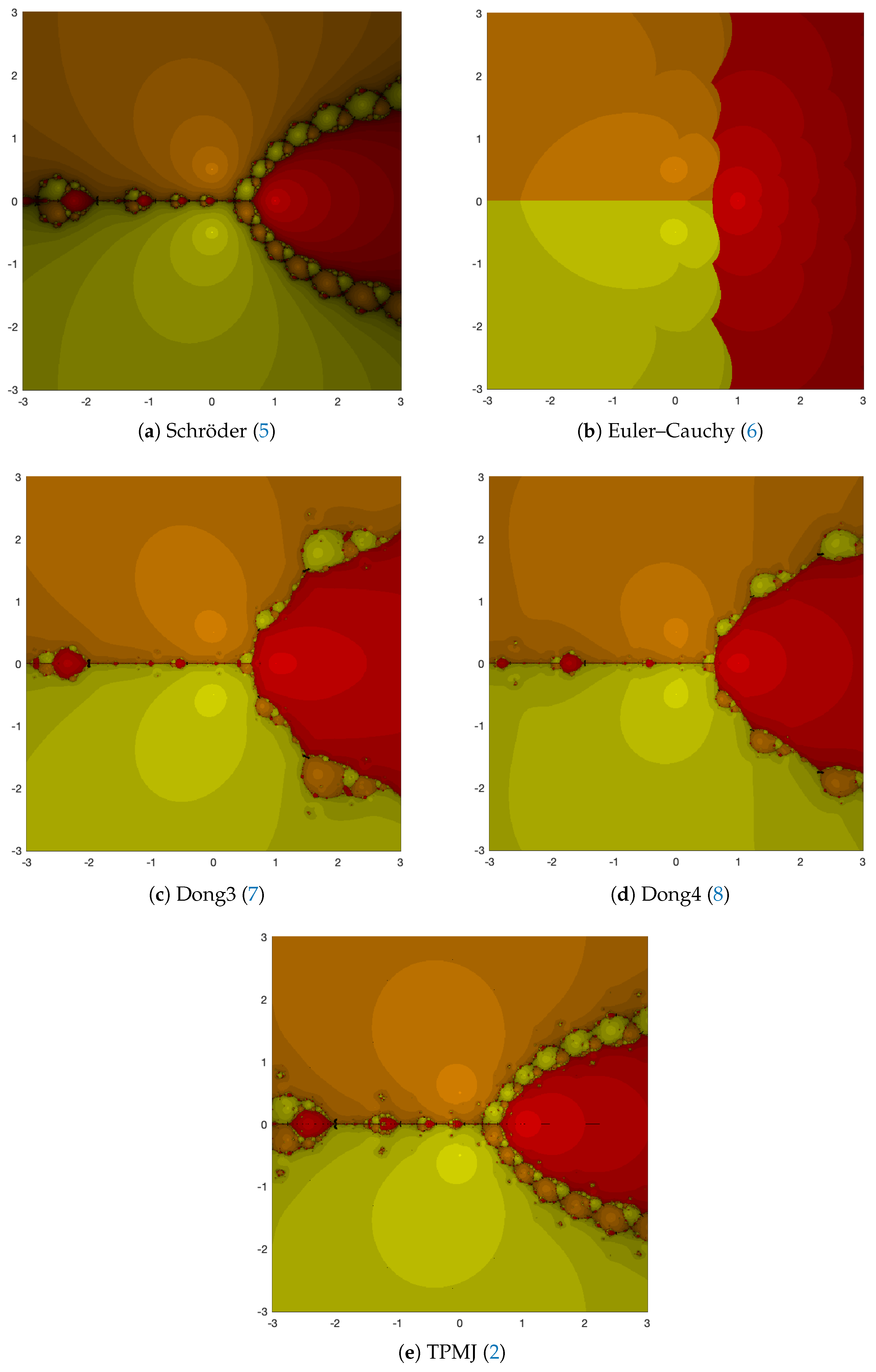
Each point is colored based on the root it converged to and black in case of divergence. In Figure 1, we plotted the basins of attraction for the 5 methods running on the first example.

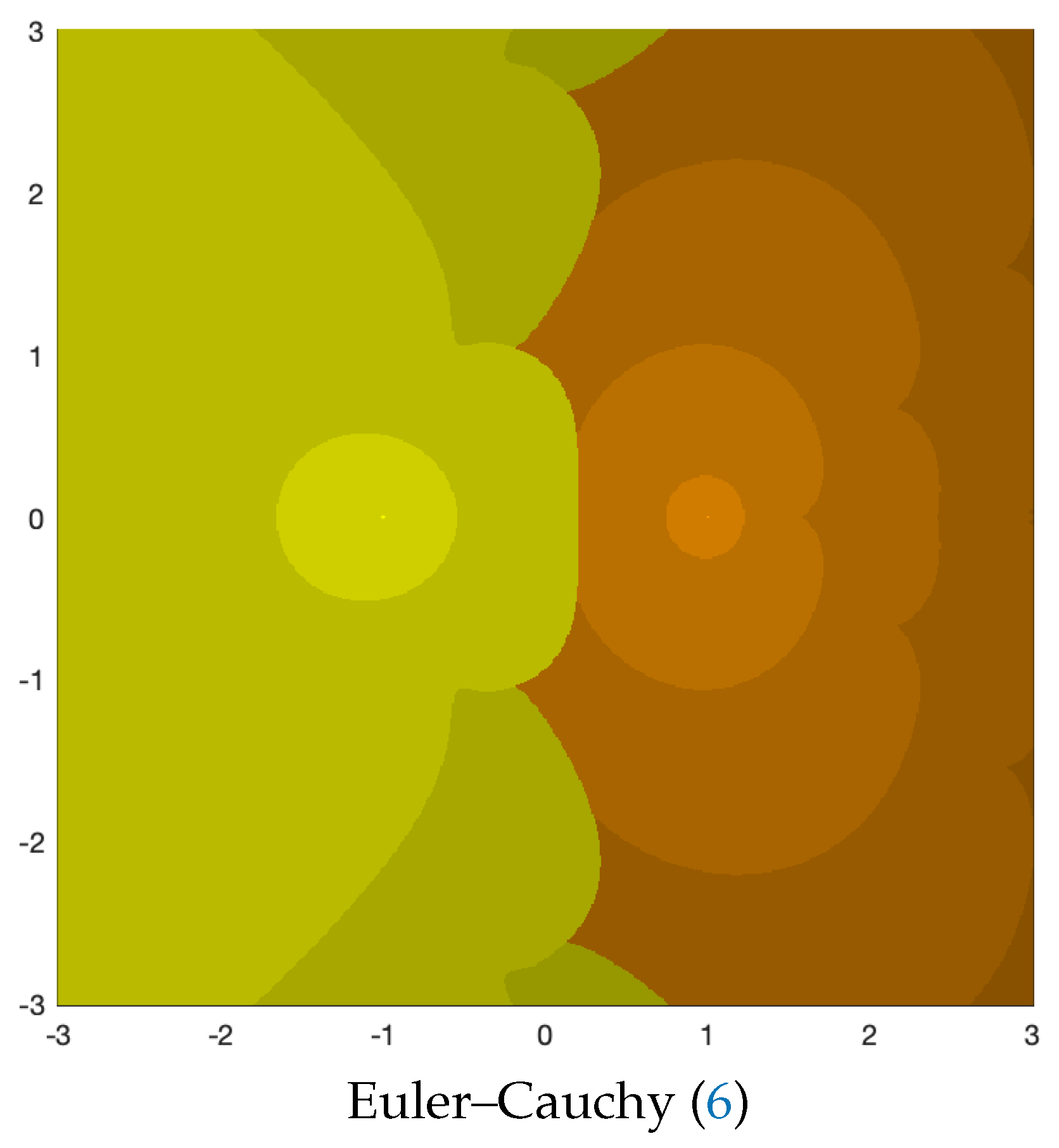
It is clear from the figure that the Euler–Cauchy method is best. There are no lobes along the boundary of the basins. Notice that the square domain is divided equally between the two basins. This symmetry does not show up when we find the double roots of the nonpolynomial

$$F\left(z\right)={(z+1)}^2{\left(e^{z-1}-1\right)}^2$$

as can be seen in Figure 2. Here, the boundary is no longer a vertical line through the origin. This asymmetry is also visible in Figure 1 for TPMJ.

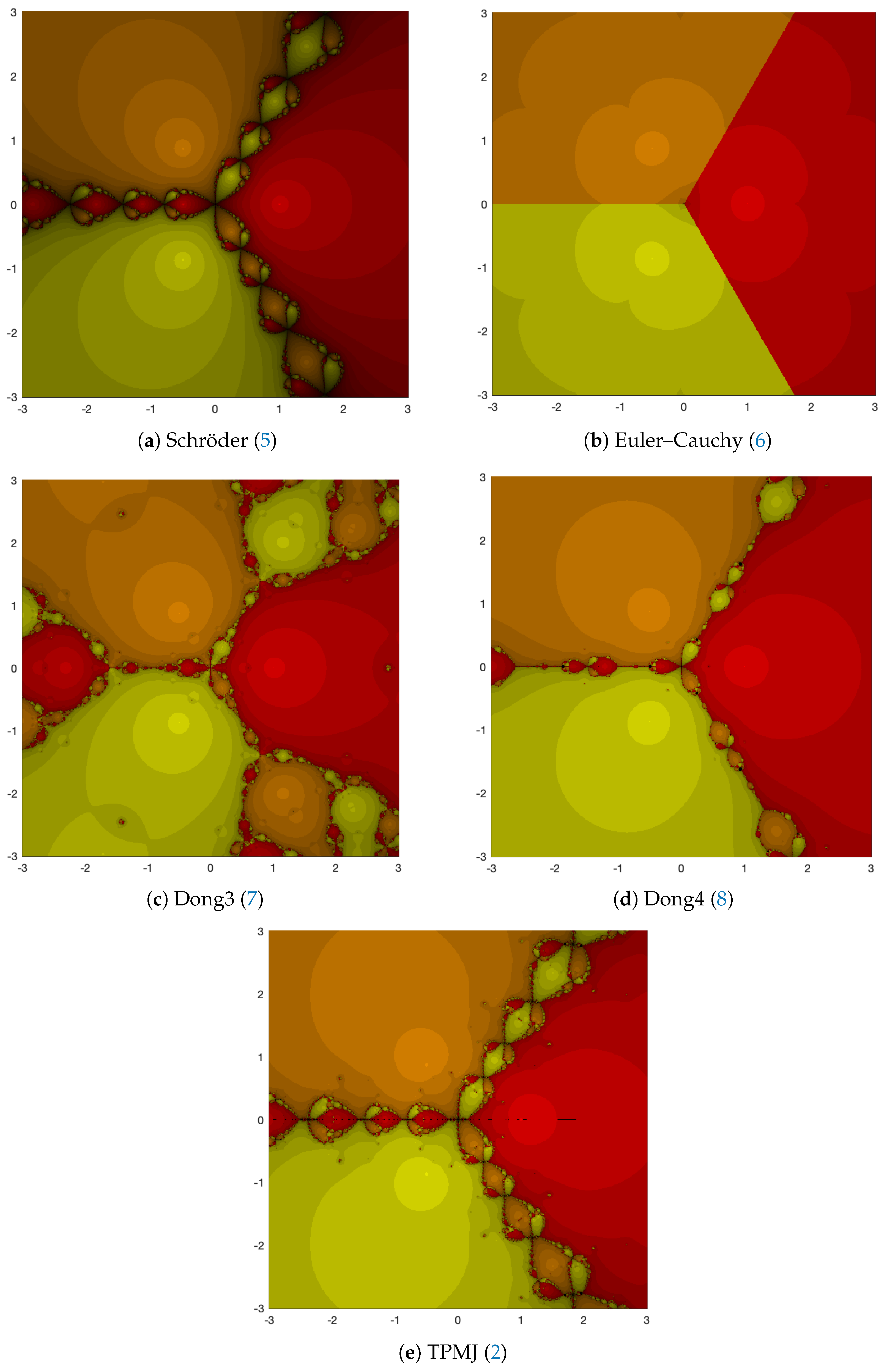
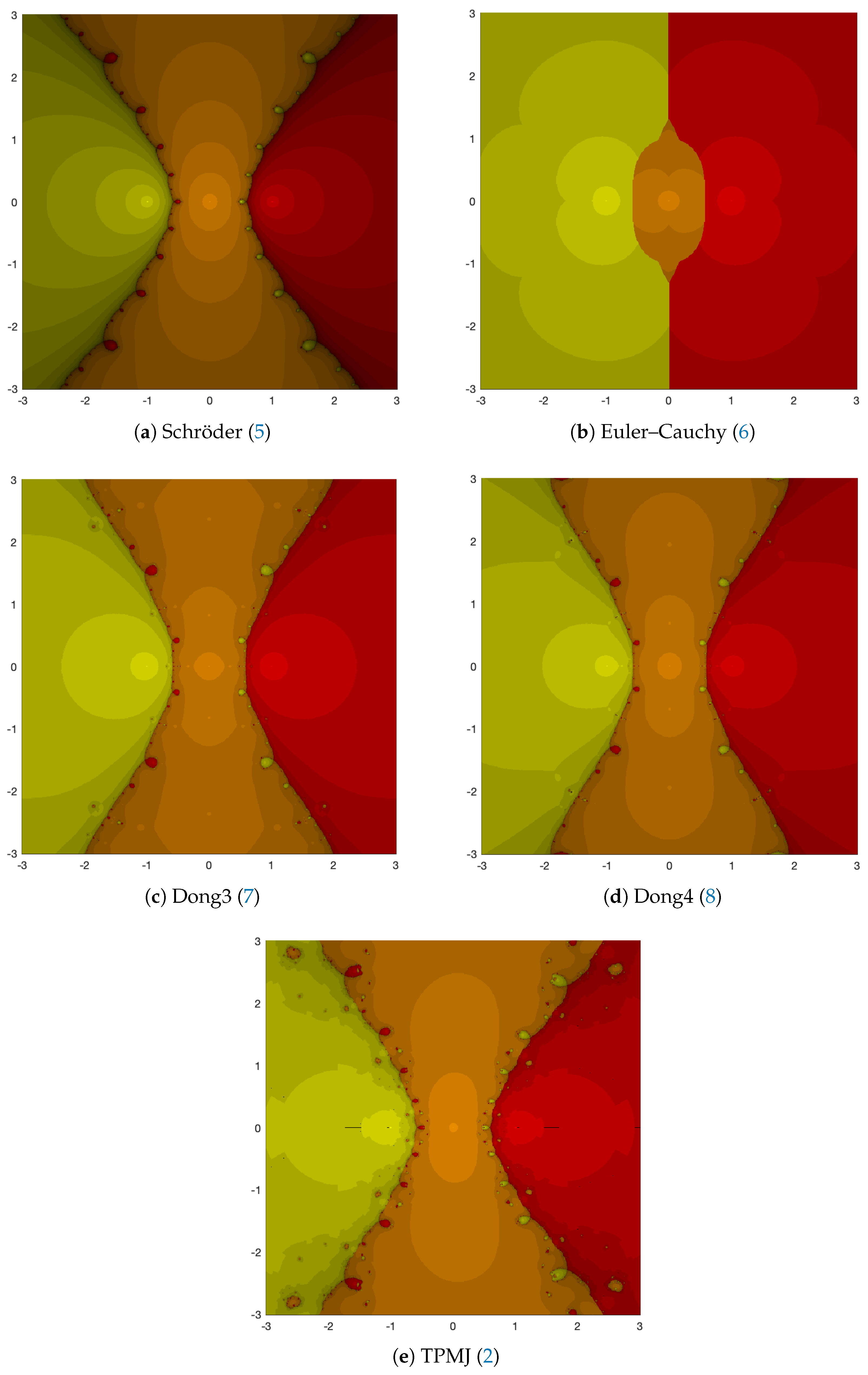
The symmetry of Euler–Cauchy shows also in the other examples except the fourth; see Figure 3, Figure 4, Figure 5 and Figure 6. Notice that in Figure 4, the basin for the root $z=0$ is much smaller for Euler–Cauchy than for the other schemes. In Figure 5, Euler–Cauchy has some bunny ears around the origin.

We now turn to more quantitative measures by listing the CPU run time (see

Table 1. CPU time (msec) for each example (1–5) and each of the methods.

Method	${\mathit{f}}_1$	${\mathit{f}}_2$	${\mathit{f}}_3$	${\mathit{f}}_4$	${\mathit{f}}_5$	Average
Schröder (5)	147.015	273.376	315.397	624.16	625.352	331.661
Euler–Cauchy (6)	103.597	488.069	601.789	939.69	1033.156	550.839
Dong3 (7)	173.106	331.946	373.455	488.017	671.488	332.285
Dong4 (8)	168.588	288.231	401.532	541.621	704.872	365.219
TPMJ (2)	232.999	419.495	1220.686	1870.103	1107.163	1233.198

), the average number of function evaluations per point (see

Table 2. Average number of function evaluations per point for each example (1–5) and each of the methods.

Method	${\mathit{f}}_1$	${\mathit{f}}_2$	${\mathit{f}}_3$	${\mathit{f}}_4$	${\mathit{f}}_5$	Average
Schröder (5)	11.65	15.21	14.62	22.22	16.31	16.00
Euler–Cauchy (6)	3.00	11.43	12.44	16.83	13.40	11.42
Dong3 (7)	11.10	15.08	12.84	13.78	12.77	13.12
Dong4 (8)	10.27	11.77	13.50	15.18	13.24	12.79
TPMJ (2)	13.04	16.84	16.32	23.72	17.46	17.47

), and the total number of divergent points (see

Table 3. Number of black points for each example (1–5) and each of the methods.

Method	${\mathit{f}}_1$	${\mathit{f}}_2$	${\mathit{f}}_3$	${\mathit{f}}_4$	${\mathit{f}}_5$	Average
Schröder (5)	601	8	0	5162	386	1231.4
Euler–Cauchy (6)	1	1	0	1	0	0.6
Dong3 (7)	601	1	0	8	177	157.4
Dong4 (8)	603	139	12	950	147	370.2
TPMJ (2)	248	354	94	222	457	275

).

It is clear from Table 1 that Euler–Cauchy is fastest, followed by Schröder’s method. The fifth-order method is slowest for the first example. The other two tables show the superiority of Euler–Cauchy in terms of the number of divergent points and the average number of function evaluations per point. In fact, Euler–Cauchy has the lowest number of divergent points in all examples, followed by Dong3. Unfortunately, Euler–Cauchy requires more CPU run time than the other methods except TPMJ.

Considering the column of averages in Table 1, Table 2 and Table 3, we can say that Schröder’s and Dong3 are fastest, followed by Dong4. The average number of function evaluations is lowest for Euler–Cauchy and Dong4, followed by Dong3. The number of divergent points is lowest for Euler–Cauchy, followed by Dong3 and TPMJ.

4. Conclusions

Even though TPMJ (2) is of higher order and having a higher-efficiency index, it is the slowest method (about four times of any other scheme). It requires almost as many function evaluations per point as the second-order method. The number of divergent points is smaller than that for Schröder and Dong4. The symmetry observed in the basins of all methods for example 1 does not manifest itself in the case of TPMJ for which the basin for the root $z=-1$ is larger (Figure 1). The basins for Dong3 for example 2 are more chaotic than for the others.

References

- Sharma, J.R.; Kumar, D.; Cattani, C. An efficient class of weighted-Newton multiple root solvers with seventh order convergence. Symmetry 2019, 11, 1054. [Google Scholar] [CrossRef]
- Zafar, F.; Cordero, A.; Rizvi, D.E.Z.; Torregrosa, J.R. An optimal eighth order derivative free multiple root finding scheme and its dynamics. AIMS Math. 2023, 8, 8478–8503. [Google Scholar] [CrossRef]
- Traub, J.F. Iterative Methods for the Solution of Equations; Prentice Hall: New York, NY, USA, 1964. [Google Scholar]
- Petković, M.S.; Neta, B.; Petković, L.D.; Džunić, J. Multipoint Methods for the Solution of Nonlinear Equations; Elsevier: Amsterdam, The Netherlands, 2012. [Google Scholar]
- Neta, B. Basins of attraction for family of Popovski’s methods and their extension to multiple roots. J. Numer. Anal. Approx. Theory 2022, 51, 88–102. [Google Scholar] [CrossRef]
- Herceg, D.; Petković, I. Computer visualization and dynamic study of new families of root-solvers. J. Comput. Appl. Math. 2022, 401, 113775. [Google Scholar] [CrossRef]
- Popovski, D.B. A family of one point iteration formulae for finding roots. Int. J. Comput. Math. 1980, 8, 85–88. [Google Scholar] [CrossRef]
- Thangkhenpau, G.; Panday, S.; Mittal, S.K.; Jäntschi, L. Novel parametric families of with and without memory iterative methods for multiple roots of nonlinear equations. Mathematics 2023, 11, 2036. [Google Scholar] [CrossRef]
- Schröder, E. Über unendlich viele Algorithmen zur Auflösung der Gleichungen. Math. Ann. 1870, 2, 317–365. [Google Scholar] [CrossRef]
- Rall, L.B. Convergence of the Newton process to multiple solutions. Numer. Math. 1966, 9, 23–37. [Google Scholar] [CrossRef]
- Bodewig, E. Sur la méthode Laguerre pour l’approximation des racines de certaines équations algébriques et sur la critique d’Hermite. Indag. Math. 1946, 8, 570–580. [Google Scholar]
- Dong, C. A family of multipoint iterative functions for finding multiple roots of equations. Intern. J. Comput. Math. 1987, 12, 363–367. [Google Scholar] [CrossRef]
- Neta, B.; Chun, C. On a family of Laguerre methods to find multiple roots of nonlinear equations. Appl. Math. Comput. 2013, 219, 10987–11004. [Google Scholar] [CrossRef]
- Dong, C. A basic theorem of constructing an iterative formula of the higher order for computing multiple roots of an equation. Math. Numer. Sin. 1982, 11, 445–450. [Google Scholar]
- Chun, C.; Neta, B. Basins of attraction for several third order methods to find multiple roots of nonlinear equations. Appl. Math. Comput. 2015, 268, 129–137. [Google Scholar] [CrossRef]
- Amat, S.; Busquier, S.; Plaza, S. Dynamics of a family of third-order iterative methods that do not require using second derivatives. Appl. Math. Comput. 2004, 154, 735–746. [Google Scholar] [CrossRef]
- Chun, C.; Neta, B. Comparative study of methods of various orders for finding repeated roots of nonlinear equations. J. Comput. Appl. Math. 2018, 340, 11–42. [Google Scholar] [CrossRef]
- Stewart, B.D. Attractor Basins of Various Root-Finding Methods. Master’s Thesis, Naval Postgraduate School, Department of Applied Mathematics, Monterey, CA, USA, 2001. [Google Scholar]
- Amat, S.; Busquier, S.; Plaza, S. Review of some iterative root-finding methods from a dynamical point of view. Scientia 2004, 10, 3–35. [Google Scholar]
- Blanchard, P. Complex analytic dynamics on the Riemann sphere. Bull. Am. Math. Soc. 1984, 11, 85–141. [Google Scholar]
Figure 1.
Basins of attraction of analyzed methods for the roots of the function .
Figure 2.
Basins of attraction of the Euler–Cauchy method for the roots of the nonpolynomial .
Figure 3.
Figure 4.
Figure 5.
Figure 6.