Article

Distributed Rotational Inertia Load Excitation Model and Its Impact on High-Speed Jointed Rotor Dynamic Response

1
School of Energy and Power Engineering, Beihang University, Beijing 102206, China
2
Shenyang Engine Design and Research Institute, Aero Engine Corporation of China, Shenyang 110015, China
3
Research Institute of Aero-Engine, Beihang University, Beijing 102206, China
*
Author to whom correspondence should be addressed.
Symmetry 2023, 15(11), 2009; https://doi.org/10.3390/sym15112009
Submission received: 9 October 2023 / Revised: 28 October 2023 / Accepted: 30 October 2023 / Published: 1 November 2023
(This article belongs to the Special Issue Symmetry in Mechanical Engineering: Properties and Applications)

Abstract

:
Contemporary aero-engines aim for enhanced efficiency and weight reduction. They are designed to increase rotor operational speed while reducing rotor bending stiffness. This may result in bending deformation in rotor systems within the operational speed range. Such deformation can change the relative positions of rotor components, potentially causing increased mass asymmetry or unbalance. Traditional rotor dynamic models typically assume a constant rotor state. They approximate unbalance using constant mass eccentricities at certain rotor cross-sections. However, this approach has its limitations. This paper focuses on a high-speed jointed rotor system. A distributed rotational inertia load excitation model is proposed. This model explicitly considers the rotor’s variable unbalance state at different operational speeds. The study involves both simulations and experimental investigations. The results show that at high speeds, bending deformation causes the unbalance and rotational inertia load to shift from a concentrated to a distributed state. Notably, the localized rotational inertia moment from thin-disk components like turbine disks becomes significant at high speeds. This results in a rapid increase in bearing load with rotational speed. It also profoundly affects the rotor’s joints, causing interfacial slip and sudden changes in rotor vibration characteristics.

1. Introduction

As aero-engines continuously pursue performance improvement and structural efficiency, their structural systems confront progressively intricate dynamic challenges. Notably, the rotor systems of these aero-engines may cause vibrations that exceed acceptable limits if they exhibit poor unbalance states. This concern becomes particularly pronounced for jointed rotors, where joints may undergo deformation due to interfacial slip damage, resulting in alterations in the rotor’s unbalance state. Therefore, gaining insights into jointed rotors with mass asymmetry and understanding the influence of joints on the rotor’s dynamic response become pivotal in vibration control for aero-engines.
In 1919, Jeffcott [1] introduced the “Jeffcott rotor” model, which initially identified the deviation between the rotor’s center of mass (CM) and center of shape as the source of rotational inertia load, leading to the primary cause of rotor whirling [2]. Smith and others [3,4,5,6] expanded on the “Jeffcott rotor” model by developing the “four degrees-of-freedom rotor” model. In both models, the rotor’s mass asymmetry is represented by the offsets of the rotor’s CM, and the rotational inertia loads arising from rotating unbalance are approximated as transverse harmonic force excitations within the specified plane. Hereafter, this model of rotational inertia load excitation is described as the “concentrated rotational inertia load excitation model” or the “concentrated excitation model”. As per this excitation model, the rotor’s dynamic response induced by unbalance excitation may decrease with the operational speed once the rotor’s CM turns inward, unless the operational speed is in proximity to the critical speeds, causing the rotor’s modal vibration. Based on this concentrated excitation model, researchers have extensively analyzed rotor dynamics, leading to significant research findings [7,8,9].
However, as the investigation into rotor dynamics advanced, certain limitations of the concentrated excitation model came to light. Firstly, the approach of representing the rotor’s mass asymmetry solely through the CM offset, while neglecting the rotor’s axial length, can introduce significant errors when the rotor undergoes bending deformation, rendering it no longer in a constant state [10,11,12,13]. Secondly, the rotational inertia load excitations resulting from the slant of the principal axis of inertia (PAI) of rotor components can significantly influence rotor vibrations. Particularly, for a thin-disk, when a slant of its PAI occurs, it induces a continuously increasing rotational inertia moment of excitation with the operational speed in even a supercritical state, leading to a rapid escalation in rotor dynamic response [14,15]. This supercritical vibration has been observed in heavy gas turbine engines and aero-engines, where the slant of the turbine disk was identified as the underlying cause of elevated rotor vibration under supercritical conditions [16,17]. Therefore, it is critical to consider the effect of the slant of a thin-disk’s PAI and its axial distribution on the rotor’s dynamic response at high speeds.
In study of jointed rotor dynamics, Qin [18] and Luan [19] represented the bending stiffness of the rotor’s joints as a function of operational loads and investigated its impact on the rotor’s modal characteristics. Zhuo [20] and Chen [21,22] conducted studies in which they observed that under the influence of bending moments, the contact stress distribution at the joint interface undergoes non-axisymmetric changes, resulting in a significant reduction in the joint’s bending stiffness. Consequently, the bending mode frequency of the rotor becomes highly sensitive to the rotor’s bending deformation. These studies primarily focused on the influence of joint bending stiffness on the rotor’s modal characteristics. However, in the rotor designs of aero-engines, critical-speed-avoidance principles are commonly adopted, and variations in joint bending stiffness are unlikely to induce rotor modal vibrations within the operating speed range of the rotor.
Nevertheless, the phenomenon of joint deformation affecting the rotor’s unbalance state and subsequently influencing the rotor’s dynamic response has gained considerable attention. Chen et al. [23] conducted a study on the impact of joint deformation on the distribution of the rotor’s CM offset, confirming that rotor unbalance primarily originates from components’ slanting relative to the rotation axis caused by joint deformation. Hong et al. [24] observed a deformation in a rotor’s bolt joint after cumulative operating cycles, resulting in an increase in the rotor’s unbalance and vibration. Liu et al. [25,26] investigated cases involving interface defects and parallelism errors, revealing that a rotor’s CM offset exhibits variation with the operational speed, leading to increased rotational inertia excitation and vibration. In engine experiments, engineers have also discovered that as the high-pressure rotor speed increases from 80% to 100% of the maximum operational speed, the turbine disk’s slant caused by centrifugal force and thermal deformation at the joint leads to continuous growth in rotor vibration [27]. Furthermore, Sun et al. [28,29] found that if the pre-forces of a rotor’s bolt joints are uneven circumferentially, the radial slip distance in various sectors of the bolt’s end face under centrifugal loads can be asymmetric with respect to the rotation axis, resulting in changes in the concentricity of the joint and exacerbating the rotor’s unbalance state.
Previous studies have identified that joint deformation can induce changes in the rotor’s unbalance state leading to an impact on the rotor’s vibration response. However, these investigations still simplify the unbalance change caused by joint deformation as merely an increase in rotor CM offset. This oversimplification fails to provide a comprehensive explanation for the observed increase in rotor vibration with the operational speed in the supercritical state. Consequently, there is an urgent need to reveal the underlying mechanisms by which joint deformation affects a rotor’s dynamic response at high operational speeds.
In conclusion, the primary objective of this paper is to explore the dynamic behavior of high-speed, jointed rotor systems, taking into consideration the distributed mass asymmetries of rotor components, including both the CM offset and PAI slant, and their variations resulting from joint deformation. To achieve this, a distributed rotational inertia load excitation model, referred to as the “distributed excitation model”, is proposed. Through simulation analyses of rotor dynamic responses at varying operational speeds, the underlying mechanisms behind the changes in the distribution of rotational inertia loads within the rotor and their influence on rotor dynamics can be revealed. Additionally, experimental investigations will be carried out to validate the correctness of the proposed model.

2. Distributed Rotational Excitation Model for High-Speed Rotor System

In the context of engineering, the initial mass distribution of a rotor in its static state may not exhibit complete axisymmetry due to manufacturing and assembly errors. This initial mass asymmetry is commonly referred to as the “initial unbalance” of the rotor. As the rotor undergoes rotation, this mass asymmetry induces rotational excitation at the rotor’s rotational frequency, which is known as “rotational inertia load excitation”. It is important to note that different types and locations of mass asymmetry can have varying effects on the dynamic response of the rotor [14]. Furthermore, as the operational speed of the rotor increases, the rotor experiences bending deformation and localized deformation at the joints, leading to changes in its mass asymmetry. This variated mass asymmetry during operation is referred to as the “operational unbalance” of the rotor. Consequently, relying solely on a constant and unchanging CM offset within a specific cross-section to represent the mass asymmetry of the rotor across its entire speed range is inadequate. Instead, a comprehensive analysis should consider the axial distribution of its mass asymmetry and how these distributions evolve with the operational speed.

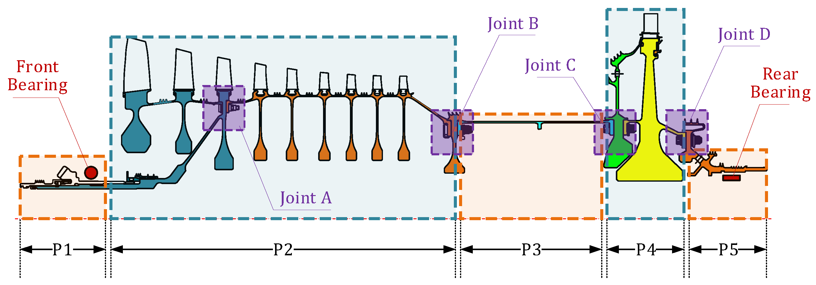
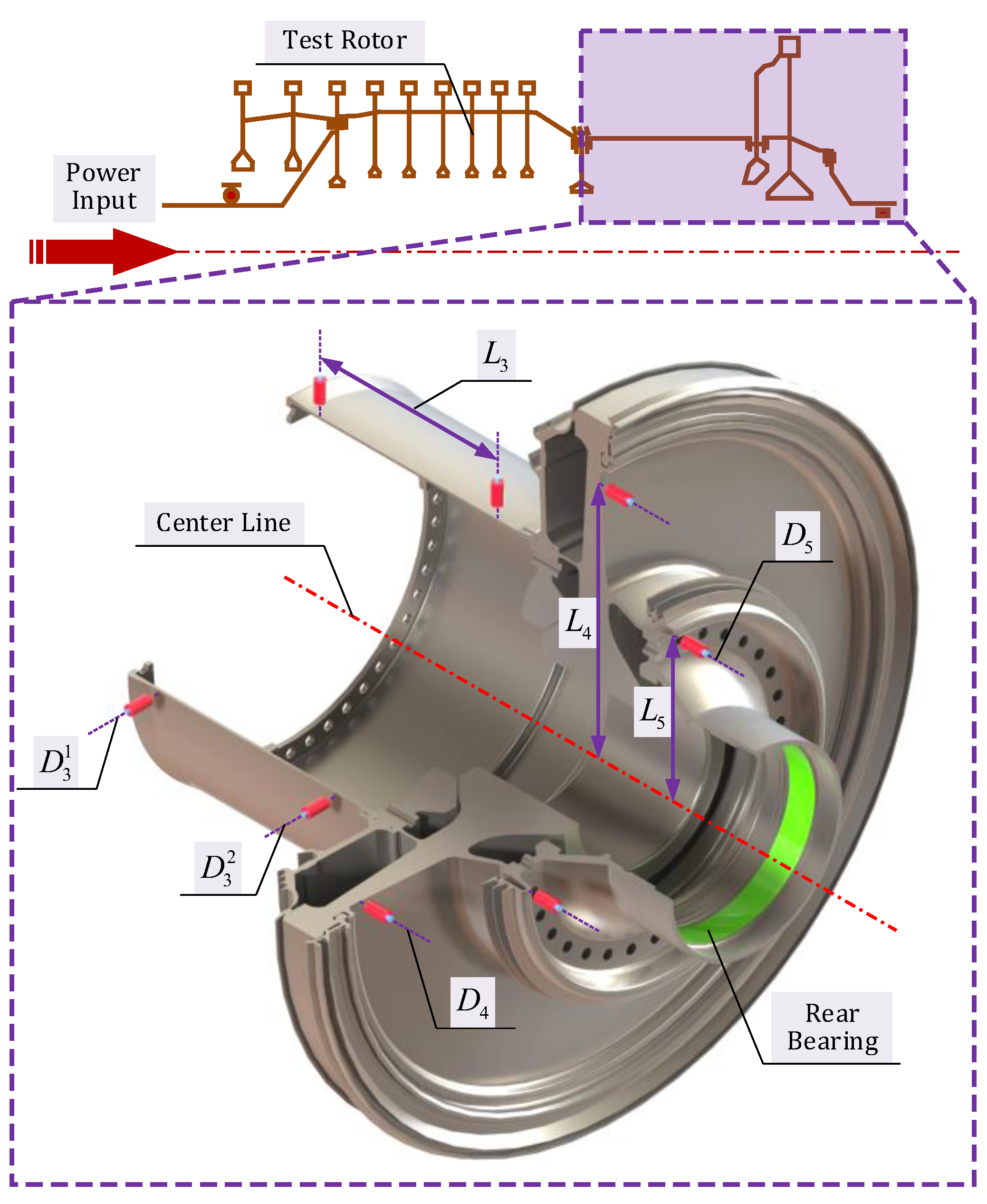
2.1. Configuration of a Typical High-Speed Jointed Rotor

Figure 1 illustrates a typical high-speed jointed rotor system consisting of multiple components interconnected axially through joints. The inherent variations in materials and geometric configurations among these components lead to inevitable changes in their relative angular positions during high operational speeds, resulting in distinct motions of these components. Consequently, the rotational inertia load excitations arising from these motions also undergo corresponding changes. Therefore, the rotor no longer complies with the assumption of being in constant state.
Based on the structural characteristics of the rotor and its deformations during operation, certain connecting components that share similar characteristics and motion states can be aggregated and represented as unified entities, denoted as “structural elements” or simply “elements” for conciseness. These elements can be classified into two categories based on their mass and stiffness: “mass elements” and “elastic elements”. “Mass elements” refer to elements with large mass and moments of inertia, whose own deformations can be neglected during motion. In the rotor system, the compressor element (P2) and turbine element (P4) are both considered as mass elements. Meanwhile, “elastic elements” refer to elements with a smaller mass but significant deformations, which determine the stiffness of the rotor system. In this rotor, the front shaft element (P1), drum shaft element (P3), and rear shaft element (P5) are all classified as elastic elements.

2.2. Description of the Rotational Inertia Load Distributed in the Rotor

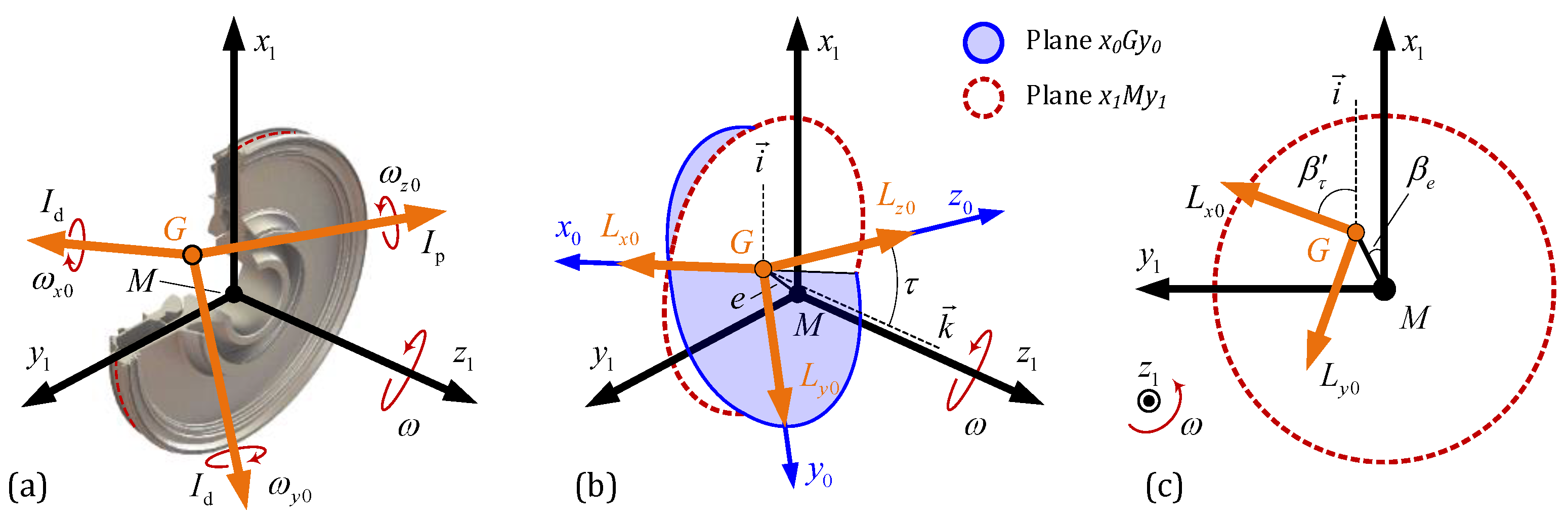
2.2.1. Description Method Based on PAI Slant and CM Offset

In a rotating rotor, its elements experience non-inertial motion, leading to continuous changes in their linear and angular momentum due to the constraints imposed by bearings. Consequently, the rotor generates reaction forces on the constrained boundaries, known as rotational inertia loads, which can be expressed as
{ F I = ρ ( a ) d V = d P / d t M I = ρ r × ( a ) d V = d L / d t
where, F I , M I —rotational inertial force and rotational inertia moment generated by the element, respectively, a —acceleration of the element, r —displacement vector of the element relative to its centroid, and P , L —linear and angular momentum of the element.
Obviously, an element’s linear momentum is determined by its mass and velocity, while its angular momentum is determined by its moment of inertia and angular velocity. As shown in Figure 2, it is assumed that the rotor’s elements are geometrically symmetrical, but due to manufacturing and assembly errors, its CM, referred as G , does not coincide exactly with its centroid, referred as M . Similarly, the polar PAI, referred as I p , does not coincide exactly with the rotor’s rotation axis. Therefore, it is necessary to establish two coordinate systems, one of which is a body-fixed translation coordinate system x 1 M y 1 , based on M , while the other is based on G , seen in Figure 2b as x 0 G y 0 . These two coordinate systems are used to describe the mass asymmetry of the element and its linear momentum and angular momentum during rotation. It is worth noting that this paper assumes that the rotor motion is always synchronized and in the forward direction.
Among them, the distance between G and M is called the eccentricity distance, denoted as e ; the angle between G M ¯ and M x 1 is called the eccentric phase angle, denoted as β e . During the rotation of the element, the position of its CM in coordinate x 1 M y 1 can be represented as
{ x 1 = e cos ( ω t + β e ) y 1 = e sin ( ω t + β e ) z 1 = const
Substituting Equation (2) into Equation (1), the expression for the rotational inertia force can be obtained as
{ F I , x = d P x / d t = m e ω 2 cos ( ω t + β e ) F I , y = d P y / d t = m e ω 2 sin ( ω t + β e )
Based on the geometric relationship, the expressions for the components of the rotor’s self-rotation ω in the coordinate x 0 G y 0 can be obtained as
( ω x 0 ω y 0 ω z 0 ) = A T ( 0 0 ω )
where, A is a transformation matrix to transfer vectors in coordinate x 0 G y 0 to x 1 M y 1 . Assuming the initial phase of the motion of coordinate x 0 G y 0 relative to coordinate x 1 M y 1 is 0, and A can be expressed as
A = ( cos ( ω t ) sin ( ω t ) 0 sin ( ω t ) cos ( ω t ) 0 0 0 1 ) ( cos β τ sin β τ τ sin β τ sin β τ cos β τ τ cos β τ 0 τ 1 )
by which the angular momentum vector L 0 = ( L x 0 , L y 0 , L z 0 ) T of this element in coordinate x 0 G y 0 can be obtained as
( L x 0 L y 0 L z 0 ) = I ( ω x 0 ω y 0 ω z 0 ) = I A T ( 0 0 ω )
where, I represents the matrix of the moment of inertia, and it can be expressed as
I = d i a g ( I d , I d , I p )
Transforming L 0 into coordinate x i M y i , which can be expressed as
( L x 1 L y 1 L z 1 ) = A I A T ( 0 0 ω )
Neglecting the term containing higher-order small quantities τ 2 , the angular momentum of the element can finally be obtained as
( L x 1 L y 1 L z 1 ) = ( ( I d I p ) τ ω sin ( ω t + β τ ) ( I d I p ) τ ω cos ( ω t + β τ ) I p ω )
Substituting Equation (9) into Equation (1), the rotational inertia moment can be obtained as
{ M I , x = d L x 1 / d t = ( I d I p ) τ ω 2 cos ( ω t + β τ ) M I , y = d L y 1 / d t = ( I d I p ) τ ω 2 sin ( ω t + β τ )
Combining Equations (3) and (10), then expressing them in terms of complex notation, the expression for rotational inertia load excitation can be obtained as
{ F ˜ I = m e ˜ ω 2 e i ω t M ˜ I = ( I d I p ) τ ˜ ω 2 e i ω t
where, e ˜ = e β e , τ ˜ = τ β τ , β τ = β τ π / 2 , and from a geometric perspective, β τ represents the angle between the plane containing the PAI slant and plane x 1 M y 1 .
From Equation (11), it can be seen that the rotational inertia force F ˜ I depends on the mass and CM offset of the element, while the rotational inertia moment M ˜ I not only depends on the slant of the element’s PAI τ ˜ but also on the relative size of the polar and diametral moments of inertia. Therefore, the elements that satisfy I p < I d are referred to as thick-disks, while those that satisfy I p > I d are referred to as thin-disks. These two types of rotors exhibit significant differences in the direction and variation of the rotational inertia moment with the operational speed [14].

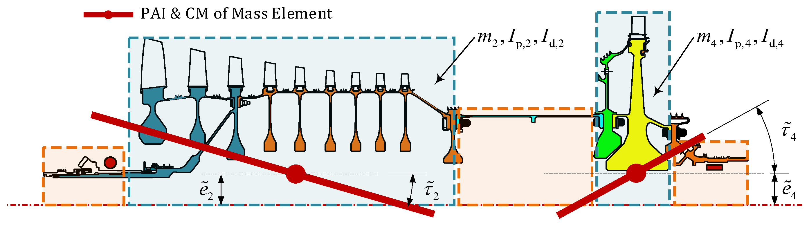
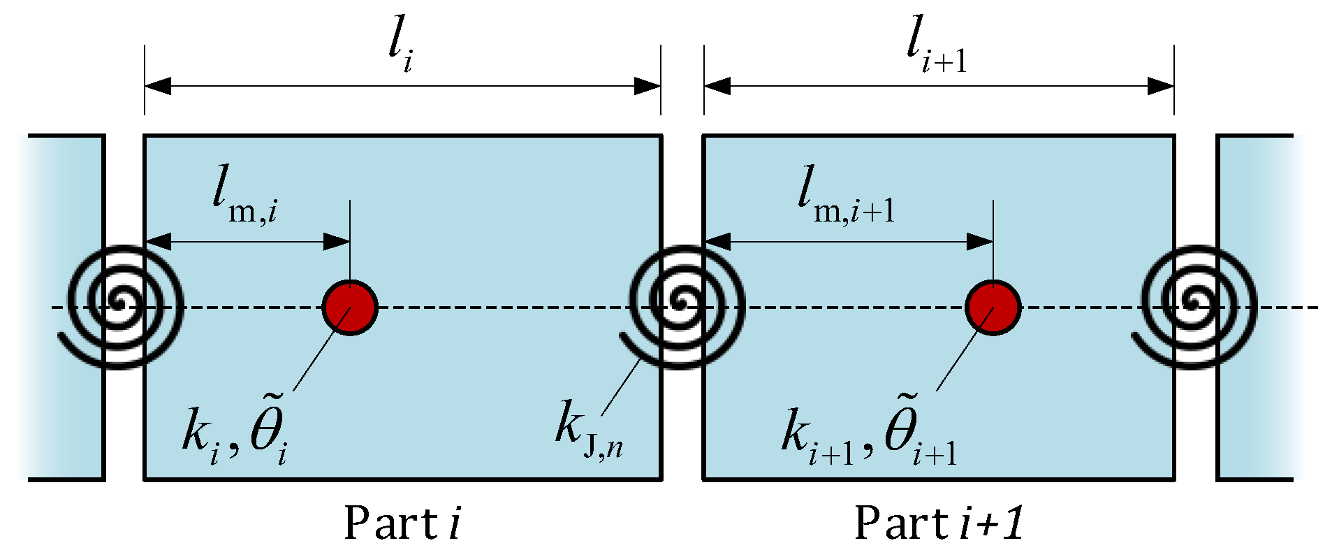
2.2.2. Axial Distribution of the Rotational Inertia Load of a Rotor

In high-speed rotors, because most of the mass and the moment of inertia are concentrated in the compressor and turbine elements, only the mass asymmetry of these two mass elements should be considered. However, the compressor element is typically a thick-disk, while the turbine element is a thin-disk, resulting in significant differences in the direction and variation patterns of the rotational inertia loads generated by their rotations at varying operational speeds. If the compressor and turbine element are treated as a single entity and combine their unbalances, it would not accurately represent the actual state of the rotational inertia loads acting on the rotor.
Therefore, as shown in Figure 3, it is necessary to describe the unbalance of the compressor and turbine elements separately by using the CM offset e ˜ 2 , e ˜ 4 and the PAI slant τ ˜ 2 , τ ˜ 4 , based on which the rotational inertia loads applied to the rotor can be described as
{ F ˜ 2 = m 2 e ˜ 2 ω 2 e i ω t , M ˜ 2 = ( I d , 2 I p , 2 ) τ ˜ 2 ω 2 e i ω t F ˜ 3 = m 3 e ˜ 3 ω 2 e i ω t , M ˜ 3 = ( I d , 3 I p , 3 ) τ ˜ 3 ω 2 e i ω t
where F ˜ 2 , M ˜ 2 and F ˜ 4 , M ˜ 4 represent the rotational inertia force and rotational inertia moment generated by the compressor element and the turbine element. These rotational inertia load excitations act on elements’ CM.

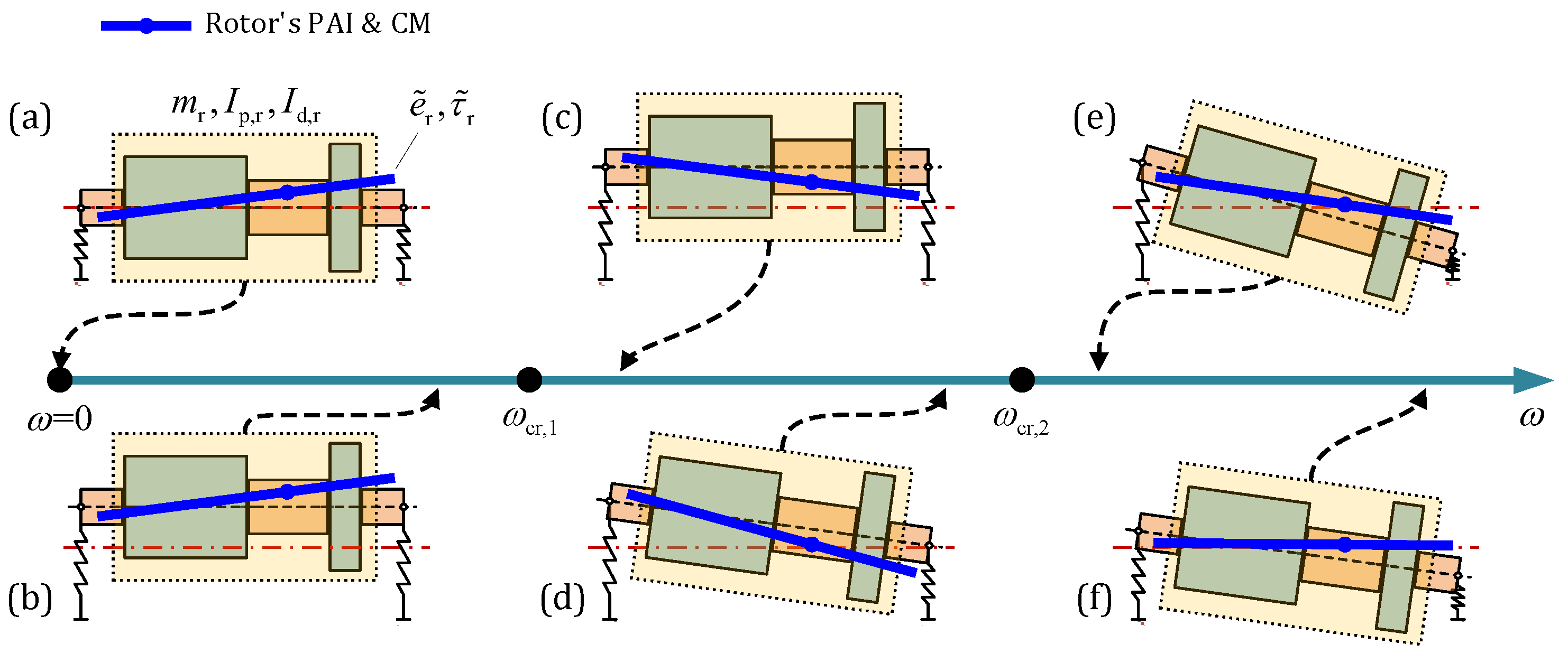
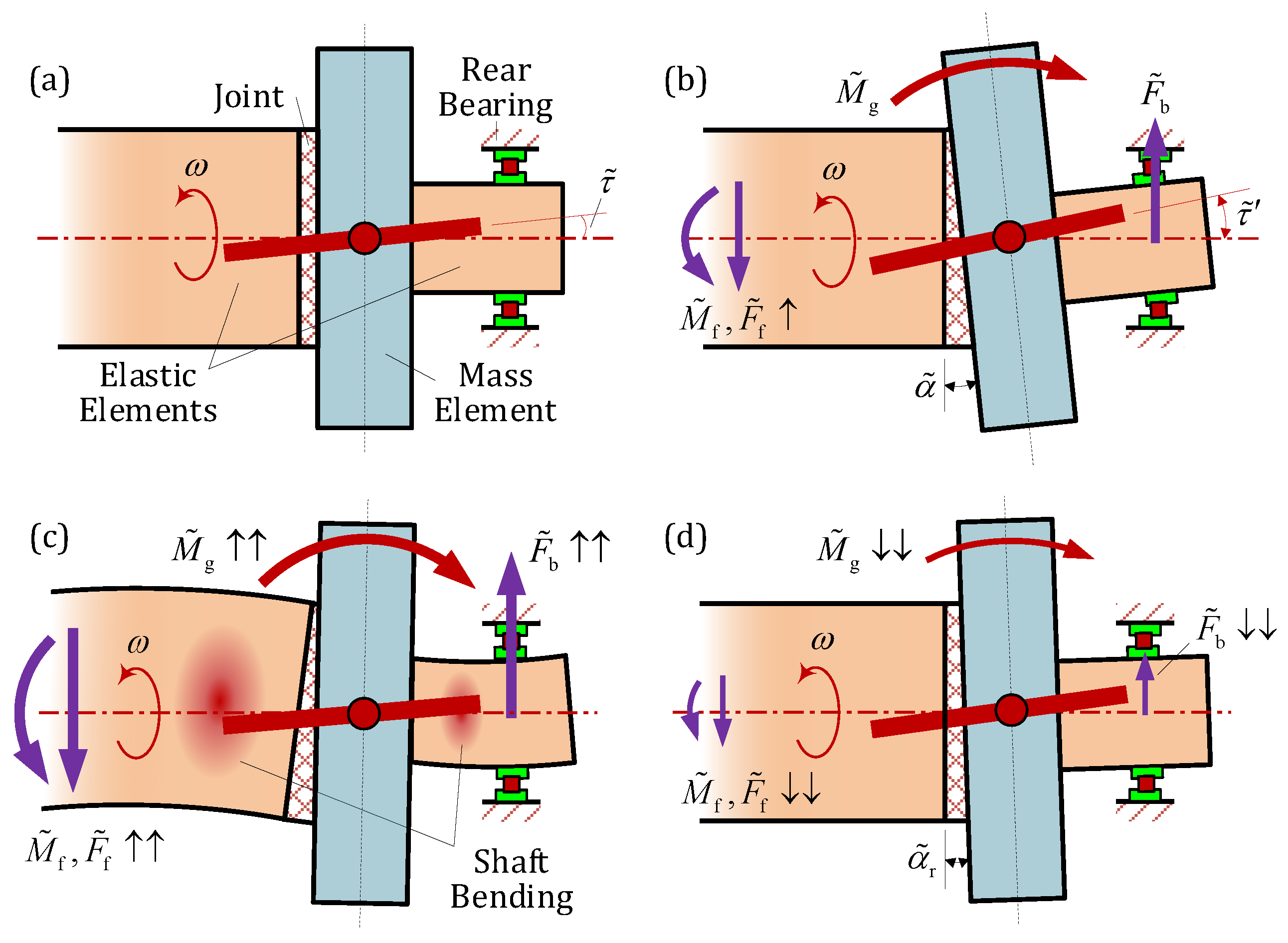
2.3. Influence of the Motion State of the Rotor

As illustrated in Figure 4, the motion of the rotor in the low-speed range is depicted with respect to the operational speed. In this low-speed region, the effect of rotor bending deformation on the relative positions between elements can be negligible. Therefore, the rotor can be treated as a thick-disk rotor due to I p , r < I d , r . The mass asymmetry of the compressor and the turbine elements are aggregated and represented as the rotor’s CM offset e ˜ r and PAI slant τ ˜ r . The rotor’s motion state variation with the operational speed ω can be described using a four degrees-of-freedom rotor model [15]. Specifically, before reaching the critical speed, the amplitude of the rotor dynamic response increases with ω . However, after surpassing the critical speed, the dynamic response decreases with ω due to a turning inwards of the rotor’s CM or PAI.
As illustrated in Figure 5, the motion of the rotor in the high-speed range shows significant changes due to rotor bending deformation and the corresponding alterations in the relative positions between its mass elements. Consequently, the rotor can no longer be considered as a constant-state rotor, and it becomes imperative to separately consider the mass asymmetry and rotational inertia load excitations for the compressor element and the turbine element, respectively. Notably, the turbine element is classified as a thin-disk, where the effect of rotational inertia moment is relatively strong, by which the turbine element undergoes angular displacement, gradually approaching and aligning its PAI with the rotor’s rotation axis. Subsequently, the angular deformation of the turbine element ceases to exhibit significant increments with further increases in ω . Moreover, with a further increase in ω , the rotational inertia moment generated by the compressor element also becomes significant, causing its PAI to align with the rotor’s rotation axis.
Hence, from the comprehensive analysis presented, it can be deduced that at high-speed range, the rotor experiences bending deformation, resulting in alterations in the relative angular positions between the compressor element and the turbine element. This, in turn, impacts the rotor’s mass asymmetry, leading to the manifestation of localized rotational inertia load excitations caused by elements’ mass asymmetry.

2.4. Influence of the Mechanical Characteristic of the Joints

2.4.1. Bending Stiffness Loss of the Joints

The impact of operational loads, such as centrifugal forces, thermal deformations, bending moments, and aerodynamic loads, can lead to changes in the contacting area and redistribution of contact stresses at the joints’ interfaces, resulting in a reduction in their bending stiffness [30,31,32]. Consequently, in the high-speed range, the bending deformation of the rotor can become more pronounced due to the weakened bending stiffness of its joints. This alteration in the rotor’s bending behavior affects the distribution of rotational inertia load excitations and subsequently influences the rotor’s dynamic response.
As shown in Figure 6, taking the bending stiffness of Joints C/D ( k J , C , k J , D ) as examples, the influence of joints’ bending stiffness loss on the distribution of the rotational inertia loads in the high-speed range ( ω > ω cr , 2 ) can be concluded as follows:
(a) When k J , C > k J , D : As k J , C determines the bending stiffness between the compressor element and the turbine element, a higher k J , C can effectively restrains the angular dislocation between the turbine element and the compressor element, by which the integrity of the rotor is enhanced. Therefore, the rotor can still be regarded as a thick-disk, whose rotational inertia moment excitation M ˜ g , r decreases with the operational speed. Simultaneously, the decrease in k J , D weakens the bearing constraint exerted on the rotor motion, and this weakening in constraint reduces the reaction forces at the rear bearing.
(b) When k J , C < k J , D : A lower value of k J , C exacerbates the change in the relative position between the compressor and turbine elements, leading to the appearance of local rotational inertia moment excitation, denoted as M ˜ g , 4 , caused by the slant of the turbine element’s PAI. This rotational inertia moment excitation can rapidly increase with the operational speed. Simultaneously, a higher k J , D imposes stronger constraints on the rotor motion, inducing a significant increase in the bearing load in the high-speed range.

2.4.2. Sudden Angular Deformation

During the variation of operational conditions, the joints may experience non-uniform interface constraints or be subjected to bending moments, leading to changes in the distribution of interface contact stresses or macroscopic interfacial slide, resulting in angular deformation of the joints [28,29]. This, in turn, causes additional slant of the PAI of nearby mass elements, as depicted in Figure 7. To accurately account for the effect of the angular deformation of the joints on the slant of the PAI of the mass element and the resulting rotational inertia moment, it is necessary to modify Equation (12) as
{ F ˜ 2 = m 2 e ˜ 2 ω 2 e i ω t , M ˜ 2 = ( I d , 2 I p , 2 ) τ ˜ 2 ω 2 e i ω t F ˜ 4 = m 4 e ˜ 4 ω 2 e i ω t , M ˜ 4 = ( I d , 4 I p , 4 ) τ ˜ 4 ω 2 e i ω t
where, τ ˜ 2 , τ ˜ 4 represents the slant angles of the compressor element and the turbine element, respectively, considering the influence of the angular deformation of the joints, and they are denoted as τ ˜ 2 = τ ˜ 2 + α ˜ 2 and τ ˜ 4 = τ ˜ 4 + α ˜ 4 .
It is critical to note that the mechanical characteristics of the joints’ interfaces are discontinuous, resulting in sudden changes in interface contact stress and sliding damage with varying operational loads. Therefore, the impact of angular deformation of the joint on the rotational inertia load distribution of the elements also exhibits abrupt changes.

3. Dynamic Model for High-Speed Jointed Rotor System

3.1. Parameters of Rotor System

As shown in Figure 8, the rotor’s motion state is achieved by the lateral displacement r ˜ i and angular displacement θ ˜ i of each element’s CM, denoted as
u = ( , r ˜ i , θ ˜ i , ) T
where, u represents the displacement vector of the rotor system. To analyze the dynamic response of the high-speed jointed rotor, it is necessary to obtain the mass, moment of inertia, and bending stiffness of its constituent element, i.e., m i , I p , i , I d , i , k θ , i shown in Figure 8, as well as the bending stiffness of the joints k J , i . The boundary conditions of the rotor, namely the stiffness k bf , k br and damping coefficients c bf , c br of the front and rear bearings also need to be considered. Additionally, the CM offsets and PAI slants in the mass elements, denoted as e ˜ 2 , τ ˜ 2 , e ˜ 4 , τ ˜ 4 , must be considered.

3.2. Rotor Motion Differential Equations Based on Lagrange’s Method

Based on the above-mentioned description method, the motion differential equations of this rotor system can be obtained using Lagrange’s method as
d d t L u ˙ i L u i = Q i
where, L can be expressed as
L = i = 1 n T i ( i = 1 n 1 V i , i + 1 + V bf + V br )
where, T i —kinetic energy of the i th degree of freedom (DoF), V i , i + 1 —elastic energy between the i th and ( i + 1 ) th DoF, V bf , V br —elastic energy of front and rear bearings, u i —displacement of the i th DoF, Q i —generalized force applied to the i th DoF.
Based on Equation (15), the mass matrix M, damping matrix C , and stiffness matrix K of the rotor system can be obtained, and simultaneously, the motion differential equations of this rotor system can be expressed as
M u ¨ + C u ˙ + K u = Q
where the vector of generalized force can be obtained by Equation (13) as
Q = ( , F ˜ 2 , M ˜ 2 , , F ˜ 4 , M ˜ 4 , ) T

3.3. Mechanical Characteristics of Joints in the Dynamic Rotor Model

3.3.1. Bending Stiffness Loss of the Joints

In order to characterize the influence of the joints’ bending stiffness loss on the rotor dynamic model, the stiffness matrix K in Equation (17) needs to be modified. As shown in Figure 9, the bending stiffness between the i th and ( i + 1 ) th elements’ angular DoF, denoted as k t , i , i + 1 , can be considered as a series connection of the bending stiffness of the i th element’s rear section k θ , i r , the bending stiffness of the ( i + 1 ) th element’s front section k θ , i + 1 f , and the bending stiffness of the joint between the two elements k J , n . Therefore, k t , i , i + 1 can be expressed as
1 k t , i , i + 1 = 1 k θ , i r + 1 k θ , i + 1 f + 1 k J , n
Assuming that the elements are constant section beams, it is easy to determine the bending stiffness of the front and rear sections of the i th element by Equation (20)
k θ , i f = l i l m , i k θ , i , k θ , i r = l i l i l m , i k θ , i
Meanwhile, the stiffness loss coefficient β n is used to represent the degree of stiffness loss at the n th joint by
β n = 1 k J , n / k J , n 0
where, k J , n 0 —bending stiffness of the joint when its interfaces are perfected merged, k J , n —actual bending stiffness of the joint.

3.3.2. Sudden Angular Deformation of the Joint

Due to the turbine element having a configuration of a thin-disk, the impact of its rotational inertia moment is more pronounced. Furthermore, Joint C is subjected to harsh loading conditions, making it more susceptible to deformation during operation. As a result, this paper specifically investigates the influence of the angular deformation of Joint C on the rotational inertia moment excitation caused by the turbine element.
As shown in Figure 10, for a turbine element with an initial PAI slant τ ˜ , when the initial slant is small and the operational speed ω is low, the rotational inertia moment generated by the turbine element and the resulting bending deformation of the rotor can almost be neglected. However, as ω increases, various loads such as centrifugal force, axial tension force, and thermal deformation acting on the joints gradually increase with ω , until ω reaches a certain threshold ω t . At this key point, the contact stress distribution or interface slip damage at the joint’s interfaces experiences a sudden change, leading to a sudden angular deformation in this joint, denoted as α ˜ . As a result, the PAI slant of the turbine element suddenly increases to τ ˜ . It can be assumed that the additional slant of the turbine element’s PAI equals the joint’s angular deformation, which can be expressed as
τ ˜ = τ ˜ + α ˜
In response, the rotational inertia moment excitation generated by the turbine element also suddenly increases to M ˜ g . This rotational inertia moment acts on the two adjacent elastic elements, causing bending deformations in these elements. As the rear bearing acts as a constraint boundary, it can generate a significant reaction force, denoted as F ˜ b , that balances the bending deformations in the elastic elements. Additionally, apart from inducing elastic elements’ bending deformations and bearing loads, the rotational inertia moment also applies a bending moment, denoted as M ˜ J , to the joint. Force equilibrium can be formulated as
M ˜ J = M ˜ g + l ˜ s × F ˜ b
where, l ˜ s —position vector of the rear bearing relative to the CM of the turbine element.
As ω increases, the rotational inertia moment rapidly increases and the turbine element’s PAI tends to align with the rotor’s rotation axis. However, when M ˜ J acting on the joint reaches the threshold, denoted as M t , the joint can undergo a sudden angular deformation in the same direction as M ˜ J , resulting in a residual angular deformation α ˜ r . As a result, the angle between the turbine element’s PAI and the rotor’s rotation axis suddenly decreases, leading to a sharp reduction in the rotational inertia moment generated by the turbine element. Consequently, the rotor’s bending deformation and the corresponding bearing loads also experience a sudden decrease.
Therefore, the angular deformation of the turbine front joint, denoted as α ˜ C , is expressed as a piecewise function of ω and the bending moment applied to Joint C (denoted as M ˜ J , C ) given by
α ˜ C ( ω , M ˜ J , C ) = { 0 , ω < ω t α ˜ , ω ω t & | M ˜ J , C | < M t , C α ˜ r , | M ˜ J , C | M t , C
where ω t —threshold operational speed at which Joint C undergoes a sudden increase in angular deformation, and M t , C —threshold bending moment at which Joint C undergoes a sudden angular deformation decrease. These threshold values can be obtained through static analysis of the bolt joint. By substituting Equation (24) into Equation (13), the impact of the sudden angular deformation caused by the bolt joint on the rotor’s dynamics can be analyzed.

4. Simulation of High-Speed Jointed Rotor System

Table 1 presents the mass, moment of inertia, and bending stiffness values of the rotor and its elements. The stiffnesses of the front and rear bearings are set as k bf = 5 × 10 7   N / m and k br = 1 × 10 8   N / m . Moreover, the local bending stiffnesses of the bolt joints are obtained through static mechanical analysis.

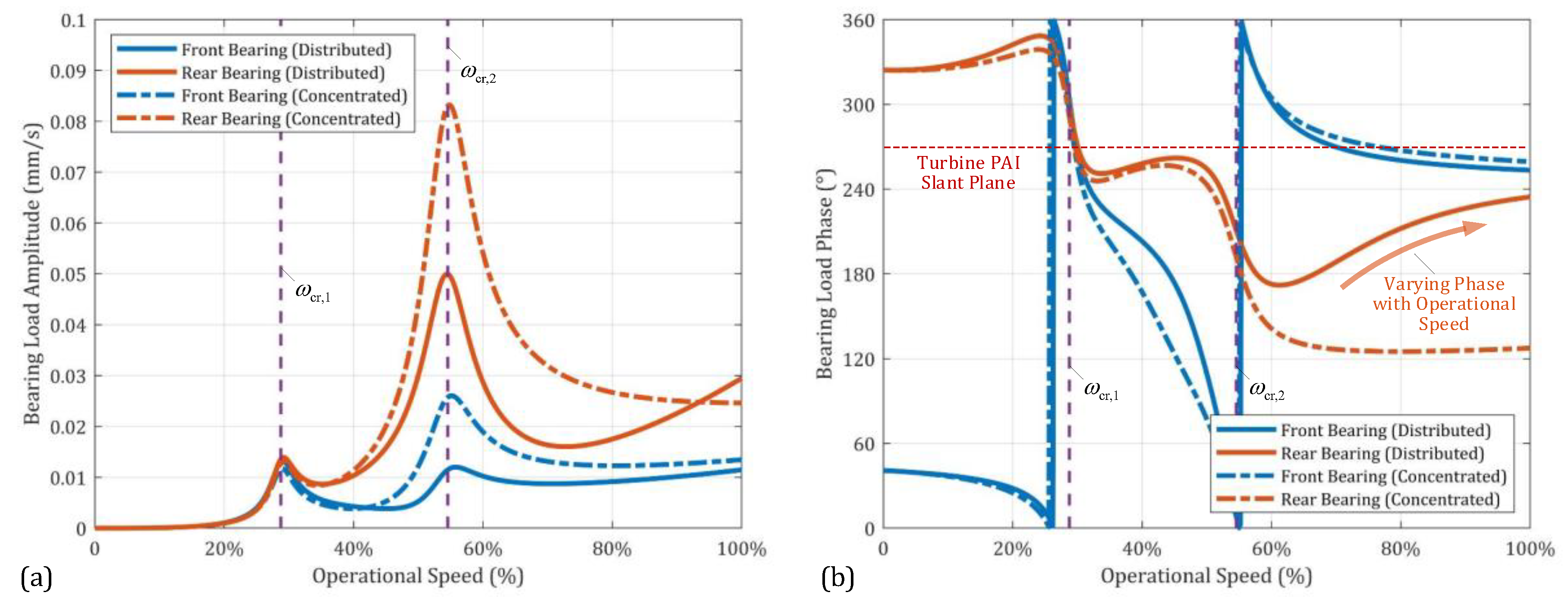
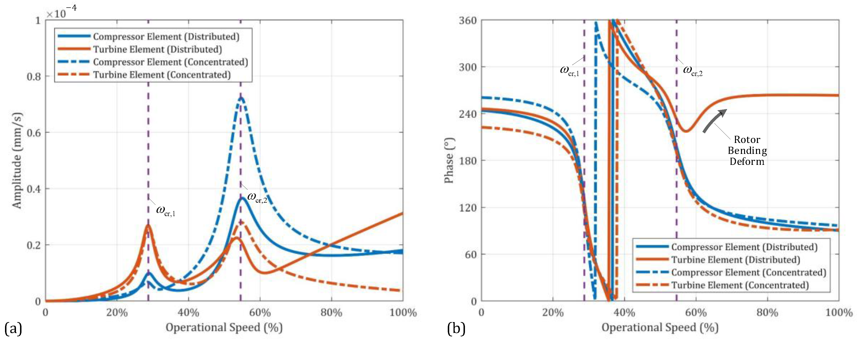
4.1. Rotor Dynamic Response with Different Excitation Model

The influence of sudden angular deformation of the rotor joints is temporarily ignored and the distributed rotor unbalance state can be set as e ˜ 2 m 2 = e ˜ 4 m 4 = 300   g mm 0 ° , τ ˜ 2 = 0 0 ° , and τ ˜ 4 = 1 × 10 4 90 °   rad , referred as Group A.
Meanwhile, in order to compare the effects of different excitation models on rotor dynamics, this section also designs a second group of rotor unbalance states, referred to as Group B. In this Group B, the CM offset of the mass element remains unchanged, and the mass elements’ PAI slants are equivalent to the CM offset, denoted as Δ e ˜ 2 m 2 , Δ e ˜ 4 m 4 , in the planes of the compressor and turbine elements’ CM. Based on force balance, Δ e ˜ 2 m 2 , Δ e ˜ 4 m 4 can be obtained by Equations (25) and (26), where L ˜ 24 represents the vector between the turbine element’s CM and the compressor element’s CM.
L ˜ 24 × Δ e ˜ 4 m 4 = ( I d , 2 I p , 2 ) τ ˜ 2 + ( I d , 4 I p , 4 ) τ ˜ 4
Δ e ˜ 2 m 2 + Δ e ˜ 4 m 4 = 0
Clearly, in Group B, the rotor’s mass asymmetries, regardless of their types or locations, are represented as the rotor’s dynamic unbalance, denoted as ( e ˜ 2 + Δ e ˜ 2 ) m 2 and ( e ˜ 4 + Δ e ˜ 4 ) m 4 . This unbalance equivalent method considers the rotor as a four degrees-of-freedom rotor, and the distributed rotational inertia load excitations caused by mass elements’ CM offset and PAI slant are consolidated into two planes.
The results of comparing the rotor’s dynamic response under the two excitation models are depicted in Figure 11. It is evident that when using the concentrated excitation model, the front and rear bearing loads of the rotor follow a trend where the bearing load amplitude increases with the operational speed, reaches a maximum at the critical speed, and then decreases with further increase in operational speed. As the rotor approaches its maximum operating speed, the bearing load remains relatively constant. Additionally, upon observing the phase of the bearing load, it can be inferred that within the non-critical speed region, the vibration phase of both the front and rear bearing remains nearly constant with the operational speed, and the phase difference between the front and rear bearing remains consistent, which aligns with the predictions of the four degrees-of-freedom rotor model.
When utilizing the distributed excitation model, in the low-speed range ( ω < ω cr , 2 ), the rotor bearing loads, both in terms of amplitude and phase, exhibit a pattern nearly identical to that of the concentrated excitation model group. This similarity arises because, at this low-speed range, the rotor undergoes no significant bending deformation, allowing it to be treated as having integrity, and thus, the dynamic response of the rotor remains similar for different rotational inertia load excitation models. However, as the rotational speed enters the high-speed range ( ω > ω cr , 2 ), the rotational inertia moment generated by the turbine element increases continuously with the operational speed, leading to a rapid increase in the amplitude of the bearing load with the operational speed (referred to as vibration following, or VF). Furthermore, the phase of the rear bearing load also rapidly approaches the plane of the turbine element’s PAI slant (90/270° plane) with increasing operational speed.
The angular displacements of the mass elements under different excitation models are illustrated in Figure 12. In the low-speed range ( ω < ω cr , 2 ), it can be observed from Figure 12a that the excitation model has little influence on the amplitude of the angular displacements of the mass elements. However, as the operational speed enters the high-speed range ( ω > ω cr , 2 ), using the concentrated excitation model results in both the compressor element and turbine element experiencing a decrease in their angular displacements with increasing operational speed, while their difference in angular displacements remains almost unchanged. This indicates that the rotor undergoes little bending deformation in this speed range. However, when the distributed excitation model is used, the turbine element experiences a significant local rotational inertia moment, leading to an increase in its angular displacement with the operational speed. Furthermore, the difference in angular displacements between the turbine element and the compressor element increases rapidly with the operational speed, suggesting that the bending deformation of the rotor is progressively intensifying.
From Figure 12b, it can be observed that when using the concentrated excitation model, the angular displacements of the compressor element and turbine element occur in the same plane throughout the entire speed range, which confirms the rotor’s integrity and minimal bending deformation. However, when the distributed excitation model is used, the phase difference of the turbine element’s angular displacement relative to that of the compressor element rapidly changes by 180° as the operational speed exceeds the second critical speed. This confirms the conclusion that the bending deformation of the rotor significantly intensifies under the distributed excitation model, leading to substantial changes in the relative positions of the mass elements.

4.2. Impact of Joint Bending Stiffness on Rotor Dynamics

Since the turbine element is a thin-disk, the rotational inertia load it generates is more sensitive to the angular deformation of nearby joints. Therefore, this section primarily focuses on investigating the impact of the bending stiffness loss in the bolt joints before and after the turbine element.
To make the analysis results more general, parameter λ is defined as the ratio of the bending stiffnesses of the front and rear bolt joints of the turbine element., i.e., λ = k J , C / k J , D , where k J , C represents the bending stiffnesses of the joints before the turbine element, and k J , D represents the bending stiffnesses of the joints after the turbine element. While keeping k J , D constant, the rotor’s bearing loads as λ = 0.5 ,   1.0 ,   2.0 ,   5.0 are solved. The results are illustrated in Figure 13. Based on this figure, conclusions can be made:
(a) As the bending stiffnesses of the rotor’s joints change, the first two critical speeds of the rotor also change, but the variation is relatively small (less than 10%). This is because the modal shapes corresponding to the first two critical speeds are rigid body modes, which makes them less sensitive to changes in rotor bending stiffness;
(b) In the low-speed range ( ω < ω cr , 2 ), the rotor’s bearing loads are not sensitive to changes in joints’ bending stiffness. This is because the rotor does not undergo significant bending deformation within this speed range. However, it should be noted that near the second critical speed, with an increase in k J , C , the bearing loads at the second critical speed rapidly increase. This is because the second critical speed corresponds to a rotor’s pitching modal shape, and an increase in bending stiffness improves the integrity of the rotor. This enables the rotational inertia moment caused by the turbine element to act on the entire rotor, leading to a significant increase in this modal vibration.
(c) In the high-speed range ( ω > ω cr , 2 ), the amplitude of the rear bearing loads is extremely sensitive to the joints’ bending stiffness. When k J , C is low, the rear bearing loads can continuously increase with the operational speed. The reason behind this phenomenon is that as the k J , C decreases, the integrity of the rotor is also weakened, resulting in the manifestation of the rotational inertia moment excitation caused by the turbine element’s PAI slant. This rotational moment rapidly increases with the operational speed, leading to an increase in the rear bearing loads, which is consistent with the analysis in Section 2.4.1.
In addition, both the concentrated excitation model and the distributed excitation model were employed to solve the rotor’s dynamic characteristics. To assess the influence of different excitation models on the simulation results, the error coefficient η E ( ω ) was introduced, which is defined as
η E ( ω ) = ( F br , con ( ω ) F br , dis ( ω ) ) / F br , dis ( ω )
where F br , con ( ω ) , F br , dis ( ω ) represent the amplitudes of rear bearing loads obtained by employing the concentrated excitation model and the distributed excitation model, respectively. The curves of the error coefficient η E ( ω ) are illustrated in Figure 14.
It can be observed that when the operational speed is low or close to the first critical speed, employing either the concentrated excitation model or the distributed excitation model has little impact on the prediction of the rotor’s dynamic response. However, in the high-speed range, there is a significant difference in the rotor’s dynamic response characteristics obtained from the two excitation models. If the concentrated excitation model is employed instead of the distributed excitation model in this speed range, the rotor’s dynamic response characteristics will be greatly underestimated. Moreover, when the bending stiffness of the joints between the compressor element and the turbine element is low, the poor integrity of the rotor can result in a more severe underestimation of the rotor’s dynamic response in this high-speed range. Therefore, it is essential to consider the influence of joint bending stiffness and use the distributed excitation model for accurate prediction of the rotor’s dynamic response in the high-speed range.

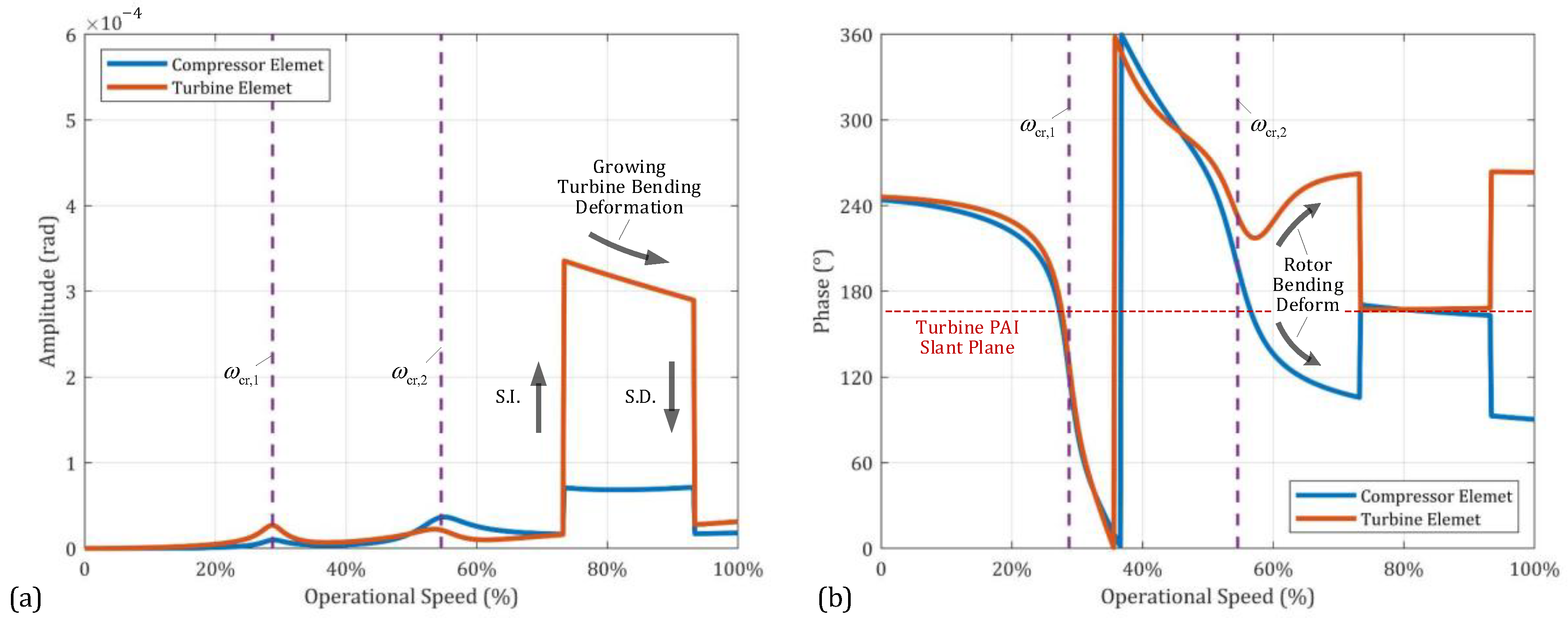
4.3. Impact of Joints’ Angular Deformation on Rotor Dynamics

Employing Group A as the rotor’s unbalance state, let ω t = 72 % ω max , M t = 1400   N m , α ˜ = 3 × 10 4 165 °   rad , α ˜ r = 0 0 ° . The simulation results of the rotor dynamic response are illustrated in Figure 15.
From Figure 15a, it can be observed that the rotor’s dynamic response increases with the operational speed until it reaches its maximum value at the first/second critical speed, then decreases with the operational speed. However, when the rotor’s operational speed satisfies ω = ω t , there is a sudden angular deformation in Joint C, causing the turbine element to slant. The resulting rotational inertia moment suddenly increases the bearing loads, especially for the rear bearing, which is closer to the turbine element. As the turbine element is a thin-disk, the rotational inertia moment it generates can increase with the operational speed even under this supercritical state, and this increasing rotational inertia moment leads to a speed-dependent increase in the bearing load. The vibration following continues until the rotational inertia moment generated by the turbine element becomes large enough that it makes M ˜ J ( ω ) satisfy | M ˜ J ( ω ) | = M t . At this point, the angular deformation of Joint C suddenly recovers, causing the turbine element’s PAI to coincide with the rotor’s rotation axis, i.e., “straightened”, leading to a sudden decrease in bearing loads.
Furthermore, from Figure 15b, it can be noticed that at the moment when the rotor’s dynamic response experiences a sudden increase, the phase of the front and rear bearing loads abruptly shifts towards the plane where the additional PAI slant of the turbine element occurs (165/345° plane), and with increasing operational speed, it gradually approaches this plane. This is because after the joint angular deformation induces a significant PAI slant of the turbine element, the dominant factor influencing the rotor dynamics becomes the rotational inertia moment generated by the turbine element. As a result, the phase of the front and rear bearing loads abruptly shifts towards the plane where this rotational inertia moment or the additional PAI slant is located. Meanwhile, the amplitude of this moment can increase with the operational speed, causing the phase of the front and rear bearing loads to come closer and closer to this plane.
As the rotor’s operational speed increases, the variation of bending moments applied to different joints is illustrated in Figure 16. It can be observed that when Joint C undergoes a sudden angular deformation, the resulting spiked rotational inertia moment is caused by the turbine element, leading to a sudden increase in the bending moment applied to the rotor’s joints. Among them, Joint C experiences the highest bending moment. This is because this joint is the closest joint to the turbine element and has a higher bending stiffness. Furthermore, as the operational speed causes the rotational inertia moment generated by the turbine element to increase, the resulting bending moment applied to Joint C also increases until it reaches the threshold value M t , triggering this joint to angularly deform again. Consequently, the turbine element’s PAI slant disappears, leading to a sudden decrease in the bending moment applied to the rotor’s joints.
The angular displacement amplitudes and phases of the compressor and turbine elements are shown in Figure 17. By comparing with Figure 12, it can be observed that when ω = ω t , the deformation of Joint C causes a sudden increase in the angular displacement of the turbine element. However, the rotational inertia moment generated by the turbine element tends to restore the angular displacement of the turbine element. Therefore, as the operational speed increases, the angular displacement of the turbine element gradually decreases until the angular deformation of the joint suddenly recovers, causing the angular displacement of the turbine element to almost return to 0. In addition, by observing the phase of the angular displacement of the mass elements, it can be seen that at the moment of the sudden increase in the angular deformation of Joint C, the angular displacement of the mass element jumps to the plane where the additional slant of the turbine element’s PAI occurs (165/345° plane). This confirms that the deformation of the rotor in the high-speed range is dominated by the rotational inertia moment caused by the sudden additional slant of the turbine element’s PAI.

5. Dynamic Experiment of High-Speed Jointed Rotor System

5.1. Experimental Facility and Test Method

The experimental rotor used in this research is a full-scale rotor, constructed with materials and bearings identical to those utilized in real-world rotors. The rotor is driven by a high-speed motor at the front end. Acceleration sensors are installed at the front and rear bearings to measure the rotor bearing loads accurately. To capture the angular displacement of each element and the angular deformation of the joints as the operational speed changes, multiple sets of displacement sensors are placed at the turbine module. The arrangement of these displacement sensors at the turbine module is shown in Figure 18.
With the above-mentioned experimental setup, the lateral displacements of the drum shaft element, and the axial displacement of the turbine element and rear shaft element can be measured. The angular displacements of these elements can be obtained by
{ θ 3 , x = ( D 3 , x 2 D 3 , x 1 ) / L 3 θ 3 , y = ( D 3 , y 1 D 3 , y 2 ) / L 3
{ θ 4 , i = D 4 , i / L 4 θ 5 , i = D 5 , i / L 5   , i = x , y
where, θ 3 , i , θ 4 , i , and θ 5 , i represent the angular displacements of the drum shaft element, turbine element, and rear shaft element, respectively, in plane i ( i = x   or   y ). It can be assumed that the bending deformation of each element is relatively small, thus the angular deformation difference between adjacent element mainly comes from the bending deformation of the joints, which can be expressed as
{ α C , i = θ 4 , i θ 3 , i α D , i = θ 5 , i θ 4 , i   , i = x , y
where, α C , i , α D , i represent the angular deformations of Joint C and D, respectively, in plane i ( i = x   or   y ).

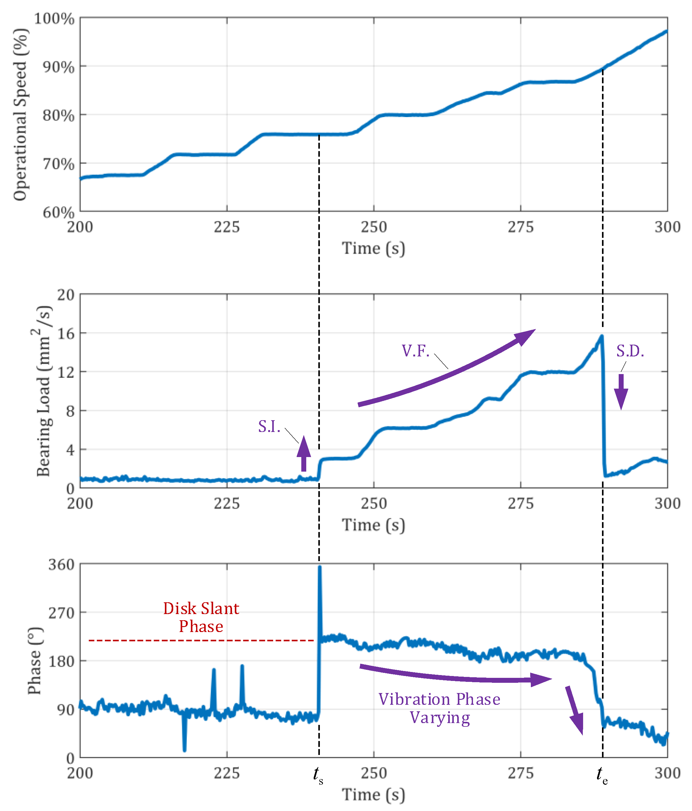
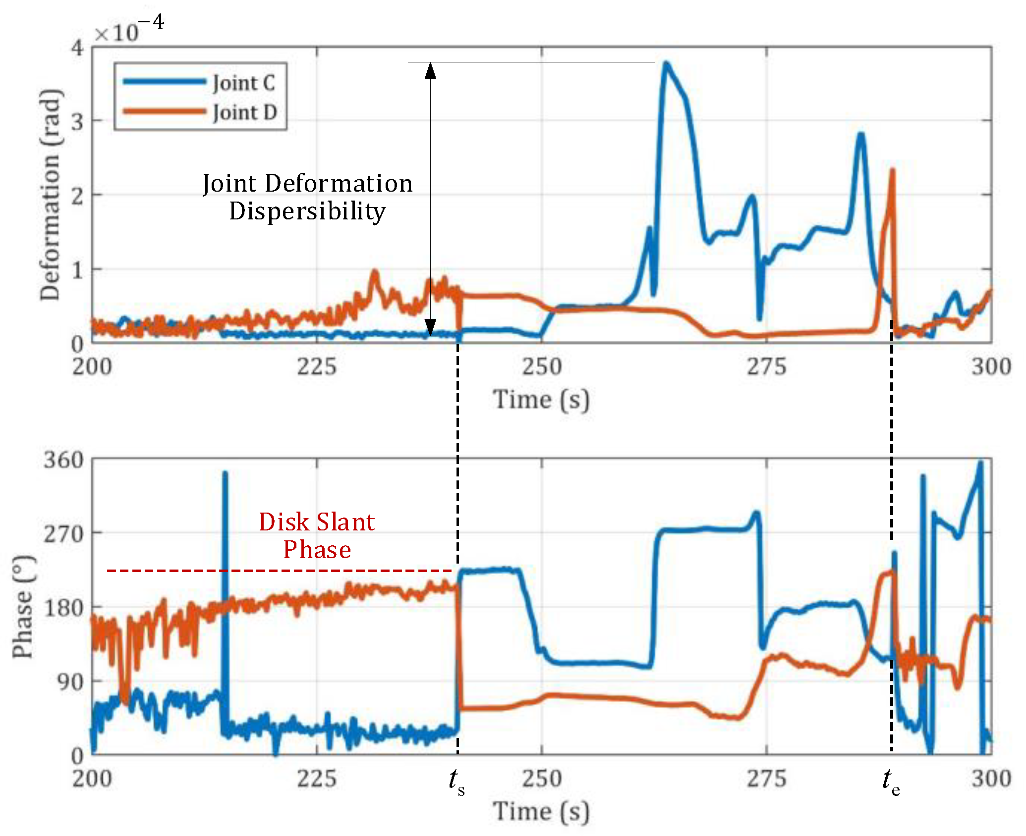
5.2. Rotor Dynamic Response and Joint Angular Deformation

The measurements presented in Figure 19 illustrate the time-varying amplitude and phase of the rotor’s rear bearing load. It is important to note that these measurements were taken when the rotor’s operational speed had significantly exceeded both the first and second critical speeds, and the operational speed continued to rise during the entire data collection interval.
From Figure 19, it is evident that a sudden significant increase in the bearing load occurs at time t s , corresponding to ω = 76 % ω max . As the operational speed continues to increase, the amplitude of the rear bearing load also increases. Notably, despite the rotor speed increasing at a nearly constant rate, with only occasional speed increment pauses, the rate of the bearing load increase exhibits considerable variability. As the operational speed approaches ω = 90 % ω max , a sudden drop in the rear bearing load is observed.
Moreover, an analysis of the rear bearing load phase reveals interesting findings. Prior to the sudden increase in vibration response, the phase of the rear bearing load remains relatively stable around 90°, showing negligible variation with respect to the operational speed. However, during the moment of the sudden increase in vibration response, the phase of the rear bearing load undergoes a rapid shift of approximately 110°. Throughout the vibration-following stage, the phase of the rear bearing load continues to vary, and regions with a higher change rate of the phase align with areas of notable change rate of vibration amplitude.
Time-varying angular deformations for Joint C and Joint D are depicted in Figure 20. It is evident that prior to time t s , the angular deformations at both joints are negligible, and their corresponding phases remain nearly constant. However, at time t s , a small increase in angular deformation is observed at both bolt joints, accompanied by significant changes in the deformation phases. Specifically, the phase of the angular deformation at Joint C aligns closely with the phase change observed in the rear bearing load in Figure 19, confirming that the rear bearing load is attributed to the sudden angular deformation at Joint C. As the operational speed increases, the angular deformation at Joint C continues to vary within [ 0 , 4 ] × 10 4   rad , with multiple phase changes occurring (conversely, the angular deformation of Joint D remains relatively small and can be practically ignored). This indicates that the angular deformation of the bolt joint exhibits non-deterministic behavior due to the discontinuity in the mechanical behavior at the joint interface. Moreover, it is noteworthy that when the angular deformation of Joint C reaches larger magnitudes, the amplitude and phase change rates of the rear bearing load become significantly higher. This is because the larger angular deformation of Joint C results in a larger additional PAI slant of the turbine element, leading to higher rates of variation in the rotor’s dynamic responses with respect to the operational speed.
Obtain α ˜ C ( t ) by experiment data as shown in Figure 20, and substitute α ˜ C ( t ) into Equation (13), and the excitation characteristics of the tested rotor can be corrected. A simulation of the rotor’s dynamic response is then performed based on this distributed excitation. The experimental results, when compared with the theoretical results shown in Figure 21, are in excellent agreement. This provides strong confirmation of the accuracy of the underlying mechanism by which the distributed rotational inertia load excitation model and the sudden angular deformation of the joints influence the rotor’s dynamic response.

6. Conclusions

This paper provides a comprehensive investigation of the high-speed jointed rotor system, with a primary focus on the influence of rotor motion state and joint mechanical characteristics on rotor dynamics. To achieve this, a distributed rotational inertia load excitation model has been developed, which considers both CM offset and PAI slant as forms of mass asymmetry, while also accounting for their axial distribution characteristics. Through simulations and subsequent experimental tests, the dynamic response of the rotor and the factors that significantly influence it have been thoroughly analyzed. The key conclusions derived from this study are as follows:
(1) At high operational speeds, bending deformation compromises the integrity of the rotor, leading to relative angular deformations between mass elements. This results in local mass asymmetry and distributed rotational inertia load excitation, significantly affecting the rotor’s dynamic behavior in the high-speed range.
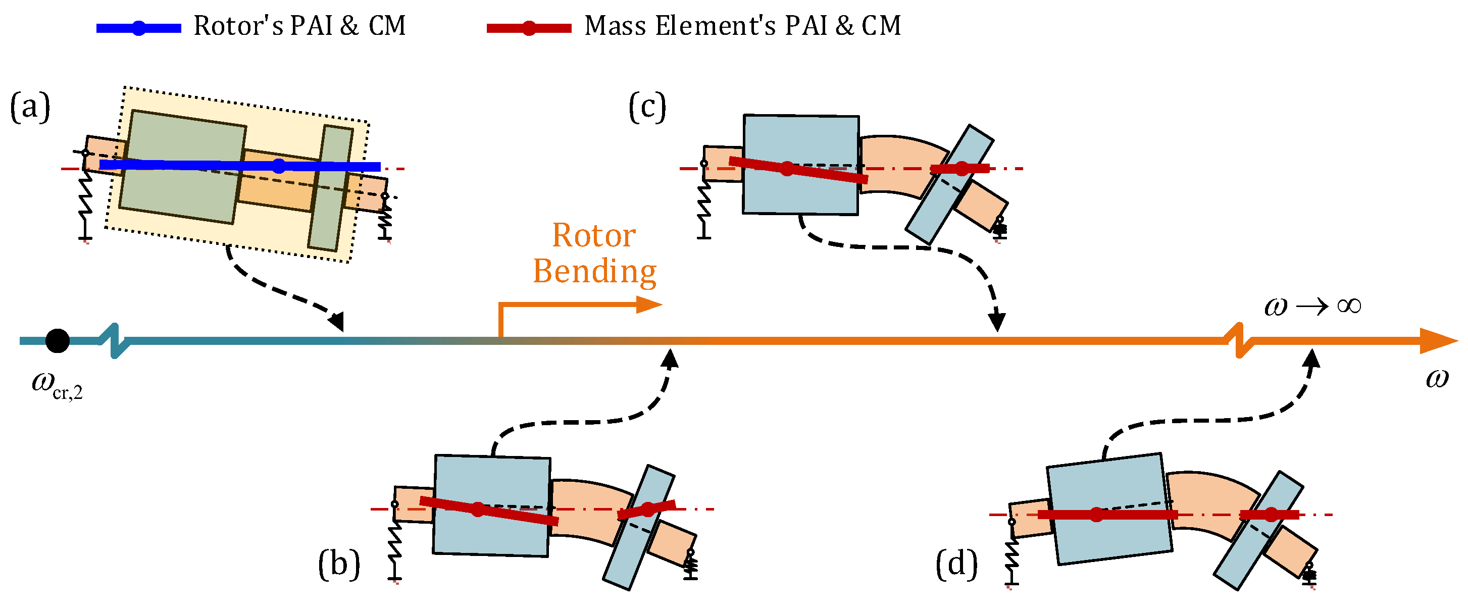
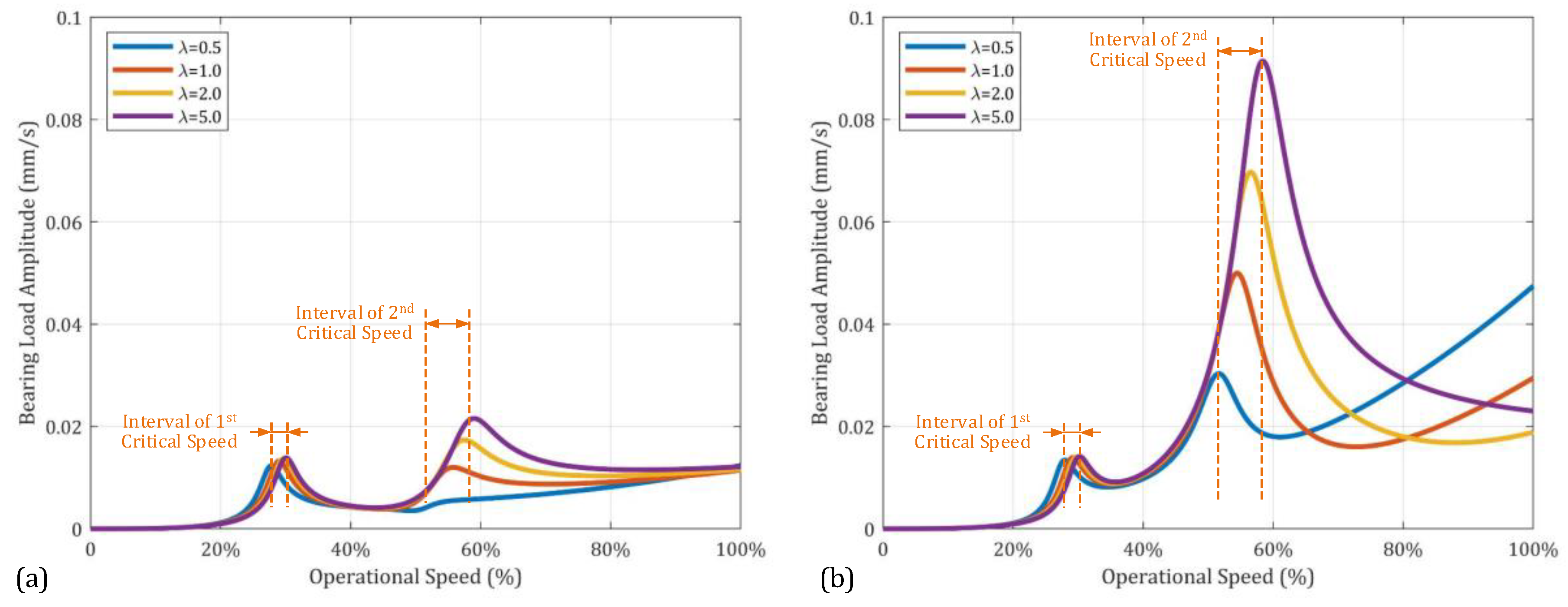
  • In the low-speed range, rotor bending deformation can be neglected, and the rotor can be approximated as a rigid body. The rotor’s CM offset and PAI slant dominate the whole rotor’s dynamic response. However, as the operational speed exceeds the first/second critical speeds, the influence of rotational inertia forces/moments caused by the whole rotor diminishes with increasing speed.
  • In the high-speed range, local mass asymmetry, particularly in the thin-disk turbine element, becomes more evident. The rotational inertia moment generated by the turbine element rapidly increases with the operational speed, even in the supercritical state, becoming the primary excitation source for rotor dynamic response. Excessive PAI slant of the turbine element can lead to a continuous increase and potential over-scale of the rotor’s dynamic response.
(2) Angular deformation of the joints plays a critical role in influencing the rotor mass asymmetry state, leading to changes in rotational inertia load excitation distribution within the rotor and subsequently altering its dynamic response. Considering the discontinuous and uncertain nature of the mechanical characteristics of the joint interfaces under varying loads, the rotor’s dynamic response exhibits significant sudden changes and dispersion features.
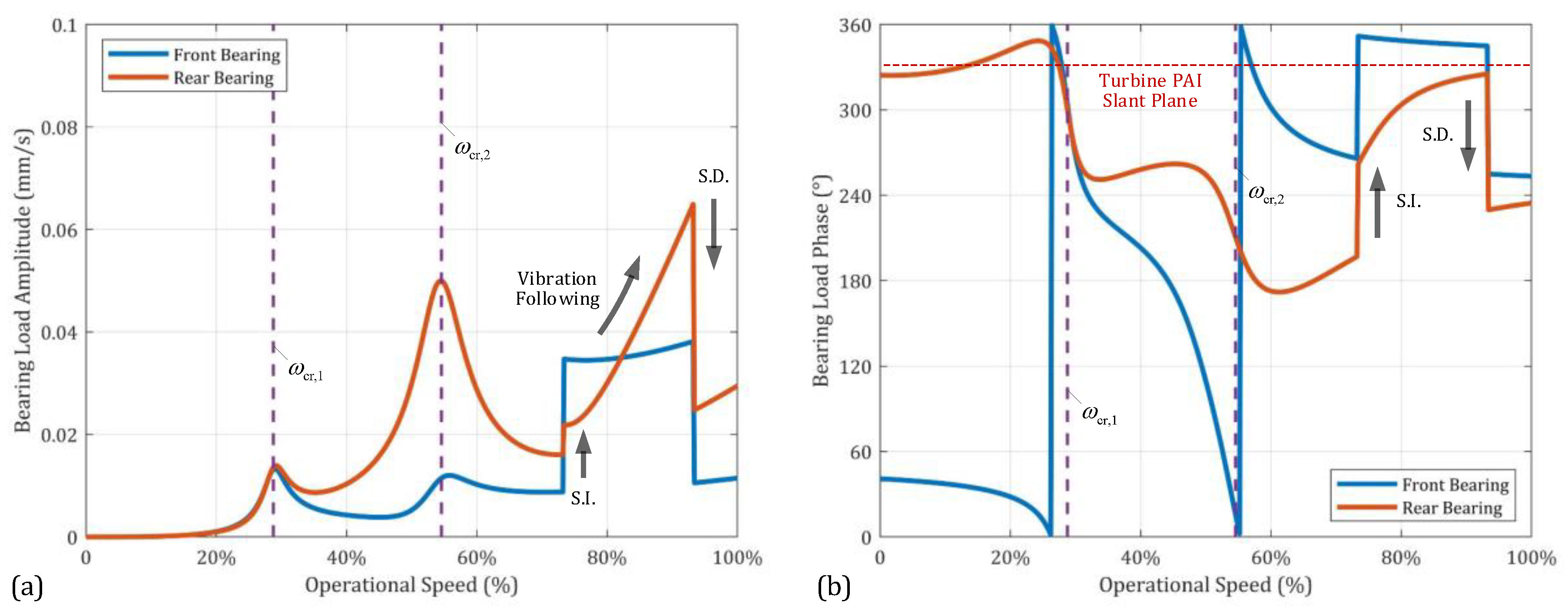
  • Bending stiffness loss in the joints between mass elements weakens the rotor’s integrity, intensifying the effect of the locally generated rotational inertia load and exacerbating the phenomenon of vibration following and dynamic response amplitude at high operational speeds.
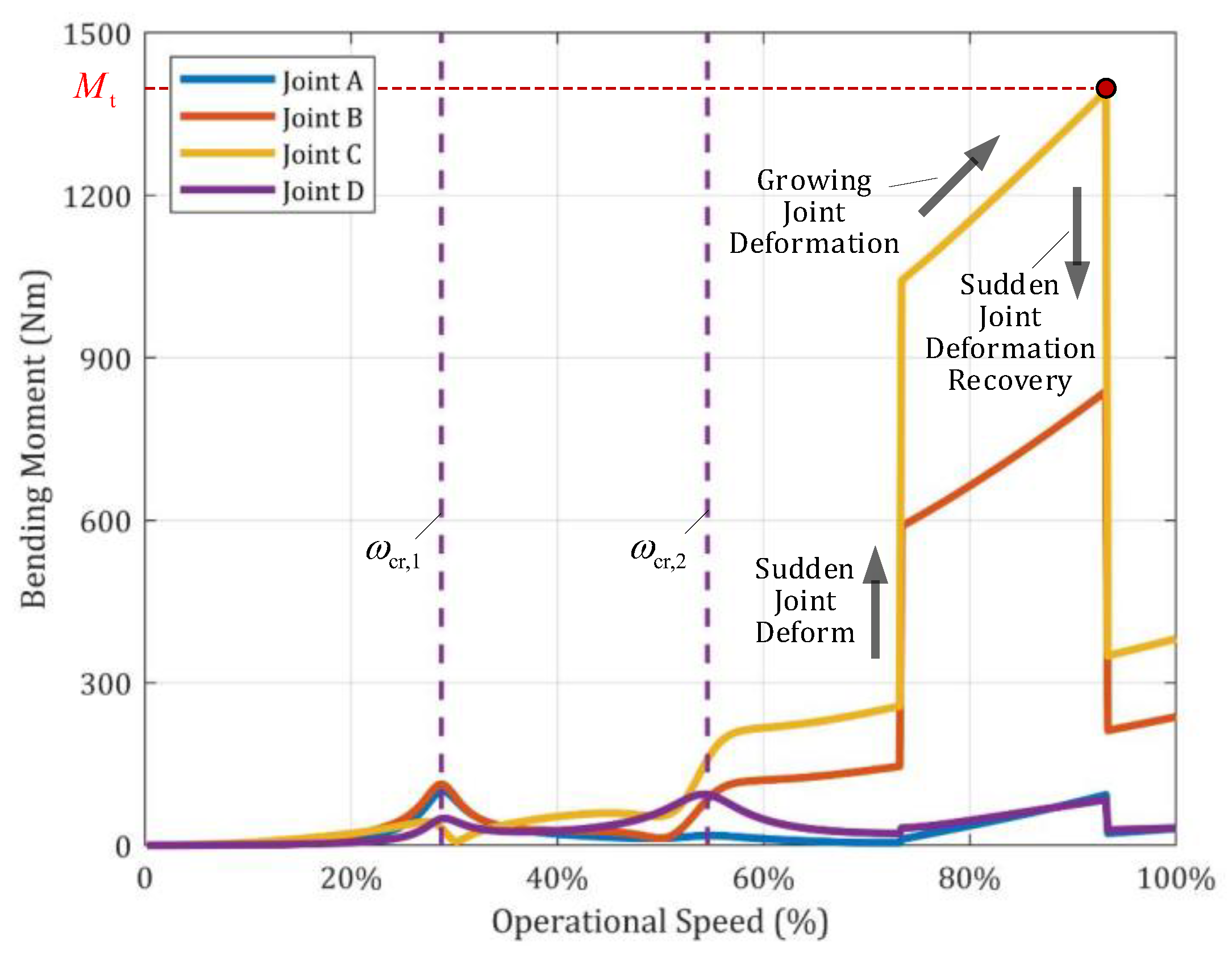
  • Under complex load environments, sudden angular deformation of the joints due to interfacial slip induces a sudden increase in angular displacement of surrounding mass elements, especially for the turbine element. The additional PAI slant of the turbine element causes a sudden increase in rotor dynamic response and vibration following. When the rotational inertia moment is significant enough to cause joint interface slip again, the angular deformation of the joints abruptly decreases, and the PAI of the turbine element returns to its original angular position, leading to a sudden drop in rotor dynamic response.
Nevertheless, the oversimplified representation of inertial and elastic characteristics within the rotor dynamic model may compromise the reliability of the derived rotor dynamic outcomes. Consequently, future research should incorporate more sophisticated mechanical models that duly consider the bending flexibility of shafts and long rotors.

Author Contributions

Conceptualization, F.W.; Software, X.C.; Validation, F.W.; Investigation, F.W.; Resources, F.W.; Data curation, X.C.; Writing—original draft, F.W.; Writing—review & editing, J.H.; Supervision, F.W.; Project administration, X.C. All authors have read and agreed to the published version of the manuscript.

Funding

The authors gratefully acknowledge the financial support provided by the National Science and Technology Major Project (Y2019-VIII-0011-0172) and the Science Center for Gas Turbine Project (P2021-A-I-002-002).

Data Availability Statement

Data is unavailable due to privacy.

Conflicts of Interest

The authors declare that they have no known competing financial interest or personal relationships that could have appeared to influence the work reported in this paper.

References

  1. Jeffcott, H.H. The lateral vibration of loaded shafts in the neighbourhood of a whirling speed—The effect of want of balance. Lond. Edinb. Dublin Philos. Mag. J. Sci. 1919, 37, 304–314. [Google Scholar] [CrossRef]
  2. Rao, J.S. History of Rotating Machinery Dynamics; Springer: New York, NY, USA, 2011. [Google Scholar]
  3. Smith, D.M. The motion of a rotor carried by a flexible shaft in flexible bearings. Proc. Roy. Soc. 1933, 142, 92–118. [Google Scholar]
  4. Den Hartog, J.P. Mechanical Vibrations; McGraw-Hill Book Company: New York, NY, USA, 1940. [Google Scholar]
  5. Timoshenko, S.P. Vibration Problems in Engineering; D. Van Nostrand Company Inc.: New York, NY, USA, 1955. [Google Scholar]
  6. Carnegie, W. Rotary inertia and gyroscopic effects in overhung shaft systems. Bull. Mech. Eng. Educ. 1964, 3, 191. [Google Scholar]
  7. Kikuchi, K. Analysis of unbalance vibration of rotating shaft system with many bearings and disks. Bull. JSME 1970, 13, 864–872. [Google Scholar] [CrossRef]
  8. Cruz, W.; Arzola, N.; Araque, O. Modeling and experimental validation of the vibration in an unbalance multi-stage rotor. J. Mech. Eng. Sci. 2019, 13, 5703–5716. [Google Scholar] [CrossRef]
  9. Datz, J.; Karimi, M.; Marburg, S. Effect of Uncertainty in the Balancing Weights on the Vibration Response of a High-Speed Rotor. J. Vib. Acoust. 2021, 143, 061002. [Google Scholar] [CrossRef]
  10. Lu, Z.Y.; Chen, Y.S.; Li, H.L.; Hou, L. Reversible model-simplifying method for aero-engine rotor systems. J. Aerosp. Power 2016, 31, 57–64. [Google Scholar]
  11. Nicholas, J.C.; Gunter, E.J.; Allaire, P.E. Effect of residual shaft bow on unbalance response and balancing of a single mass flexible rotor—Part I: Unbalance response. J. Eng. Power. 1976, 98, 171–181. [Google Scholar] [CrossRef]
  12. Nicholas, J.C.; Gunter, E.J.; Allaire, P.E. Effect of Residual Shaft Bow on Unbalance Response and Balancing of a Single Mass Flexible Rotor—Part II: Balancing. J. Eng. Power. 1976, 98, 182–187. [Google Scholar] [CrossRef]
  13. Yanhong, M.A.; Haizhou, L.I.U.; Wangqun, D.E.N.G.; Hai, Y.A.N.G.; Jie, H.O.N.G. Vibration response analysis of rotor system with initial thermal deformation. J. Beijing Univ. Aeronaut. Astronaut. 2019, 45, 227–233. [Google Scholar]
  14. Hong, J.; Yan, Q.; Sun, B.; Ma, Y. Vibration Failure Analysis of Multi-Disk High-Speed Rotor Based on Rotary Inertia Load Model. In Proceedings of the Turbo Expo: Power for Land, Sea, and Air, Rotterdam, The Netherlands, 13–17 June 2022; Volume 86076. [Google Scholar]
  15. Ishida, Y.; Toshio, Y. Linear and Nonlinear Rotordynamics: A Modern Treatment with Applications; John Wiley & Sons: Hoboken, NJ, USA, 2013. [Google Scholar]
  16. Liu, Y.; Liu, H.; Wang, N. Effects of typical machining errors on the nonlinear dynamic characteristics of rod-fastened rotor bearing system. J. Vib. Acoust. 2017, 139, 011004. [Google Scholar] [CrossRef]
  17. Han, Z.; Wang, D.; Wang, Y.; Hong, J.; Cheng, R. Dynamic effects of the initial skewness of the inertial principal axis on the rotor with bolted joint. Mech. Syst. Signal Process. 2023, 200, 110564. [Google Scholar] [CrossRef]
  18. Qin, Z.Y.; Han, Q.K.; Chu, F.L. Analytical model of bolted disk-drum joints and its application to dynamic analysis of jointed rotor. Proc. Inst. Mech. Eng. Part C J. Mech. Eng. Sci. 2013, 228, 55808444. [Google Scholar] [CrossRef]
  19. Luan, Y.; Guan, Z.Q.; Cheng, G.D.; Liu, S. A simplified nonlinear dynamic model for the analysis of pipe structures with bolted flange joints. J. Sound Vib. 2012, 331, 325–344. [Google Scholar] [CrossRef]
  20. Zhuo, M.; Yang, L.H.; Yu, L. Contact Stiffness Calculation and Effects on Rotordynamic of Rod Fastened Rotor. In Proceedings of the ASME 2016 International Mechanical Engineering Congress and Exposition, American Society of Mechanical Engineers, Phoenix, AR, USA, 11–17 November 2016. [Google Scholar]
  21. Hong, J.; Chen, X.; Wang, Y.; Ma, Y. Optimization of dynamics of non-continuous rotor based on model of rotor stiffness. Mech. Syst. Signal Process. 2019, 131, 166–182. [Google Scholar] [CrossRef]
  22. Ma, Y.; Ni, Y.; Chen, X. Bending stiffness loss of rod-rabbet joints and its effect on vibration response of rotor systems. Acta Aeronaut. Astronaut. Sin. 2021, 42, 223861. [Google Scholar]
  23. Chen, X.; Ma, Y.; Hong, J. Vibration suppression of additional unbalance caused by the non-continuous characteristics of a typical aero-engine rotor. In International Conference on Rotor Dynamics; Springer: New York, NY, USA, 2018; pp. 34–48. [Google Scholar]
  24. Liu, S.; Ma, Y.; Zhang, D.; Hong, J. Studies on dynamic characteristics of the joint in the aero-engine rotor system. Mech. Syst. Signal Process. 2012, 29, 120–136. [Google Scholar] [CrossRef]
  25. Liu, Y.; Liu, H.; Fan, B.W. Nonlinear dynamic properties of disk-bolt rotor with interfacial cutting faults on assembly surfaces. J. Vib. Control 2018, 24, 4369–4382. [Google Scholar] [CrossRef]
  26. Liu, Y.; Liu, H.; Fan, B. Numerical analysis on the static–dynamic coupling influences of parallelism flaw in disc-rod rotor ball bearing system. Proc. Inst. Mech. Eng. Part K J. Multi-Body Dyn. 2018, 232, 103–112. [Google Scholar] [CrossRef]
  27. Barragan, J.M. Engine Vibration Monitoring and Diagnosis Based on On-Board Captured Data; MTU Aero Engines Gmbh Munich: Munich, Germany, 2003. [Google Scholar]
  28. Zhao, B.; Sun, Q.; Zhao, R.; Yang, Y.; Sun, K.; Mu, X. Mass-eccentricity nonlinear evolution mechanism of combined rotor in fretting slip process. Tribol. Int. 2023, 179, 108195. [Google Scholar] [CrossRef]
  29. Zhao, B.; Sun, Q.; Yang, Y.; Sun, K.; Liu, Z. Study on interface non-uniform slip of combined rotor considering real preload distribution. Tribol. Int. 2022, 169, 107482. [Google Scholar] [CrossRef]
  30. Wang, C.; Zhang, D.; Zhu, X.; Hong, J. Study on the stiffness loss and the dynamic influence on rotor system of the bolted flange joint. In Proceedings of the Turbo Expo: Power for Land, Sea, and Air, Dusseldorf, Germany, 16–20 June 2014; Volume 45769. [Google Scholar]
  31. Nizametdinov, F.R.; Romashin, Y.S.; Berne, A.L.; Leontyev, M.K. Investigation of bending stiffness of gas turbine engine rotor flanged connection. J. Mech. 2020, 36, 729–736. [Google Scholar] [CrossRef]
  32. Hong, J.; Xu, X.; Su, Z.; Ma, Y. Joint stiffness loss and vibration characteristics of high-speed rotor. J. Beijing Univ. Aeronaut. Astronaut. 2019, 45, 18–25. [Google Scholar]
Figure 1. A typical high-speed jointed rotor: P1—front shaft element; P2—compressor element; P3—drum shaft element; P4—turbine element; P5—rear shaft element.
Symmetry 15 02009 g001
Figure 2. Mass asymmetry of an element and its description method: (a) body-fixed translation coordinate system of the element, referred to as x 1 M y 1 . This coordinate system has the element’s centroid M as its origin, and its coordinate axes align with the absolute coordinate system. In this coordinate system, G —the element’s CM, I p , I d —the element’s PAI, ω x 0 , ω y 0 , ω z 0 —components of rotor’s rotation ω in the direction of the element’s PAI; (b) mass center coordinate system of the element, referred to as x 0 G y 0 . This coordinate system has the element’s CM G as its origin, and the line of intersection between planes x 1 M y 1 and x 0 G y 0 as x -axis. In this coordinate system, i , k —directions vector of x -axis and z -axis, respectively. e —distance between the element’s CM and centroid, τ —angle between the PAI and the rotor’s rotation axis, L x 0 , L y 0 , L z 0 —components of the element’s angular momentum along the x , y , z axes of coordinate x 1 M y 1 . (c) The projection of the element’s PAI slant and CM offset onto plane x 1 M y 1 , where β e , β τ —phase of the CM offset and PAI slant.
Symmetry 15 02009 g002
Figure 3. Axial distribution and representation of mass asymmetry in high-speed rotors: m i —mass of the i th element; I p , i , I d , i —polar and diametral moment of inertia of the i th element; τ ˜ i —angles between the i th element’s PAI and the centroid line of this element, e ˜ i —distance between the i th element’s CM and the centroid line of this element.
Symmetry 15 02009 g003
Figure 4. Variation of a rotor’s motion with the operational speed (low-speed range): (a) while rotating at low speed, the rotor can be regarded as a thick-disk, where, m r , I p , r , I d , r —mass and moment of inertia of the rotor, e ˜ r , τ ˜ r —CM offset and PAI slant of the rotor, ω —operational speed; (b) the rotational inertia force generated by the CM offset increases with the rotational speed, enhancing the rotor’s lateral displacement; (c) when ω exceeds the first critical speed ω cr , 1 , the rotor undergoes the turning inward of CM; (d) the rotor’s CM gradually approaches the rotor’s rotation axis, resulting in a gradual decrease in the rotational inertia force. However, the rotational inertia moment produced by the rotor’s PAI slant increases rapidly with the operational speed, enhancing the rotor’s angular displacement; (e) as ω surpasses the second critical speed ω cr , 2 , the rotor’s PAI changes direction; (f) the rotor’s PAI gradually approaches the rotor’s rotation axis, leading to a gradual reduction in the rotational inertia moment and a consequent decrease in the angular displacement of the rotor.
Symmetry 15 02009 g004
Figure 5. Variation of a rotor’s motion with the operational speed (high-speed range): (a) the CM and PAI of the rotor are nearly aligned with the rotation axis; (b) with increasing ω , the rotor undergoes bending deformation, leading to the disruption of the structural integrity of the rotor. At this stage, it becomes necessary to separately consider the mass asymmetry and motion states of the compressor and turbine element; (c) due to the thin-disk characteristic of the turbine element, the rotational inertia moment generated by this element becomes more pronounced compared to the compressor element as ω increases. Consequently, the PAI of the turbine element aligns with the rotation axis first, and the angular displacement of the turbine element no longer increases with further operational speed increase; (d) upon reaching sufficiently high operational speed, the rotational inertia load induced by the compressor element also increases to the point where its PAI aligns with the rotation axis. After this threshold, the angular displacement of the compressor element ceases to increase with further operational speed increments.
Symmetry 15 02009 g005
Figure 6. Influence of a joint’s bend stiffness loss on the distribution of rotational inertia load in a rotor at high operational speed: (a) while the bending stiffness of Joint C, denoted as k J , C is greater than that of Joint D, denoted as k J , D . In the diagram, F ˜ b , f , F ˜ b , r —bearing load at the front and rear bearing, respectively, M ˜ g , r —rotational inertia moment generated by the rotor; (b) when k J , C < k J , D . In the diagram M ˜ g , 2 , M ˜ g , 4 —local rotational inertia moment generated by the compressor element and turbine element, respectively.
Symmetry 15 02009 g006
Figure 7. Influence of angular deformation of the joints on the slant of an adjacent mass element’s PAI: (a) in the initial state, the slant of the PAI of the mass element is τ ˜ ; (b) due to the local angular deformation α ˜ of the joint near this mass element, its PAI undergoes an additional slant, resulting in an equivalent slant angle τ ˜ = τ ˜ + α ˜ .
Symmetry 15 02009 g007
Figure 8. Structural and mechanical parameters of the rotor and its elements: (a) for the i th element, m i -mass, I p , i , I d , i —polar moment of inertia and diametral moment of inertia, k θ , i —bending stiffness, z ˜ i , θ ˜ i —lateral displacement and angular displacement of the element’s CM, l i —axial length, l m , i —axial distance between the front end face of the element and its CM. k bf , k br , c bf , c br —stiffness and damping coefficient of the front and rear bearing, k J , i —bending stiffness of the i th joint; (b) during rotor dynamic analysis, only the rotational inertia load excitations caused by the CM offset and the PAI slant of the mass elements are considered.
Symmetry 15 02009 g008
Figure 9. Equivalent method for the influence of joints’ bending stiffness loss on rotor stiffness. In this method, based on the assumption of constant section beams, the bending stiffness between the i th and ( i + 1 ) th elements’ angular DoF is obtained by serially connecting the joint and its adjacent components.
Symmetry 15 02009 g009
Figure 10. Process of the effect of joints’ angular deformation on the dynamic characteristics of a high-speed rotor: (a) in low-speed ranges, since the initial PAI slant τ ˜ is relatively small and the operational speed ω is low, the rotational inertia load generated by the elements during operation and the resulting rotor bending deformation can be negligible; (b) when ω increases to ω t , the loads applied to the joint cause their interfaces to slip, resulting in sudden angular deformation α ˜ of the joint. This leads to the turbine element’s slant and corresponding rotational inertia moment M ˜ g . This M ˜ g not only acts back on the joint, causing it to experience bending moment M ˜ J , but also induces bearing loads F ˜ b at the rear bearing; (c) as ω continues to increase, M ˜ g increases rapidly, and the bending deformation of the adjacent elastic elements intensifies accordingly. Consequently, as the rear bearing acts as a constraint boundary, in order to balance the bending deformation within the elastic elements, the bearing loads F ˜ b also increase rapidly with ω ; (d) when M ˜ J exceeds a certain threshold, the joint undergoes a sudden angular deformation change, with residual angular deformation α ˜ r , causing a sudden decrease in the angle between the element’s PAI and the rotor’s rotation axis. Simultaneously, as the rotational inertia moment generated by the turbine element decreases, the bending deformation of the elastic elements and the resulting bearing reaction force also experience a sudden drop.
Symmetry 15 02009 g010
Figure 11. Rotor’s dynamic response under different rotational inertia load excitation models: (a) amplitude of front and rear bearing loads. ω cr , 1 , ω cr , 2 —first/second critical speed of the rotor; (b) phase of front and rear bearing loads.
Symmetry 15 02009 g011
Figure 12. Rotor mass elements’ angular displacement under different rotational inertia load excitation models: (a) amplitude of mass element’s angular displacement; (b) phase of mass element’s angular displacement.
Symmetry 15 02009 g012
Figure 13. Impact of joints’ bending stiffness on bearing load: (a) amplitude of front bearing load at different joints’ bending stiffness, where λ represents the ratio of the bending stiffnesses of the front and rear bolt joints of the turbine element; (b) amplitude of rear bearing load at different joints’ bending stiffness.
Symmetry 15 02009 g013
Figure 14. Impact of rotational inertia load excitation model and joints’ bending stiffness on rotor dynamics.
Symmetry 15 02009 g014
Figure 15. Rotor dynamic response characteristics considering the joint’s sudden angular deformation: (a) amplitude of bearing load; (b) phase of bearing load.
Symmetry 15 02009 g015
Figure 16. Variation of the bending moment applied to the joints of a high-speed rotor with the operational speed.
Symmetry 15 02009 g016
Figure 17. Variation of rotor mass elements’ angular displacement with the operational speed considering joints’ sudden angular deformation: (a) angular displacement amplitude of the mass elements; (b) angular displacement phase of the mass elements.
Symmetry 15 02009 g017
Figure 18. High-speed jointed rotor dynamic characteristics test rig: displacement sensors D 3 1 , D 3 2 are used to measure the lateral displacement at two sections of the drum shaft element, with an axial distance of L 3 between the two sections. Each section is equipped with two displacement sensors to measure the horizontal/vertical displacement of the rotor at that position. Displacement sensors D 4 , D 5 are used to measure the axial displacement of the turbine element and the rear shaft element, at distances L 4 , L 5 from their respective centroid axes. Each element is equipped with two sensors to measure its axial displacement in the horizontal and vertical planes.
Symmetry 15 02009 g018
Figure 19. 1× RPM component of the rotor rear bearing load: the top graph shows the rotor operational speed, the middle graph shows the amplitude of the rear bearing load, and the bottom graph shows the phase of the rear bearing load. Here, t s , t e —the starting and ending moments of the rotor’s abnormal vibration.
Symmetry 15 02009 g019
Figure 20. Rotor joints’ angular deformation: the top graph shows the amplitude of the joints’ angular deformation, and the bottom graph represents the phase of the joints’ angular deformation.
Symmetry 15 02009 g020
Figure 21. Comparison between experimental results and theoretical results.
Symmetry 15 02009 g021
Table 1. Mass/moment of inertia/bending stiffness of the rotor and its elements.
Element IDP1P2P3P4P5Rotor
m (kg)101001010010230
I p ( kg mm 2 )7.0 × 1043.5 × 1061.5 × 1055.5 × 1061.5 × 1059.4 × 106
I d ( kg mm 2 )7.8 × 1054.7 × 1061.2 × 1052.8 × 1068.3 × 1042.8 × 107
I p / I d 0.090.741.261.941.800.33
k θ ( N m / rad )7.3 × 10910.0 × 10102.6 × 10910.0 × 10100.4 × 109-
Disclaimer/Publisher’s Note: The statements, opinions and data contained in all publications are solely those of the individual author(s) and contributor(s) and not of MDPI and/or the editor(s). MDPI and/or the editor(s) disclaim responsibility for any injury to people or property resulting from any ideas, methods, instructions or products referred to in the content.

