Article

Elastic Wave Mechanics in Damaged Metallic Plates

by
Samuel Chukwuemeka Olisa
,
Muhammad A. Khan
* and
Andrew Starr
Centre of Life-Cycle Engineering and Management, Cranfield University, Cranfield MK43 0AL, UK
*
Author to whom correspondence should be addressed.
Symmetry 2023, 15(11), 1989; https://doi.org/10.3390/sym15111989
Submission received: 3 October 2023 / Revised: 20 October 2023 / Accepted: 25 October 2023 / Published: 27 October 2023
(This article belongs to the Special Issue Advances in Structural Mechanics and Symmetry/Asymmetry)

Abstract

:
Human health monitoring (HHM) is essential for continued daily task execution, as is structural health monitoring (SHM) for structures to ensure the continual performance of their designed tasks with optimal efficiency. The existence of damage in a structure affects its optimal use through stiffness deterioration. Damage of different forms could occur in a structure but have the singular objective of material degradation, leading to its underuse for a task. Guided wave ultrasonics has shown strength in detecting sundry damage in structures, but most of the damage monitored and detected is unfilled with substances. However, some damage could trap and accumulate substances that could hasten material degradation through corrosion activities under favorable conditions, especially in the oil and gas industry. This study used the ultrasonic-guided waves’ pitch–catch inspection technique to identify damage filled with different materials. The assessment was based on the RMSD of the dominant Lamb wave mode’s average maximum amplitude and the response signals’ transmission coefficient (TC). A five-cycle tone burst of excitation signals of different frequencies was created to generate propagating Lamb waves in the structure. The fundamental antisymmetric mode was found to be more sensitive than the fundamental symmetric mode when detecting damage filled with various substances. At 80 kHz, the deviation of the current response signals from the baseline response signals due to different filled substances in the damage was distinct and decreased with increased fluid viscosity. Given that structures in the oil and gas sector are particularly susceptible to substance-induced damage, the outcomes of this study are paramount.

1. Introduction

Engineering structures are often constructed using materials that ensure a long service life for an intended task. The metal plate is the base of most civil engineering structures. Some essential economic structures are formed and constructed using thin or thick plates. One of the ways to classify a plate as thin or thick is through the ratio of its thickness to other geometric dimensions [1]. If the plate’s thickness is greater than one-tenth of its other geometric dimensions, it is called a thin plate; otherwise, it is a thick plate as defined in the piecewise function of Equation (1).
f D =         t h i n p l a t e ,     i f         D = T W / L < < 0.1 t h i c k p l a t e ,     i f       D = T W / L > 0.1
where D is the ratio between the plate thickness (T) and either the width (W) or length (L) of the plate. The thickness of a structure is essential to supporting and carrying loads designed for it. Variation in the thickness of a structure leads to a hotspot for material degradation and a high chance for catastrophic failure. Structural damage that causes thickness variation has been associated with corrosion activities [2]. The initiation of corrosion activities in different ways is revealed in [3]. Early damage detection is necessitated due to the severe implications of damage to structures, especially during service time. Undetected damage could lead to a failure of the structure, which may cost lives and high-valued economic assets used in the aviation sector and the oil and gas industry.
Structural health monitoring (SHM) was devised for the continuous monitoring of structures using different techniques to detect and estimate characteristics of damage in the structure [4,5,6,7]. Different authors have used vibrational responses to detect damage in structures, but this technique is suitable primarily for dynamic structures and propagating cracks [8,9,10,11]. In the past decade, interest in using guided wave ultrasonic technique (GWUT) to monitor thin structures has increased tremendously due to its cost-effectiveness, long-distance inspection capability, nonintrusive nature and light weight [12]. Using the GWUT configuration, Lamb waves can be generated to travel through the thickness of structures. These waves gather data from specific areas of the structure by interacting with them and are recorded as response signals of the structures by a sensor. Pulse–echo (P–E) and pitch–catch (P–C) configurations are primarily used for this purpose, with emphasis on the nature and size of the damage. P–E is principally used to monitor large damage in structures that could reflect most incident waves when encountered. However, P–C is ideal for small damage sizes, such as corrosion damage, because it allows for the through-transmission of the incident wave with little reflection [12]. Unlike P–E, P–C detects damage in the area between the exciter and the sensor. Damage in structures can be empty or filled with substances, given that nature abhors a vacuum. Damage filled with substances could be dominantly found in static structures. Substances in this study are referred to as debris or fluid [3]. Empty damage is formed when a crack, dent or notch is devoid of filled substances, while filled damage is formed when the damage traps and accumulates debris or fluid that could close it. The filled damage has the potential for pitting corrosion formation over time [3]. Pitting corrosion is a localized damage with various depths and irregular geometry. It has been attributed to catastrophic structural failure, especially in the oil and gas industry [13]. Many studies have been performed in detecting unfilled damage, with limited studies on detecting filled damage using GWUT. In [14], the authors studied the relationship between the scattering of damage signals and different severities of damage using the S 0 Lamb wave mode of the pitch–catch method. The severities considered were notch length, orientation and notion depth with respect to the plate thickness. In [15], the authors developed a novel method to detect and estimate crack sizes in metallic plates using guided wave propagation. It was found that wave amplitude, influenced by damage interactions, varied notably based on crack location. In [16], crack severity due to damage depth variation by uniform incremental percentage was studied using guided wave ultrasonics and different damage indices. In [17], the authors explored structural health monitoring using ultrasonic-guided waves in complex structures, specifically plates with stiffeners. The research inferred crack size and shape from the wave patterns by comparing them with a crack-free benchmark. The RMSD was noted to be more reliable than other DI metrics. Delamination, corrosion and debonding have also been studied using ultrasonic-guided waves [12]. Nevertheless, there are limited studies on the detection of filled damage, especially when the damage was filled with either dry debris or fluids. In this research, the detection of filled damage was experimentally investigated using GWUT through the pitch–catch technique with three sensors and an exciter. Varying substances were used to fill the damage; each is called a state of the damage. The deviation of each damage state response from the healthy state at every excitation frequency was computed using root mean square deviation (RMSD). Similarly, the transmission coefficient (TC) of the response signals due to varying damage states was also examined. Through the dispersion curve, relatively stable excitation frequencies were selected to ensure the generation of only fundamental modes. This study was performed on a plate of a 3.00   m m thickness with a seeded damage of a 2.50   m m depth. Three case scenarios were studied: (a) a base case using a healthy plate; (b) an unhealthy plate using empty damage; and (c) filled-in damage with different substances. The respective influence of each substance on the guided wave on predicting damage was observed and compared with the healthy state.

2. Theory of Lamb Wave Generation and Propagation in Thin Structures

2.1. Nondestructive Evaluation Technique

Elastic waves are vital for damage detection and severity evaluation in structural health monitoring (SHM). Such waves occur through restoration forces between particles of the host structure temporarily displaced from their mean positions. The excitation of the elastic waves in structures causes changes in the material properties and thereby influences the characteristics of the propagating wave, such as the wavelength, time of wave arrival (ToA), time of flight (ToF) and amplitude. Elastic waves can be bulk waves or guided waves [18]. The two forms of elastic waves differ in some respects, although they obey the same governing equations, especially in their mode formation and interactions with the boundaries of the structure [19]. The bulk waves generate finite wave modes while propagating within the material but away from its boundaries. The boundaries of the structure guide the guided wave, in contrast to the bulk wave. Due to the dispersive nature of the guided wave through wave velocity dependence on frequency, multiple modes are generated, leading to complexity in wave interpretation. Prominent forms of guided waves are Lamb waves and Rayleigh waves [20]. The Lamb wave can be generated from the coupling between longitudinal and vertical shear waves reflected at the free surfaces of a structure, especially the plate, while Rayleigh waves are free waves on the surface of a semi-infinite solid. In this form of the guided wave, the traction forces vanish on the structure’s surface, and the wave amplitude decays into the depth of the structure. However, the Lamb wave’s traction forces vanish on the guided wave’s upper and lower surfaces as it propagates through the structure’s thickness.
Rayleigh waves are useful in detecting damage in thick structures, while Lamb waves are useful in detecting damage in thin structures [21]. Structures can be monitored in two ways: actively or passively [20]. In the active monitoring technique, a transducer is used as an exciter to cause the propagation of an elastic wave in the structure. At the same time, the structural response is captured by another transducer functioning as a sensor. Unlike the active monitoring technique, the passive monitoring technique offers only listening to emitted response signals generated by the damage [22]. This approach is mainly used to infer the state of the structure because the damage can emit elastic waves in the frequency range of an ultrasound [12]. Hence, as the damage of interest could hardly generate stress waves for its detection, an active monitoring approach was suitable for this study and thereby adopted.

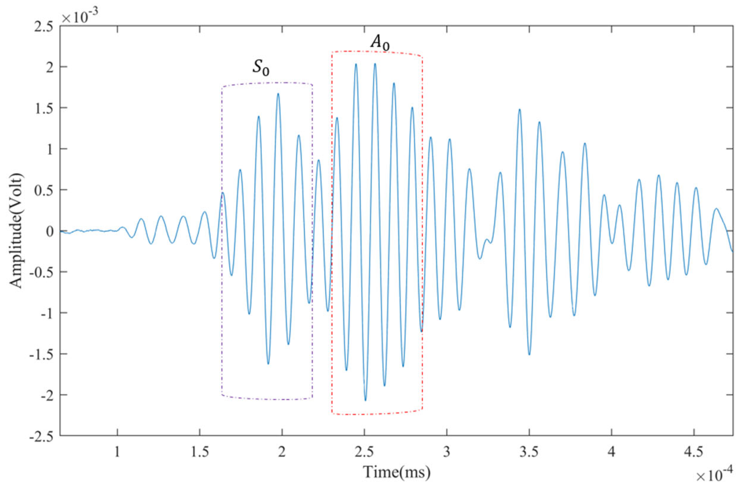
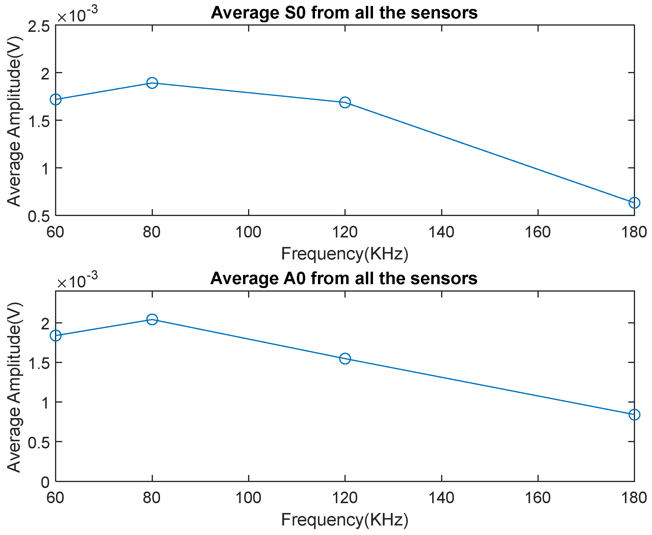
2.2. Directivity and Attenuation of the Lamb Wave

Lamb waves that are excited within structures show changes in some characteristic parameters after encountering damage compared to before. Propagating Lamb waves are captured as a response signal of the structure to the exerted stress wave by the exciter. In the healthy state of a structure and devoid of environmental effects, the intensity of the response signal would be approximately consistent in magnitude. Still, it would vary with the wave propagation path and location of the sensor [23]. Without damage, a sensor in a direct path with an exciter would receive much of the propagated signals, especially when the distance apart was small compared to sensors installed in other paths of the structure, but at the expense of the crosstalk effect. However, structures in service are highly prone to sustaining damage of varying types and degrees of severity. Figure 1 represents the fundamental Lamb wave modes propagating under a structure’s healthy and damaged conditions. It shows that S 0 propagates faster than A 0 but A 0 is the dominant mode.
In Figure 1, the wave’s interaction with the damage led to distinct effects observed in the two wave modes. Among the observed effects were reflected waves, labelled as R waves, waves scattered or deflected by the damage tips, indicated as Des waves, and attenuated through-transmitted waves, represented by a Tt wave. In the pulse–echo inspection configuration, the reflected wave created a new packet. However, in the pitch–catch inspection configuration, the wave’s attenuation effect was more evident [24]. Although the edge of the structure could cause similar reflections, its arrival time would be different from the new packet wave created by the reflection from the damage and the same with the intensity of both effects. In the study, a wave absorber was placed at the edges of the plate to reduce the edge reflection wave. The intensity of the new packets due to wave–damage interaction in P–E suggests the severity of the damage encountered. Based on the damage’s size, some incident waves will pass through, while the damage will reflect others. The edge of the damage also plays a role in the signal’s edge scattering. This study assessed the influence of debris-filled damage and damage filled with different fluids. Three sensors were set up to detect both through-transmitted and edge-reflected waves. The recorded responses underwent processing and analysis to predict the structure’s damage condition.

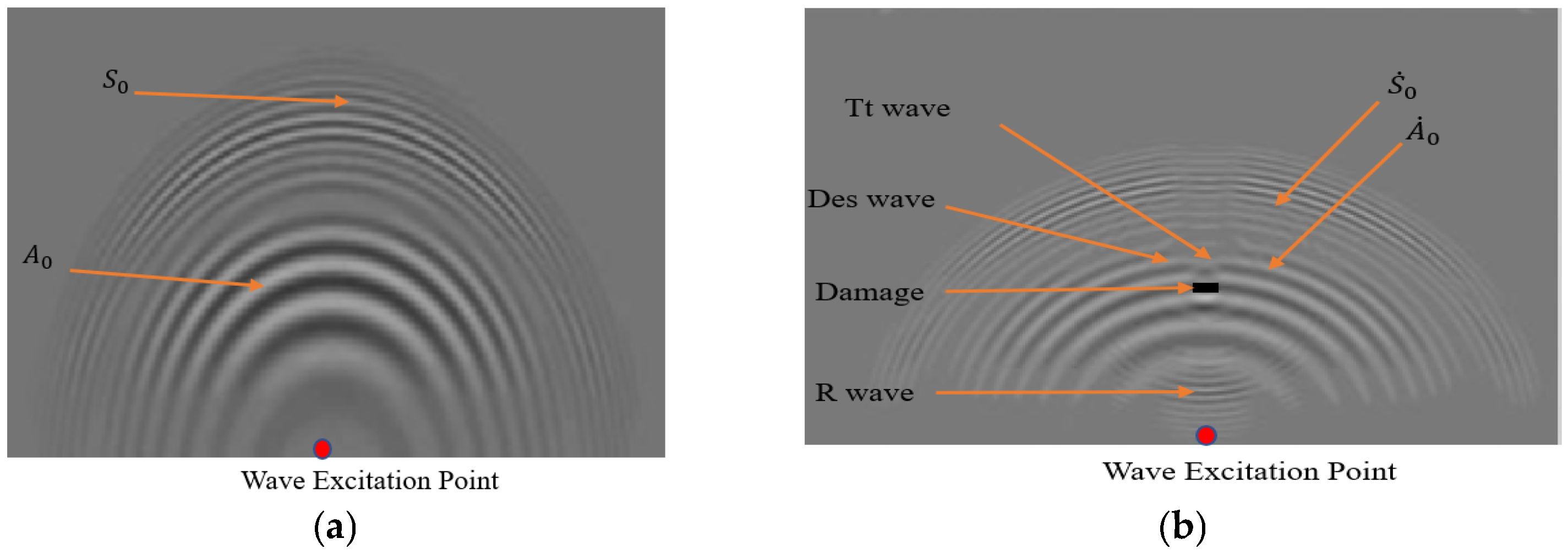
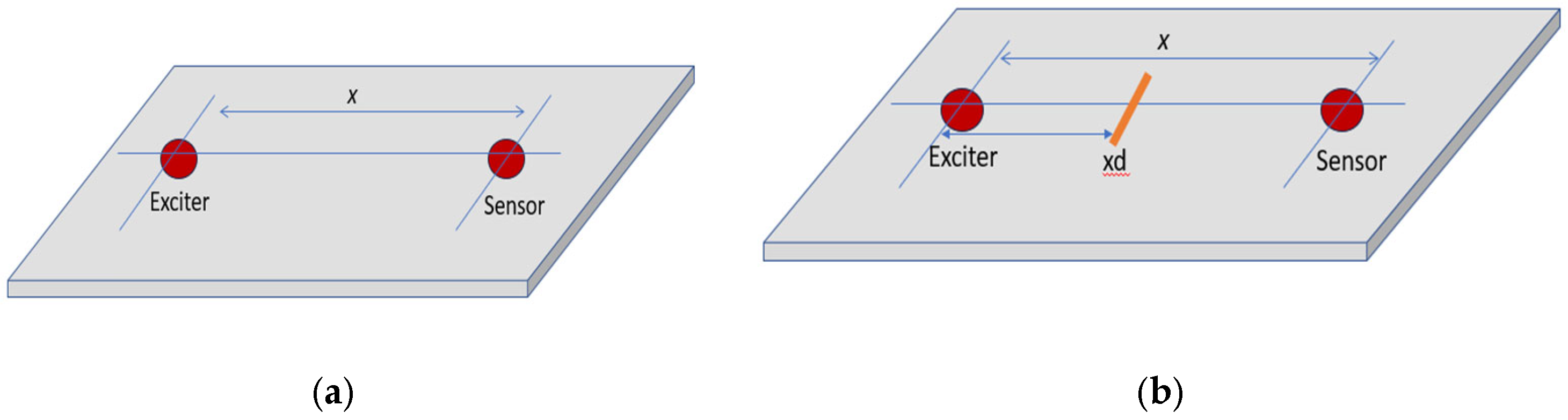
2.3. Modelling Damage Detection Evaluation

Consider an active pitch–catch inspection method in Figure 2. Figure 2a is the healthy case, while Figure 2b is the unhealthy case. The model consists of an exciter, a thin plate and a sensor. The exciter and sensor are of the same type and size. They are coupled to the thin plate using a thin-layer adhesive bond and separated by a distance x . The thickness of the adhesive layer is smaller than the thickness of the transducers but strong enough to keep bonding the transducers to the thin plate. When a sinusoidal electrical signal is applied to the exciter, it creates a surface shear stress around the exciter, resulting in Lamb wave propagation through the thin plate’s thickness. The propagating waves interact with the thin plate and become captured by the sensor at x . Consider such bonding between the transducers and the structure to be ideal. Also, reflection from boundary edges is considered negligible within the duration of Lamb wave propagation and wave capturing at the sensor position, x
Let the electrical signal applied to the exciter be as in Equation (2):
V e ( t ) = V 0 e i ω t
Taking the FFT of Equation (2) would result in Equation (3):
V e ´ ω = t 1 t 2 f ( V e ) e x d t
Under the healthy conditions of the plate and propagation of only fundamental Lamb wave modes, the final received response signal at the sensor position in the frequency domain is as given in Equation (4):
V r x , ω = S 0 ( ω ) V e ´ ( ω ) e i k S 0 x + A 0 ( ω ) V e ´ ( ω ) e i k A 0 x
Similarly, under unhealthy conditions, as in Figure 2b, the captured response signal in the frequency domain is as given in Equation (5):
V r x ´ ( ( x x d ) , ω ) = S 0 ( ω ) V e ´ ( ω ) e i k S 0 ( x x d ) + A 0 ( ω ) V e ´ ( ω ) e i k A 0 ( x x d )
where S 0 ( ω ) and A 0 ( ω ) serve as modal participation functions, dictating the amplitude of the captured fundamental symmetric and antisymmetric wave modes [25].
By applying FFT to Equations (4) and (5), the time–domain response of the captured response signals is as expressed in Equations (6) and (7), respectively.
    V r x , t = IFFT V r x , ω
V r x x x d , t = IFFT V r x ´ x x d , ω
The health condition of the thin plate can be ascertained by comparing Equation (6) and Equation (7) and assessing either mode through its prevalent sensitive signature or maximum peak energy. Thus, the change in the structural response signals resulting from different damage states is calculated using the statistical root mean square difference (RMSD) as described in Equation (8):
R M S D = i = 1 n   A V A i D A V A i P 2 i = 1 n   A V A i P 2
in which A V A i D represents the average maximum amplitude of either the fundamental symmetric or antisymmetric mode from the response signal of a damaged plate and A V A i p denotes the average maximum amplitude from the response signals of a pristine plate. The average maximum peak of any of the modes can be deduced using Equation (9):
A V A z i z 0 = 1 N f j m a x _ p e a k z i z 0
m a x _ p e a k z i z 0 = max ( t 1 T t 2 u ( t ) )
where N is the number of sensors, f j denotes a given frequency of the excitation signal and z i z 0 denotes the fundamental symmetric or antisymmetric mode of any of the sensors where i = 1 ,   2   o r   3 is the sensor number.

2.4. Transmission Coefficient (TC)

When propagating guided waves encounter damage in a structure, they will scatter, resulting in certain phenomenal effects. Among these effects are wave mode conversion, loss of energy, attenuation and reflection as discussed in Section 2.2. Depending on the nature and geometrical variation in the damage, any of the effects could be well pronounced. Also, wave scattering depends on the characteristics of the propagating guided wave as shown in the discussed formed wave equations above. The chances of detecting damage in a structure rely on the characteristics of the propagating wave and damage geometrical parameters, which could be size of the damage, orientation of the damage or nature of the damage. The nature of damage implies filled and unfilled damage. The nature of damage, especially filled damage, contributes more to the phenomena of wave attenuation or energy loss or variation in transmitted signal power distribution after wave–damage interaction. The transmission coefficient (TC) is a parameter that describes how much of a wave signal propagates through a structure [26]. Estimating the variation in TC values before and after wave–damage interactions may be suitable for damage detection and classification of damage nature. The TC can be estimated using Equation (11):
T C = P r ( x , t ) P t
where P r is the received power of the signal at the sensing point x at time t and P t is the power of the transmitted signal. From the response signals of any states of the plate, the power of the signals at the central frequency is determined using Equation (12):
S d B ( f ) = 10 l o g 10 (   R ( τ ) e j 2 π f τ d τ )
R ( τ ) = l i m T   1 T 0 T   V j ( x , t ) V j * ( x , ( t τ ) ) d t
T = N × d t
where R ( τ ) is the autocorrelation of V j ( x , t ) . The V j ( x , t ) is either the excitation signal or the captured response signal. T is the total time duration for N captured signals. The actual power in watts of the signals is determined using Equation (15):
P j = P ref   × 10 ( S d B ( f ) / 10 )
where P ref   is considered to be 1. This results in a power spectrum where each point represents the logarithm of the power density at that frequency, making it easier to compare the strengths of different frequency components.

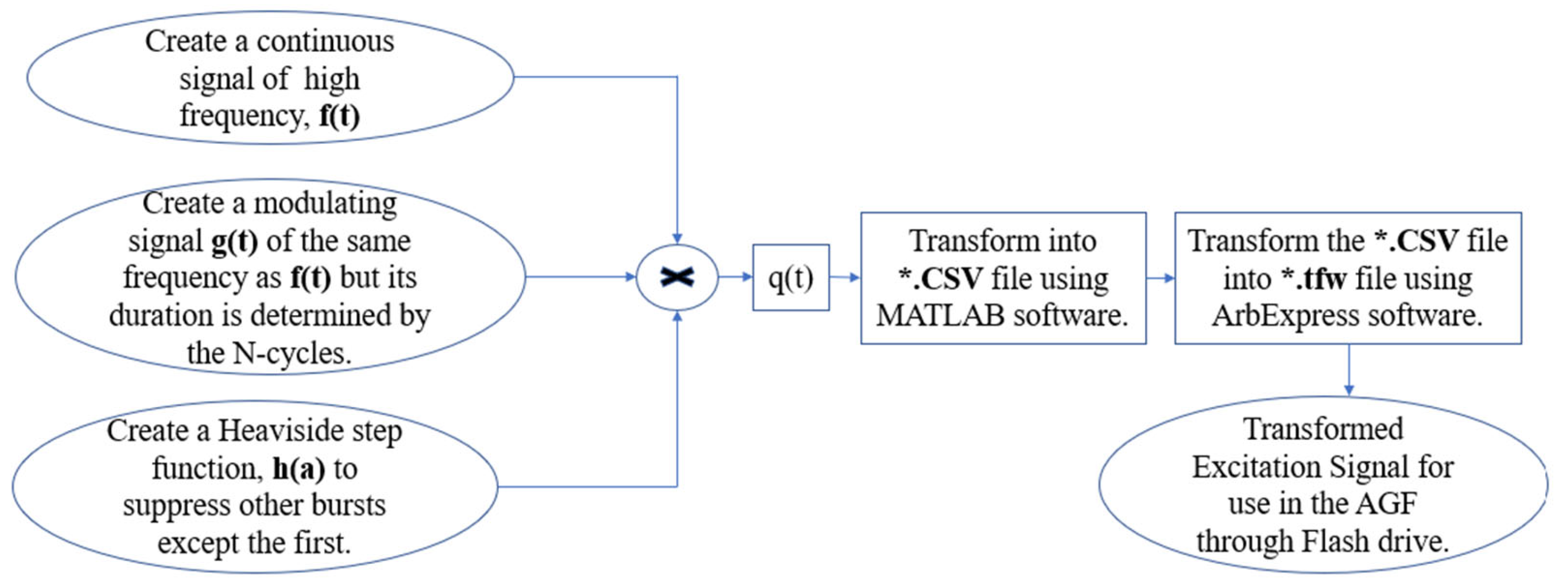
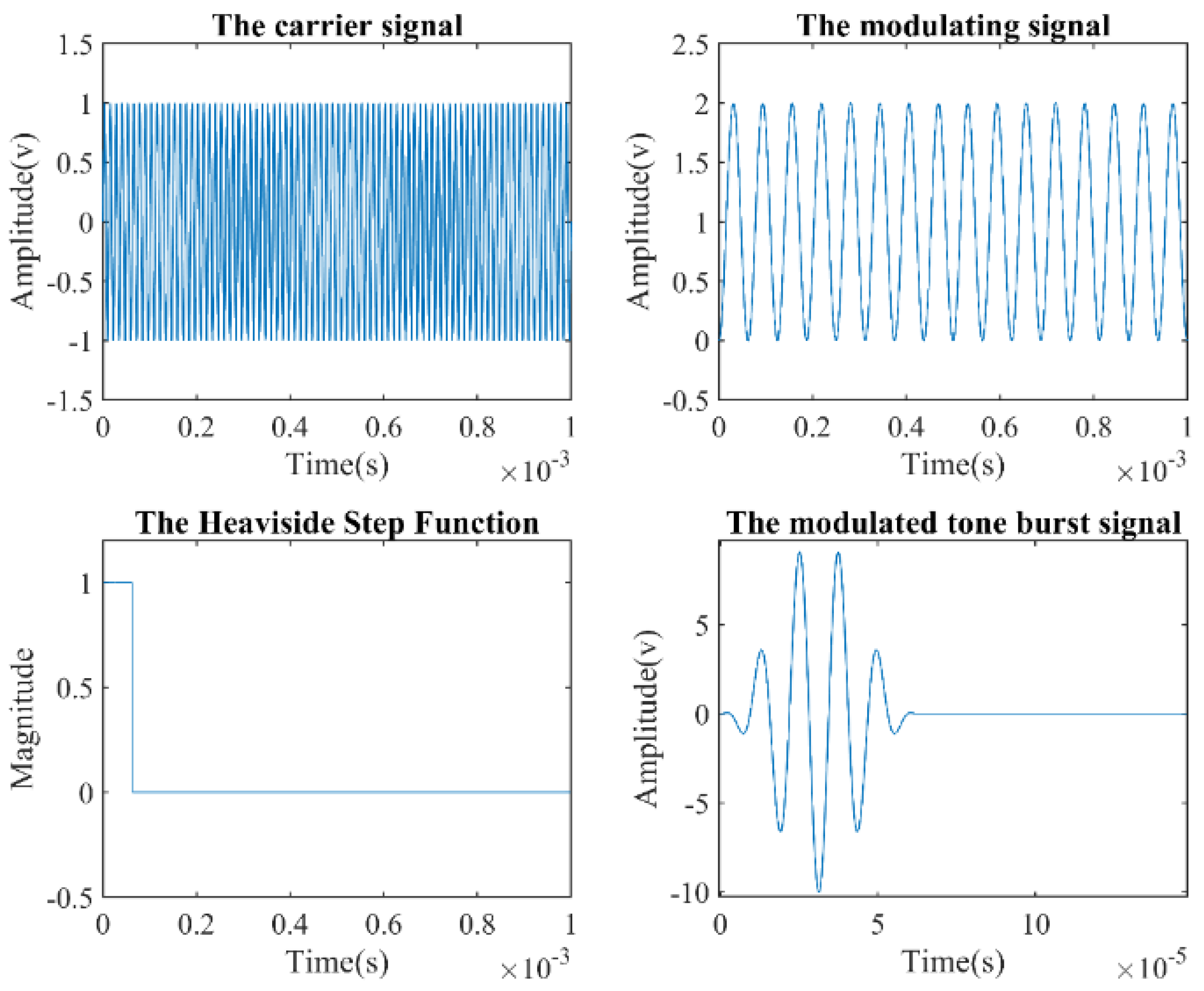
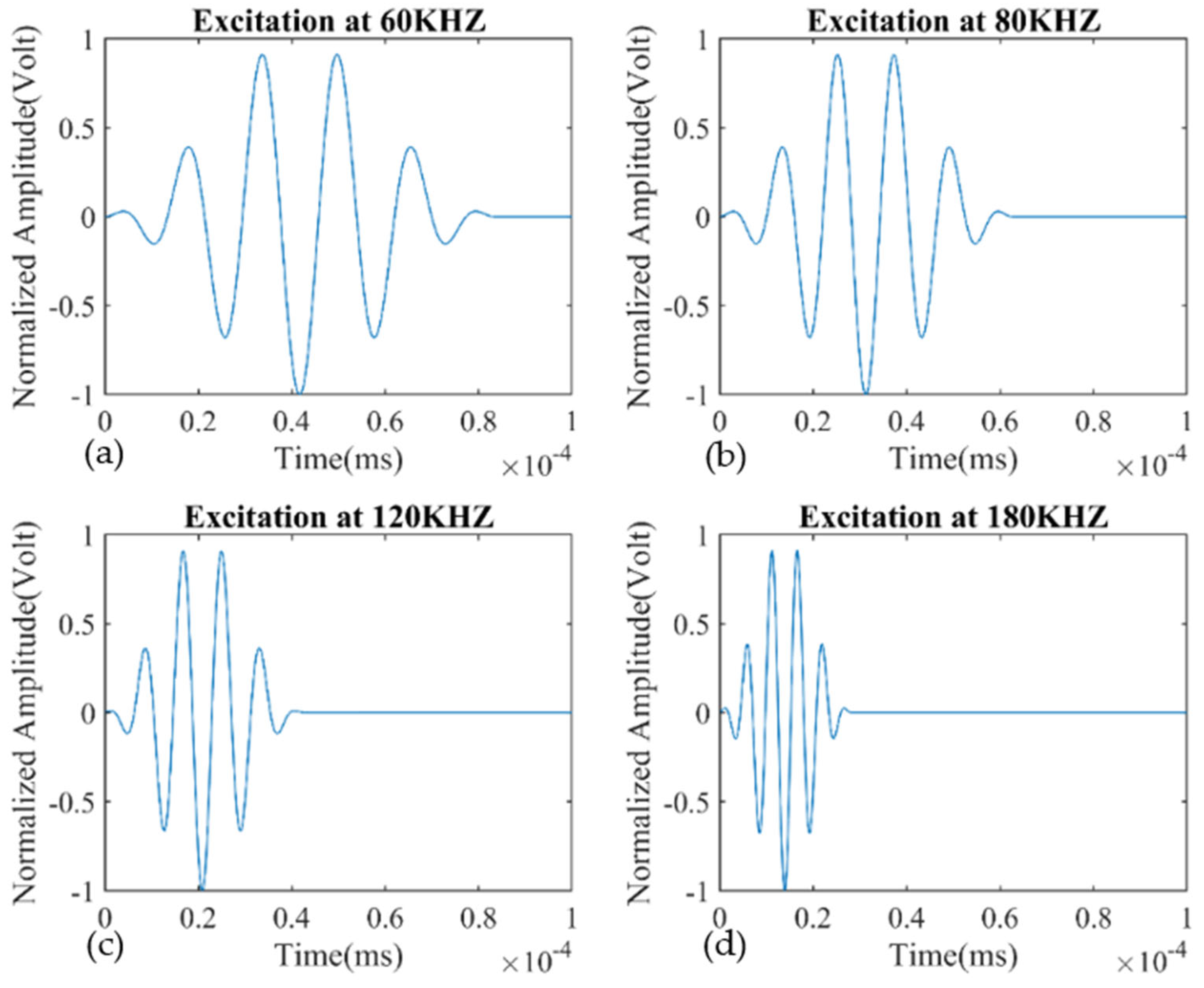
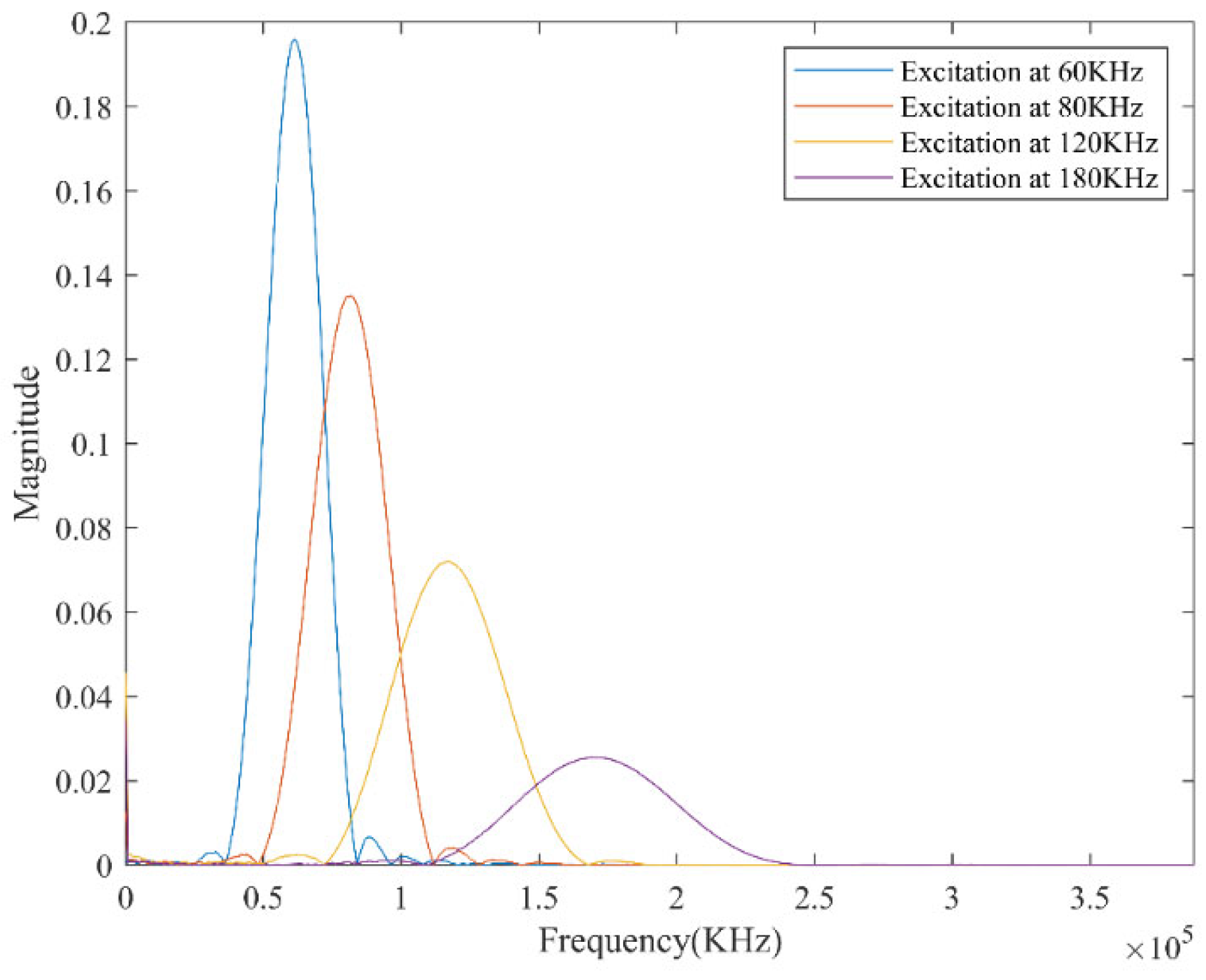
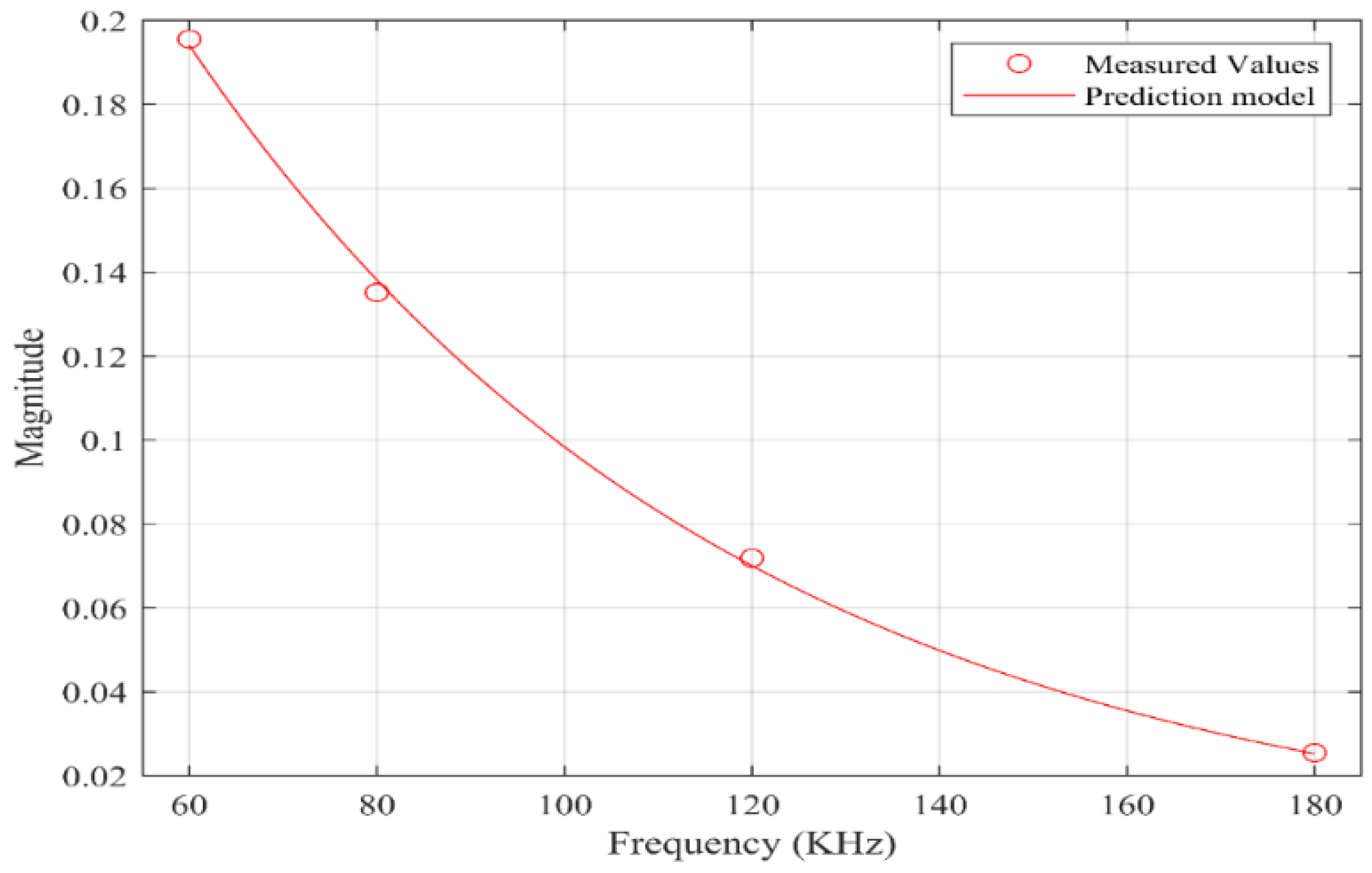
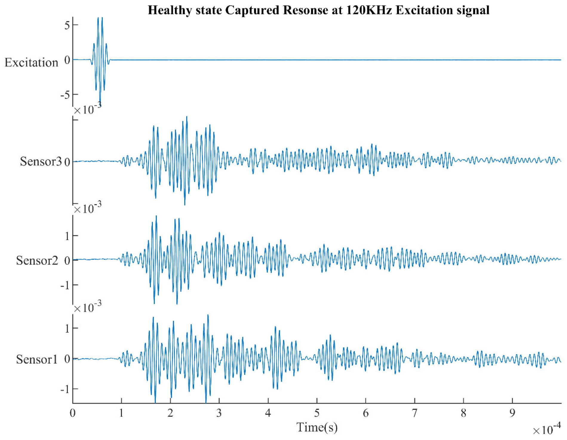
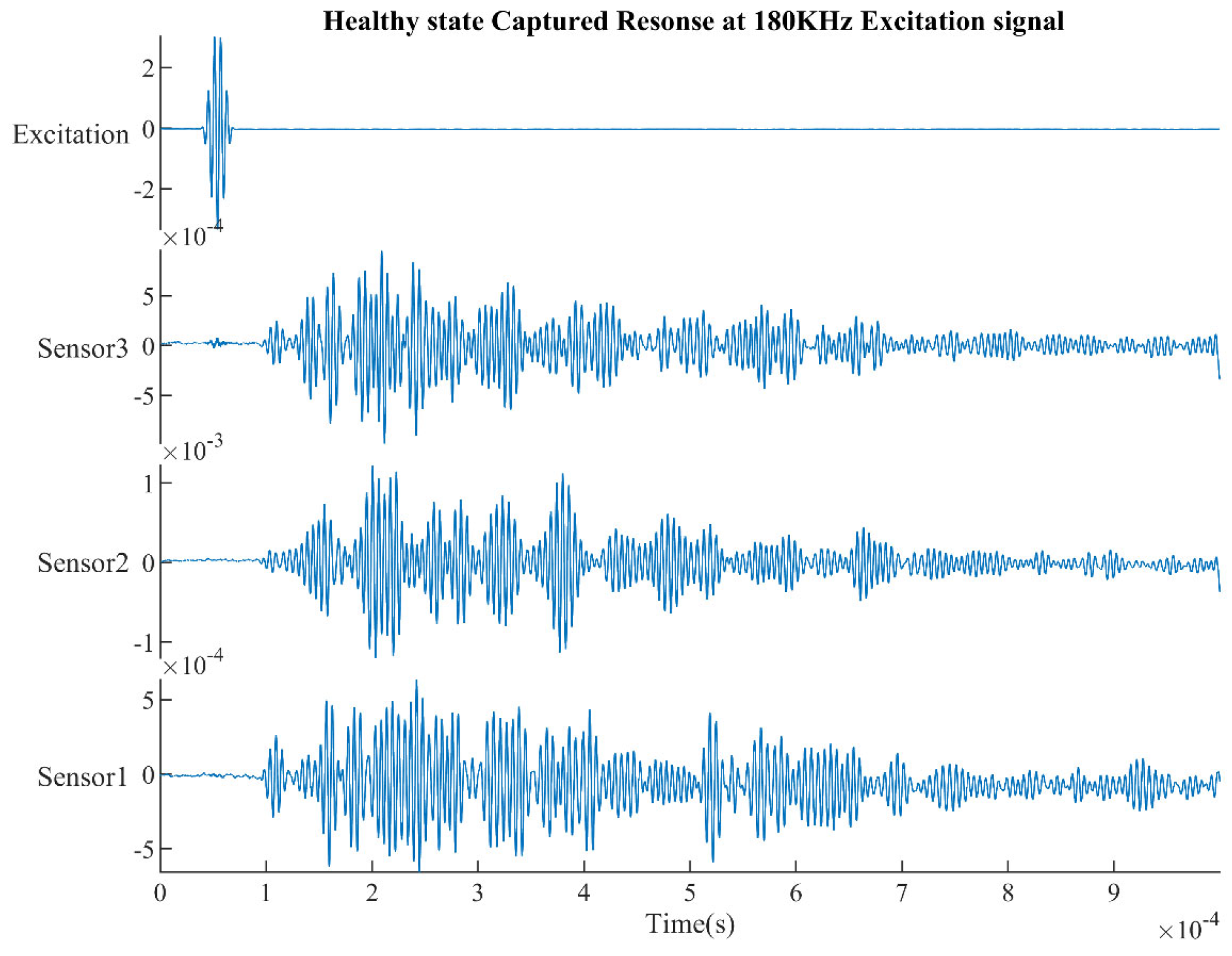
2.5. Excitation Signal Generation

As shown in the experimental setup, the circular PZT transducers are configured in pitch–catch mode, in which one of the PZTs acts as the exciter and the remaining PZTs act as the sensors. Since creating a desired tone burst signal of modulated amplitudes in the arbitrary function generator is difficult, the signal was created first in MATLAB using Equation (16) and later transferred into the arbitrary function generator.
q t = f t × g t × h ( a )
From Equation (16), three signals are needed to create a tone burst signal. One of the signals is a continuous signal of high frequency, f ( t ) , created using the probing frequency and expressed in Equation (17):
f ( t ) = A   s i n ( 2 π f t )
The second signal is the modulating signal created using the same probing frequency but with a duration bound by the N number of cycles, as expressed in Equation (18):
g t = ( 1 c o s ( 2 π f t / N ) )
The products of Equations (17) and (18) generate a signal of multiple bursts. Due to the formation of multiple bursts, a third signal function h ( a ) was introduced to extract just a burst. The signal function is as defined in Equation (19). The third signal is a step function with two possible outputs: a zero or a positive one. In this study, h ( a ) multiplied the two products of the first two signals, resulting in two possible outputs. Through the procedure shown in Figure 3, the tone burst excitation signal depicted in Figure 4 was achieved.
h ( a ) = 1             i f   a t 0             i f   a > t
Different excitation signals were created by varying their central frequencies, as shown in Figure 5. The amplitudes of the signals were normalized, and about 1.00 ms of duration was allowed before a repeat of another burst. At a relative constant velocity of the wave, the wavelength and frequency of a signal are proportionally related, as in Equation (20).
λ   1 f
Also, from the plotted excitation signals, the signal packet duration decreases as the central excitation frequency increases. This implies a decrease in the signal’s wavelength as the frequency increases. The decrease in wavelength increases the sensitivity of the signal to detect small defects. The wavelength of the excitation signal is vital for damage detection, and the probability of detecting small-sized damage increases as inspection frequency increases. Damage stands a reasonable chance of being detected when its size is larger than one-half the wavelength of the probing wave [27]. About 5 cycles were used to create the excitation signal, allowing for high signal resolution in the time domain. As shown in the frequency domain of Figure 6, the tone burst signal possessed a wide range of low and high frequencies with low harmonic content. This allowed for the detection of damage with minimal noise interference.
Hence, a tone burst of a few cycles offers a mix of a wide frequency range, short duration and minimal interference. Figure 6 depicts the frequency spectrum of the excitation signals. The result implies that low-frequency excitation signals possess more power for propagation and penetration through structures than high-frequency excitation signals [28]. This suggests a compromise on propagation distance and sensitivity to small damage as guides to selecting a suitable excitation frequency. Hence, from Figure 6, the strength of the excitation signal was modelled and expressed in Equation (16). As earlier emphasized, the actuation strength of the excitation signal decreases exponentially with increasing frequency. This suggests that high power is required to propagate high-frequency Lamb waves. The consequences would be limitations to the propagation distance and penetration extent that could have been achieved because the signal would attenuate faster than the low-frequency signal. Hence, this would necessitate preamplification of the excitation signal before use on the exciter in some studies, but this was not applicable in this study because we could capture a useful strength of the response signal at the sensing positions.
From the fitted plot of Figure 7, the magnitude of the excitation signal decreased exponentially as the frequency increased. This behavior is empirically expressed in Equation (21):
g ( f ) = a × e x p ( b f )
where a and b are constants with the values 0.5377 and −0.01698, respectively, and f is the frequency of the actuating signal.

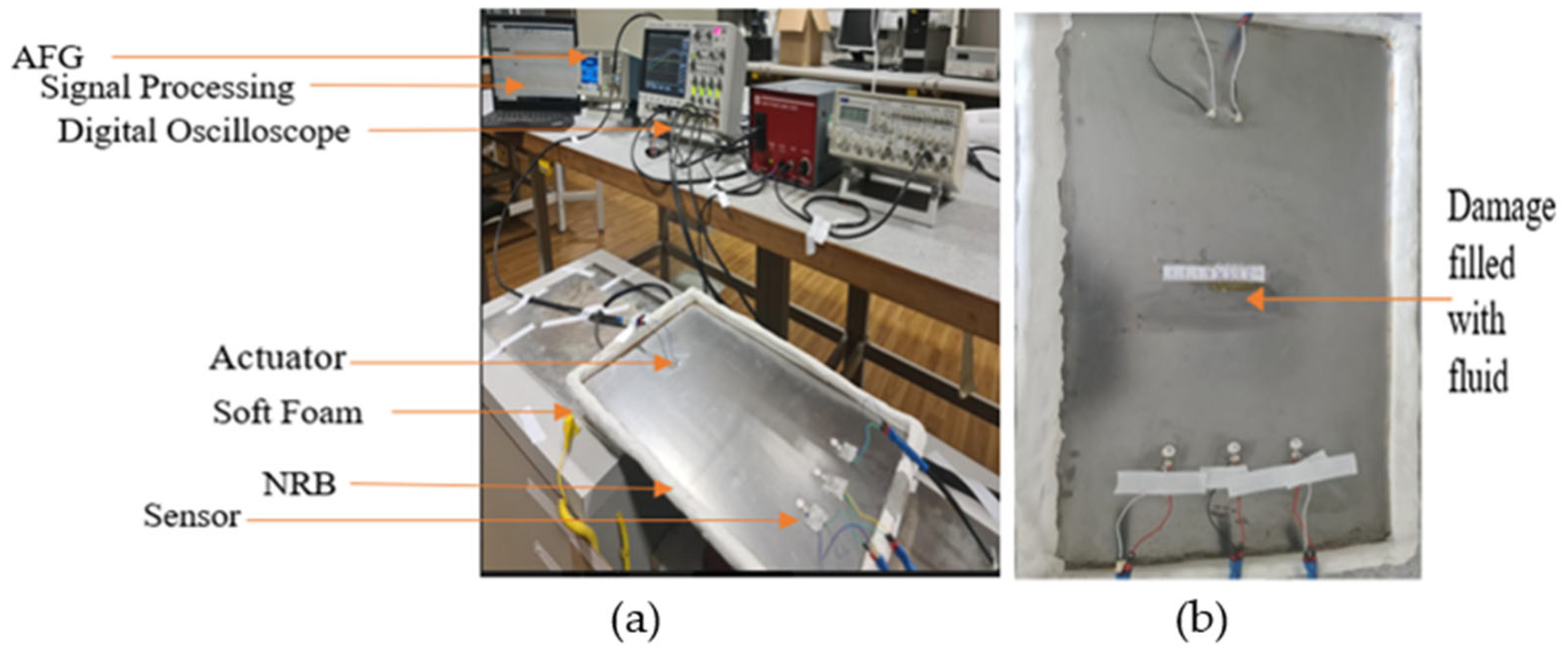
3. Materials and Methods

Two mild carbon steel plates of the same dimensions 500   m m × 300   m m × 3.00   m m were used in the study. One plate was considered a reference structure and used as the pristine plate for baseline signal acquisition, while the second plate was used to create the different damage case scenarios, as shown in Figure 8. The properties of the plate are listed in Table 1. Damage of 40.00   m m × 5.00   m m × 2.50   m m was seeded at the mid-distance between the exciter and the middle sensor. The distance between the exciter and middle sensor was 300.00   m m and allowed for proper separation of the wave modes. Prior to the installation of the transducers, acetone was used to clean the surface of the plates, which took about 5–10 min to dry [29]. The cleaning ensured the removal of unnecessary particles and oils that could hinder a proper transfer of signals between the transducers and the plate. All the ceramic transducers ( P Z T : 7.00   m m × 0.195   m m ) were of a circular type with the omnidirectional capability of radiating and receiving signals [30], unlike the rectangular counterpart that is orientation-dependent [31]. The properties of the transducers are in Table 2. The transducers were bonded on the plate’s top plane using two epoxy adhesive components [32]. The adhesive eliminated air gaps between the plate and the transducers that would ordinarily cause high impedance and limit energy transfer significantly [33].
Additionally, the applied adhesive thickness was ensured to be less than the thickness of the transducers since its thickness contributed to energy signal transfer limitations [33,34]. An arbitrary function generator, AGF (Tektronix AFG1062 function generator), was used to generate the tone burst signal excitation signals. The function generator produced excitation signals with a varying central frequency of 10 V peak–peak voltage. An Agilent Technologies oscilloscope (MSO-x 3024A, 200 MHz, 4 GSa/s) simultaneously captured the excitation and response signals. Using the 32-averaging acquisition mode, we minimized the random noise effects on the signals. Edge reflection waves are notable for causing complexity in a response signal [35]. Therefore, minimizing it was necessary, and DAS modelling air dry clays were installed around the edges of the plate to account for this effect [36]. We performed the experiments at laboratory temperature, which was relatively stable. All the captured response signals were recorded using the oscilloscope and transferred to the PC for preprocessing and postprocessing using MATLAB version 2022a. Two distinct scenarios, outlined below, were investigated using different sets of central frequencies: Set1 ranging from 60 kHz to 180 Hz, and Set2 spanning from 40 kHz to 110 kHz. The response signals from Set1 were used to estimate the influence of varying damage states on the response while those from Set2 were used for deducing the influence on the TCs of the response signals.
Case A: The base scenario.
In this instance, we acquired the baseline signals. We used the healthy plate and injected four excitation frequency signals to interact with it. The sensors recorded the responses, and the oscilloscope registered them. We conducted this at a controlled laboratory temperature of below 26 °C
Case B: The current scenario.
In this case, damage of the dimension 40.00   m m × 5.00   m m × 2.50   m m was seeded on the second plate to become an unhealthy plate. Afterwards, the damage was filled in with debris and different fluids, as given below. The response signals were captured and analyzed:
  • Empty damage
  • Debris-filled damage
  • Water-filled damage
  • Oil-filled damage
  • Grease-filled damage

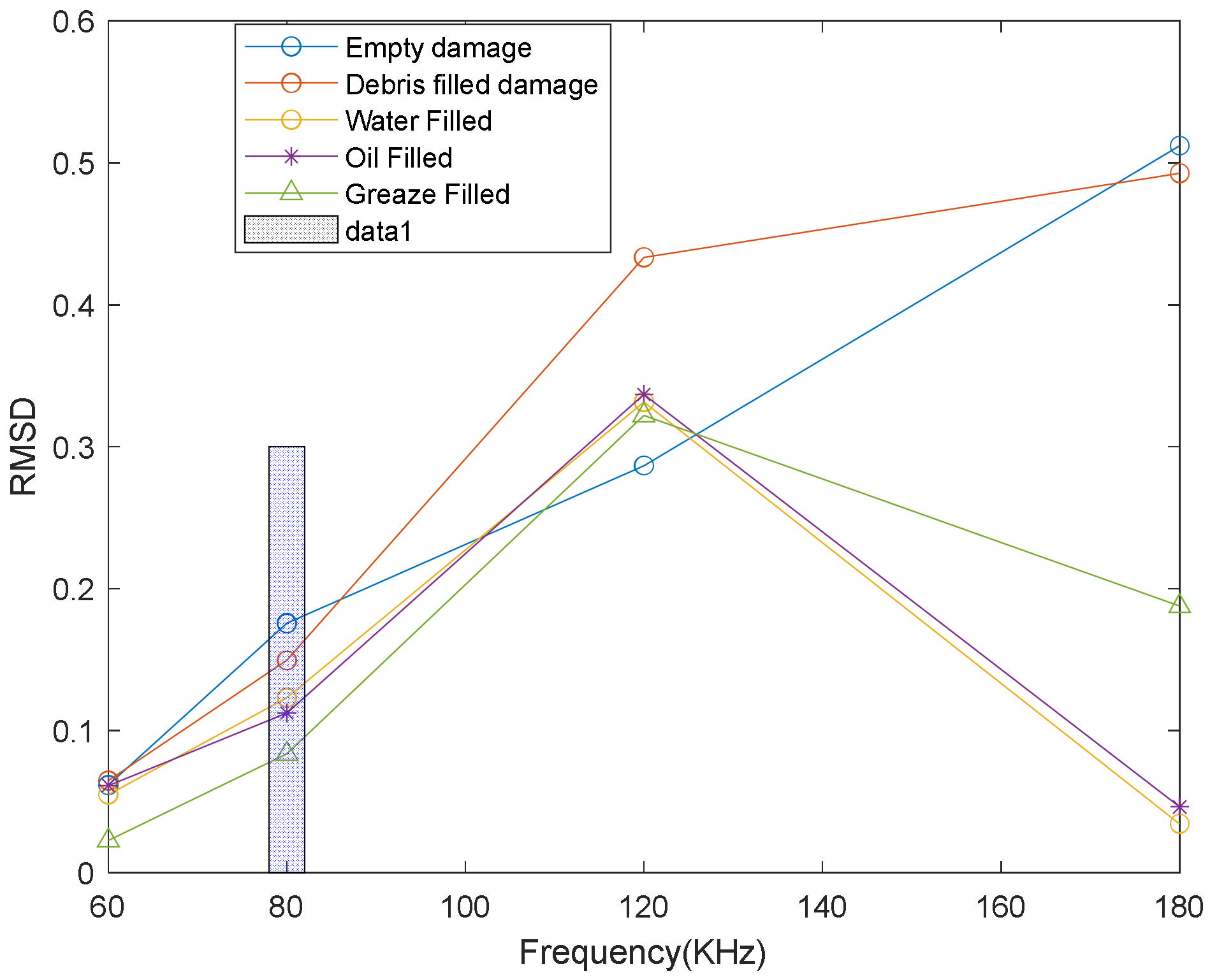
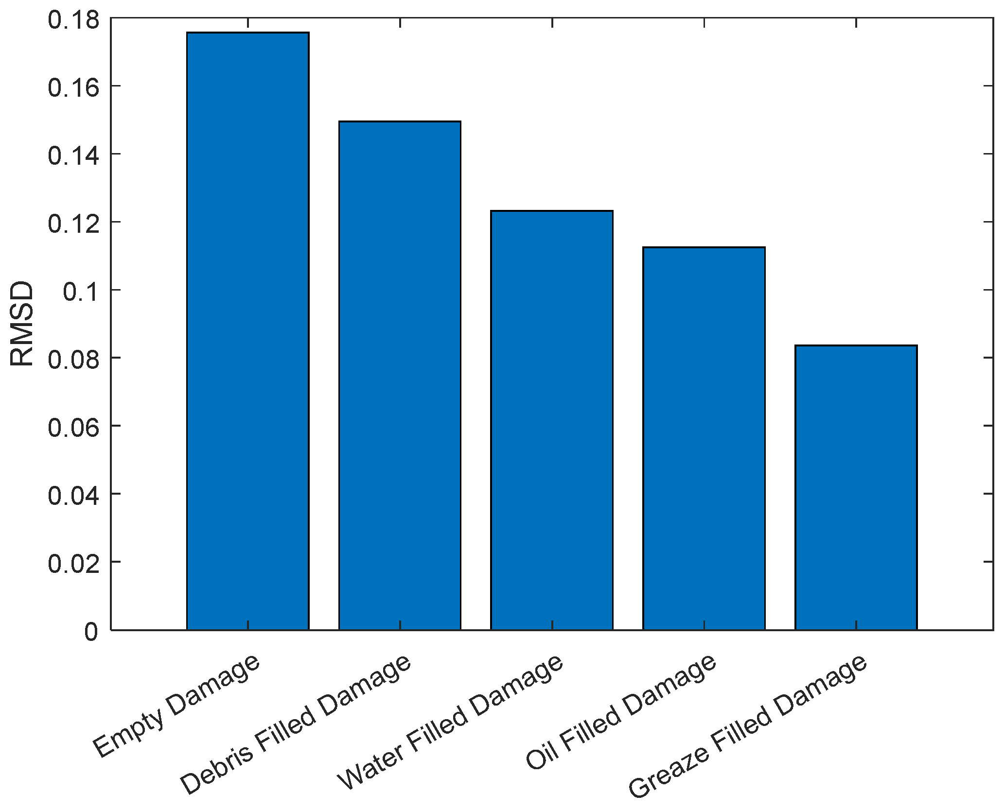
4. Results and Discussion Using the Set1 Range of Frequency

The plate responses to each excitation frequency were captured using 32 mean averaging and further smoothed. The preprocessing was applied to minimize random error effects and increase the response signal-to-noise ratio (SNR) of the response signal, thereby enhancing the signal quality. Also, most of the captured signals were either shifted above or below the time axis. The origin point was verified and accurately repositioned using the correction function outlined in Algorithm 1 to adjust for the shift in the recorded response signals. This was meant to enhance the reliable comparison of any two states of the plate scenarios.
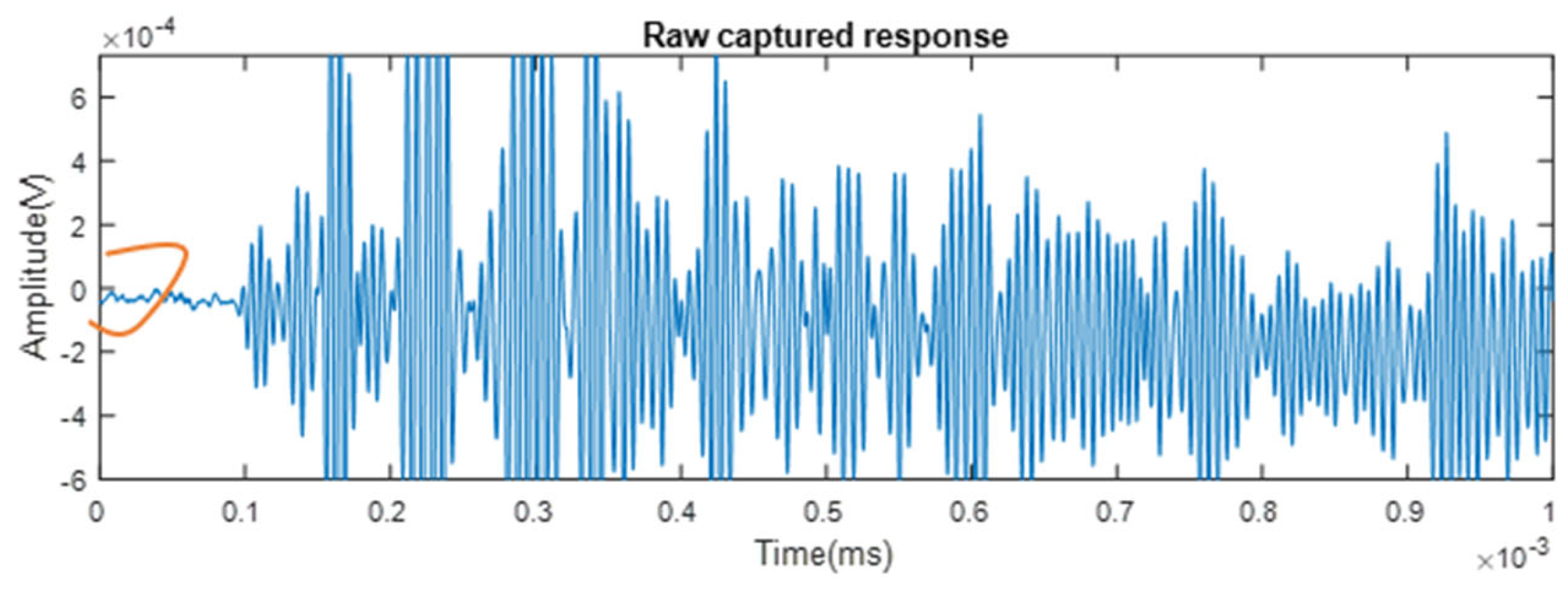
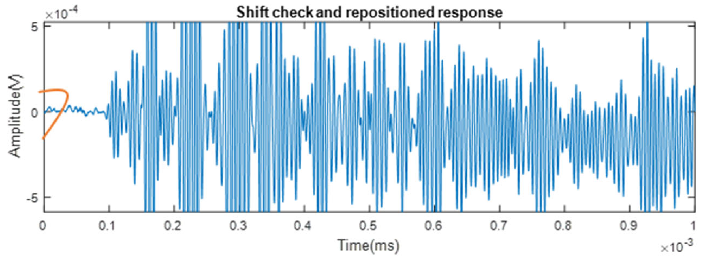
Algorithm 1 Check and Shift
1: function G = CheckandShift(x)
2:  if x(i) < 0 % Condition 1: check if the first sample point is shifted below origin 0.
3:        G = x + abs(x(i)); % If True, reposition the signal to the origin point.
4: elsif x(i) > 0% Condition 2: check if the first sample point is shifted above the origin 0.
5:     G = x − abs(x(i)); % If True, reposition the signal to the origin point.
6: elsif x(i) == 0; % the default
7:   G = x8: end
Figure 9 is a response signal captured by the sensor, S 1 , but it is shifted at the marked origin.
Hence, the correction function was applied to the response signals and repositioned as shown at the marked origin of Figure 10.
Figure 11, Figure 12, Figure 13 and Figure 14 are the time–domain plots of the response signals captured by the three sensors at various excitation frequencies of Set1. From the figures, the fundamental modes S 0 and A 0 were observed in the first two main packets of the response signals. The resolution of the captured response signals decreased as the frequency of excitation increased, making it challenging to separate the two fundamental modes with ease. The response signal captured by each sensor differed but contained the fundamental modes, which were the dominant modes. It was also noted that the electromagnetic interference (EMI) effect began to manifest with increased excitation, becoming notably evident at 120 kHz and 180 kHz. The EMI effect manifested as the initial wave packet in the response signal, albeit with diminished amplitude. This EMI may result from instrument noise or RFI devices within the laboratory. However, it does not change the signal modes of interest in the captured response signals and needs not be misinterpreted as a structural response signal. It can be removed using a filter but this was not applicable here because it did not compromise the required modes of the response signals.
In the time domain of the response signals, the fundamental modes prevail. Figure 15 illustrates this, showcasing the healthy plate response signal captured by S2 upon injecting an 80 kHz excitation signal into the plate. The fundamental symmetric mode S 0 was registered before the fundamental antisymmetric mode A 0 , suggesting it to be the fastest mode, although the antisymmetric mode was the dominant mode. The maximum peak of the modes was extracted from the response signals for every applied excitation signal of specific frequency using Equation (10). An effective response signal amplitude was determined by averaging the amplitude of the fundamental modes captured by all the sensors at a given excitation frequency using Equation (9).
Figure 16 shows that the average intensity of the response signal decreased as the frequency increased. The increase in attenuation as frequency increased could be attributed to more interactions between the wave signals and the structure since the wavelength was becoming sizeable to the molecular constituent of the plate, resulting in energy loss due to more scattering. Also, higher-frequency ultrasonic waves tend to be more strongly absorbed by the material through which they propagate. The absorption of ultrasonic energy by a medium is frequency-dependent, and certain materials exhibit increased absorption at higher frequencies. This absorption decreases the intensity of the ultrasonic-guided waves as they propagate through the material. However, the intensity of the antisymmetric fundamental mode is greater than that of the fundamental symmetric modes by an average of about 10%, making it a dominant mode. On the consideration of dominance, the fundamental antisymmetric mode A 0 was selected and used to assess the health state of the plate. Also, in both the fundamental symmetric and fundamental antisymmetric modes, it was observed that the signal amplitude started decreasing after 80 kHz. This suggests that 80 kHz was the optimum frequency for this study as it possessed the highest response energy, although crack detection was better with a higher frequency but at the expense of additional power requirements.
(a)
Comparing empty damage and the pristine condition
The pristine condition of the plate was compared with the open damage condition of the plate. An RMSD of the conditions was computed using Equation (8) for every given frequency. Figure 17 shows the RMSD deviation between the pristine condition and empty damage using the average amplitude of the fundamental antisymmetric mode. It has been observed that deviation increases linearly with frequency. The increase in the RMSD value suggests better damage detection at higher frequencies because damage detection is wavelength-dependent. It is worthy of note that damage has a higher chance of detection if its size is larger than the probing wavelength [14]. From the linear fitting of the observation data, an empirical regression model with an R 2 of about 0.97 was deduced and expressed in Equation (22). The model is good since it could account for about 97% of the variation in the structural response at a given excitation frequency.
y E D ω = 0.0036 ω 0.1386
(b)
Damage filled with dry debris and a plate of pristine condition
Figure 18 shows the variation between the pristine condition and damage filled with the debris condition of the plate. It was observed that there was a linear relationship between the health state variation in the plate and the frequency of inspection. The variation between the two conditions increased as frequency increased due to a decrease in the signal’s wavelength, which would enhance more wave–damage interactions. Particularly, the wave-scattering effect would increase as corrosion debris filled the damage and introduced rough surfaces and edges to the damage. The increase in wave–damage interaction resulted in wave-scattering energy loss and manifested as a reduction in the signal amplitude. An empirical model for the filled-in damage response is as in Equation (23), with an R2 value of about 0.73 and RMSE of about 0.15. The predictive model is good and could account for about 73% variation in the response signals due to frequency changes.
y D F D ω = 0.0038 ω 0.1101
(c)
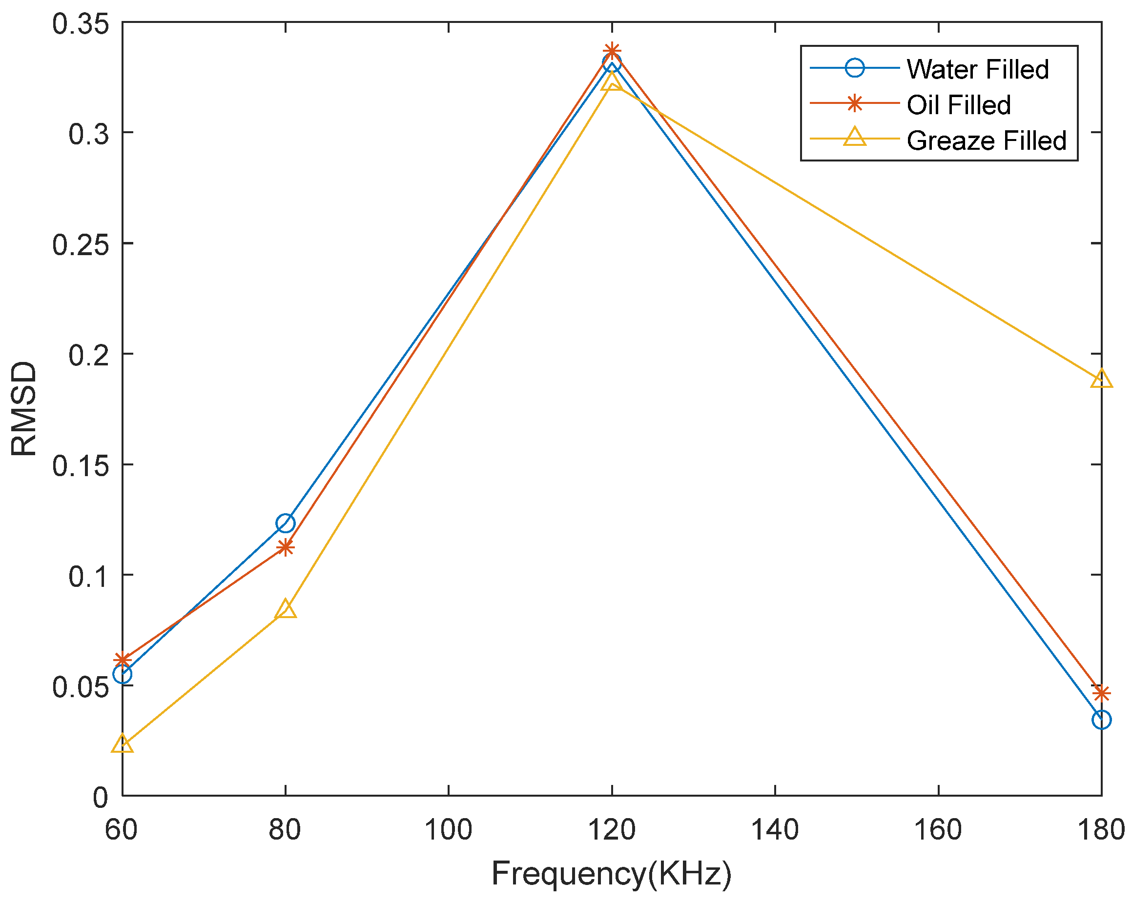
Damage filled with different fluids and the pristine condition of the plate
Figure 19 shows the deviation between the pristine condition of the plate and damage filled with different fluids in the plate. The three fluids (water, oil and grease) that filled the damage have different viscosities. The viscosity is the resistance of fluid to deformation. Hence, water is less viscous than oil and grease, while oil is less viscous than grease. The Lamb waves propagated through the damage and interacted with the fluid. During the interaction, partial reflection, attenuation and transmission of the wave at the boundaries of the damage occurred. It was observed that there was variation in the response signal when compared across the filled fluid. The interaction resulted in signal amplitude variations as the frequency of the inspecting wave increased. Also, it was observed that deviation changes with viscosity, which was more distinct at 80 kHz. The relationship between the frequency and the damage index was linear until after 120 kHz. The predictive model based on the region of linearity is expressed in Equation (24) through Equation (26) and plotted in Figure 20.
For damage filled with water:
y W F D ω = 0.004693 ω 0.2367
For damage filled with oil:
y O F D ω = 0.004737 ω 0.2402
For damage filled with grease:
y G F D ω = 0.005129 ω 0.3017
(d)
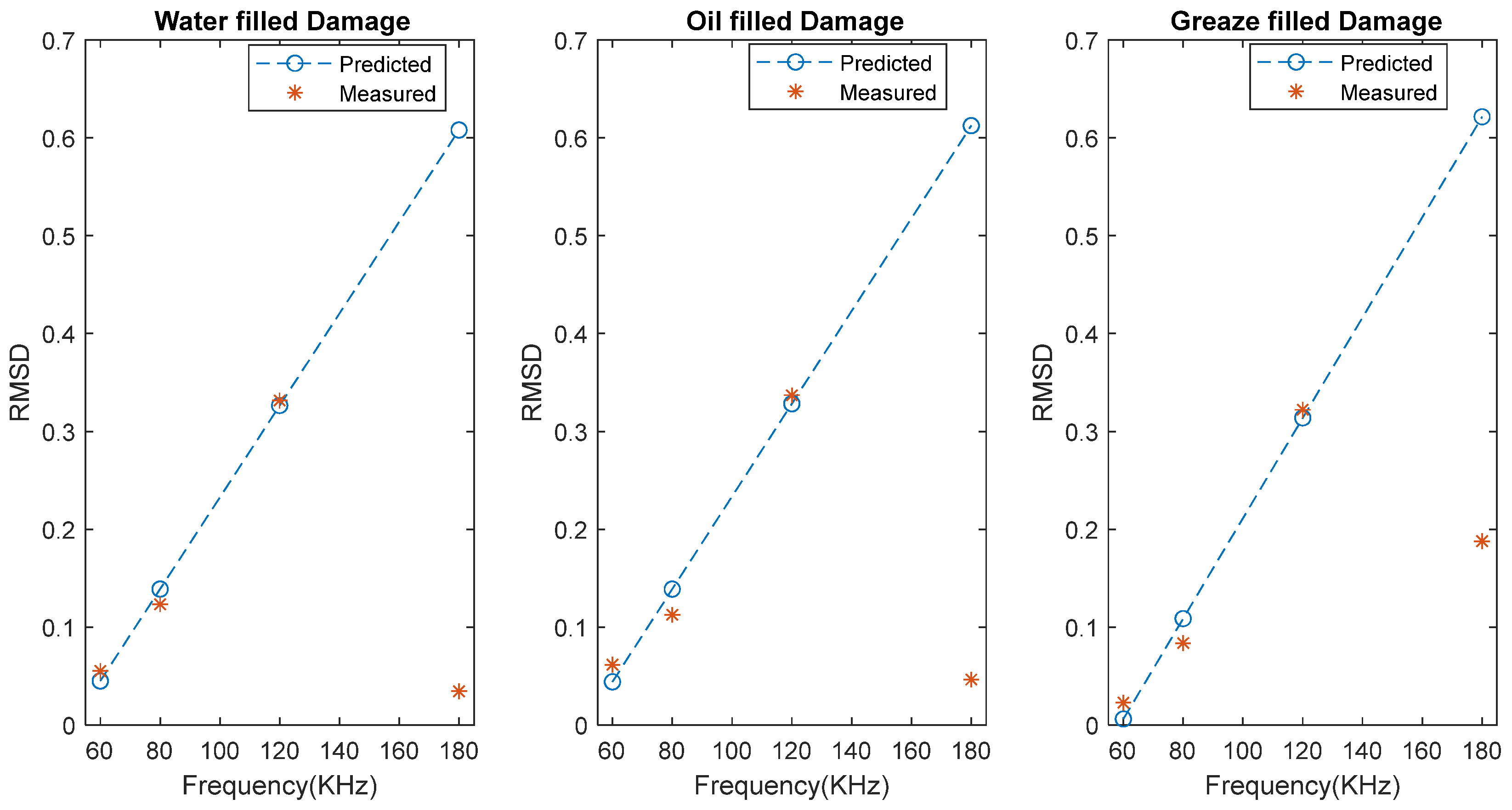
Comparing empty damage, damage filled with different fluids, damage filled with dry debris and a plate of pristine condition
Figure 21 shows the deviation of damage filled with different fluids from the pristine condition of a plate as the excitation frequency increased.
At an excitation frequency of 80 kHz, the responses were separated from various filled damage scenarios, unlike any other frequency, as shown in Figure 21. The high deviation with empty damage was due to the combinatory effect of wave scattering from the tip edges of the damage and attenuation of the transmitted wave signals. From Figure 22, the deviation of damage filled with debris from an empty damage was much greater than deviations obtained when different fluids filled in the damage. Also, the deviation of the damage filled with different fluids decreased as the fluids varied based on their viscosity. This suggests that fluid inhibits the edges of the damage from scattering the incident wave and that increases as the fluid becomes more viscous and allows much wave propagation, unlike damage filled with dry debris with unsmooth damaged edges which would enhance wave scattering.

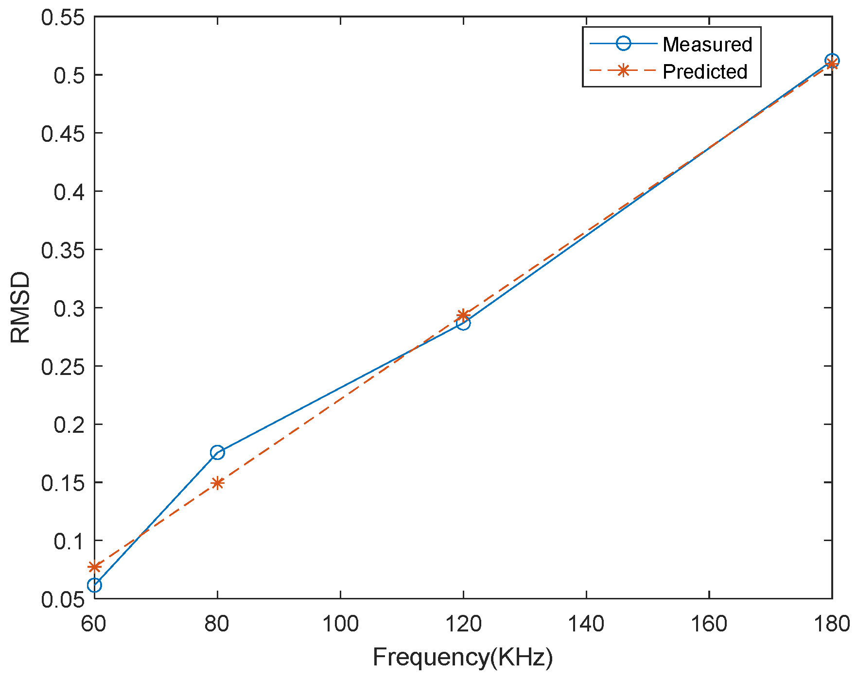
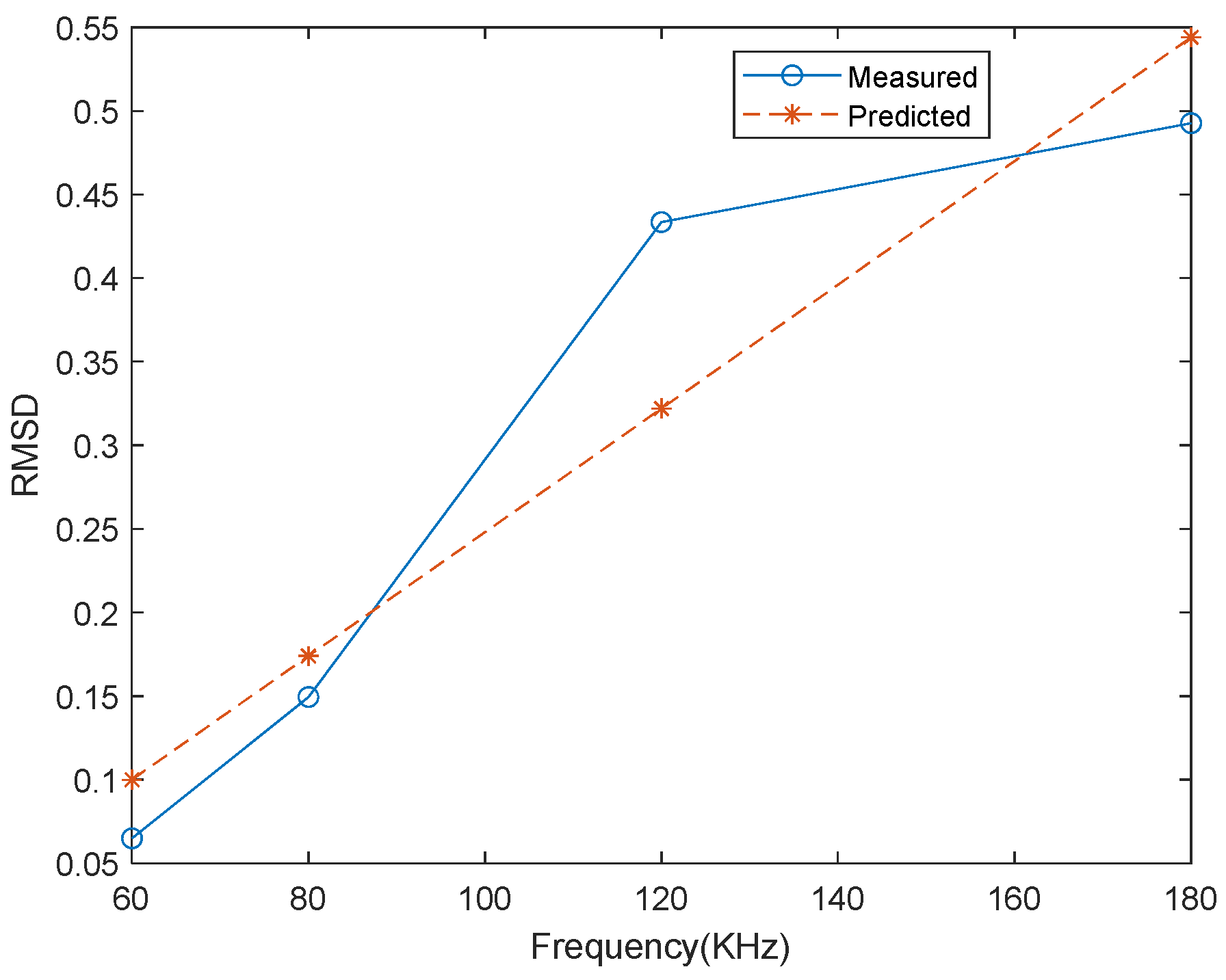
5. Results and Discussion Using a Set2 Range of Frequency

In Set2 of the frequency range, the exciter’s position was adjusted, resulting in a distance of 210.00 mm between it and the sensor for both healthy and unhealthy cases. In the damage case, the exciter was 60.00 mm from the damage, and the sensor was 150 mm from the damage. All the conditions of the Set1 range of frequencies were maintained. A frequency from 40 kHz to 110 kHz at an increasing interval of 10 kHz was used to repeat Case A and Case B of the Set1 frequency range experiments. Within the Set2 frequency range, the EMI that started from 120 kHz was highly minimized. The capability of the TC to act as an indicator of damage and to classify the type of damage was examined using only the signals collected by Sensor2, the sensor positioned in the middle.
(a)
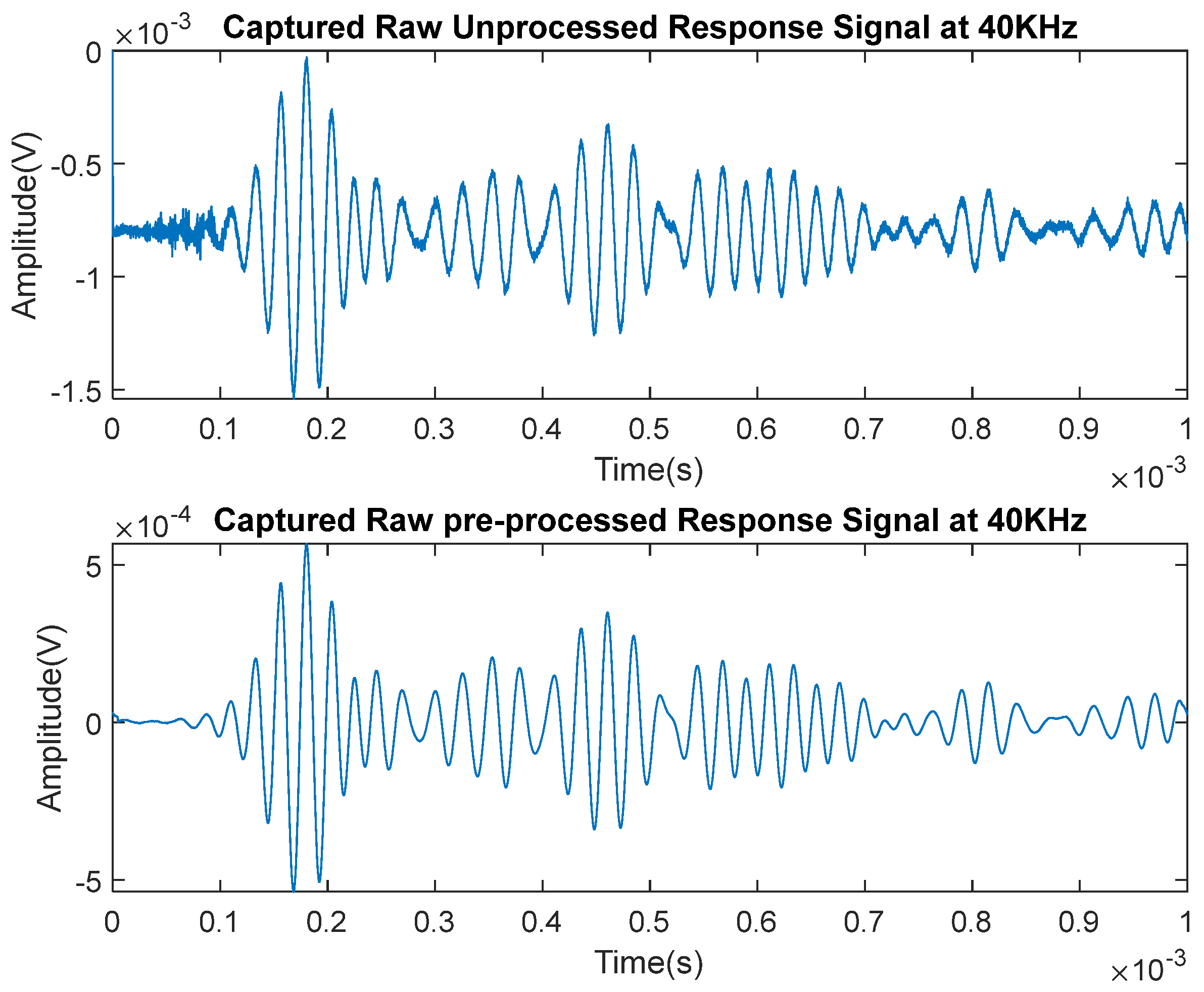
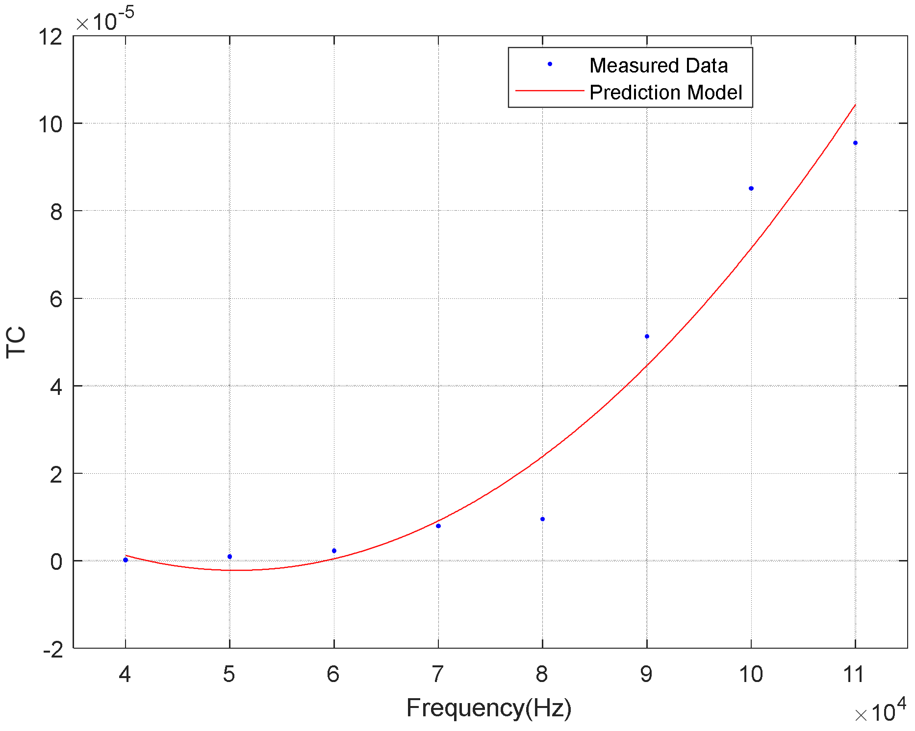
Preprocessing of the Response Signals
Figure 23 depicts captured response signals before and after preprocessing. The captured response signals were shifted from the center with noise. Hence, each captured response signal was detrended of linear and polynomial trends, which returned the response signal to the origin axis. Noise in the signals was eliminated using moving averaging techniques, and then the signals were smoothed, as illustrated in Figure 23.
(b)
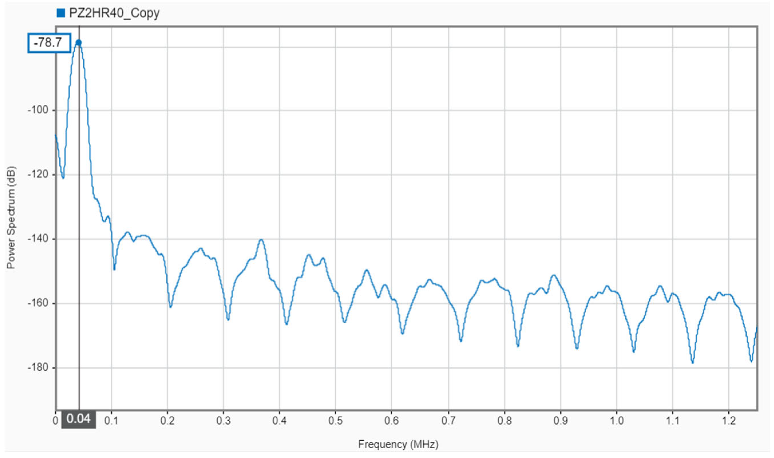
The Transmission Coefficient (TC) Deduction
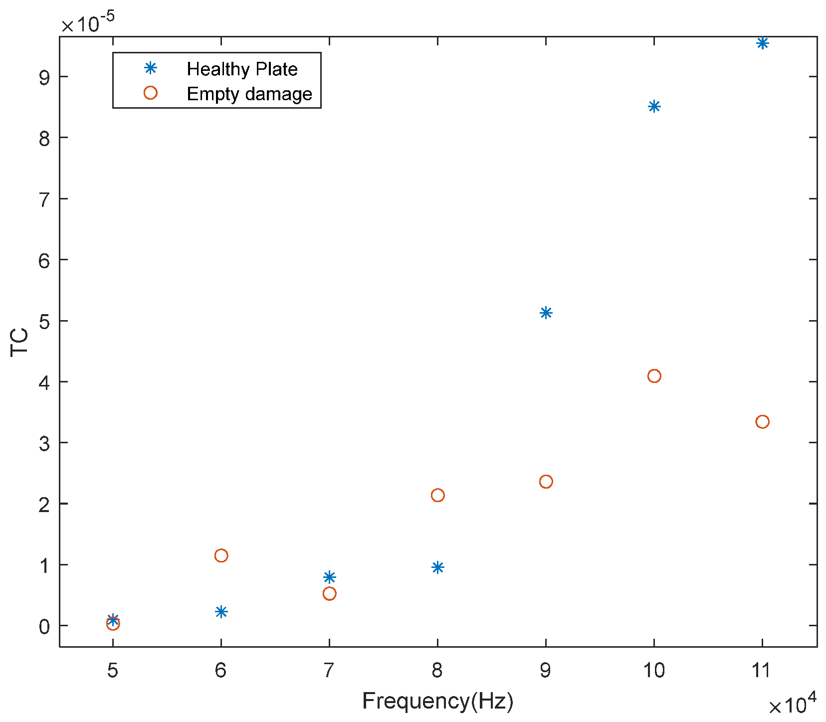
The transmission coefficient (TC) was obtained as a function of signal frequency.
Figure 24 depicts the baseline response signal via the power spectrum due to a 40 kHz excitation signal using Equation (12). The deduced signal power in dB was converted into real signal power in watts using Equation (15), while Equation (11) was used to calculate the transmission coefficient.
Figure 25 depicts the baseline TCs from the healthy plate. It was found that the TC monotonically increased with the propagating frequency of the signal. However, the rate of increase was not constant, but the increase suggests that higher frequencies were generally more sensitive to detecting changes in the structure. Hence, TC, as a function of the central frequency of the propagating wave, fitted well into a polynomial equation model (27). The R 2 of the model was about 95.26% with an RMSE of 1.029 × 10 5 when the model result was compared with the measured result. This suggests that the model is good and could account for about 95.26% variation in the response signals:
T C ( f ) V e = a f 2 + b f + c
where f is normalized by the mean 7.5 × 10 4 and standard deviation of 2.449 × 10 4 with a constant of c = 1.574 × 10 5 .
(c)
Comparing the TCs of the healthy and empty damage plates
Figure 26 is a comparative plot of healthy plate response TCs and those of empty damage. The comparative behavior of the two responses suggests that the TC varied non-monotonically across different frequencies. However, the empty damage surpassed the healthy plate significantly at 60 kHz and 80 kHz, while at other frequencies, the healthy plate tended to have a higher TC value with wider deviation. This resonates with the fact that as wave frequency increases, its scattering tendency increases, thereby creating a high probability of detecting smaller damage in the structure. The results indicate that TC values can fluctuate notably with small variations in damage features, highlighting its high sensitivity in damage detection.
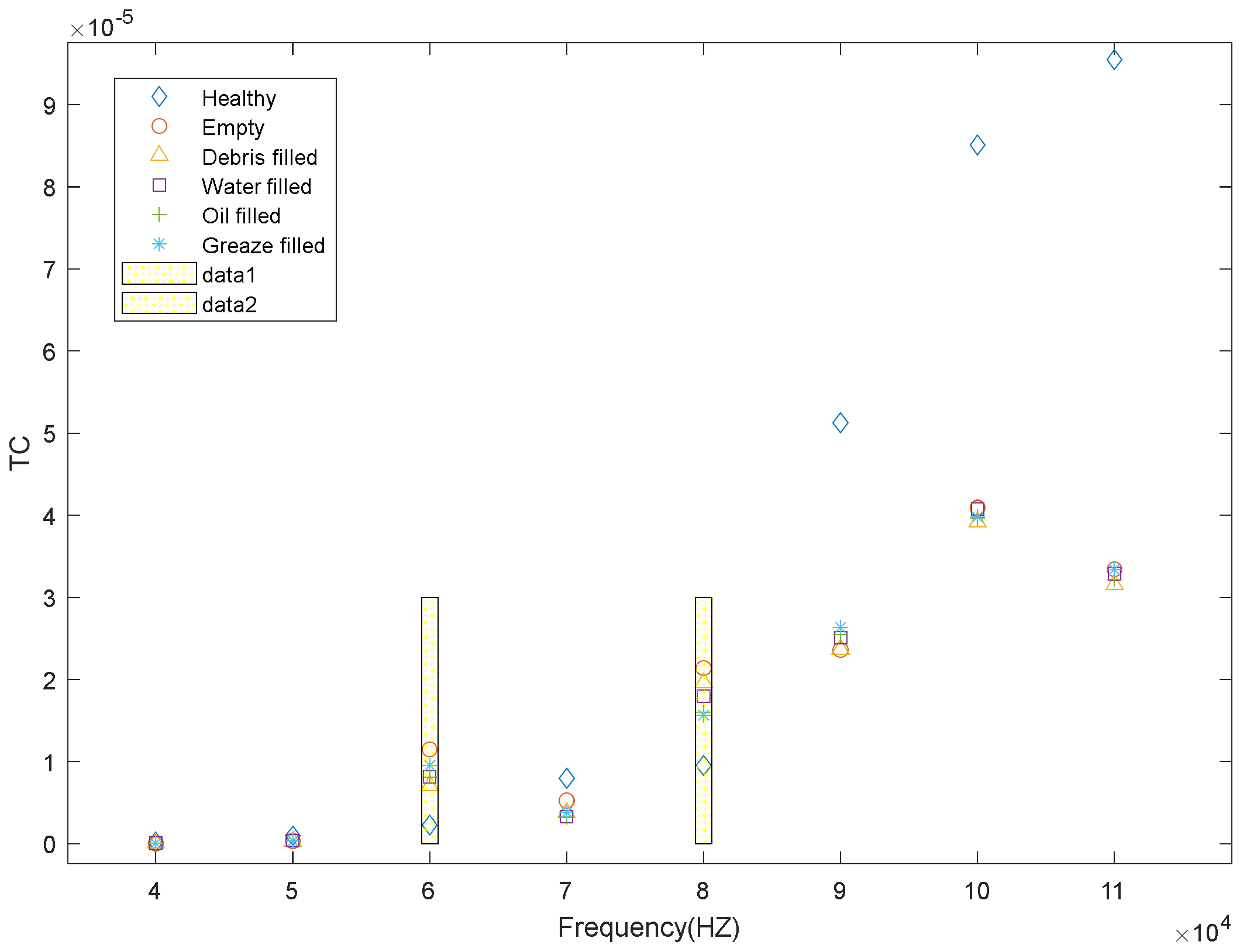
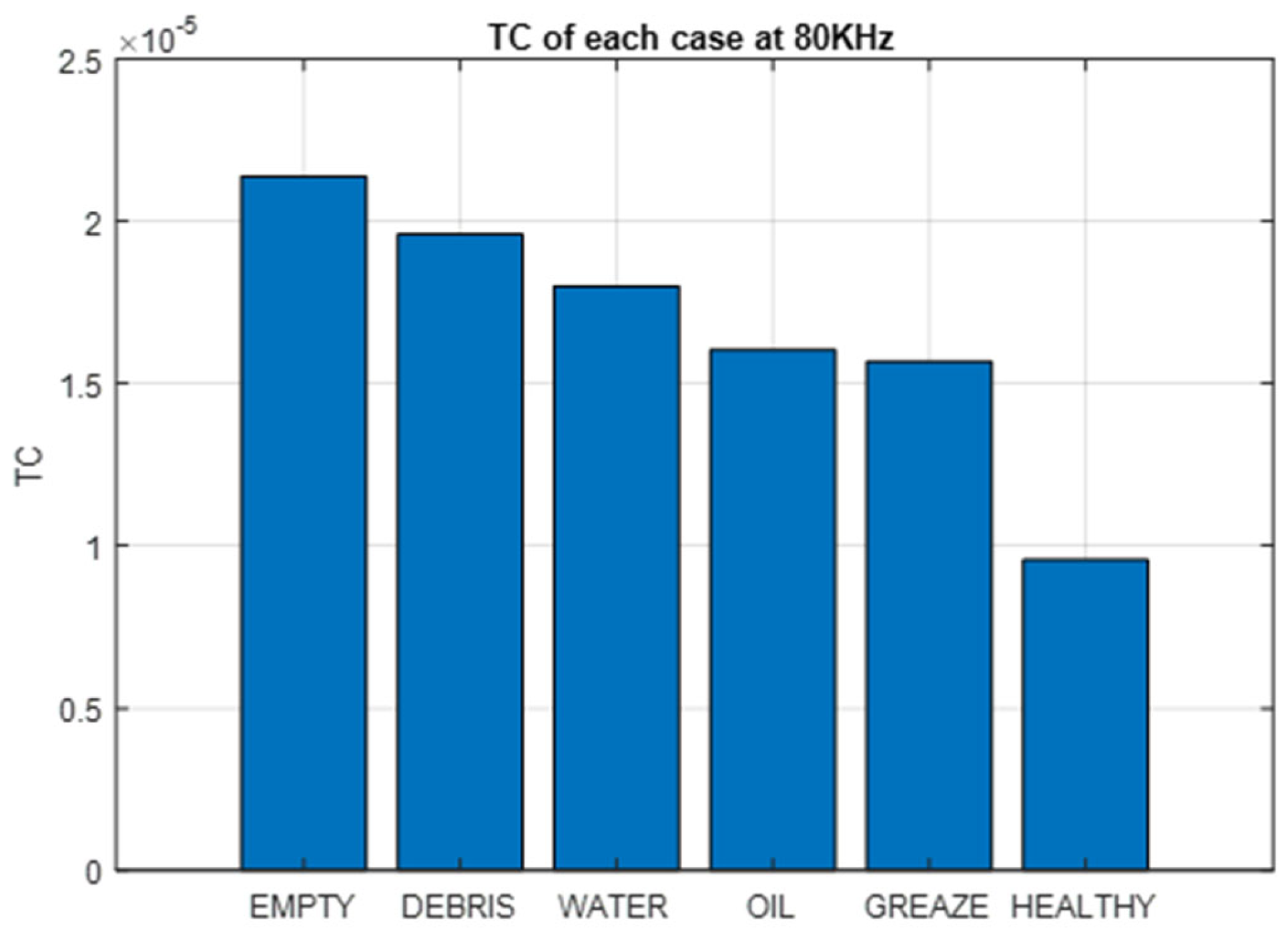
  • (d) Comparing the TCs of the healthy plate, empty damage plate and different filled cases of the damage
Damage can develop in structures and potentially be filled with different impurities, leading to its closure. It then becomes necessary to investigate the suitability of the TC in detecting and classifying the different cases. Figure 27 illustrates that across nearly all frequencies, the healthy plate exhibited the least attenuation of the propagating wave. On the other hand, the empty damage and different cases of filled damage indicated high attenuation to TC values, especially at high frequencies. This was due to increased scattering of the wave signal since the wavelength of the propagating wave decreased to the damage size as the frequency increased, resulting in more attenuation. Interestingly, at 60 kHz and 80 kHZ, the empty damage showed significantly higher TCs, making it easier to distinguish from the healthy plate and other damage cases at these frequencies. The TCs at 80 kHz were more distinctive in classifying different forms of a damage state, making it an optimal frequency for detecting and classifying damage, as TCs varied significantly across the cases. This is shown in Figure 28. This result aligns well with that of the RMSD in Figure 21, where 80 kHz of the edge-scattered signals captured by the three sensors could classify different cases of damage filled with substances. Hence, this validates an 80 kHz signal as a suitable optimal central frequency for classifying different situations of the detected damage using a TC or an RMSD as an indicating parameter.

6. Conclusions

Structures are designed to function optimally, but damage can limit their performance. It becomes vital to monitor structures for early damage detection and assessment. Unidentified damage can lead to devastating failures, resulting in the loss of lives and high economic assets. The nature of most studied or investigated damage using structural health monitoring schemes has been empty damage, while in reality, formed damage can trap substances and become closed. This damage is mainly found in the valuable assets of the oil and gas sector, where safety is a top priority. Hence, we investigated the influence of damage filled in with a substance using the pitch–catch technique of guided wave ultrasonics. A pitch–catch method of three sensors and an exciter were configured to monitor variations in the characteristic parameters of the ultrasonic-guided wave response signals due to changes in the substances that filled the damage using the statistical RMS and RMSD of the captured signals when Set1 frequency was used. Similarly, a pitch–catch of one exciter and one sensor was configured for the same study using variation in the transmission coefficients (TCs) of the captured response signals but with more frequency signals between 40 kHz and 110 kHz. As illustrated in Figure 3 and Figure 4, an amplitude-modulated five-cycle tone burst excitation signal was systematically created and used to perform the study. The selected frequencies, especially in the first experiment, were such that only fundamental modes were prominent and distinct in the response signals. The fundamental antisymmetric mode A 0 was found to be dominant and more sensitive than the fundamental symmetric mode S 0 for variation in substances that filled in the damage. It was found that variations in the damage states were directly proportional to the increased signal frequency. Although linearity exists, an increase in frequency entails a decrease in wavelength and an increase in interactions with more particles, leading to fast energy loss. In the first experiment, a sharp drop in deviation was observed immediately after 120 kHz across all the media that filled in the damage. This is attributed to significant energy loss due to the decreased wavelength, which allowed for more wave–particle interactions. In both experiments, the 80 kHz excitation signal distinctively detected and classified damage filled with different substances in the same order of empty damage to the grease-filled damage. The two experiments inevitably suggest that an 80 kHz excitation signal is optimal for detecting and classifying damage filled with different substances. Also, empirical predictive models were deduced and would be vital to improving algorithm schemes for structural health monitoring, especially in the oil and gas sector, where this type of studied damage is inevitable. Further study is suggested on geometrical variation detection and quantification using the two approaches. Additionally, the suitability of the methods, especially the TC under varying environmental conditions, is suggested for further study.

Author Contributions

S.C.O.: draft preparation, writing and editing. M.A.K.: review and supervision. A.S.: administrative approvals and supervision. All authors contributed to the paper and approved the submitted version. All authors have read and agreed to the published version of the manuscript.

Funding

This research was funded by the Petroleum Technology Development Fund (PTDF) of the Federal Government of Nigeria (Grant No.: PTDF/ED/OSS/PHD/SCO/1520/19).

Data Availability Statement

The data presented in this study are available upon request from the corresponding author. The data are not publicly available because they form part of an ongoing study.

Acknowledgments

The authors acknowledge the funding support from the Petroleum Technology Development Fund (PTDF) of the Federal Republic of Nigeria and the University of Nigeria (UNN).

Conflicts of Interest

The authors declare no conflict of interest.

References

  1. Musmar, M.A. Structural performance of steel plates. Front. Built Environ. 2022, 8, 991061. [Google Scholar] [CrossRef]
  2. Fromme, P. Corrosion Monitoring Using High-Frequency Guided Waves. Available online: http://www.ndt.net/?id=23235 (accessed on 8 April 2022).
  3. Olisa, S.C.; Starr, A.; Khan, M.A. Monitoring evolution of debris-filled damage using pre-modulated wave and guided wave ultrasonic testing (GWUT). Measurement 2022, 199, 111558. [Google Scholar] [CrossRef]
  4. Zai, B.A.; Khan, M.A.; Khan, K.A.; Mansoor, A.; Shah, A.; Shahzad, M. The role of dynamic response parameters in damage prediction. Proc. Inst. Mech. Eng. Part C J. Mech. Eng. Sci. 2019, 233, 4620–4636. [Google Scholar] [CrossRef]
  5. Zai, B.A.; Khan, M.A.; Khan, S.Z.; Asif, M.; Khan, K.A.; Saquib, A.N.; Mansoor, A.; Shahzad, M.; Mujtaba, A. Prediction of crack depth and fatigue life of an acrylonitrile butadiene styrene cantilever beam using dynamic response. J. Test. Eval. 2020, 48, 1520–1536. [Google Scholar] [CrossRef]
  6. Giurgiutiu, V.; Gresil, M.; Lin, B.; Cuc, A.; Shen, Y.; Roman, C. Predictive modeling of piezoelectric wafer active sensors interaction with high-frequency structural waves and vibration. Acta Mech. 2012, 223, 1681–1691. [Google Scholar] [CrossRef]
  7. Samaitis, V.; Jasiūnienė, E.; Packo, P.; Smagulova, D. Ultrasonic Methods; Springer Aerospace Technology: Cham, Switzerland, 2021; pp. 87–131. [Google Scholar]
  8. Abohamer, M.K.; Awrejcewicz, J.; Amer, T.S. Modeling and analysis of a piezoelectric transducer embedded in a nonlinear damped dynamical system. Nonlinear Dyn. 2023, 111, 8217–8234. [Google Scholar] [CrossRef]
  9. Lan, Y.; Zhang, Y.; Lin, W. Diagnosis algorithms for indirect bridge health monitoring via an optimized AdaBoost-linear SVM. Eng. Struct. 2023, 275, 115239. [Google Scholar] [CrossRef]
  10. Lan, Y.; Li, Z.; Koski, K.; Fülöp, L.; Tirkkonen, T.; Lin, W. Bridge frequency identification in city bus monitoring: A coherence-PPI algorithm. Eng. Struct. 2023, 296, 116913. [Google Scholar] [CrossRef]
  11. Zai, B.A.; Khan, M.A.; Khan, K.A.; Mansoor, A. A novel approach for damage quantification using the dynamic response of a metallic beam under thermo-mechanical loads. J. Sound Vib. 2020, 469, 115134. [Google Scholar] [CrossRef]
  12. Giurgiutiu, V. Structural Health Monitoring with Piezoelectric Wafer Active Sensors; Academic Press: Cambridge, MA, USA, 2006; pp. 94–100. [Google Scholar]
  13. Zhang, S.; Hou, L.; Wei, H.; Wei, Y.; Liu, B. Failure analysis of an oil pipe wall perforated by pitting corrosion. Mater. Corros. 2018, 69, 1123–1130. [Google Scholar] [CrossRef]
  14. Rizvi, S.H.M.; Abbas, M. Lamb wave damage severity estimation using ensemble-based machine learning method with separate model network. Smart Mater. Struct. 2021, 30, 115016. [Google Scholar] [CrossRef]
  15. Zima, B.; Kędra, R. Detection and size estimation of crack in plate based on guided wave propagation. Mech. Syst. Signal Process. 2020, 142, 106788. [Google Scholar] [CrossRef]
  16. Barreto, L.S.; Machado, M.R.; Santos, J.C.; De Moura, B.B.; Khalij, L. Damage indices evaluation for one-dimensional guided wave-based structural health monitoring. Lat. Am. J. Solids Struct. 2021, 18, e354. [Google Scholar] [CrossRef]
  17. Giurgiutiu, V.; Haider, M.F.; Bhuiyan, M.Y.; Poddar, B. Guided wave crack detection and size estimation in stiffened structures. In Proceedings of the SPIE Smart Structures and Materials + Nondestructive Evaluation and Health Monitoring, Denver, CO, USA, 4–8 March 2018; p. 91. [Google Scholar]
  18. Rose, J.L. A baseline and vision of ultrasonic guided wave inspection potential. J. Press. Vessel Technol. Trans. ASME 2002, 124, 273–282. [Google Scholar] [CrossRef]
  19. Achenbach, J.D. Wave Propagation in Elastic Solids; Elsevier: Amsterdam, The Netherlands, 1975. [Google Scholar]
  20. Olisa, S.C.; Khan, M.A.; Starr, A. Review of Current Guided Wave Ultrasonic Testing (GWUT) Limitations and Future Directions. Sensors 2021, 21, 811. [Google Scholar] [CrossRef]
  21. Jansen, D.P.; Hutchins, D.A. Immersion tomography using Rayleigh and Lamb waves. Ultrasonics 1992, 30, 245–254. [Google Scholar] [CrossRef]
  22. Giurgiutiu, V. Piezoelectric Wafer Active Sensors. In Structural Health Monitoring of Aerospace Composites; Elsevier: Amsterdam, The Netherlands, 2016; pp. 177–248. [Google Scholar]
  23. Fromme, P.; Rouge, C. Directivity of guided ultrasonic wave scattering at notches and cracks. J. Phys. Conf. Ser. 2011, 269, 012018. [Google Scholar] [CrossRef]
  24. Croxford, A.J.; Wilcox, P.D.; Drinkwater, B.W.; Konstantinidis, G. Strategies for guided-wave structural health monitoring. Proc. R. Soc. A Math. Phys. Eng. Sci. 2007, 463, 2961–2981. [Google Scholar] [CrossRef]
  25. Giurgiutiu, V. Wave Propagation SHM with PWAS Transducers. In Structural Health Monitoring with Piezoelectric Wafer Active Sensors; Academic Press: Cambridge, MA, USA, 2014; ISBN 9780124186910. [Google Scholar]
  26. Mori, N.; Biwa, S. Transmission of Lamb waves and resonance at an adhesive butt joint of plates. Ultrasonics 2016, 72, 80–88. [Google Scholar] [CrossRef]
  27. Nondestructive Evaluation Physics: Waves. Available online: https://www.nde-ed.org/Physics/Waves/defectdetect.xhtml (accessed on 9 December 2022).
  28. Rose, J.L. Ultrasonic Waves in Solid Media; Cambridge University Press: Cambridge, UK, 1999; Volume 107, ISBN 0521640431. [Google Scholar]
  29. RS PRO 1 L Bottle Acetone for Electrical Equipment|RS. Available online: https://uk.rs-online.com/web/p/electronics-cleaners/9181082 (accessed on 8 June 2023).
  30. Mouser Electronics EPCOS/TDK B59070Z0285D121. Available online: https://www.mouser.co.uk/ProductDetail/EPCOS-TDK/B59070Z0285D121/?qs=%2Fha2pyFadujOK1FwqH2KMz0Pz6N4NsTp98IXjK5%252ByUdau%2F46TW6%2F6PXDraubdvK0 (accessed on 28 September 2021).
  31. Su, Z.; Ye, L. Identification of Damage Using Lamb Waves; Pfeiffer, F., Wriggers, P., Eds.; Springer: Berlin/Heidelberg, Germany, 2009; ISBN 9781848827837. [Google Scholar]
  32. Loctite Loctite HYSOL 3421 Transparent Yellow 50 ml Epoxy Adhesive Dual Cartridge for Various Materials|RS|248211. Available online: https://uk.rs-online.com/web/p/resins/4589478 (accessed on 18 January 2023).
  33. Olisa, S.C.; Khan, M.A.; Starr, A. Confounding Factors Effect on Guided Wave Ultrasonic Testing(GWUT). In Proceedings of the 17th International Conference on Condition Monitoring and Asset Management, CM 2021, London, UK, 14–18 June 2021; Available online: https://www.scopus.com/inward/record.uri?eid=2-s2.0-85114203175&partnerID=40&md5=44a288ed2a5c6bbc848511aa4e198e (accessed on 30 March 2022).
  34. Qing, X.P.; Chan, H.L.; Beard, S.J.; Ooi, T.K.; Marotta, S.A. Effect of adhesive on the performance of piezoelectric elements used to monitor structural health. Int. J. Adhes. Adhes. 2006, 26, 622–628. [Google Scholar] [CrossRef]
  35. Morvan, B.; Wilkie-Chancellier, N.; Duflo, H.; Tinel, A.; Duclos, J. Lamb wave reflection at the free edge of a plate. J. Acoust. Soc. Am. 2003, 113, 1417–1425. [Google Scholar] [CrossRef]
  36. Amazon UK DAS Modelling Air Dry Clay White. Available online: https://www.amazon.co.uk/DAS-Modelling-Air-Clay-White/dp/B003P8RRU0/ref=sr_1_13?crid=3MN56983W60HG&keywords=paper+clay&qid=1643611314&sprefix=paper+clay%2Caps%2C63&sr=8-13 (accessed on 31 January 2022).
Figure 1. Fundamental Lamb wave modes propagating in (a) a healthy plate and (b) a damaged plate.
Symmetry 15 01989 g001
Figure 2. An active pitch–catch model for (a) a healthy plate and (b) an unhealthy thin plate.
Symmetry 15 01989 g002
Figure 3. Procedure for creating and transferring an excitation signal to an arbitrary function generator (AFG).
Symmetry 15 01989 g003
Figure 4. Formation of an amplitude-modulated tone burst signal.
Symmetry 15 01989 g004
Figure 5. Excitation signals with different central frequencies: (a) 60 kHz; (b) 80 kHz; (c) 120 kHz; (d) 180 kHz.
Symmetry 15 01989 g005
Figure 6. The frequency spectrum of the excitation signal.
Symmetry 15 01989 g006
Figure 7. Excitation signal strength at varying frequencies.
Symmetry 15 01989 g007
Figure 8. The first experimental setup: (a) the base case scenario and (b) various situational case scenarios of damage filled with substances.
Symmetry 15 01989 g008
Figure 9. The raw captured response signal.
Symmetry 15 01989 g009
Figure 10. Shifted and repositioned response signal captured by Sensor1.
Symmetry 15 01989 g010
Figure 11. The excitation signal of 60 kHz and captured response by the sensors.
Symmetry 15 01989 g011
Figure 12. The excitation signal of 80 kHz and captured response by the sensors.
Symmetry 15 01989 g012
Figure 13. The excitation signal of 120 kHz and captured response by the sensors.
Symmetry 15 01989 g013
Figure 14. The excitation signal of 180 kHz and captured response by the sensors.
Symmetry 15 01989 g014
Figure 15. Zoomed time domain response captured by Sensor2 for 80 kHz excitation.
Symmetry 15 01989 g015
Figure 16. The average amplitude of fundamental modes from all the sensors vs. frequency.
Symmetry 15 01989 g016
Figure 17. RMSD vs. frequency between pristine conditions and empty damage.
Symmetry 15 01989 g017
Figure 18. RMSD vs. frequency between pristine conditions and damage filled with debris.
Symmetry 15 01989 g018
Figure 19. RMSD vs. frequency between a plate of pristine condition and a damaged plate filled with different fluids.
Symmetry 15 01989 g019
Figure 20. The plot of predicted and measured values.
Symmetry 15 01989 g020
Figure 21. RMSD vs. frequency of different states of a damaged plate.
Symmetry 15 01989 g021
Figure 22. Different conditions separated at 80 kHz.
Symmetry 15 01989 g022
Figure 23. The unprocessed and processed response signals of 40 kHz.
Symmetry 15 01989 g023
Figure 24. The power spectrum of the 40 kHz response signal.
Symmetry 15 01989 g024
Figure 25. The TC as a function of the propagating frequency of a signal.
Symmetry 15 01989 g025
Figure 26. The TCs of the response signals of the healthy plate and empty damage plate.
Symmetry 15 01989 g026
Figure 27. Different case transmission coefficients vs. frequency.
Symmetry 15 01989 g027
Figure 28. The TCs of healthy and different states of the damage at 80 kHz.
Symmetry 15 01989 g028
Table 1. Mechanical properties of mild carbon steel.
MaterialYoung Modulus, E (N/m2)Poisson’s Ratio, v Density, ρ (kg/m3)Length, L (mm)Width, W (mm)Thickness, Th (mm)
Carbon steel2 × 10110.28978005003003
Table 2. The properties of PZT used in the study as PZT-5A.
ParameterUnitMin. ValueTypical ValueMax. Value
Diameter of ceramicsmm6.807.007.20
Thickness of ceramicsμm175195215
Curie temperatureTc340
Piezoelectric constantpC/N420
Elastic compliance m 2 / N 19.6 × 10 12
Serial resonance frequency (fs)kHz−5%285+5%
Disclaimer/Publisher’s Note: The statements, opinions and data contained in all publications are solely those of the individual author(s) and contributor(s) and not of MDPI and/or the editor(s). MDPI and/or the editor(s) disclaim responsibility for any injury to people or property resulting from any ideas, methods, instructions or products referred to in the content.

