Solvability Criteria for Uncertain Differential Equations and Their Applicability in an Economic Lot-Size Model with a Type-2 Interval Phenomenon

Abstract

Interval numbers comprise potential fields of application and describe the imprecision brought on by the flexible nature of data between boundaries. The recently added type-2 interval number allows a more thorough understanding of interval numbers. Differential equations are commonly employed in mathematical models to handle dynamic problems. It is essential to provide theories of differential equations to describe these models in an ambiguous environment controlled by type-2 interval numbers. This study proposes the type-2 interval context solvability requirements for the initial-valued first differential equation. The conditions for the solution’s existence and uniqueness must be met before a brief manifestation of the solution under generalized Hukuhara differentiation occurs. An economic order quantity model analysis in a type-2 interval scenario uses a generalized Hukuhara differentiation approach.

1. Introduction

Almost all instances, including observations, measurements, and decision making, entail some degree of imprecision. To roughly trace the real-world process, computational simulations evolve. It necessitates a piece of mathematical equipment to address such hazy issues because the parameters and variables employed in mathematical models are subject to uncertainty. The commonly used mathematical foundation of interval numbers and fuzzy logic might meet the requirement. While the fuzzy theory offers an understanding of a sense of belongingness, interval numbers can clarify the data with ambiguity between boundaries. Calculus and algebraic topics are included in interval numbers and potential applications. Pioneering works in the interval number theory were contributed by Moore [1], Aubin and Frankowska [2], and Lakshimikantham [3]. The initial trend was about establishing the notion of interval arithmetic and its applications. In these concerns, several worthy research findings [4,5,6,7,8,9,10] were attached in the literature on interval uncertainty, addressing the introduction of interval numbers and their applications in applied science, engineering, and management. The application area of the interval number theory was broadened in reliability optimization [11], design [12,13], and bio-mathematical models [14]. The interval number expresses the sense of uncertainty due to the variance of concerned data in a specific range. In certain instances of mathematical modeling, the upper and lower ends of the interval numbers may be flexible. For example, in the retail sector, customer demand pattern alters between ranges. That is, the ranges’ ends are also elastic. To address this scenario, we must broaden the definition of uncertainty as provided by interval numbers. In this context, the philosophy of type-2 interval numbers comes into the picture, generalizing the notion of interval uncertainty. Rahman et al. [15] defined the type-2 interval numbers. Discussions of the solving criteria for differential equations in type-2 interval surroundings and their direct effects on constructing an economic lot-size model are contained in this research. This paper advances the theory of interval differential equations using the recently established approach to type-2 interval number-based uncertainty. Subsequent segments of this section, therefore, outline the literature on type-2 interval number theory, interval calculus, differential equations, and the research voids that prompted authors to develop the hypotheses in this study.

1.1. Literature on Type-2 Interval Number Theory

Interval numbers carry uncertainties due to the inexactness of the parameters involved in decision-making procedures. However, addressing ambiguity in portraying data between specific upper and lower bounds is challenging. It is better to describe the lower and upper limits of the intervals to be flexible within bounds. Rahman et al. [15] hinted at an imprecise phenomenon where the ends of such intervals again fluctuate between bounds. In that study, they also introduced some preliminaries on the limit, continuity, and differentiability of the type-2 interval numbers. Another succeeding research [16] portrayed the arithmetic properties of the interval numbers and their consequences. They also discussed an inventory model in the light of type-2 interval theory. The optimization approaches of both constrained and unconstrained types for dealing with the mathematical model under the mentioned interval uncertainty were discussed later by Rahman et al. [17]. Rahman et al. [18] also used a genetic algorithm to address the inventory model under type-2 interval uncertainty in a metaheuristic optimization approach. The real-coded self-organizing migrating genetic algorithm was utilized to discuss warehousing decision strategies in a type-2 interval scenario. Das et al. [19] dealt with ranking type-2 interval numbers and manifested the consequence on unconstrained non-linear programming models. Rahaman et al. [20] added some fundamental definitions of type-2 interval arithmetic and conformable calculus. We have yet to notice any research article emphasizing the theory of differential equations accounting for type-2 interval uncertainties.

1.2. Literature on Interval-Valued Calculus and Differential Equations

We surveyed the research on conventional interval-valued calculus and differential equations to introduce the mathematical foundations of type-2 interval-valued differential equations. Interval numbers’ arithmetic characteristics are distinct from those of crisp numbers. For example, $-A$ is not the additive inverse of the interval number $A$. The difference between two interval numbers is not uniquely defined. This fact has the consequence of introducing the Hukuhara and generalized Hukuhara differences. Therefore, researchers introduced integral and differential calculus theories for interval-valued functions. A remarkable contribution was made by Stefanini and Bede [21]. They discussed differentiation using the generalized Hukuhara difference for functions involving interval impreciseness. A numerical solution scheme for interval-valued differential equations under the mentioned approach was credited by an immediate investigation [22]. In this context, a comparative manifestation of fuzzy and interval-valued calculus was contributed by Stefanini [23]. The notion of generalized Hukuhara difference was one of the central concerns of the paper by Tao and Zhang [24], where they characterized the functions incurring the interval uncertainty. Lupulescu [25] discussed the properties of the interval-valued functions concerning integral and differential calculus. Agarwal et al. [26] was the pioneer in introducing fractional calculus for interval-valued functions. The theories of fuzzy and interval fractional calculus evolved together. In this context, we can address the works [27,28,29,30,31,32,33] on the ideas and applications of the Riemann–Liouville and Caputo fractional differential equations under fuzzy uncertainty. The generalized Hukuhara difference for fuzzy and interval-valued functions was used in introducing the fractional derivatives and integrals of those functions. Lupulescu [34] contributed a detailed and worthy study on the differential and integral calculus of fractional order for interval-valued functions in this directrix. The confirmable definition of derivative and integration was discussed in the interval frame by Salahshour et al. [35].

1.3. Motivations and Objectives of This Paper

The synopsis of the previous discussion guides us in the direction of the inspiration for this paper. We uncover the following details:

• The theory of interval numbers and its applications has potential literature involving arithmetic properties of interval numbers, differential and integral calculus of interval-valued functions, and optimization approaches concerning interval-valued objective functions and constraints.
• The standard interval number theory faces challenges when attempting to make sense of certain perplexing circumstances. The type-2 interval concept was created, broadening the interval uncertainty range.
• By adding preliminary arithmetic features and optimization issues, the type-2 interval number theory is constrained. Several computational problems were solved using type-2 interval uncertainty.

By integrating the previously described ideas, we arrive at our motives and established goals for this work, which are as follows:

• Several mathematical models involve differential equations. The differential equation theory under said uncertainty needs to discuss such models under type-2 interval uncertainty. Addressing the mathematical model using crisp differential equations succeeding by optimization under type-2 interval uncertainty may not be a convincing approach in many cases. Differential equation approach under generalized Hukuhara differentiability of type-2 interval-valued functions for discussing and analyzing the whole mathematical problem may be fruitful alternatives in this context. Thus, we find the usefulness of the type-2 interval-valued differential equations.
• Before going for a detailed manifestation of the differential equation under type-2 interval uncertainty, we address the existence and uniqueness of the solvability criteria.
• In this paper, we endeavor to determine the conditions for the first-order type-2 interval-valued differential equation’s existence of a single solution. The solution of a first-order linear differential equation under various scenarios with type-2 interval uncertainty is next discussed, followed by a discussion of the existence and uniqueness theory. The proposed approach is followed promptly by an appraisal of an economic order quantity model.

1.4. Summary of the Organization of This Paper

Following the introduction section, this paper is organized as follows. Section 2 discusses some preliminaries regarding the theory of type-2 interval numbers. Section 3 discusses the conditions for the existence and uniqueness of a differential equation under said uncertainty. Section 4 discusses cases for solving a first-order linear differential equation under different type-2 interval uncertainty cases. Section 5 describes an EOQ model for deteriorated commodities using the generalized Hukuhara differentiation approach for type-2 interval-valued functions. Section 6 concludes this paper.

2. Mathematical Preliminaries

This section revisits some mathematical preliminaries on type-2 interval uncertainty based on the proposed theory introduced in this paper.

Definition 1

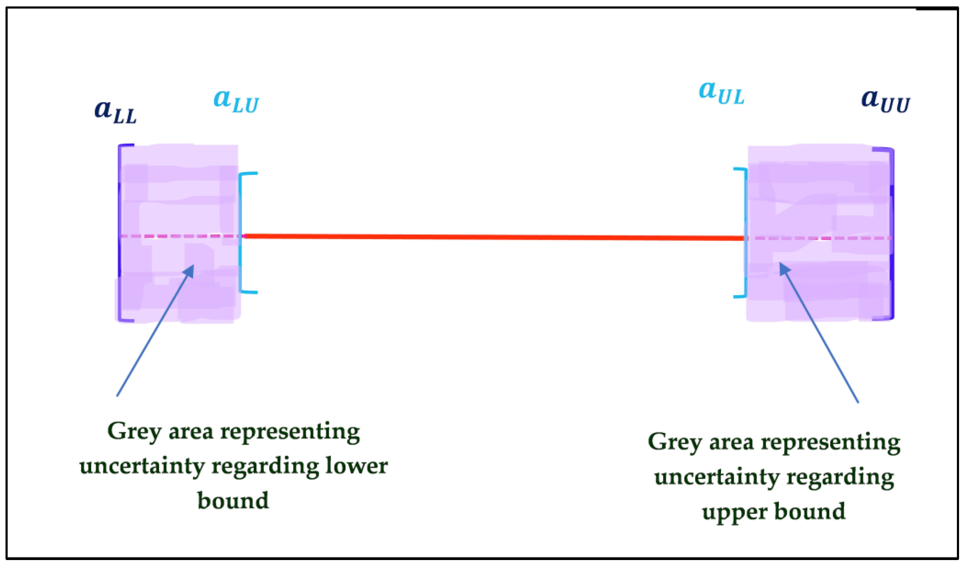
([15,16]). An interval number given by $\mathcal{A}=\left[\left[a_{LL},a_{LU}\right],\left[{ a}_{UL},a_{UU}\right]\right]$ in which $a_{LL}\le a_{LU}\le a_{UL}\le a_{UU}$ is called a T2IN.

A T2IN has uncertain upper and lower bounds. The lower and upper bounds lie in the intervals $\left[a_{LL},a_{LU}\right]$, and $\left[a_{UL},a_{UU}\right]$, respectively. As a particular case, if the upper and lower bounds lie in {$a_{LL},a_{LU}$} and {$a_{UL},a_{UU}$}, respectively, then a T2IN includes the uncertain combinations of four interval numbers, namely, $\left[a_{LL},{ a}_{UL}\right],\left[a_{LL},a_{UU}\right]$, $\left[a_{LU},{ a}_{UL}\right]$, and $\left[a_{LU},a_{UU}\right]$. Therefore, a T2IN is an uncertain combination of interval numbers. Thus, a T2IN generalizes the traditional interval numbers. Figure 1 depicts the sense of generalization in interval uncertainty made by a T2IN.

Definition 2

([15]). Let $\mathcal{A}=\left[\left[a_{LL},a_{LU}\right],\left[{ a}_{UL},a_{UU}\right]\right]$ and $\mathcal{B}=\left[\left[b_{LL},b_{LU}\right],\left[b_{UL},b_{UU}\right]\right]$ be two T2INs and $\gamma$ be any real number. Then, addition and scalar multiplication are given as

$$\begin{array}{c}\mathit{Addition}. \mathcal{A}⊞\mathcal{B}=\left[[a_{LL}+b_{LL},a_{LU}+b_{LU}],[a_{UL}+b_{UL},a_{UU}+b_{UU}]\right]\\ \mathit{Scalar}\mathit{multiplication}. \gamma ⊡\mathcal{A}=\left\{\begin{array}{c}\left[[\gamma a_{LL},\gamma a_{LU}],[\gamma a_{UL},\gamma a_{UU}]\right] for \gamma \ge 0\\ \left[[\gamma a_{UU},\gamma a_{UL}],[\gamma a_{LU},\gamma a_{LL}]\right], for \gamma <0\end{array}\right.\end{array}$$

Definition 3

([19]). The interval width of $\mathcal{A}=\left[\right[a_{LL},a_{LU}],[a_{UL},a_{UU}\left]\right]$ is defined as $\mathcal{W}\left(\mathcal{A}\right)=[a_{UL}-a_{LU}, a_{UU}-a_{LL}]$.

For example, let a T2IN be taken as $\mathcal{A}=\left[\right[\mathrm{2,3}],[\mathrm{10,11}\left]\right]$. Then, the interval width is $\left(\mathcal{A}\right)=[7, 9]$, an interval itself. A T2IN is a degenerate interval number when the bounds were crisp instead of intervals. Then, $a_{LL}=a_{LU}=a_L$, $a_{UL}=a_{UU}=a_U$, and $\mathcal{W}\left(\mathcal{A}\right)=a_U-a_L$ is the width of the interval number $[a_L,a_U]$.

Definition 4

([19]). Let $\mathcal{A}=\left[\left[a_{LL},a_{LU}\right],\left[a_{UL},a_{UU}\right]\right]$ and $\mathcal{B}=\left[\left[b_{LL},b_{LU}\right],\left[b_{UL},b_{UU}\right]\right]$ be two T2INs. Then, $\mathcal{W}\left(\mathcal{A}\right){\succcurlyeq }_{in}\mathcal{W}\left(\mathcal{B}\right)$ is equivalent to $a_{UL}-a_{LU}\ge b_{UL}-b_{UL}$ and $a_{UU}-a_{LL}\ge b_{UU}-b_{LL}$ . In that case, we say that $\mathcal{A}$ has a greater interval width than $\mathcal{B}$.

Definition 5

([15]). The generalized Hukuhara difference between two T2Ins $\mathcal{A}=\left[\right[a_{LL},a_{LU}],[a_{UL},a_{UU}\left]\right]$ and $\mathcal{B}=\left[\right[b_{LL},b_{LU}],[b_{UL},b_{UU}\left]\right]$ is defined as

$$\mathcal{A}{\boxminus }_g\mathcal{B}=\begin{array}{c}\left[\right[\mathit{min}\left\{a_{LL}-b_{LL},a_{UU}-b_{UU}\right\}, min\{a_{LU}-b_{LU},a_{UL}-b_{UL}\}],\\ [max\left\{a_{LL}-b_{LL},a_{UU}-b_{UU}\right\},\mathit{max}\{a_{LU}-b_{LU},a_{UL}-b_{UL}\}]]\end{array}$$

Lemma 1

([19]). Let $\mathcal{A}=\left[\left[a_{LL},a_{LU}\right],\left[a_{UL},a_{UU}\right]\right]$ and $\mathcal{B}=\left[\left[b_{LL},b_{LU}\right],\left[b_{UL},b_{UU}\right]\right]$ be two T2INs. Then, the generalized Hukuhara difference between them depends on interval widths as follows:

$$\mathcal{A}{\boxminus }_g\mathcal{B}=\left\{\begin{array}{c}\left[[a_{LL}-b_{LL},a_{LU}-b_{LU}],[a_{UL}-b_{UL},a_{UU}-b_{UU}]\right], when \mathcal{W}\left(\mathcal{A}\right){\succcurlyeq }_{in}\mathcal{W}\left(\mathcal{B}\right)\\ \left[[a_{UU}-b_{UU},a_{UL}-b_{UL}],[a_{LU}-b_{LU},a_{LL}-b_{LL}]\right], when \mathcal{W}\left(\mathcal{B}\right){\succcurlyeq }_{in}\mathcal{W}\left(\mathcal{A}\right)\end{array}\right.$$

3. Existence and Uniqueness of Initial Valued Differential Equations

A type-2 interval number $C=\left[\right[c_{LL},c_{LU}],[c_{UL},c_{UU}\left]\right]$ will be the generalized Hukuhara difference of $\mathcal{A}$ and $\mathcal{B}$ only if either of the following conditions is satisfied: $\mathcal{A}=\mathcal{B}⊞C$ when $\mathcal{W}\left(\mathcal{A}\right){\succcurlyeq }_{in}\mathcal{W}\left(\mathcal{B}\right)$, or $\mathcal{B}=\mathcal{A}⊞\{(-1)⊡C\}$ when $\mathcal{W}\left(\mathcal{B}\right){\succcurlyeq }_{in}\mathcal{W}\left(\mathcal{A}\right)$.

A function ${‖.‖}_4:{\mathsf{{\rm K}}}_4\to R^{+}$ defined by ${‖\mathcal{A}‖}_4=max\{\left|a_{LL}\right|,\left|a_{LU}\right|,\left|a_{UL}\right|,\left|b_{UU}\right|\}$ is the norm on the set of all type-2 interval numbers. The norm ${‖.‖}_4$ gives the metric ${\mathsf{\Delta }}_4:{\mathsf{{\rm K}}}_4\times {\mathsf{{\rm K}}}_4\to R^{+}$ defined by ${\mathsf{\Delta }}_4\left(\mathcal{A},\mathcal{B}\right)=max\left\{\left|a_{LL}-b_{LL}\right|,\left|a_{LU}-b_{LU}\right|,\left|a_{UL}-b_{UL}\right|,\left|a_{UU}-b_{UU}\right|\right\},$ for two type-2 interval numbers $\mathcal{A}=\left[\right[a_{LL},a_{LU}],[a_{UL},a_{UU}\left]\right]$ and $\mathcal{B}=\left[\right[b_{LL},b_{LU}],[b_{UL},b_{UU}\left]\right]$. The space of all type-2 interval numbers is complete under the metric ${\mathsf{\Delta }}_4$. Also, it can be shown that the metric is sequentially compact, totally bounded, and separable.

Definition 6.

A function $\mathcal{F}$ defined as $\mathcal{F}\left(\mathit{x}\right)=\left[[{\mathit{f}}_{\mathit{L}\mathit{L}}(\mathit{x}),{\mathit{f}}_{\mathit{L}\mathit{U}}(\mathit{x})],[{\mathit{f}}_{\mathit{U}\mathit{L}}\left(\mathit{x}\right),{\mathit{f}}_{\mathit{U}\mathit{U}}(\mathit{x})]\right]$, where each of ${\mathit{f}}_{\mathit{L}\mathit{L}}$, ${\mathit{f}}_{\mathit{L}\mathit{U}}$, ${\mathit{f}}_{\mathit{U}\mathit{L}}$, and ${\mathit{f}}_{\mathit{U}\mathit{U}}$ are all crisp functions maintaining the order ${\mathit{f}}_{\mathit{L}\mathit{L}}(\mathit{x})\le {\mathit{f}}_{\mathit{L}\mathit{U}}(\mathit{x})\le {\mathit{f}}_{\mathit{U}\mathit{L}}\left(\mathit{x}\right)\le {\mathit{f}}_{\mathit{U}\mathit{U}}(\mathit{x})$ throughout the domain of definitions $\mathcal{D}$ is called a T2IF on $\mathcal{D}$.

$C([a,b], {\mathsf{{\rm K}}}_4)$, the set of all type-2 interval-valued continuous functions defined on $([a,b])$, is a closed subset of $B([a,b], {\mathsf{{\rm K}}}_4)$, and hence it is a complete norm space.

Theorem 1.

Let $\mathcal{F}$ be a T2IF defined on $\left[a,b\right]$ that is given by $\mathcal{F}\left(x\right)=\left[[f_{LL}(x),{ f}_{LU}(x)],[f_{UL}\left(x\right),f_{UU}(x)]\right]$. If $\mathcal{F}$ is generalized Hukuhara differentiable and $\mathcal{W}$-monotonic on $\left[a,b\right]$ , then each of $f_{LL},{ f}_{LU}, f_{UL}, f_{UU}$ are differentiable on $\left[a,b\right]$, and furthermore:

(i) 

$\frac{d\mathcal{F}(x)}{dx}=\left[[\frac{d{f}_{LL}(x)}{dx},\frac{d{f}_{LU}(x)}{dx}],[\frac{d{f}_{UL}(x)}{dx},\frac{d{f}_{UU}(x)}{dx}]\right]$, when $\mathcal{F}$ is $\mathcal{W}$-increasing for all $x\in [a,b]$.

(ii) 

$\frac{d\mathcal{F}(x)}{dx}=\left[[\frac{d{f}_{UU}(x)}{dx},\frac{d{f}_{UL}(x)}{dx}],[\frac{d{f}_{LU}(x)}{dx},\frac{d{f}_{LL}(x)}{dx}]\right]$, when $\mathcal{F}$ is $\mathcal{W}$-decreasing for all $x\in [a,b]$.

Proof of Theorem 1.

Let $x\in \left[a,b\right]$ arbitrary and, $\mathcal{F}$ is generalized Hukuhara differentiable. That is, $\frac{d\mathcal{F}(x)}{dx}=\underset{ϵ\to 0}{\lim }\frac{\mathcal{F}\left({\mathrm{x}}_0+ϵ\right){\boxminus }_g\mathcal{F}\left({\mathrm{x}}_0\right)}{ϵ}$ exists finitely, and $\mathcal{F}$ is $\mathcal{W}$-monotone on $\left[a,b\right]$. We consider two cases as follows:

Case 1.

When $\mathcal{W}$-increasing on $\left[a,b\right]$

Since $\frac{d\mathcal{F}(x)}{dx}=\underset{ϵ\to 0}{\lim }\frac{\mathcal{F}\left(\mathrm{x}+ϵ\right){\boxminus }_g\mathcal{F}\left(\mathrm{x}\right)}{ϵ}$ exists, then $\underset{ϵ\to 0-}{\lim }\frac{\mathcal{F}\left(\mathrm{x}+ϵ\right){\boxminus }_g\mathcal{F}\left(\mathrm{x}\right)}{ϵ}=\underset{ϵ\to 0+}{\lim }\frac{\mathcal{F}\left(\mathrm{x}+ϵ\right){\boxminus }_g\mathcal{F}\left(\mathrm{x}\right)}{ϵ}$. Then, by Lemma 1, we have obtained the type-2 interval equation as follows:

$$\underset{ϵ\to 0-}{\lim }\frac{\left[\begin{array}{c}\left[f_{UU}\left(x+ϵ\right)-f_{UU}\left(x\right),f_{UL}\left(x+ϵ\right)-f_{UL}\left(x\right)\right]\\ \left[f_{LU}\left(x+ϵ\right)-f_{LU}\left(x\right),f_{LL}\left(x+ϵ\right)-f_{LL}\left(x\right)\right]\end{array},\right]}{ϵ}=\underset{ϵ\to 0+}{\lim }\frac{\left[\begin{array}{c}\left[f_{LL}\left(x+ϵ\right)-f_{LL}\left(x\right),f_{LU}\left(x+ϵ\right)-f_{LU}\left(x\right)\right]\\ \left[f_{UL}\left(x+ϵ\right)-f_{UL}\left(x\right),f_{UU}\left(x+ϵ\right)-f_{UU}\left(x\right)\right]\end{array},\right]}{ϵ}$$

The above equation leads to the consequence as follows:

$$\left[\begin{array}{c}\left[\underset{ϵ\to 0-}{\mathrm{Lim}}\frac{f_{LL}\left(x+ϵ\right)-f_{LL}\left(x\right)}{ϵ},\underset{ϵ\to 0-}{\lim }\frac{f_{LU}\left(x+ϵ\right)-f_{LU}\left(x\right)}{ϵ}\right]\\ \left[\underset{ϵ\to 0-}{\lim }\frac{f_{UL}\left(x+ϵ\right)-f_{UL}\left(x\right)}{ϵ}, \underset{ϵ\to 0-}{\lim }\frac{f_{UU}\left(x+ϵ\right)-f_{UU}\left(x\right)}{ϵ}\right]\end{array},\right]=\left[\begin{array}{c}\left[\underset{ϵ\to 0+}{\lim }\frac{f_{LL}\left(x+ϵ\right)-f_{LL}\left(x\right)}{ϵ},\underset{ϵ\to 0+}{\lim }\frac{f_{LU}\left(x+ϵ\right)-f_{LU}\left(x\right)}{ϵ}\right]\\ \left[\underset{ϵ\to 0+}{\lim }\frac{f_{UL}\left(x+ϵ\right)-f_{UL}\left(x\right)}{ϵ}, \underset{ϵ\to 0+}{\lim }\frac{f_{UU}\left(x+ϵ\right)-f_{UU}\left(x\right)}{ϵ}\right]\end{array},\right]$$

Equating components of T2IN, we conclude that each of $f_{LL},f_{LU},f_{UL},f_{UU}$ are differentiable on $x\in \left[a,b\right]$, and in that case, $\frac{d\mathcal{F}\left(x\right)}{dx}=\left[\left[\frac{d{f}_{LL}\left(x\right)}{dx},\frac{d{f}_{LU}\left(x\right)}{dx}\right],\left[\frac{d{f}_{UL}\left(x\right)}{dx},\frac{d{f}_{UU}\left(x\right)}{dx}\right]\right]$.

Case 2.

When $\mathcal{W}$-decreasing on $\left[a,b\right]$

Since $\frac{d\mathcal{F}(x)}{dx}=\underset{ϵ\to 0}{\lim }\frac{\mathcal{F}\left(\mathrm{x}+ϵ\right){\boxminus }_g\mathcal{F}\left(\mathrm{x}\right)}{ϵ}$ exists, then $\underset{ϵ\to 0-}{\lim }\frac{\mathcal{F}\left(\mathrm{x}+ϵ\right){\boxminus }_g\mathcal{F}\left(\mathrm{x}\right)}{ϵ}=\underset{ϵ\to 0+}{\lim }\frac{\mathcal{F}\left(\mathrm{x}+ϵ\right){\boxminus }_g\mathcal{F}\left(\mathrm{x}\right)}{ϵ}$.

Then, by Lemma 1, we have obtained the type-2 interval equation as follows:

$$\underset{ϵ\to 0-}{\lim }\frac{\left[\begin{array}{c}\left[f_{LL}\left(x+ϵ\right)-f_{LL}\left(x\right),f_{LU}\left(x+ϵ\right)-f_{LU}\left(x\right)\right]\\ \left[f_{UL}\left(x+ϵ\right)-f_{UL}\left(x\right),f_{UU}\left(x+ϵ\right)-f_{UU}\left(x\right)\right]\end{array},\right]}{ϵ}=\underset{ϵ\to 0+}{\lim }\frac{\left[\begin{array}{c}\left[f_{UU}\left(x+ϵ\right)-f_{UU}\left(x\right),f_{UL}\left(x+ϵ\right)-f_{UL}\left(x\right)\right]\\ \left[f_{LU}\left(x+ϵ\right)-f_{LU}\left(x\right),f_{LL}\left(x+ϵ\right)-f_{LL}\left(x\right)\right]\end{array},\right]}{ϵ}$$

The above equation leads to the consequence as follows:

$$\left[\begin{array}{c}\left[\underset{ϵ\to 0-}{\lim }\frac{f_{UU}\left(x+ϵ\right)-f_{UU}\left(x\right)}{ϵ},\underset{ϵ\to 0-}{\lim }\frac{f_{UL}\left(x+ϵ\right)-f_{UL}\left(x\right)}{ϵ}\right]\\ \left[\underset{ϵ\to 0-}{\lim }\frac{f_{LU}\left(x+ϵ\right)-f_{LU}\left(x\right)}{ϵ}, \underset{ϵ\to 0-}{\lim }\frac{f_{LL}\left(x+ϵ\right)-f_{LL}\left(x\right)}{ϵ}\right]\end{array},\right]=\left[\begin{array}{c}\left[\underset{ϵ\to 0+}{\lim }\frac{f_{UU}\left(x+ϵ\right)-f_{UU}\left(x\right)}{ϵ},\underset{ϵ\to 0+}{\lim }\frac{f_{UL}\left(x+ϵ\right)-f_{UL}\left(x\right)}{ϵ}\right]\\ \left[\underset{ϵ\to 0+}{\lim }\frac{f_{LU}\left(x+ϵ\right)-f_{LU}\left(x\right)}{ϵ}, \underset{ϵ\to 0+}{\lim }\frac{f_{LL}\left(x+ϵ\right)-f_{LL}\left(x\right)}{ϵ}\right]\end{array},\right]$$

Equating components of T2IN, we conclude that each of $f_{LL},f_{LU},f_{UL},f_{UU}$ are differentiable on $x\in \left[a,b\right]$, and in that case, $\frac{d\mathcal{F}(x)}{dx}=\left[[\frac{d{f}_{UU}(x)}{dx},\frac{d{f}_{UL}(x)}{dx}],[\frac{d{f}_{LU}(x)}{dx},\frac{d{f}_{LL}(x)}{dx}]\right]$. □

Definition 7.

Let $\mathcal{F}$ be a T2IF defined on $[a,b]$ given by $\mathcal{F}\left(x\right)=\left[[f_{LL}(x),f_{LU}(x)],[f_{UL}\left(x\right),f_{UU}(x)]\right]$. Then, $\mathcal{F}$ is Riemann integrable on $[a,b]$ when $f_{LL},{ f}_{LU}, f_{UL},$ and $f_{UU}$ are all Riemann integrable functions on $[a,b]$. In that case, we define the Riemann integration of the T2IF $\mathcal{F}$ as follows:

$${\int }_a^b\mathcal{F}\left(x\right)dx=[[{\int }_a^b{f}_{LL}\left(x\right)dx,{\int }_a^b{f}_{LU}\left(x\right)dx],[{\int }_a^b{f}_{UL}\left(x\right)dx,{\int }_a^b{f}_{UU}\left(x\right)dx]]$$

Now, we introduce the existence and uniqueness of solvability of the differential equation in a type-2 interval environment.

Let us consider a type-2 interval-valued differential equation of first order given as

$$\left\{\begin{array}{c}\frac{d\widetilde{y_2}}{dx}=\widetilde{{\mathsf{Ϝ}}_2}(x, \widetilde{y_2}(x))\\ \widetilde{y_2}(x_0)=\widetilde{y_{02}}\end{array}\right.$$

(1)

In Equation (1), $\widetilde{{\mathit{y}}_{\mathbf{2}}}$ is a type-2 valued dependent variable while $\mathit{x}$ is a crisp independent variable.

In the system given by Equation (1), $\widetilde{{\mathbf{F}}_{\mathbf{2}}}:[\mathit{a},\mathit{b}]\times {\mathit{I}}_{\mathbf{2}}\to {\mathit{I}}_{\mathbf{2}}$ is a type-2 interval-valued function (where ${\mathit{I}}_{\mathbf{2}}$ is the set of all type-2 interval numbers), which is given by four components as follows:

$$\widetilde{{\mathsf{Ϝ}}_2}(x, \widetilde{y_2}(x))=\left[\right[f_{LL}(x, \widetilde{y_2}(x)), f_{LU}(x, \widetilde{y_2}(x))],[f_{UL}(x, \widetilde{y_2}(x)), f_{UU}(x, \widetilde{y_2}(x))\left]\right]$$

Also, the dependent variable $\widetilde{{\mathit{y}}_{\mathbf{2}}}$ and initial value $\widetilde{{\mathit{y}}_{\mathbf{02}}}$ are given respectively as $\widetilde{{\mathit{y}}_{\mathbf{2}}}(\mathit{x})=\left[\right[{\mathit{y}}_{\mathit{L}\mathit{L}}(\mathit{x},\widetilde{{\mathit{y}}_{\mathbf{2}}}),{\mathit{y}}_{\mathit{L}\mathit{U}}(\mathit{x},\widetilde{{\mathit{y}}_{\mathbf{2}}})],[{\mathit{y}}_{\mathit{U}\mathit{L}}(\mathit{x},\widetilde{{\mathit{y}}_{\mathbf{2}}}),{\mathit{y}}_{\mathit{U}\mathit{U}}(\mathit{x},\widetilde{{\mathit{y}}_{\mathbf{2}}})\left]\right]$ and $\widetilde{{\mathit{y}}_{\mathbf{02}}}=\left[\right[{\mathit{y}}_{\mathbf{0}\mathit{L}\mathit{L}},{\mathit{y}}_{\mathbf{0}\mathit{L}\mathit{U}}],[{\mathit{y}}_{\mathbf{0}\mathit{U}\mathit{L}},{\mathit{y}}_{0\mathit{U}\mathit{U}}\left]\right]$. In Equation (1), $\frac{\mathit{d}\widetilde{{\mathit{y}}_{\mathbf{2}}}}{\mathit{d}\mathit{x}}$ represents the generalized Hukuhara differentiability of the type-2 valued dependent variable $\widetilde{{\mathit{y}}_{\mathbf{2}}}$ concerning x, the crisp independent variable.

Now, Equation (1) is equivalent to the integral equation

$$\widetilde{y_2}(x){\boxminus }_{gH}\widetilde{y_{02}}={\int }_{x_0}^x\widetilde{{\mathsf{Ϝ}}_2}(u, \widetilde{y_2}(u))du.$$

(2)

Using the sense of the generalized Hukuhara difference of a type-2 interval-valued function, Equation (2) is equivalent to either

$$\widetilde{y_2}(x)=\widetilde{y_{02}}⊞{\int }_{x_0}^x\widetilde{{\mathsf{Ϝ}}_2}(u, \widetilde{y_2}(u))du$$

(3)

$$\mathrm{Or}, \widetilde{y_{02}}=\widetilde{y_2}(x)⊞(-1)\odot {\int }_{x_0}^x\widetilde{{\mathsf{Ϝ}}_2}(u, \widetilde{y_2}(u))du$$

(4)

Theorem 2.

We define a closed ball in type-2 interval-valued functions as follows:

$$\overline{{\mathit{B}}_{\mathit{r}}}(\widetilde{{\mathit{y}}_{\mathbf{02}}})=\left\{\widetilde{{\mathit{z}}_{\mathbf{2}}}\in {\mathit{I}}_{\mathbf{2}}:{\mathit{\mu }}_{\mathbf{2}}(\widetilde{{\mathit{z}}_{\mathbf{2}}},\widetilde{{\mathit{y}}_{\mathbf{02}}})\right.\le \mathit{r}$$

where ${\mathit{\mu }}_{\mathbf{2}}$ is the type-2 interval numbers metric and $\mathit{r}$ is a positive real number. In the above definition, $\overline{{\mathit{B}}_{\mathit{r}}}(\widetilde{{\mathit{y}}_{\mathbf{02}}})$ is the closed ball having a radius $\mathit{r}$ and a center at $\widetilde{{\mathit{y}}_{\mathbf{02}}}$. Then, we construct a region ${\mathit{R}}^{\mathit{*}}$ as follows: ${\mathit{R}}^{\mathit{*}}=[{\mathit{x}}_{\mathbf{0}},{\mathit{x}}_{\mathbf{0}}+\mathit{h}]\times \overline{{\mathit{B}}_{\mathit{r}}}(\widetilde{{\mathit{y}}_{\mathbf{02}}})$, where ${\mathit{x}}_{\mathbf{0}},\mathit{h}$ are crisp numbers and $\widetilde{{\mathit{y}}_{\mathbf{02}}}$ is a type-2 interval number. Then, we construct $\widetilde{{\mathbf{F}}_{\mathbf{2}}}:{\mathit{R}}^{\mathit{*}}\to {\mathit{I}}_{\mathbf{2}}$ as a continuous, non-trivial type-2 valued function, which satisfies the Lipschitz condition as follows:

$${\mathit{\mu }}_{\mathbf{2}}(\widetilde{{\mathbf{F}}_{\mathbf{2}}}(\mathit{x},\widetilde{{\mathit{y}}_{\mathbf{2}}}(\mathit{x})),\widetilde{{\mathbf{F}}_{\mathbf{2}}}(\mathit{x},\widetilde{{\mathit{z}}_{\mathbf{2}}}(\mathit{x})))\le \mathit{k}{\mathit{\mu }}_{\mathbf{2}}(\widetilde{{\mathit{y}}_{\mathbf{2}}}(\mathit{x}),\widetilde{{\mathit{z}}_{\mathbf{2}}}(\mathit{x}))$$

(5)

for all $(x, \widetilde{y_2}(x)), (x, \widetilde{z_2}(x))$ in $R^{*}$.

Then, the system given by Equation (1) has two unique solutions, ${\widetilde{{\mathit{y}}_{\mathbf{2}}}}^{\mathbf{1}}$ and ${\widetilde{{\mathit{y}}_{\mathbf{2}}}}^{\mathbf{2}}$ , provided by the successive iterations as follows:

$$\left\{\begin{array}{c}{\widetilde{y_{(n+1), 2}}}^1(x)=\widetilde{y_{02}}⊞{\int }_{x_0}^x\widetilde{{\mathsf{Ϝ}}_2}(u, {\widetilde{y_{n, 2}}}^1(u))du\\ \widetilde{y_{02}}={\widetilde{y_{(n+1), 2}}}^2(x)⊞(-1)\odot {\int }_{x_0}^x\widetilde{{\mathsf{Ϝ}}_2}(u, {\widetilde{y_{n, 2}}}^2(u))du\end{array}\right.$$

(6)

Proof of Theorem 2.

It is perceived that Equation (1) is equivalent to either Equation (3) or Equation (4).

Since $I_2$, the space of all type-2 interval numbers form a metric space under the metric ${\mu }_2$, ($I_2, {\mu }_2$) is a metric Hausdroff space and is therefore locally compact. Therefore, $\overline{B_r}(\widetilde{y_{02}})$ is compact. Then, $f_{UL}-f_{LU}$ and $f_{UU}-f_{LL}$ are bounded functions defined on $R^{*}$. Thus, positive real numbers $M_1$ and $M_2$ exist such that the following are true:

$$\left\{\begin{array}{c}{(f}_{UL}-f_{LU})(x, \widetilde{y_2})\le M_1\\ {(f}_{UU}-f_{LL})(x, \widetilde{y_2})\le M_2\end{array}\right.$$

(7)

Therefore, the interval width of $\widetilde{{\mathbf{F}}_2}$ satisfies the following inequalities:

$$\mathcal{W}\left(\widetilde{{\mathsf{Ϝ}}_2}(x, \widetilde{y_2}(x))\right){\le }_{in}[M_1, M_2]$$

(8)

Since $\widetilde{y_{02}}$ is a non-trivial type-2 interval number, $\mathcal{W}\left(\widetilde{y_{02}}\right){\succcurlyeq }_{in}[0,0]$. That is, ${(y}_{0UL}-y_{0LU})\ge 0$ and ${(y}_{0UU}-y_{0LL})\ge 0$. Let $h_1=min\{h,\frac{{(y}_{0UL}-y_{0LU})}{M_1},\frac{{(y}_{0UU}-y_{0LL})}{M_2}\}$. Now, negation of ${\int }_{x_0}^x\widetilde{{\mathsf{Ϝ}}_2}(u,\widetilde{y_2}(u))du$ can be obtained as follows:

$$\begin{array}{l}(-1)\odot {\int }_{x_0}^x\widetilde{{\mathsf{Ϝ}}_2}(u, \widetilde{y_2}(u))du\\ =\left[\right[-{\int }_{x_0}^x{f}_{UU}(u, \widetilde{y_2}(u))du,-{\int }_{x_0}^x{f}_{UL}(u, \widetilde{y_2}(u))du],[-{\int }_{x_0}^x{f}_{LU}(u, \widetilde{y_2}(u))du,-{\int }_{x_0}^x{f}_{LL}(u, \widetilde{y_2}(u))du\left]\right]\end{array}$$

Therefore, the interval width representation of the above equation can be obtained as follows:

$$\mathcal{W}\left((-1)\odot {\int }_{x_0}^x\widetilde{{\mathsf{Ϝ}}_2}(u, \widetilde{y_2}(u))du\right)=\left[{\int }_{x_0}^x\left(f_{UU}-f_{LL}\right)\left(u, \widetilde{y_2}\left(u\right)\right)du, {\int }_{x_0}^x\left(f_{UL}-f_{LU}\right)\left(u, \widetilde{y_2}\left(u\right)\right)du\right]$$

$${\le }_{in}[M_1, M_2](x-x_0) {\le }_{in}[M_1{h}_1, M_2{h}_1]{\le }_{in}[{(y}_{0UL}-y_{0LU}), {(y}_{0UU}-y_{0LL})]=\mathcal{W}\left(\widetilde{y_{02}}\right)$$

$$\mathrm{That} \mathrm{is}, \mathcal{W}\left((-1)\odot {\int }_{x_0}^x\widetilde{{\mathsf{Ϝ}}_2}(u, \widetilde{y_2}(u))du\right){\le }_{in}\mathcal{W}\left(\widetilde{y_{02}}\right)$$

(9)

Therefore, the Hukuhara difference $\widetilde{y_{02}}{\boxminus }_H(-1)\odot {\int }_{x_0}^x\widetilde{{\mathsf{Ϝ}}_2}(u,\widetilde{y_2}(u))du$ exists.

We construct $C_0=[x_0, x_0+h_1]\times \overline{B_r}(\widetilde{y_{02}})$, a compact set. Then, we consider two operations, $\mathsf{\Phi }$ and $\mathsf{\Psi }$, as follows:

$$\left\{\begin{array}{c}\mathsf{\Phi }(\widetilde{y_2}(x_0))=\mathsf{\Psi }(\widetilde{y_2}(x_0))=\widetilde{y_{02}}\\ \mathsf{\Phi }(\widetilde{y_2}(x))=\widetilde{y_{02}}⊞{\int }_{x_0}^x\widetilde{{\mathsf{Ϝ}}_2}(u, \widetilde{y_2}(u))du\\ \mathsf{\Psi }(\widetilde{y_2}(x))=\widetilde{y_{02}}{\boxminus }_H(-1)\odot {\int }_{x_0}^x\widetilde{{\mathsf{Ϝ}}_2}(u, \widetilde{y_2}(u))du\end{array}\right.$$

(10)

In System (10), the operator $\mathsf{\Phi }$ is well-defined irrespective of the choice of the neighborhood of $x_0.$ But, $\mathsf{\Psi }$ is well-defined depending on the choice of the neighborhood of $x_0$. Now, by the metric space property, we have the following results:

$${\mu }_2\left(\mathsf{\Phi }\left(\widetilde{y_2}\left(x\right)\right),\widetilde{y_{02}}\right)={\mu }_2\left(\widetilde{y_{02}}⊞{\int }_{x_0}^x\widetilde{{\mathsf{Ϝ}}_2}\left(u,\widetilde{y_2}\left(u\right)\right)du,\widetilde{y_{02}}\right)$$

$$={\mu }_2({\int }_{x_0}^x\widetilde{{\mathsf{Ϝ}}_2}(u, \widetilde{y_2}(u))du, 0)\le {\int }_{x_0}^x{\mu }_2(\widetilde{{\mathsf{Ϝ}}_2}(u, \widetilde{y_2}(u)),0)du\le M_3(x-x_0)$$

(11)

The above result is obtained as $\widetilde{{\mathsf{Ϝ}}_{\mathbf{2}}}$, which is a continuous function on the compact set ${\mathit{C}}_{\mathbf{0}}$. Again,

$${\mu }_2\left(\mathsf{\Psi }\left(\widetilde{y_2}\left(x\right)\right),\widetilde{y_{02}}\right)={\mu }_2\left(\widetilde{y_{02}}{\boxminus }_H\left(-1\right)\odot {\int }_{x_0}^x\widetilde{{\mathsf{Ϝ}}_2}\left(u,\widetilde{y_2}\left(u\right)\right)du,\widetilde{y_{02}}\right)$$

$$={\mu }_2({\int }_{x_0}^x\widetilde{{\mathsf{Ϝ}}_2}(u, \widetilde{y_2}(u))du, 0)\le {\int }_{x_0}^x{\mu }_2(\widetilde{{\mathsf{Ϝ}}_2}(u, \widetilde{y_2}(u)),0)du\le M_3(x-x_0)$$

(12)

Next, we consider $h_2=min\{min\{h,\frac{{(y}_{0UL}-y_{0LU})}{M_1},\frac{{(y}_{0UU}-y_{0LL})}{M_2}\},\frac{r}{M_3}\}$, and we construct $C_1=[x_0,x_0+h_2]\times \overline{B_r}(\widetilde{y_{02}})$. We consider all the continuous functions from $C_1$ to $\overline{{\mathit{B}}_{\mathit{r}}}(\widetilde{{\mathit{y}}_{\mathbf{02}}})$. All such functions are complete under the sup metric for type-2 interval-valued functions.

Let $\widetilde{y_2}$ and $\widetilde{z_2}$ be two such continuous functions defined on $C_1$. Then, the following inequalities are obtained:

$$\mathrm{Then}, {\mu }_2\left(\mathsf{\Phi }\left(\widetilde{y_2}\left(x\right)\right),\mathsf{\Phi }\left(\widetilde{z_2}\left(x\right)\right)\right)$$

$$={\mu }_2\left(\widetilde{y_{02}}⊞{\int }_{x_0}^x\widetilde{{\mathsf{Ϝ}}_2}\left(u,\widetilde{y_2}\left(u\right)\right)du,\widetilde{y_{02}}⊞{\int }_{x_0}^x\widetilde{{\mathsf{Ϝ}}_2}\left(u,\widetilde{z_2}\left(u\right)\right)du\right)$$

$$={\mu }_2\left({\int }_{x_0}^x\widetilde{{\mathsf{Ϝ}}_2}\left(u,\widetilde{y_2}\left(u\right)\right)du,{\int }_{x_0}^x\widetilde{{\mathsf{Ϝ}}_2}\left(u,\widetilde{z_2}\left(u\right)\right)du\right)$$

$$\le {\int }_{x_0}^x{\mu }_2(\widetilde{{\mathsf{Ϝ}}_2}\left(u,\widetilde{y_2}\left(u\right)\right),\widetilde{{\mathsf{Ϝ}}_2}\left(u,\widetilde{z_2}\left(u\right)\right))du$$

$$\le k{\int }_{x_0}^x{\mu }_2(\widetilde{y_2}\left(u\right),\widetilde{z_2}\left(u\right))du$$

$$\le k{\int }_{x_0}^x\underset{u\in [x_0,{\mathit{x}}_0+h_2]}{\max }{\mu }_2(\widetilde{y_2}\left(u\right),\widetilde{z_2}\left(u\right))du$$

$$\le k(x-x_0){\mu }_{2, sup}(\widetilde{y_2},\widetilde{z_2})$$

And similarly, ${\mu }_2\left(\mathsf{\Psi }\left(\widetilde{y_2}\left(x\right)\right),\mathsf{\Psi }\left(\widetilde{z_2}\left(x\right)\right)\right)\le k(x-x_0){\mu }_{2,sup}(\widetilde{y_2},\widetilde{z_2})$.

If we take, $h_3<min\{min\{min\{h,\frac{{(y}_{0UL}-y_{0LU})}{M_1},\frac{{(y}_{0UU}-y_{0LL})}{M_2}\},\frac{r}{M_3}\},\frac{1}{k}\}$, then $k(x-x_0)<1$. Therefore, both $\mathsf{\Phi }$ and $\mathsf{\Psi }$ become contractions. Since Φ is a contraction, by the Banach fixed-point theorem, $\mathsf{\Phi }$ has a unique fixed point ${\widetilde{y_2}}^1$, which can be obtained by Picard’s successive iterations on the process $\mathsf{\Phi }$ and, hence,

$${\widetilde{y_{(n+1), 2}}}^1(x)=\widetilde{y_{02}}⊞{\int }_{x_0}^x\widetilde{{\mathsf{Ϝ}}_2}(u, {\widetilde{y_{n, 2}}}^1(u))du$$

Also, $\mathsf{\Psi }$ is a contraction; thus, by the Banach fixed-point theorem, $\mathsf{\Psi }$ has a unique fixed point ${\widetilde{y_2}}^2$, which can be obtained by Picard’s successive iterations on the process $\mathsf{\Psi }$ and, hence,

$${\widetilde{y_{(n+1), 2}}}^2(x)=\stackrel{~}{\widetilde{y_{02}}{\boxminus }_H\left(-1\right)\odot {\int }_{x_0}^x\widetilde{{\mathsf{Ϝ}}_2}\left(u,\widetilde{y_2}\left(u\right)\right)du}$$

Or equivalently,

$$\widetilde{y_{02}}={\widetilde{y_{(n+1), 2}}}^2(x)⊞(-1)\odot {\int }_{x_0}^x\widetilde{{\mathsf{Ϝ}}_2}(u, {\widetilde{y_{n, 2}}}^2(u))du$$

This completes the proof with the conclusion that Equation (1) has two unique solutions, which can be uniquely obtained by Equation (6), provided certain conditions hold. □

Remark 1.

This section ends with the proof of the theorem addressing the existence and uniqueness criteria for solving the differential equation in a type-2 interval environment. The succeeding section thus provides a detailed solution approach in different cases.

4. Solutions of First-Order Linear Differential Equations in Type-2 Interval Environment

A first-order linear non-homogenous differential equation in a type-2 interval environment can be represented as follows:

$$\left\{\begin{array}{c}\frac{d\widetilde{y_2}}{dx}=\widetilde{k_2}⨀\widetilde{y_2}⊞\widetilde{M_2}\\ \widetilde{y_2}(0)=\widetilde{y_{02}}\end{array}\right.$$

(13)

The preceding text ensures the existence of the solution. Here, we consider the following two cases depending upon the generalized Hukuhara differentiability of the type-2 interval-valued dependent variable $\widetilde{y_2}$.

Case 1.

When $\widetilde{y_2}$ is generalized Hukuhara differentiable of the first type

In this case, we consider four subcases concerning the signs of the type-2 interval numbers $\widetilde{k_2}$ and $\widetilde{M_2}$.

Subcase 1.1. When both $\widetilde{k_2}$ and $\widetilde{M_2}$ are positive type-2 interval numbers

In this scenario, the type-2 interval-valued differential equation in System (13) can be replaced by the equation incorporating four components as follows:

$$\left[\left[\frac{d{y}_{LL}}{dx}, \frac{d{y}_{LU}}{dx}\right],\left[\frac{d{y}_{UL}}{dx}, \frac{d{y}_{UU}}{dx}\right]\right]=\left[\left[k_{LL}{y}_{LL}+M_{LL}, k_{LU}{y}_{LU}+M_{LU}\right],\left[k_{UL}{y}_{UL}+M_{UL}, k_{UU}{y}_{UU}+M_{UU}\right]\right]$$

This gives four differential equations, which are given below.

$$\left\{\begin{array}{c}\begin{array}{c}\frac{d{y}_{LL}}{dx}=k_{LL}{y}_{LL}+M_{LL}\\ \frac{d{y}_{LU}}{dx}=k_{LU}{y}_{LU}+M_{LU}\end{array}\\ \begin{array}{c}\frac{d{y}_{UL}}{dx}=k_{UL}{y}_{UL}+M_{UL}\\ \frac{d{y}_{UU}}{dx}=k_{UU}{y}_{UU}+M_{UU}\end{array}\end{array}\right.$$

(14)

By solving the first equation in System (14), we obtain

$$y_{LL}{e}^{-k_{LL}x}=-\frac{M_{LL}}{k_{LL}}{e}^{-k_{LL}x}+c_1$$

The initial condition $\widetilde{y_2}(0)=\widetilde{y_{02}}$ compromises the crisp component $y_{LL}\left(0\right)=y_{0LL}$, which provides the value of the integrating constant as $c_1=y_{0LL}+\frac{M_{LL}}{k_{LL}}$. Hence, the first component of the type-2 interval-valued solution is obtained as follows:

$$y_{LL}=\frac{M_{LL}}{k_{LL}}\left(e^{k_{LL}x}-1\right)+y_{0LL}{e}^{k_{LL}x}$$

Similarly, the remaining components of the type-2 interval-valued solution are obtained as follows:

$$y_{LU}=\frac{M_{LU}}{k_{LU}}\left(e^{k_{LU}x}-1\right)+y_{0LU}{e}^{k_{LU}x}$$

$$y_{UL}=\frac{M_{UL}}{k_{UL}}\left(e^{k_{UL}x}-1\right)+y_{0UL}{e}^{k_{UL}x}$$

$$y_{UU}=\frac{M_{UU}}{k_{UU}}\left(e^{k_{UU}x}-1\right)+y_{0UU}{e}^{k_{UU}x}$$

Subcase 1.2. When $\widetilde{k_2}$ and $\widetilde{M_2}$ are positive and negative type-2 interval numbers, respectively

In this scenario, the type-2 interval-valued differential equation in System (13) can be replaced by the equation incorporating four components as follows:

$$\left[\left[\frac{d{y}_{LL}}{dx}, \frac{d{y}_{LU}}{dx}\right],\left[\frac{d{y}_{UL}}{dx}, \frac{d{y}_{UU}}{dx}\right]\right]=\left[\right[k_{LL}{y}_{LL}-M_{UU}, k_{LU}{y}_{LU}-M_{UL}],[k_{UL}{y}_{UL}-M_{LU}, k_{UU}{y}_{UU}-M_{LL}\left]\right]$$

This gives four differential equations, which are given below,

$$\left\{\begin{array}{c}\begin{array}{c}\frac{d{y}_{LL}}{dx}=k_{LL}{y}_{LL}-M_{UU}\\ \frac{d{y}_{LU}}{dx}=k_{LU}{y}_{LU}-M_{UL}\end{array}\\ \begin{array}{c}\frac{d{y}_{UL}}{dx}=k_{UL}{y}_{UL}-M_{LU}\\ \frac{d{y}_{UU}}{dx}=k_{UU}{y}_{UU}-M_{LL}\end{array}\end{array}\right.$$

(15)

Following the process detailed in the preceding Subcase 1.1, the four components of the solution are obtained as follows:

$$y_{LL}=\frac{M_{UU}}{k_{LL}}\left(1-e^{k_{LL}x}\right)+y_{0LL}{e}^{k_{LL}x}$$

$$y_{LU}=\frac{M_{UL}}{k_{LU}}\left(1-e^{k_{LU}x}\right)+y_{0LU}{e}^{k_{LU}x}$$

$$y_{UL}=\frac{M_{LU}}{k_{UL}}\left(1-e^{k_{UL}x}\right)+y_{0UL}{e}^{k_{UL}x}$$

$$y_{UU}=\frac{M_{LL}}{k_{UU}}\left(1-e^{k_{UU}x}\right)+y_{0UU}{e}^{k_{UU}x}$$

Subcase 1.3. When $\widetilde{k_2}$ and $\widetilde{M_2}$ are negative and positive type-2 interval numbers, respectively

In this scenario, the type-2 interval-valued differential equation in System (13) can be replaced by the equation incorporating four components as follows:

$$\left[\left[\frac{d{y}_{LL}}{dx}, \frac{d{y}_{LU}}{dx}\right],\left[\frac{d{y}_{UL}}{dx}, \frac{d{y}_{UU}}{dx}\right]\right]=\left[\right[-k_{UU}{y}_{UU}+M_{LL},-k_{UL}{y}_{UL}+M_{LU}],[-k_{LU}{y}_{LU}+M_{UL},-k_{LL}{y}_{LL}+M_{UU}\left]\right]$$

This gives four differential equations, which are given below,

$$\frac{d{y}_{LL}}{dx}=-k_{UU}{y}_{UU}+M_{LL}$$

(16)

$$\frac{d{y}_{LU}}{dx}=-k_{UL}{y}_{UL}+M_{LU}$$

(17)

$$\frac{d{y}_{UL}}{dx}=-k_{LU}{y}_{LU}+M_{UL}$$

(18)

$$\frac{d{y}_{UU}}{dx}=-k_{LL}{y}_{LL}+M_{UU}$$

(19)

From Equations (16) and (19) of the above system, we obtain

$$\frac{d^2{y}_{LL}}{d{x}^2}=-k_{UU}\frac{d{y}_{UU}}{dx}$$

$$\frac{d^2{y}_{LL}}{d{x}^2}=-k_{UU}\left[-k_{LL}{y}_{LL}+M_{UU}\right]$$

$$\frac{d^2{y}_{LL}}{d{x}^2}-k_{LL}{k}_{UU}{y}_{LL}=-k_{UU}{M}_{UU}$$

Therefore, the solution is

$$y_{LL}\left(x\right)=c_3{e}^{\sqrt{k_{LL}{k}_{UU}}x}+c_4{e}^{-\sqrt{k_{LL}{k}_{UU}}x}+\frac{1}{D^2-k_{LL}{k}_{UU}}\left(-k_{UU}{M}_{UU}\right)$$

$$y_{LL}\left(x\right)=c_3{e}^{\sqrt{k_{LL}{k}_{UU}}x}+c_4{e}^{-\sqrt{k_{LL}{k}_{UU}}x}+\frac{M_{UU}}{k_{LL}}$$

(20)

Using Equation (20) in Equation (16) and find the value of $y_{UU}\left(x\right)$ as follows:

$$y_{UU}\left(x\right)=\frac{1}{k_{UU}}\left[M_{LL}-\sqrt{k_{LL}{k}_{UU}}\left(c_3{e}^{\sqrt{k_{LL}{k}_{UU}}x}-c_4{e}^{-\sqrt{k_{LL}{k}_{UU}}x}\right)\right]$$

(21)

Using the initial conditions $y_{LL}\left(0\right)=y_{0LL}$ and $y_{UU}\left(0\right)=y_{0UU}$ in Equations (20) and (21), we obtain $c_3+c_4=y_{0LL}-\frac{M_{UU}}{k_{LL}}$ and $c_3-c_4=\frac{M_{LL}-k_{UU}{y}_{0UU}}{\sqrt{k_{LL}{k}_{UU}}}=-\left(y_{0UU}-\frac{M_{LL}}{k_{UU}}\right)\sqrt{\frac{k_{UU}}{k_{LL}}}$. Therefore, the values of the integrating constants are obtained as follows:

$$c_3=\frac{1}{2}\left[\left(y_{0LL}-\frac{M_{UU}}{k_{LL}}\right)-\left(y_{0UU}-\frac{M_{LL}}{k_{UU}}\right)\sqrt{\frac{k_{UU}}{k_{LL}}}\right]$$

$$c_4=\frac{1}{2}\left[\left(y_{0LL}-\frac{M_{UU}}{k_{LL}}\right)+\left(y_{0UU}-\frac{M_{LL}}{k_{UU}}\right)\sqrt{\frac{k_{UU}}{k_{LL}}}\right]$$

Therefore, the solutions of the crisp differential Equations (16) and (19) can be obtained as follows:

$$\begin{array}{c}{y}_{LL}\left(x\right)=\left(y_{0LL}-\frac{M_{UU}}{k_{LL}}\right)\cosh \left(\sqrt{k_{LL}{k}_{UU}}x\right)-\left(y_{0UU}-\frac{M_{LL}}{k_{UU}}\right)\sqrt{\frac{k_{UU}}{k_{LL}}}\sinh \left(\sqrt{k_{LL}{k}_{UU}}x\right)+\frac{M_{UU}}{k_{LL}}\\ y_{UU}\left(x\right)=\left(y_{0UU}-\frac{M_{LL}}{k_{UU}}\right)\cosh \left(\sqrt{k_{LL}{k}_{UU}}x\right)-\left(y_{0LL}-\frac{M_{UU}}{k_{LL}}\right)\sqrt{\frac{k_{LL}}{k_{UU}}}\sinh \left(\sqrt{k_{LL}{k}_{UU}}x\right)+\frac{M_{LL}}{k_{UU}}\end{array}$$

Similarly, by solving the crisp differential Equations (17) and (18), we obtain the following results:

$$y_{LU}\left(x\right)=\left(y_{0LU}-\frac{M_{UL}}{k_{LU}}\right)\cosh \left(\sqrt{k_{LU}{k}_{UL}}x\right)-\left(y_{0UL}-\frac{M_{LU}}{k_{UL}}\right)\sqrt{\frac{k_{UL}}{k_{LU}}}\sinh \left(\sqrt{k_{LU}{k}_{UL}}x\right)+\frac{M_{UL}}{k_{LU}}$$

$$y_{UL}\left(x\right)=\left(y_{0UL}-\frac{M_{LU}}{k_{UL}}\right)\cosh \left(\sqrt{k_{LU}{k}_{UL}}x\right)-\left(y_{0LU}-\frac{M_{UL}}{k_{LU}}\right)\sqrt{\frac{k_{LU}}{k_{UL}}}\sinh \left(\sqrt{k_{LU}{k}_{UL}}x\right)+\frac{M_{LU}}{k_{UL}}$$

Subcase 1.4. When both $\widetilde{k_2}$ and $\widetilde{M_2}$ are negative type-2 interval numbers

In this scenario, the type-2 interval-valued differential equation in System (13) can be replaced by the equation incorporating four components as follows:

$$\left[\right[\frac{d{y}_{LL}}{dx}, \frac{d{y}_{LU}}{dx}],[\frac{d{y}_{UL}}{dx}, \frac{d{y}_{UU}}{dx}\left]\right]=\left[\right[-k_{UU}{y}_{UU}-M_{UU},-k_{UL}{y}_{UL}-M_{UL}],[-k_{LU}{y}_{LU}-M_{LU},-k_{LL}{y}_{LL}-M_{LL}\left]\right]$$

This gives four differential equations, which are given below,

$$\frac{d{y}_{LL}}{dx}=-k_{UU}{y}_{UU}-M_{UU}$$

(22)

$$\frac{d{y}_{LU}}{dx}=-k_{UL}{y}_{UL}-M_{UL}$$

(23)

$$\frac{d{y}_{UL}}{dx}=-k_{LU}{y}_{LU}-M_{LU}$$

(24)

$$\frac{d{y}_{UU}}{dx}=-k_{LL}{y}_{LL}-M_{LL}$$

(25)

Following the process detailed in the preceding Subcase 1.3, the four components of the solution are obtained as follows:

$$\begin{array}{c}{y}_{LL}\left(x\right)=\left(y_{0LL}+\frac{M_{LL}}{k_{LL}}\right)\cosh \left(\sqrt{k_{LL}{k}_{UU}}x\right)-\left(y_{0UU}+\frac{M_{UU}}{k_{UU}}\right)\sqrt{\frac{k_{UU}}{k_{LL}}}\sinh \left(\sqrt{k_{LL}{k}_{UU}}x\right)-\frac{M_{LL}}{k_{LL}}\\ y_{LU}\left(x\right)=\left(y_{0LU}+\frac{M_{LU}}{k_{LU}}\right)\cosh \left(\sqrt{k_{LU}{k}_{UL}}x\right)-\left(y_{0UL}+\frac{M_{UL}}{k_{UL}}\right)\sqrt{\frac{k_{UL}}{k_{LU}}}\sinh \left(\sqrt{k_{LU}{k}_{UL}}x\right)-\frac{M_{LU}}{k_{LU}}\\ y_{UL}\left(x\right)=\left(y_{0UL}+\frac{M_{UL}}{k_{UL}}\right)\cosh \left(\sqrt{k_{LU}{k}_{UL}}x\right)-\left(y_{0LU}+\frac{M_{LU}}{k_{LU}}\right)\sqrt{\frac{k_{LU}}{k_{UL}}}\sinh \left(\sqrt{k_{LU}{k}_{UL}}x\right)-\frac{M_{UL}}{k_{UL}}\\ y_{UU}\left(x\right)=\left(y_{0UU}+\frac{M_{UU}}{k_{UU}}\right)\cosh \left(\sqrt{k_{LL}{k}_{UU}}x\right)-\left(y_{0LL}+\frac{M_{LL}}{k_{LL}}\right)\sqrt{\frac{k_{LL}}{k_{UU}}}\sinh \left(\sqrt{k_{LL}{k}_{UU}}x\right)-\frac{M_{UU}}{k_{UU}}\end{array}$$

Case 2.

When $\widetilde{y_2}$ is generalized Hukuhara differentiable of the second type

In this case, we consider four subcases concerning the signs of the type-2 interval numbers $\widetilde{k_2}$ and $\widetilde{M_2}$.

Subcase 2.1. When both $\widetilde{k_2}$ and $\widetilde{M_2}$ are positive type-2 interval numbers

In this scenario, the type-2 interval-valued differential equation in System (13) can be replaced by the equation incorporating four components as follows:

$$\left[\left[\frac{d{y}_{UU}}{dx}, \frac{d{y}_{UL}}{dx}\right],\left[\frac{d{y}_{LU}}{dx}, \frac{d{y}_{LL}}{dx}\right]\right]=\left[\left[k_{LL}{y}_{LL}+M_{LL}, k_{LU}{y}_{LU}+M_{LU}\right],\left[k_{UL}{y}_{UL}+M_{UL}, k_{UU}{y}_{UU}+M_{UU}\right]\right]$$

This above equation gives four differential equations, which are given below.

$$\frac{d{y}_{UU}}{dx}=k_{LL}{y}_{LL}+M_{LL}$$

(26)

$$\frac{d{y}_{UL}}{dx}=k_{LU}{y}_{LU}+M_{LU}$$

(27)

$$\frac{d{y}_{LU}}{dx}=k_{UL}{y}_{UL}+M_{UL}$$

(28)

$$\frac{d{y}_{LL}}{dx}=k_{UU}{y}_{UU}+M_{UU}$$

(29)

From Equations (26) and (29) of the above system, we obtain

$$\frac{d^2{y}_{LL}}{d{x}^2}=k_{UU}\frac{d{y}_{UU}}{dx}$$

$$\frac{d^2{y}_{LL}}{d{x}^2}=k_{UU}\left[k_{LL}{y}_{LL}+M_{LL}\right]$$

$$\frac{d^2{y}_{LL}}{d{x}^2}-k_{LL}{k}_{UU}{y}_{LL}=k_{UU}{M}_{LL}$$

Therefore, the solution is

$$y_{LL}\left(x\right)=c_7{e}^{\sqrt{k_{LL}{k}_{UU}}x}+c_8{e}^{-\sqrt{k_{LL}{k}_{UU}}x}+\frac{1}{D^2-k_{LL}{k}_{UU}}\left(k_{UU}{M}_{LL}\right)$$

$$y_{LL}\left(x\right)=c_7{e}^{\sqrt{k_{LL}{k}_{UU}}x}+c_8{e}^{-\sqrt{k_{LL}{k}_{UU}}x}-\frac{M_{LL}}{k_{LL}}$$

(30)

Using Equation (30) in Equation (29), we find the value of $y_{UU}\left(x\right)$ as follows:

$$y_{UU}\left(x\right)=\frac{1}{k_{UU}}\left[-M_{UU}+\sqrt{k_{LL}{k}_{UU}}\left(c_7{e}^{\sqrt{k_{LL}{k}_{UU}}x}-c_8{e}^{-\sqrt{k_{LL}{k}_{UU}}x}\right)\right]$$

(31)

Using the initial conditions $y_{LL}\left(0\right)=y_{0LL}$ and $y_{UU}\left(0\right)=y_{0UU}$ in Equations (32) and (31), we obtain $c_7+c_8=y_{0LL}+\frac{M_{LL}}{k_{LL}}$ and $c_7-c_8=\left(y_{0UU}+\frac{M_{UU}}{k_{UU}}\right)\sqrt{\frac{k_{UU}}{k_{LL}}}$.

Therefore, the values of the integrating constants are obtained as follows:

$$c_7=\frac{1}{2}\left[\left(y_{0LL}+\frac{M_{LL}}{k_{LL}}\right)+\left(y_{0UU}+\frac{M_{UU}}{k_{UU}}\right)\sqrt{\frac{k_{UU}}{k_{LL}}}\right]$$

$$c_8=\frac{1}{2}\left[\left(y_{0LL}+\frac{M_{LL}}{k_{LL}}\right)-\left(y_{0UU}+\frac{M_{UU}}{k_{UU}}\right)\sqrt{\frac{k_{UU}}{k_{LL}}}\right]$$

Therefore, the solutions of the crisp differential Equations (26) and (29) can be obtained as follows:

$$y_{LL}\left(x\right)=\left(y_{0LL}+\frac{M_{LL}}{k_{LL}}\right)\cosh \left(\sqrt{k_{LL}{k}_{UU}}x\right)+\left(y_{0UU}+\frac{M_{UU}}{k_{UU}}\right)\sqrt{\frac{k_{UU}}{k_{LL}}}\sinh \left(\sqrt{k_{LL}{k}_{UU}}x\right)-\frac{M_{LL}}{k_{LL}}$$

$$y_{UU}\left(x\right)=\left(y_{0UU}+\frac{M_{UU}}{k_{UU}}\right)\cosh \left(\sqrt{k_{LL}{k}_{UU}}x\right)+\left(y_{0LL}+\frac{M_{LL}}{k_{LL}}\right)\sqrt{\frac{k_{LL}}{k_{UU}}}\sinh \left(\sqrt{k_{LL}{k}_{UU}}x\right)-\frac{M_{UU}}{k_{UU}}$$

Similarly, by solving the crisp differential Equations (27) and (28), we obtain the following results:

$$y_{LU}\left(x\right)=\left(y_{0LU}+\frac{M_{LU}}{k_{LU}}\right)\cosh \left(\sqrt{k_{LU}{k}_{UL}}x\right)+\left(y_{0UL}+\frac{M_{UL}}{k_{UL}}\right)\sqrt{\frac{k_{UL}}{k_{LU}}}\sinh \left(\sqrt{k_{LU}{k}_{UL}}x\right)-\frac{M_{LU}}{k_{LU}}$$

$$y_{UL}\left(x\right)=\left(y_{0UL}+\frac{M_{UL}}{k_{UL}}\right)\cosh \left(\sqrt{k_{LU}{k}_{UL}}x\right)+\left(y_{0LU}+\frac{M_{LU}}{k_{LU}}\right)\sqrt{\frac{k_{LU}}{k_{UL}}}\sinh \left(\sqrt{k_{LU}{k}_{UL}}x\right)-\frac{M_{UL}}{k_{UL}}$$

Subcase 2.2. When $\widetilde{k_2}$ and $\widetilde{M_2}$ are positive and negative type-2 interval numbers, respectively

In this scenario, the type-2 interval-valued differential equation in System (13) can be replaced by the equation incorporating four components as follows:

$$\left[\left[\frac{d{y}_{UU}}{dx}, \frac{d{y}_{UL}}{dx}\right],\left[\frac{d{y}_{LU}}{dx}, \frac{d{y}_{LL}}{dx}\right]\right]=\left[\right[k_{LL}{y}_{LL}-M_{UU}, k_{LU}{y}_{LU}-M_{UL}],[k_{UL}{y}_{UL}-M_{LU}, k_{UU}{y}_{UU}-M_{LL}\left]\right]$$

This above equation gives four differential equations, which are given below.

$$\frac{d{y}_{UU}}{dx}=k_{LL}{y}_{LL}-M_{UU}$$

(32)

$$\frac{d{y}_{UL}}{dx}=k_{LU}{y}_{LU}-M_{UL}$$

(33)

$$\frac{d{y}_{LU}}{dx}=k_{UL}{y}_{UL}-M_{LU}$$

(34)

$$\frac{d{y}_{LL}}{dx}=k_{UU}{y}_{UU}-M_{LL}$$

(35)

Following the process detailed in the preceding Subcase 2.1, the four components of the solution are obtained as follows:

$$\begin{array}{c}{y}_{LL}\left(x\right)=\left(y_{0LL}-\frac{M_{UU}}{k_{LL}}\right)\cosh \left(\sqrt{k_{LL}{k}_{UU}}x\right)+\left(y_{0UU}-\frac{M_{LL}}{k_{UU}}\right)\sqrt{\frac{k_{UU}}{k_{LL}}}\sinh \left(\sqrt{k_{LL}{k}_{UU}}x\right)+\frac{M_{UU}}{k_{LL}}\\ y_{LU}\left(x\right)=\left(y_{0LU}-\frac{M_{UL}}{k_{LU}}\right)\cosh \left(\sqrt{k_{LU}{k}_{UL}}x\right)+\left(y_{0UL}-\frac{M_{LU}}{k_{UL}}\right)\sqrt{\frac{k_{UL}}{k_{LU}}}\sinh \left(\sqrt{k_{LU}{k}_{UL}}x\right)+\frac{M_{UL}}{k_{LU}}\\ y_{UL}\left(x\right)=\left(y_{0UL}-\frac{M_{LU}}{k_{UL}}\right)\cosh \left(\sqrt{k_{LU}{k}_{UL}}x\right)+\left(y_{0LU}-\frac{M_{UL}}{k_{LU}}\right)\sqrt{\frac{k_{UL}}{k_{LU}}}\sinh \left(\sqrt{k_{LU}{k}_{UL}}x\right)+\frac{M_{LU}}{k_{UL}}\end{array}$$

$$y_{UU}\left(x\right)=\left(y_{0UU}-\frac{M_{LL}}{k_{UU}}\right)\cosh \left(\sqrt{k_{LL}{k}_{UU}}x\right)+\left(y_{0LL}-\frac{M_{UU}}{k_{LL}}\right)\sqrt{\frac{k_{LL}}{k_{UU}}}\sinh \left(\sqrt{k_{LL}{k}_{UU}}x\right)+\frac{M_{LL}}{k_{UU}}$$

Subcase 2.3. When $\widetilde{k_2}$ and $\widetilde{M_2}$ are negative and positive type-2 interval numbers, respectively

In this scenario, the type-2 interval-valued differential equation in System (13) can be replaced by the equation incorporating four components as follows:

$$\left[\left[\frac{d{y}_{UU}}{dx}, \frac{d{y}_{UL}}{dx}\right],\left[\frac{d{y}_{LU}}{dx}, \frac{d{y}_{LL}}{dx}\right]\right]=\left[\left[-k_{UU}{y}_{UU}+M_{LL},-k_{UL}{y}_{UL}+M_{LU}\right],\left[-k_{LU}{y}_{LU}+M_{UL},-k_{LL}{y}_{LL}+M_{UU}\right]\right]$$

Following the process detailed in the preceding Subcases 1.1 and 1.2, the four components of the solution are obtained as follows:

$$y_{LL}=\frac{M_{UU}}{k_{LL}}\left(1-e^{-k_{LL}x}\right)+y_{0LL}{e}^{-k_{LL}x}$$

$$y_{LU}=\frac{M_{UL}}{k_{LU}}\left(1-e^{-k_{LU}x}\right)+y_{0LU}{e}^{-k_{LU}x}$$

$$y_{UL}=\frac{M_{LU}}{k_{UL}}\left(1-e^{-k_{UL}x}\right)+y_{0UL}{e}^{-k_{UL}x}$$

$$y_{UU}=\frac{M_{LL}}{k_{UU}}\left(1-e^{-k_{UU}x}\right)+y_{0UU}{e}^{-k_{UU}x}$$

Subcase 2.4. When both $\widetilde{k_2}$ and $\widetilde{M_2}$ are negative type-2 interval numbers

In this scenario, the type-2 interval-valued differential equation in System (13) can be replaced by the equation incorporating four components as follows:

$$\left[\left[\frac{d{y}_{UU}}{dx}, \frac{d{y}_{UL}}{dx}\right],\left[\frac{d{y}_{LU}}{dx}, \frac{d{y}_{LL}}{dx}\right]\right]=\left[\left[-k_{UU}{y}_{UU}-M_{UU},-k_{UL}{y}_{UL}-M_{UL}\right],\left[-k_{LU}{y}_{LU}-M_{LU},-k_{LL}{y}_{LL}-M_{LL}\right]\right]$$

Following the process detailed in the preceding Subcases 1.1 and 1.2, the four components of the solution are obtained as follows:

$$y_{LL}(x)=\frac{M_{LL}}{k_{LL}}\left(e^{-k_{LL}x}-1\right)+y_{0LL}{e}^{-k_{LL}x}$$

$$y_{LU}(x)=\frac{M_{LU}}{k_{LU}}\left(e^{-k_{LU}x}-1\right)+y_{0LU}{e}^{-k_{LU}x}$$

$$y_{UL}(x)=\frac{M_{UL}}{k_{UL}}\left(e^{-k_{UL}x}-1\right)+y_{0UL}{e}^{-k_{UL}x}$$

$$y_{UU}(x)=\frac{M_{UU}}{k_{UU}}\left(e^{-k_{UU}x}-1\right)+y_{0UU}{e}^{-k_{UU}x}$$

5. Inventory Control Problem as an Application

Several scholars have looked at the application of the interval number theory to inventory managerial challenges. Interval numbers express the disparity of ambiguity in a range of values. In certain instances of mathematical modeling, the upper and lower ends of the interval numbers may be flexible. For example, the demand pattern fluctuates between ranges in a storefront setting. Sometimes, the ranges’ limitations are also variable. To address this scenario, we must broaden the definition of uncertainty as provided by interval numbers. Therefore, this section discusses an economic order quantity model under type-2 interval uncertainty. The hypotheses of the model are as follows:

• Demand is a linear function of price and stock, i.e., as time goes on, the demand rate increases linearly. $D\left(t\right)=a-b\widetilde{p_2}+c\widetilde{I_2}\left(t\right)$, where $\widetilde{p_2}$ is the selling price per unit, $\widetilde{I_2}\left(t\right)$ is the stock as type-2 interval numbers, and $a,b, c$ are positive crisp constants.
• The deterioration rate $\widetilde{{\theta }_2}$ is constant and assumed to be a type-2 interval number.
• No shortage is allowed.
• The replenishment rate is infinite, but the lot size is finite.
• The time horizon is finite.
• The lead time is zero.

5.1. Model Formulation and Discussion

Let us describe an EOQ model and assume that the initial stock level $\widetilde{Q_2}$ is the starting point for the proposed inventory model with deteriorated items. Due to the combined effects of demand and deterioration, a progressive stock level declined over the entire period. Following the gradual decay, the inventory level drops to zero at the end of the lot cycle, i.e., at the time t = T. The following type-2 interval-valued differential equation is the mathematical representative of the proposed EOQ model:

$$\frac{d\widetilde{I_2}}{dt}+\widetilde{{\theta }_2}\widetilde{I_2}\left(t\right)=-\left\{a-b\widetilde{p_2}+c\widetilde{I_2}\left(t\right)\right\}$$

(36)

with $\widetilde{I_2}\left(0\right)=\widetilde{Q_2}$ and $I_2\left(T\right)=0$.

Case 1.

When $\widetilde{I_2}(t)$ is generalized Hukuhara differentiable of the first type

In this case, Equation (36) can be written as follows:

$$\begin{array}{c}\left[\left[\frac{d{I}_{LL}}{dt},\frac{d{I}_{LU}}{dt}\right],\left[\frac{d{I}_{UL}}{dt},\frac{d{I}_{UU}}{dt}\right]\right]+\left[\left[{\theta }_{LL},{\theta }_{LU}\right],\left[{\theta }_{UL},{\theta }_{UU}\right]\right]\left[\left[I_{LL},I_{LU}\right],\left[I_{UL},I_{UU}\right]\right]\\ \hspace{1em}=-a+b\left[\left[p_{LL},p_{LU}\right], \left[p_{UL},p_{UU}\right]\right]-c\left[\left[I_{LL},I_{LU}\right],\left[I_{UL},I_{UU}\right]\right]\end{array}$$

This preceding expression gives four differential equations, which are given below.

$$\frac{d{I}_{LL}}{dt}+{\theta }_{LL}{I}_{LL}=-a+b{p}_{LL}-c{I}_{UU}$$

(37)

$$\frac{d{I}_{LU}}{dt}+{\theta }_{LU}{I}_{LU}=-a+b{p}_{LU}-c{I}_{UL}$$

(38)

$$\frac{d{I}_{UL}}{dt}+{\theta }_{UL}{I}_{UL}=-a+b{p}_{UL}-c{I}_{LU}$$

(39)

$$\frac{d{I}_{UU}}{dt}+{\theta }_{UU}{I}_{UU}=-a+b{p}_{UU}-c{I}_{LL}$$

(40)

From Equations (37) and (40), we obtain a system of crisp differential equation as given below.

$$\left\{\begin{array}{c}\frac{d{I}_{LL}}{dt}=-{\theta }_{LL}{I}_{LL}-c{I}_{UU}+{\alpha }_1\\ \frac{d{I}_{UU}}{dt}=-c{I}_{LL}-{\theta }_{UU}{I}_{UU}+{\alpha }_4\\ I_{LL}\left(T\right)=0,I_{UU}\left(T\right)=0\end{array}\right.$$

(41)

where ${\alpha }_1=-a+b{p}_{LL}$, ${\alpha }_4=-a+b{p}_{UU}$ and from Equations (38) and (39), we obtain a system of crisp differential equation as given below.

$$\left\{\begin{array}{c}\frac{d{I}_{LU}}{dt}=-{\theta }_{LU}{I}_{LU}-c{I}_{UL}+{\alpha }_2\\ \frac{d{I}_{UL}}{dt}=-C{I}_{LU}-{\theta }_{UL}{I}_{UL}+{\alpha }_3\\ I_{LU}\left(T\right)=0,I_{UL}\left(T\right)=0\end{array}\right.$$

(42)

where ${\alpha }_2=-a+b{p}_{LU}$ and ${\alpha }_3=-a+b{p}_{UL}$.

We solve System (41) using Lagrange’s multiplier method in the following way:

$$\frac{d\left(I_{LL}+\lambda I_{UU}\right)}{dt}=-\left({\theta }_{LL}+\lambda c\right)I_{LL}-\left(c+\lambda {\theta }_{UU}\right)I_{UU}+{\alpha }_1+\lambda {\alpha }_4$$

$$\mathrm{i}.\mathrm{e}., \frac{d\left(I_{LL}+\lambda I_{UU}\right)}{dt}=-\left({\theta }_{LL}+\lambda c\right)\left\{I_{LL}+\frac{\left(c+\lambda {\theta }_{UU}\right)}{\left({\theta }_{LL}+\lambda c\right)}{I}_{UU}-\frac{{\alpha }_1+\lambda {\alpha }_4}{\left({\theta }_{LL}+\lambda c\right)}\right\}$$

(43)

We chose a $\lambda$ such that $\frac{\left(c+\lambda {\theta }_{UU}\right)}{\left({\theta }_{LL}+\lambda c\right)}=\lambda$, which gives two different values of $\lambda$, say ${\lambda }_1$ and ${\lambda }_2$, and Equation (43) becomes

$$\frac{d\left(I_{LL}+\lambda I_{UU}\right)}{dt}=-\left({\theta }_{LL}+\lambda c\right)\left\{I_{LL}+\lambda I_{UU}-\frac{{\alpha }_1+\lambda {\alpha }_4}{\left({\theta }_{LL}+\lambda c\right)}\right\}$$

$$\mathrm{i}.\mathrm{e}., \frac{du\left(t\right)}{dt}=-\left({\theta }_{LL}+\lambda c\right)u(t), \mathrm{where} u\left(t\right)=I_{LL}+\lambda I_{UU}-\frac{{\alpha }_1+\lambda {\alpha }_2}{\left({\theta }_{LL}+\lambda c\right)}$$

or $u\left(t\right)=A{e}^{-\left({\theta }_{LL}+\lambda c\right)t}$

$$I_{LL}+\lambda I_{UU}-\frac{{\alpha }_1+\lambda {\alpha }_4}{\left({\theta }_{LL}+\lambda c\right)}=A{e}^{-\left({\theta }_{LL}+\lambda c\right)t}$$

This satisfies the initial conditions $I_{LL}\left(T\right)=0$ and $I_{UU}\left(T\right)=0$.

$$I_{LL}+\lambda I_{UU}=\frac{{\alpha }_1+\lambda {\alpha }_4}{\left({\theta }_{LL}+\lambda c\right)}\left(1-e^{\left({\theta }_{LL}+\lambda c\right)\left(T-t\right)}\right)$$

For two values of ${\lambda }_1$ and ${\lambda }_2$, we obtain two simultaneous equations:

$$I_{LL}+{\lambda }_1{I}_{UU}=M_1\left(1-e^{N_1\left(T-t\right)}\right)$$

(44)

$$I_{LL}+{\lambda }_2{I}_{UU}=M_2\left(1-e^{N_2\left(T-t\right)}\right)$$

(45)

where $M_1=\frac{{\alpha }_1+{\lambda }_1{\alpha }_4}{\left({\theta }_{LL}+{\lambda }_{1}c\right)}$, $N_1=\left({\theta }_{LL}+{\lambda }_{1}c\right)$, $M_2=\frac{{\alpha }_1+{\lambda }_2{\alpha }_4}{\left({\theta }_{LL}+{\lambda }_{2}c\right)}$, and $N_2=\left({\theta }_{LL}+{\lambda }_{2}c\right)$.

Solving Equations (44) and (45), we obtain the solution of System (41).

$$\left\{\begin{array}{c}{I}_{LL}\left(t\right)=\frac{M_1{\lambda }_2\left(1-e^{N_1\left(T-t\right)}\right)-M_2{\lambda }_1\left(1-e^{N_2\left(T-t\right)}\right)}{{\lambda }_2-{\lambda }_1}\\ I_{UU}\left(t\right)=\frac{M_1\left(1-e^{N_1\left(T-t\right)}\right)-M_2\left(1-e^{N_2\left(T-t\right)}\right)}{{\lambda }_1-{\lambda }_2}\\ 0\le t\le T\end{array}\right.$$

(46)

Using the initial conditions $I_{LL}\left(0\right)=Q_{LL}$ and $I_{UU}(0)=Q_{UU}$ in Equation (46), we obtain two components of the type-2 interval-valued order size as given below.

$$Q_{LL}=\frac{M_1{\lambda }_2\left(1-e^{N_{1}T}\right)-M_2{\lambda }_1\left(1-e^{N_{2}T}\right)}{{\lambda }_2-{\lambda }_1}$$

$$Q_{UU}=\frac{M_1\left(1-e^{N_{1}T}\right)-M_2\left(1-e^{N_{2}T}\right)}{{\lambda }_1-{\lambda }_2}$$

Similarly, solving System (42) by Lagrange’s multiplier method

$$I_{LU}+\mu I_{UL}=\frac{{\alpha }_2+\mu {\alpha }_3}{\left({\theta }_{LU}+\mu c\right)}\left(1-e^{\left({\theta }_{LU}+\mu c\right)\left(T-t\right)}\right) \mathrm{where} \mu =\frac{\left(c+\mu {\theta }_{UL}\right)}{\left({\theta }_{LU}+\mu c\right)}$$

So, for ${\mu }_1$ and ${\mu }_2$, we obtained the solutions as

$$\left\{\begin{array}{c}{I}_{LU}\left(t\right)=\frac{M_3{\mu }_2\left(1-e^{N_3\left(T-t\right)}\right)-M_4{\mu }_1\left(1-e^{N_4\left(T-t\right)}\right)}{{\mu }_2-{\mu }_1}\\ I_{UL}\left(t\right)=\frac{M_3\left(1-e^{N_3\left(T-t\right)}\right)-M_4\left(1-e^{N_4\left(T-t\right)}\right)}{{\mu }_1-{\mu }_2}\\ 0\le t\le T\end{array}\right.$$

(47)

where $M_3=\frac{{\alpha }_2+{\mu }_1{\alpha }_3}{\left({\theta }_{LU}+{\mu }_{1}c\right)}$, $N_3=\left({\theta }_{LU}+{\mu }_{1}c\right)$, $M_4=\frac{{\alpha }_2+{\mu }_2{\alpha }_3}{\left({\theta }_{LU}+{\mu }_{2}c\right)}$, and $N_4=\left({\theta }_{LU}+{\mu }_{2}c\right)$.

Using the initial conditions $I_{LU}\left(0\right)=Q_{LU}$ and $I_{UL}(0)=Q_{UL}$ in System (47), we obtain two components of the type-2 interval-valued order size as given below.

$$Q_{LU}=\frac{M_3{\mu }_2\left(1-e^{N_{3}T}\right)-M_4{\mu }_1\left(1-e^{N_{4}T}\right)}{{\mu }_2-{\mu }_1}$$

$$Q_{UL}=\frac{M_3\left(1-e^{N_{3}T}\right)-M_4\left(1-e^{N_{4}T}\right)}{{\mu }_1-{\mu }_2}$$

Several relevant costs and the earned revenue will be obtained as follows:

(i)

The replenishment cost is constant and is taken to be $K$.

(ii)

Holding cost: Let $hc=\left[\left[h{c}_{LL},h{c}_{LU}\right],\left[h{c}_{UL},h{c}_{UU}\right]\right]$ be the per unit holding cost per unit of time. Then, the holding cost $\widetilde{H{C}_2}=\left[\left[H{C}_{LL}, H{C}_{LU}\right],\left[{ HC}_{UL},{ HC}_{UU}\right]\right]$ is given by

$$H{C}_{LL}=h{c}_{LL}\underset{0}{\overset{T}{\int }}{I}_{LL}\left(t\right)dt=h{c}_{LL}\underset{0}{\overset{T}{\int }}\frac{M_1{\lambda }_2\left(1-e^{N_1\left(T-t\right)}\right)-M_2{\lambda }_1\left(1-e^{N_2\left(T-t\right)}\right)}{{\lambda }_2-{\lambda }_1}dt$$

$$=\frac{h{c}_{LL}}{{\lambda }_2-{\lambda }_1}\left[\frac{M_1{\lambda }_2}{N_1}\left(N_{1}T+1-e^{N_{1}T}\right)-\frac{M_2{\lambda }_1}{N_2}\left(N_{2}T+1-e^{N_{2}T}\right)\right]$$

$$H{C}_{LU}=h{c}_{LU}\underset{0}{\overset{T}{\int }}{I}_{LU}\left(t\right)dt=h{c}_{LU}\underset{0}{\overset{T}{\int }}\frac{M_3{\mu }_2\left(1-e^{N_3\left(T-t\right)}\right)-M_4{\mu }_1\left(1-e^{N_4\left(T-t\right)}\right)}{{\mu }_2-{\mu }_1}dt$$

$$=\frac{h{c}_{LU}}{{\mu }_2-{\mu }_1}\left[\frac{M_3{\mu }_2}{N_3}\left(N_{3}T+1-e^{N_{3}T}\right)-\frac{M_4{\mu }_1}{N_4}\left(N_{4}T+1-e^{N_{4}T}\right)\right]$$

$$H{C}_{UL}=h{c}_{UL}\underset{0}{\overset{T}{\int }}{I}_{UL}\left(t\right)dt=h{c}_{UL}\underset{0}{\overset{T}{\int }}\frac{M_3\left(1-e^{N_3\left(T-t\right)}\right)-M_4\left(1-e^{N_4\left(T-t\right)}\right)}{{\mu }_1-{\mu }_2}dt$$

$$=\frac{h{c}_{UL}}{{\mu }_1-{\mu }_2}\left[\frac{M_3}{N_3}\left(N_{3}T+1-e^{N_{3}T}\right)-\frac{M_4}{N_4}\left(N_{4}T+1-e^{N_{4}T}\right)\right]$$

$$H{C}_{UU}=h{c}_{UU}\underset{0}{\overset{T}{\int }}{I}_{UU}\left(t\right)dt=h{c}_{UU}\underset{0}{\overset{T}{\int }}\frac{M_1\left(1-e^{N_1\left(T-t\right)}\right)-M_2\left(1-e^{N_2\left(T-t\right)}\right)}{{\lambda }_1-{\lambda }_2}dt$$

$$=\frac{h{c}_{UU}}{{\lambda }_1-{\lambda }_2}\left[\frac{M_1}{N_1}\left(N_{1}T+1-e^{N_{1}T}\right)-\frac{M_2}{N_2}\left(N_{2}T+1-e^{N_{2}T}\right)\right]$$

(iii)

Purchase cost: Let $m=\left[\left[m_{LL},m_{LU}\right],\left[m_{UL},m_{UU}\right]\right]$ be the per unit purchasing cost per unit of time. Then, the purchasing cost $\widetilde{P{C}_2}=\left[\left[P{C}_{LL}, P{C}_{LU}\right],\left[{ PC}_{UL},{ PC}_{UU}\right]\right]$ is given by

$$P{C}_{LL}=m_{LL}{Q}_{LL}=m_{LL}\frac{M_1{\lambda }_2\left(1-e^{N_{1}T}\right)-M_2{\lambda }_1\left(1-e^{N_{2}T}\right)}{{\lambda }_2-{\lambda }_1}$$

$$P{C}_{LU}=m_{LU}{Q}_{LU}=m_{LU}\frac{M_3{\mu }_2\left(1-e^{N_{3}T}\right)-M_4{\mu }_1\left(1-e^{N_{4}T}\right)}{{\mu }_2-{\mu }_1}$$

$$P{C}_{UL}=m_{UL}{Q}_{UL}=m_{UL}\frac{M_3\left(1-e^{N_{3}T}\right)-M_4\left(1-e^{N_{4}T}\right)}{{\mu }_1-{\mu }_2}$$

$$P{C}_{UU}=m_{UU}{Q}_{UU}=m_{UU}\frac{M_1\left(1-e^{N_{1}T}\right)-M_2\left(1-e^{N_{2}T}\right)}{{\lambda }_1-{\lambda }_2}$$

(iv)

The total sales revenue is $\widetilde{S{R}_2}=\left[\left[S{R}_{LL}, S{R}_{LU}\right],\left[{ SR}_{UL},{ SR}_{UU}\right]\right]$ during the entire cycle. Then,

$$S{R}_{LL}=p_{LL}\underset{0}{\overset{T}{\int }}\left\{a-b{p}_{UU}+c{I}_{LL}(t)\right\}dt$$

$$=p_{LL}\left(a-b{p}_{UU}\right)T+\frac{p_{LL}c}{{\lambda }_2-{\lambda }_1}\left[\frac{M_1{\lambda }_2}{N_1}\left(N_{1}T+1-e^{N_{1}T}\right)-\frac{M_2{\lambda }_1}{N_2}\left(N_{2}T+1-e^{N_{2}T}\right)\right]$$

$$S{R}_{LU}=p_{LU}\underset{0}{\overset{T}{\int }}\left\{a-b{p}_{UL}+c{I}_{LU}(t)\right\}dt$$

$$=p_{LU}\left(a-b{p}_{UL}\right)T+\frac{p_{LU}c}{{\mu }_2-{\mu }_1}\left[\frac{M_3{\mu }_2}{N_3}\left(N_{3}T+1-e^{N_{3}T}\right)-\frac{M_4{\mu }_1}{N_4}\left(N_{4}T+1-e^{N_{4}T}\right)\right]$$

$$S{R}_{UL}=p_{UL}\underset{0}{\overset{T}{\int }}\left\{a-b{p}_{LU}+c{I}_{UL}(t)\right\}dt$$

$$=p_{UL}\left(a-b_{LU}\right)T+\frac{p_{UL}c}{{\mu }_1-{\mu }_2}\left[\frac{M_3}{N_3}\left(N_{3}T+1-e^{N_{3}T}\right)-\frac{M_4}{N_4}\left(N_{4}T+1-e^{N_{4}T}\right)\right]$$

$$S{R}_{UU}=p_{UU}\underset{0}{\overset{T}{\int }}\left\{a-b{p}_{LL}+c{I}_{UU}(t)\right\}dt$$

$$=p_{UU}\left(a-b{p}_{LL}\right)T+\frac{p_{UU}c}{{\lambda }_1-{\lambda }_2}\left[\frac{M_1}{N_1}\left(N_{1}T+1-e^{N_{1}T}\right)-\frac{M_2}{N_2}\left(N_{2}T+1-e^{N_{2}T}\right)\right]$$

Therefore, the total average profit $\widetilde{T{P}_2}=\left[\left[T{P}_{1LL},T{P}_{1LU}\right],\left[T{P}_{1UL},T{P}_{1UU}\right]\right]$ of the system during the entire cycle is given by:

$T{P}_{1LL}=\frac{S{R}_{LL}-K-H{C}_{UU}-P{C}_{UU}}{T}$, $T{P}_{1LU}=\frac{S{R}_{LU}-K-H{C}_{UL}-P{C}_{UL}}{T}$, $T{P}_{1UL}=\frac{S{R}_{UL}-K-H{C}_{LU}-P{C}_{LU}}{T}$, and $T{P}_{1UU}=\frac{S{R}_{UU}-K-H{C}_{LL}-P{C}_{LL}}{T}$.

Therefore, the optimization problem for the proposed model can be written mathematically in the following form:

$$\left\{\begin{array}{c}Max T{P}_{1LL}\\ Max T{P}_{1LU}\\ Max T{P}_{1UL}\\ Max T{P}_{1UU}\\ 0\le t\le T\end{array}\right.$$

(48)

Case 2.

When $\widetilde{I_2}(t)$ is generalized Hukuhara differentiable of the second type

In such cases,

$$\begin{array}{c}\left[\left[\frac{d{I}_{UU}}{dt},\frac{d{I}_{UL}}{dt}\right],\left[\frac{d{I}_{LU}}{dt},\frac{d{I}_{LL}}{dt}\right]\right]+\left[\left[{\theta }_{LL},{\theta }_{LU}\right],\left[{\theta }_{UL},{\theta }_{UU}\right]\right]\left[\left[I_{LL},I_{LU}\right],\left[I_{UL},I_{UU}\right]\right]\\ \hspace{1em}=-a+b\left[\left[p_{LL},p_{LU}\right],\left[p_{UL},p_{UU}\right]\right]-c\left[\left[I_{LL},I_{LU}\right],\left[I_{UL},I_{UU}\right]\right]\end{array}$$

This gives four differential equations, which are given below.

$$\frac{d{I}_{UU}}{dt}+{\theta }_{LL}{I}_{LL}=-a+b{p}_{LL}-c{I}_{UU}$$

(49)

$$\frac{d{I}_{UL}}{dt}+{\theta }_{LU}{I}_{LU}=-a+b{p}_{LU}-c{I}_{UL}$$

(50)

$$\frac{d{I}_{LU}}{dt}+{\theta }_{UL}{I}_{UL}=-a+b{p}_{UL}-c{I}_{LU}$$

(51)

$$\frac{d{I}_{LL}}{dt}+{\theta }_{UU}{I}_{UU}=-a+b{p}_{UU}-c{I}_{LL}$$

(52)

From Equations (49) and (52), we obtain the following system of crisp differential equation with initial conditions,

$$\left\{\begin{array}{c}\frac{d{I}_{LL}}{dt}=-c{I}_{LL}-{\theta }_{UU}{I}_{UU}+{\alpha }_4\\ \frac{d{I}_{UU}}{dt}=-{\theta }_{LL}{I}_{LL}-c{I}_{UU}+{\alpha }_1\\ I_{LL}\left(0\right)=Q_{LL},I_{UU}\left(0\right)=Q_{UU}\end{array}\right.$$

(53)

and from Equations (50) and (51), we obtain the following system of crisp differential equation with initial conditions,

$$\left\{\begin{array}{c}\frac{d{I}_{LU}}{dt}=-c{I}_{LU}-{\theta }_{UL}{I}_{UL}+{\alpha }_3\\ \frac{d{I}_{UL}}{dt}=-{\theta }_{LU}{I}_{LU}-c{I}_{UL}+{\alpha }_2\\ I_{LU}\left(0\right)=Q_{LU},I_{UL}\left(0\right)=Q_{UL}\end{array}\right.$$

(54)

By solving Systems (53) and (54) by applying the process as in Case 1, we obtain the total average profit $\widetilde{T{P}_2}=\left[\left[T{P}_{2LL}, T{P}_{2LU}\right],\left[ T{P}_{2UL}, T{P}_{2UU}\right]\right]$ of the system during the entire cycle, which is given by:

$T{P}_{2LL}=\frac{S{R}_{LL}-K-H{C}_{UU}-P{C}_{UU}}{T}$, $T{P}_{2LU}=\frac{S{R}_{LU}-K-H{C}_{UL}-P{C}_{UL}}{T}$, $T{P}_{2UL}=\frac{S{R}_{UL}-K-H{C}_{LU}-P{C}_{LU}}{T}$ and $T{P}_{2UU}=\frac{S{R}_{UU}-K-H{C}_{LL}-P{C}_{LL}}{T}$. (See Appendix A).

Therefore, the optimization problem for the proposed model can be written mathematically in the following form:

$$\left\{\begin{array}{c}Max T{P}_{2LL}\\ Max T{P}_{2LU}\\ Max T{P}_{2UL}\\ Max T{P}_{2UU}\\ 0\le t\le T\end{array}\right.$$

(55)

5.2. Numerical Results and Its Graphical Display

The following data are considered as inputs for the numerical optimization of the models for both cases:

$$\begin{array}{c}a=300, b=0.1, {\mathrm{p}}_{LL}=15, {\mathrm{p}}_{LU}=16, {\mathrm{p}}_{UL}=18, {\mathrm{p}}_{UU}=19, c=0.15, {\mathsf{\theta }}_{LL}=0.045, {\mathsf{\theta }}_{LU}=0.05, {\mathsf{\theta }}_{UL}=0.06, {\mathsf{\theta }}_{UU}=0.065.\\ K=300, {pc}_{LL}=4.5, {pc}_{LU}=5, {pc}_{UL}=5.5, {pc}_{UU}=6, h_{LL}=2.5, h_{LU}=3, h_{UL}=3.5, h_{UU}=4.\end{array}$$

Then, the optimum results for the two cases are as follows:

Case 1.

When $\widetilde{I_2}(t)$ is generalized Hukuhara differentiable of the first type

Then, the values of intermediate parameters as follows: ${\alpha }_1=-298.5$, ${\alpha }_4=-298.1$, ${\alpha }_2=-298.4$, ${\alpha }_3=-298.2$, ${\lambda }_1=1.06889, {\lambda }_2=-0.935553$, $M_1=-3005.530558822599$, $M_2=205.71744291978783$, $N_1=0.2053335$, $N_2=-0.09533294999999999$, ${\mu }_1=1.03389, {\mu }_2=-0.967222$, $M_3=-2958.33647270502$, $M_4=104.90169777447744$, $N_3=0.20508349999999997$, and $N_4=-0.0950833$. 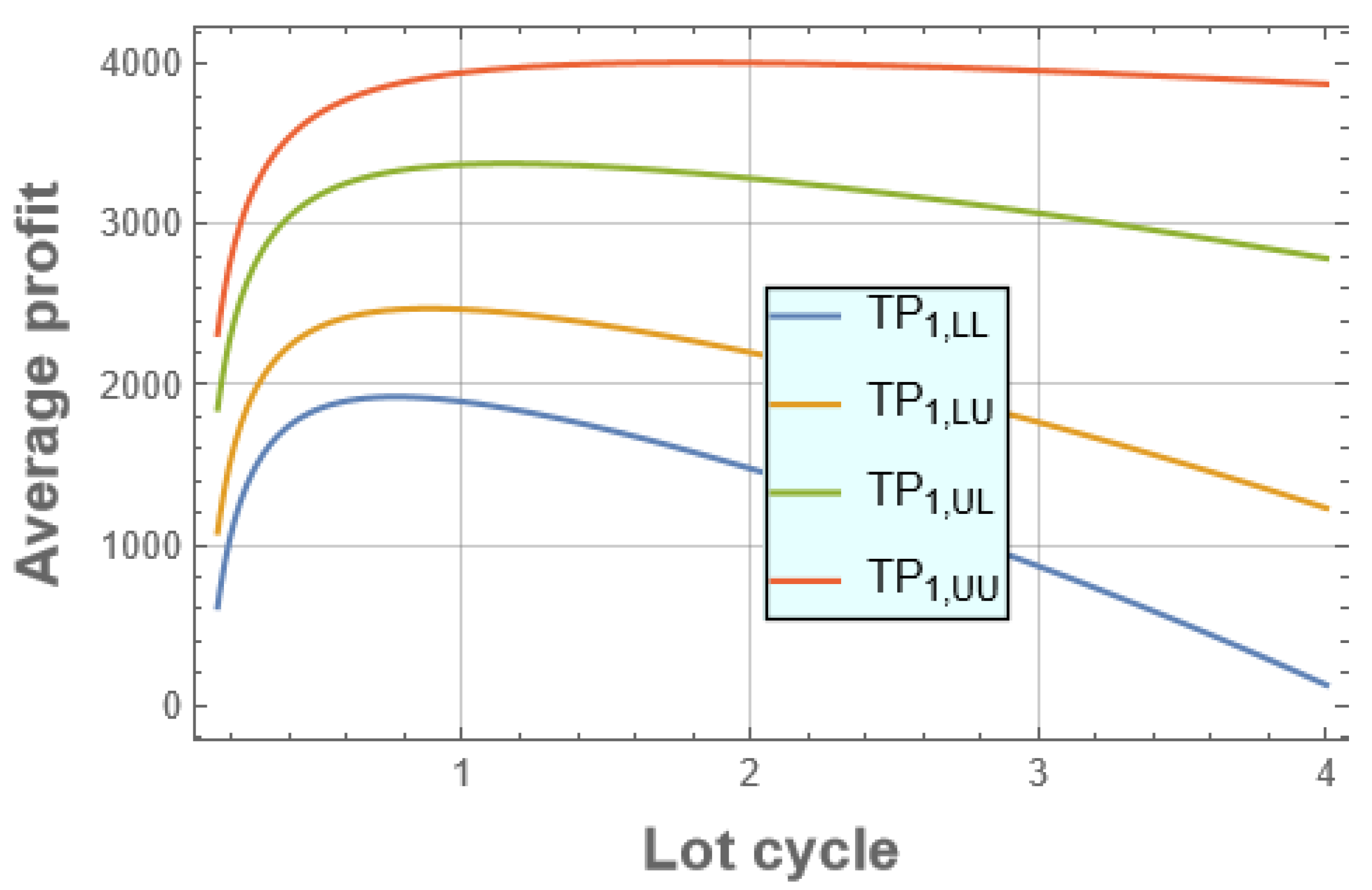For the optimal values of the objective function, the total average profit is ${\widetilde{T{P}_2}}^{\mathrm{*}}=\left[\left[\mathrm{1578.07,2271.07}\right],\left[\mathrm{3319.43,4008.27}\right]\right]$ with optimal lot size ${\widetilde{Q_2}}^{\mathrm{*}}=[\left[646.986,649.412\right],[\mathrm{654.310,656.782}]]$ and optimal lot cycle $T^{\mathrm{*}}=1.806$. Figure 2 represents the graph for the total average profit concerning the time cycle.

Case 2.

When $\widetilde{I_2}(t)$ is generalized Hukuhara differentiable of the second type

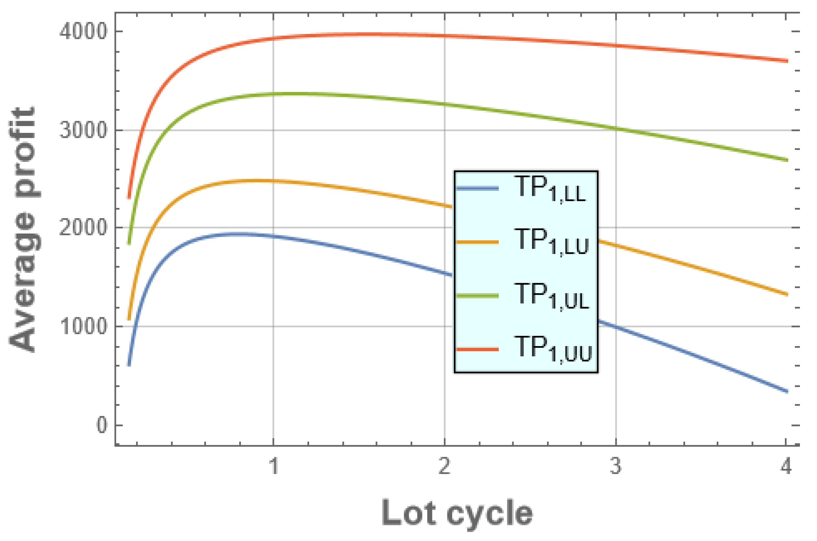
Then, the values of intermediate parameters as follows: ${\alpha }_1=-298.5$, ${\alpha }_4=-298.1$, ${\alpha }_2=-298.4$, ${\alpha }_3=-298.2$, ${\lambda }_3=1.202, {\lambda }_4=-1.202$, $C_1=-3218.663334803273$, $C_2=632.8537170263784$, $D_1=0.20409$, $D_2=0.09591$, ${\mu }_3=1.095, {\mu }_4=-1.095$, $C_3=-3052.2490842490843$, $C_4=299.7165354330709$, $D_3=0.20475$, $D_4=0.09525$. For the optimal values of the objective function, the total average profit is ${\widetilde{T{P}_2}}^{\mathrm{*}}=\left[\left[\mathrm{1740.72,2372.01}\right],\left[\mathrm{3334.59,3970.55}\right]\right]$ with optimal lot size ${\widetilde{Q_2}}^{\mathrm{*}}=[\left[549.922,547.967\right],[\mathrm{544.104,542.148}]]$ and optimal lot cycle $T^{\mathrm{*}}=1.554$. Figure 3 represents the graph for the total average profit concerning the time cycle.

5.3. Applicability of the Proposed Model

Price has a ripple effect on customers’ appetite for merchandise in the context of retailing. The buying and selling phenomenon in developing or underdeveloped nations almost immediately shows that lower prices lure purchasers to the goods. Price, then, has an impact on average profit as well. However, accurate pricing for an effective strategy design favoring the retailer’s perspective possesses some sense of vagueness. The dilemma in optimal pricing can be adjusted by considering interval decision phenomena in which price can be considered as an interval number having upper and lower bounds of values. However, it is not necessarily true for a real-world business scenario that the values can fit within two specific bounds. Instead, it may be viewed in the type-2 interval number theory, which provides a broader sense of interval uncertainty. Also, showrooms have impacts on the demand regulation. The collection of active stock in the showroom creates additional demand. In the same logic, various associated costs and the stock level can be taken into account in the type-2 interval number setting. Since the impact of pricing on the demand and profit control decisions is very significant and uncertainties arise in designing real-world strategies, the discussed theory and results can be applied in a showroom concerning retail dealing phenomena.

6. Conclusions

Type-2 interval number theory broadens the theory of interval numbers, making the ends of an interval flexible within bounds. The arithmetic characteristics of type-2 interval numbers and their usage for optimizing mathematical models, particularly inventory models, have received focus. It is recommended to use the generalized Hukuhara differentiability technique for discussing differential equation-based mathematical models with type-2 interval uncertainty. Before discussing the solution approach, the solution’s existence and its uniqueness, if it exists, must be verified. This paper contributes to the existence and uniqueness theory for solving type-2 interval-valued differential equations. Also, the solution approach of the type-2 interval-valued differential equations has been discussed in this paper. The utility of the proposed theory has been exercised on an EOQ model. The EOQ model of deteriorated items has been discussed for both cases of generalized Hukuhara differentiability. The main aim of this paper is to establish the theory of solvability of the type-2 interval-valued differential equations. The inventory model is not a priority in this paper. This research is a precursor to differential equation concepts and their utilization in a type-2 interval setting. The current form leaves room for additional investigation in the following areas:

• The theory of integral equations for type-2 interval-valued functions may be introduced following the footsteps of this paper.
• More implicit and explicit characteristics of type-2 interval-valued calculus may have emerged as an epicenter for future research.
• This theory’s fractional order counterpart may be a fruitful consequence of the proposed approach.
• We have discussed a popular lot-size model as an application of the proposed theory. We have shortened our analysis because the inventory model was not our main concern. In the future, a robust approach to model formulation and optimization associated with raw data from the market will be the ultimate consequence of the proposed theory.