A New Measure for Determining the Equivalent Symmetry of Decomposed Subsystems from Large Complex Cyber–Physical Systems

Abstract

In this paper, we propose a new consistency measurement for classification rule sets that is based on the similarity of their classification abilities. The similarity of the classification abilities of the two rule sets is evaluated though the similarity of the corresponding partitions of the feature space using the different rule sets. The proposed consistency measure can be used to measure the equivalent symmetry of subsystems decomposed from a large, complex cyber–physical system (CPS). It can be used to verify whether the same knowledge is obtained by the sensing data in the different subsystems. In the experiments, five decision tree algorithms and eighteen datasets from the UCI machine learning repository are employed to extract the classification rules, and the consistency between the corresponding rule sets is investigated. The classification rule sets extracted from the use of the C4.5 algorithm on the electrical grid stability dataset have a consistency of 0.88, which implies that the different subsystems contain almost equivalent knowledge about the network stability.

1. Introduction

A cyber–physical system [1,2,3] combines environmental awareness, embedded computing, and network communications to form a multi-dimensional heterogeneous complex system that integrates real-time sensing, dynamic control, and information services. The large, complex CPS can be decomposed into subsystems with inherent symmetry or equivalent symmetry to simplify the control synthesis and reduce the computational burden. Intelligent decision-making is one of the important methods used by CPSs to process sensing data. A neural network has been incorporated into the fuzzy controller to provide the learning capability, and an adaptive neural fuzzy inference system (ANFIS) has been designed to deal with the dynamic data of a cyber–physical system [4]. A fuzzy-algorithm-based cyber–physical system has been proposed for use in supply chain management with a fault detection technique [5]. A deep learning classification sound system has been proposed for execution in a cyber–physical system [6]. Deep-learning-based methods of attack detection for cyber–physical systems’ cybersecurity are summarized in [7].

A rule-based classification system is a useful tool for dealing with the classification problems in CPSs. Various classification rule-mining algorithms (CRMAs) have been proposed for organizing and formulating the discovery of important relationships hidden in the data. Some of them have achieved a very high predication accuracy or have obtained compact rule bases [8,9,10,11,12,13,14,15], while others have pursued a tradeoff between accuracy and interpretation [16,17,18,19]. The choice of the CRMA for a specific problem in a CPS is a strategic decision which often has to be made early in the classification process for sensing data. This choice will significantly affect the success of the entire classification project, making it absolutely vital that an appropriate technique be chosen [20]. The evaluation of the predictive performance on a set of testing samples is taken as the criterion to choose which of these CRMAs should be preferred for a specific problem. The CRMA is usually evaluated based on its accuracy on the testing samples and the number of classification rules obtained. A great number of classification rule sets with quite different prediction results and interpretations may be discovered using various algorithms and different settings.

In this paper, we focus on the consistency of the classification rule sets extracted from the data in the subsystems of a complex CPS in order to evaluate whether the same knowledge is discovered or not. We assumed that the large cyber–physical system is decomposed into multiple subsystems. The consistency of the knowledge contained in the different subsystems used for decision-making was taken as a measurement of the similarity between the different subsystems. A new measure of the consistency between two classification rule sets is proposed. The proposed consistency measurement can be used as a criterion with which to select classifiers. When different classification models are compared, the prediction accuracy is often considered more important than the other criteria in the existing literature, such as in [11,13,14], etc. Our experiments showed that a classifier with a high average consistency measure value for different runs on a dataset can give both a lower standard deviation and a higher average test accuracy. Thus, when there is no significant difference among the accuracies on a dataset, the consistency measure could serve as a criterion for the selection of a better classifier. This paper makes the following two contributions:

(1)

The consistency between two rule sets of different classifiers is defined. This consistency measure can not only measure the consistency of a classifier, but also measure the similarity of two subsystems decomposed from a large complex CPS.

(2)

In order to measure the similarity of a pair of rules from different rule sets, the concept of the core space of a rule was analyzed, and the similarity of a pair of rules was defined on the basis of the intersection of the core spaces.

This paper is organized as follows. In Section 2, the work related to the similarity of classification rule sets is further elaborated. In Section 3, firstly, the method proposed by [21] is analyzed. Secondly, a new consistency measure for the classification rule sets based on the partitions of the feature space is proposed. In Section 4, the evaluation procedures are illustrated with some examples, and the characteristics of the consistency measure are examined. Some practical experiments are also performed on the algorithm with various datasets. The conclusions of this study are included in Section 5.

2. Related Work

The consistency of different rule sets obtained from different subsystems of a CPS that can be used as a measurement for the equivalent symmetry of the decomposed subsystems can be measured (or compared) in different ways. This section discusses several studies that various researchers have carried out on the consistency of different classification rule sets. There are several definitions of the consistency of classification, and most of them try to figure out whether a repeated application of a rule-based classifier on similar training data will produce a similar classification.

The main difference between these different definitions is what they consider to be the result: the accuracy, the predications, or the rule set itself [21]. In [22], the term “classifier consistency” refers to the reliability of the classification. Similar to this definition, the term “classification consistency” in [23] refers to the probability that an examinee will be classified into the same grade under repeated administrations of an assessment. In [24], the authors propose a classification consistency method for use in complex assignment based on the multinomial and compound multinomial models. In [25], the authors introduce new procedures for computation and asymptotic statistical inference for classification consistency and accuracy indices specifically designed for cognitive diagnostic assessments. The new classification indices can be used as important indicators of the reliability and validity of the classification results produced by cognitive diagnostic assessments.

Some techniques consider consistency by comparing the predictions from the rule sets and give a numerical index. For example, in [26], a classifier was consistent if, under different training sessions, rule sets that produced the same classification of the samples were generated. There was a slight difference in the definition provided in [27], which referred to consistency as the ability of an algorithm to extract rules with the same degree of accuracy under different training sessions. These approaches make it rather easy to find numerical values, but the danger lies in that, sometimes, very different rules can in fact produce similar predictions and accuracies.

Johansson [20] believed that an algorithm is consistent if it extracts similar rules (i.e., similar partitions of the feature space) every time when it is applied to a specific dataset. However, it is very hard to find a general measure applicable to partitions with unlimited boundaries on some attributes. To deal with the unlimited boundary issue, the paper [21] focuses on the individual rule and provides a numerical similarity measure which can help to examine the different degree between the two rule sets A and B.

$$\begin{array}{c}\hfill \sigma (A,B)=\frac{1}{2N}\sum _{r\in A,B}{N}_r^{opposite}\end{array}$$

(1)

$$\begin{array}{c}\hfill N_r^{opposite}=\left\{\begin{array}{c}\underset{q\in B}{max}{N}_{r\cap q},r\in A;\hfill \\ \underset{q\in A}{max}{N}_{r\cap q},r\in B;\hfill \end{array}\right.\end{array}$$

where q and r are two rules from rule sets A and B, respectively, and have the same consequence. $N_{r\cap q}$ is the number of samples covered both by rule r and rule q. This measure focuses on the definition: the similarity of the rule sets and the consistency of the two rule sets are derived by a weighted average of similarities between individual rules in both rule sets. The main idea behind this definition is that two rule sets are similar if they use ‘similar’ rules to make classification decisions.

The various definitions of similarity between the different classification rule sets mentioned above are based on classification results or classification rules. They do not consider whether the partitions of the whole feature space are similar. In this paper, a consistency measurement based on the feature space division is proposed; it is an extension of the above definition in some cases.

3. Classifier Consistency

This section starts by conducting some comparative analyses between various consistencies; then, a new consistency measure of the classification rule sets is proposed.

3.1. Comparative Analysis

The consistency of two different classification rule sets indicates the similarity of their classification abilities. The classification ability of a rule set cannot be measured by the classification result or the number of samples covered by the rule set. The similarity of rule sets based on classification results or samples covered by the rule set may fail in situations where each pair of rules for two classifiers is not similar, although their rule sets are similar on the whole, as shown in Figure 1. The amount of similarity between each pair of rules is determined by the number of observations that these rules cover jointly and their label similarly. For a classification problem, the individual rule is not so vital compared with the whole rule set. The paper [21] focuses on the similarity of individual rules. Thus, it may give a lower similarity even though the two rule sets have similar partitions of the feature space. In an example shown in [21], the approach obtains a similarity of 0.80 even if the partitions for each class of the feature space are completely identical. To deal with the unlimited boundary issue, this paper proposes an algorithm (Algorithm 1), using the observations to determine a proper finite boundary for the partition of the feature space.

Algorithm 1: Determine the core space of rule r.

3.2. Comparative Analysis

In what follows, the differences between the aforementioned definitions are compared and analyzed in Figure 1. Assume an algorithm has provided two rule sets $A=\left\{r_i\right|i=1,2,\cdots ,7\}$ and $B=\left\{q_i\right|i=1,2,\cdots ,7\}$ to divide the Dot from the Star observations and the rules in each rule set are mutually exclusive and exhaustive. For this example, it is assumed that all rules, except for $r_5,r_6,r_7$, and $q_5,q_6,q_7$, predict the class that will be Dot. We can observe from Figure 1 that A and B create very similar (but not the same; the difference is shown by the colored part) decision boundaries between the two classes and that they make exactly the same predictions for all observations. This means that these two rule sets are completely consistent according to the definitions provided in [26,27], as they provide the same predictions and therefore the same level of accuracy. If a new sample, which lies in the colored part, is introduced, the predictions mad by these two rule sets would be different. Hence, the classification abilities of A and B are slightly different because of their different partitions of the feature space. Therefore, the consistency measure value should not be 1. The definitions in [26,27] should be improved for measuring the consistency of the two rule sets.

Let us look at the conclusion for Figure 1 drawn from the definition in [21]. The similarity of the two rule sets shown in Figure 1 can be calculated with (1) as 0.78. The figure shows that the classification abilities (or the rule sets of each class) of A and B are very similar. Therefore, 0.78 is lower than the estimatefor evaluating the similarity. The reason for this is that the paper [21] focused on the similarity of individual rules, and ignored the similarity of the whole rule sets. The consistency value given by the proposed consistency measurement in Algorithm 2 is 0.98, which is in agreement with the estimate.

Algorithm 2: The Consistency Measure Algorithm (CMA).

1  Step 1: For each rule $r\in A_c,q\in B_c$, where $A_c$ and $B_c$ are two different rule sets of class c, respectively, find the core spaces, $H\left(r\right)$ and $H\left(q\right)$, using the algorithm shown in Algorithm 1. Then, compute the corresponding volumes: $V\left(H\right(r\left)\right)$ and $V\left(H\right(q\left)\right)$. The volume of rule sets $A_c$ and $B_c$ of class c denoted by $V_{A_c}$ and $V_{B_c}$ can be calculated as follows:

2              $V_{A_c}=\sum _{r\in A_c}V\left(H\left(r\right)\right),V_{B_c}=\sum _{q\in B_c}V\left(H\left(q\right)\right)$

3  Step 2: For each rule $r\in A_c$ and for each rule $q\in B_c$, compute the volume of the intersection of the two core spaces, which is denoted as $V\left(H\right(r)\cap H(q\left)\right)$. Then, the volume of the intersection of the two rule sets $A_c$ and $B_c$ of class c can be computed as:

4              $V(A_c,B_c)={\sum }_{r\in A_c}{\sum }_{q\in B_c}V(H\left(r\right)\cap H\left(q\right))$

5  Step 3: The similarity measure between the two rule sets $A_c$ and $B_c$ of class c is defined as:

6              $Sim(A_c,B_c)=\frac{2V(A_c,B_c)}{V_{A_c}+V_{B_c}}$

7  Step 4: The consistency measure between the rule sets A and B, which can be considered as a weighted average of the similarities between classes in both rule sets, is defined as:

8       $Con(A,B)=\frac{1}{2}{\sum }_c{\omega }_{A_c}Sim(A_c,B_c)+\frac{1}{2}{\sum }_c{\omega }_{B_c}Sim(B_c,A_c)$

9  The weight factors can be chosen as the proportion of the observations covered by $A_c$ and $B_c$, respectively,

10              ${\omega }_{A_c}=\frac{N_{A_c}}{N};{\omega }_{B_c}=\frac{N_{B_c}}{N},$

11  where $N_{A_c}$, $N_{B_c}$ are numbers of the observations covered by the rule sets $A_c$ and $B_c$, respectively. N is the numbers of the observations in the dataset X.

Figure 2 shows the variants, $A^{\prime }=\left\{r_i^{\prime }\right|i=1,2,\cdots ,7\}$ and $B^{\prime }=\left\{q_i^{\prime }\right|i=1,2,\cdots ,7\}$, of rule set A and rule set B. We can see that Figure 1 and Figure 2 have consistent decision boundaries, but compared with rule set A and B, the individual rules in the new rule sets show some changes. The consistencies given by the definitions in [26,27] do not change, since the decision boundaries of $A^{\prime }$ and $B^{\prime }$ are same as those of A and B. The consistency given by the definition in [21] greatly changed from 0.78 (between A and B) to 0.97 (between $A^{\prime }$ and $B^{\prime }$) due to the changes in the individual rules in the new rule sets. This implies that the similarities between individual rules may lead to very different results being obtained for the consistency between a pair of rule sets. The consistency between the new rule sets $A^{\prime }$ and $B^{\prime }$ given by the proposed measurement is 0.98.

3.3. Core Space of a Rule

When considering the similarity of a pair of classification rules obtained from two different rule sets, whether the classification capacities are similar or not is considered. We usually care about whether the two rules assign the same class labels for both the observations and the unseen samples.

A rule can determine a region in the feature space by its antecedent and assign the samples that fall in this region the same class label using its consequence. We denote the region determined by rule r as $H^r$. $H^r$ is composed of two different parts. The first one is the hyper-cuboid region in the feature space decided by the observations covered by rule r and denoted as $H_r$. Naturally, the other one is $H^r\backslash H_r$. $H^r\backslash H_r$ is called the generalizing region of rule r. For rule r, the region $H_r$ is more important than the generalizing region $H^r\backslash H_r$ for the following two reasons. First, we have more confidence in the classification results of the samples located in the region $H_r$ than those falling in $H^r\backslash H_r$, because there are no observations in the region $H^r\backslash H_r$ and the rule r could not provide enough information about the classification results over this region. Secondly, the boundaries of the generalizing region are mainly decided by the algorithm, while the boundaries of the region $H_r$ depend on both the observations and the algorithm. The boundaries of the generalizing region are variable according to different algorithms. Two similar rules obtained from different algorithms may have very different generalizing regions even if they covered the same observations.

Some regions determined by the rules and the observations covered by the rules are shown in Figure 3. Figure 3a shows the rule set obtained using C4.5 [9] over a one-dimensional synthetic dataset and the regions determined by the rules and the observations covered by each rule. The rule set is:

$r_1$: IF $x\in (-\infty ,4.96]$, THEN Class is Star;

$r_2$: IF $x\in (4.96,6.97]$, THEN Class is Dot;

$r_3$: IF $x\in (6.97+\infty )$, THEN Class is Star.

Figure 3b shows the rule set obtained by CART [15] over the same one-dimensional synthetic dataset and the regions determined by the rules and the observations covered by each rule. The rule set is:

$q_1$: IF $x\in (-\infty ,5.56]$, THEN Class is Star;

$q_2$: IF $x\in (5.56,7.25]$, THEN Class is Dot;

$q_3$: IF $x\in (7.35+\infty )$, THEN Class is Star.

The C4.5 algorithm and the CART algorithm create different partitions of the one-dimensional feature space; see $H^{r_i}$ and $H^{q_i}$ ($i=1,2,3$) in Figure 3. When considering the consistency between the two rule sets, while they might seem slightly different at first, closer inspection will reveal that the regions $H_{r_i}$ and $H_{q_i}$ took up by the observations determined by the rule $r_i$ and $q_i$ ($i=1,2,3$) are exactly same. In other words, the two rule sets create different decision boundaries—i.e., the boundaries of $H^{r_i}$ and $H^{q_i}$. Thus, $H^{r_i}$ is different from $H^{q_i}$ ($i=1,2,3$). The reason for this is the difference in the generalizing regions of each rule, which is caused by the different methods used by the C4.5 algorithm and the CART algorithm for the partition of the margins. The two rule sets seem to have an identical classification ability when considering the regions $H_{r_i}$ and $H_{q_i}$$(i=1,2,3)$. When considering the uncertainty of generalizing regions, the similarity between two rules $r_i$ and $q_i$ ($i=1,2,3$) derived from the comparison of $H_{r_i}$ and $H_{q_i}$ may be more reasonable. However, this may fail in situations where the regions $H^r$ and $H^q$ of a pair of rules r and q suffer from the unlimited boundary problem.

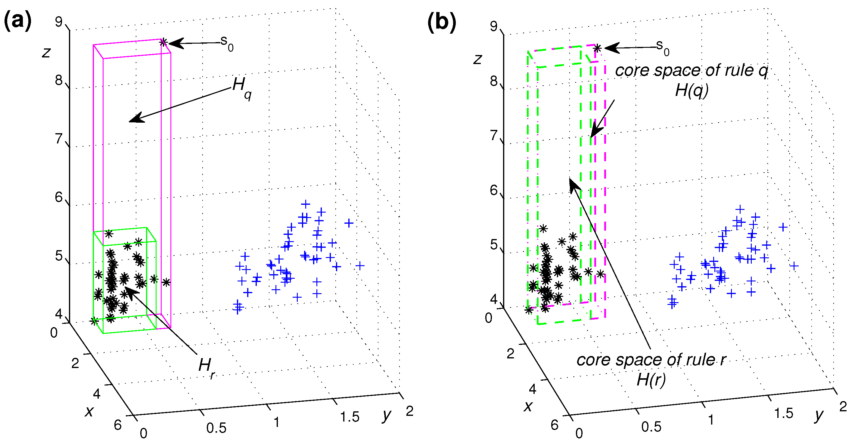
Figure 4a shows two rules r: IF $x\in [0,1.9]$ and $y\in [0,0.5]$, THEN Class is *; q: IF $x\in [0,1.9]$ and $y\in [0,0.6]$, THEN Class is *. The rules r and q come from two different rule sets over a three-dimensional synthetic dataset and are very similar. However, neither have any conditions for the third feature z. The regions $H_r$ and $H_q$ are not similar as the rules show, since the observation $s_0$ is not covered by rule r. To deal with unlimited boundary issue, the regions $H_r$ and $H_q$ should be tuned to a uniform finite bound for the unconditional features (e.g, feature z) in order to fairly evaluate the similarity of the two rules. We propose Algorithm 1 to redetermine proper boundaries of the region $H_r$ determined by the observations covered by rule r. The tuned region is called the core space of the rule r, denoted as $H\left(r\right)$. The core space of a rule can not only describe the classification ability of the rule well, but can also deal with the unlimited boundary problem. As shown in Figure 4b, the core spaces of the two rules r and q are similar.

If two rules from different rule sets cover the same observations, essentially, they are very similar because the core spaces of the two rules are same. The intersection of the core spaces can indicate the similarity of classification abilities of two rules. The similarity between the two rules is evaluated by comparing the core spaces of the rules.

3.4. The New Consistency Measure

When considering the consistency of the classification rule sets, whether their classification ability is similar or not is crucial. Hence, we consider the rules for one class as a rule set of the class and measure the similarity of two rule sets for this class. Firstly, the similarity of the two rule sets of a class is defined by comparing the core spaces of the rules in the two rule sets of this class. Then, the consistency between the two rule sets of classifiers is defined as the weighted average of the similarities between the rule sets of each class. The main idea behind our proposed consistency measure is that two rule sets of classifiers are consistent if their partitions of the feature space are similar. The consistency not only considers the similarity of the assignment of class labels of two rule sets but also the similarity of the partitions of the feature space. i.e., they predict the samples under similar probability distributions.

When the regions covered by two rules contain infinite boundaries, it is difficult to calculate the similarity of the two rule directly and simply. Algorithm 1 constrains the infinite boundary to the region covered by the observations, which is conducive to the simplicity of the comparison for similarity of a pair of rules. In fact, partition of the feature space by a rule set represents its classification ability. The similarity of a pair of rules based on the similarity of their core spaces is defined. The reason is which core space of rule covered by observations is more reliable for classification.

The similarity of a pair of rule sets (or a pair of rules) is considered as the similarity of their classification abilities—that is, the partition of the whole feature space by the rule set. When the rule contains an infinite boundary, it is difficult to make the comparison of a pair of rule sets (or pair of rules). We limit the infinite region covered by the rules within the scope covered by the observations. The core space of a rule is the limit of the region covered by the rule on the coverage area of the observations. We analyze the similarity of a pair of rules by comparing their core spaces. The reason for this is that the classification algorithms tend to partition the region covered by the observations, and the classification boundary usually lies in the margin of different classes, while we tend not to care much about the region far away from the observation points.

Given two rule sets A and B and a dataset X of the observations, it can be seen that the rules in each rule set are mutually exclusive and exhaustive. $A_c\subseteq A$ and $B_c\subseteq B$ are the rule sets of class c, respectively. For each rule $r\in A\cup B$, the core space $H\left(r\right)$ can be determined using the algorithm shown in Algorithm 1. $V\left(H\right(r\left)\right)$ represents the volume of $H\left(r\right)$. The proposed consistency measure algorithm is as follows:

It is easy to prove that the proposed consistency measure satisfied the following properties. For two rule sets $R_1$ and $R_2$, we have:

• Symmetric: $Con(R_1,R_2)=Con(R_2,R_1)$;
• Non-negativity: $Con(R_1,R_2)\ge 0$;
• If the two rule sets $R_1$ and $R_2$ are exactly the same, then the consistency should be maximal—i.e., $Con(R_1,R_2)=1$;
• If the two rule sets $R_1$ and $R_2$ provide different classifications for each input observation, then the consistency should be minimal—i.e., $Con(R_1,R_2)=0$;

For the similarity of (1), $\sigma (A,B)=1$ if and only if for all $r\in A$, there exists a rule $q\in B$, such that r and q cover the same samples and assign the same class labels to the samples. Therefore, the number of rules in rule set A is equal to that of rule set B. Meanwhile, the proposed similarity has less request, which focuses more on the similarity of the partitions of the feature space by the rule sets for each class. Furthermore, let $Assignment\left(A\right)$ denote the assignments of the samples in the dataset X by rule set A, and $Accuracy\left(A\right)$ denote the accuracy of rule set A for the dataset X. We have the following proposition about the relation of the four mentioned kinds of consistency measures.

Proposition 1.

Let A and B be two rule sets which contains mutually exclusive rules on dataset X. $\sigma (A,B)$ denotes the similarity between A and B using the definition shown in Equation (1), and $Con(A,B)$ denotes the consistency between A and B defined in Algorithm 2. We have

$$\begin{array}{ccc}\hfill \sigma (A,B)=1& \Rightarrow & Con(A,B)=1\hfill \\ \hfill Con(A,B)=1& \Rightarrow & Assignment\left(A\right)=Assignment\left(B\right)\hfill \\ \hfill Assignment\left(A\right)=Assignment\left(B\right)& \Rightarrow & Accuracy\left(A\right)=Accuracy\left(B\right)\hfill \end{array}$$

Proof. 

(1) $\sigma (A,B)=1\Rightarrow Con(A,B)=1$:

$$\begin{array}{ccc}\hfill \sigma (A,B)=\frac{1}{2N}\sum _{r\in A,B}{N}_r^{opposite}=1& \Rightarrow & \sum _{r\in A,B}{N}_r^{opposite}=2N\hfill \\ & \Rightarrow & \forall r\in A,B,N_r^{opposite}=N_r\hfill \end{array}$$

where $N_r$ is the number of samples covered by r. This implies that $\forall r\in A$, there is a rule $q\in B$, where r and q cover the same samples and give the same class label to the samples. Thus, we find that $H\left(r\right)=H\left(q\right),V\left(H\right(r)\cap H(q\left)\right)=V\left(H\right(r\left)\right)=V\left(H\right(q\left)\right)$. Because it is assumed that each rule set contains mutually exclusive rules, $\forall q^{\prime }\in B,q^{\prime }\ne q,V(H\left(r\right)\cap H\left(q^{\prime }\right))=0$, we have $\forall c$,

$$\begin{array}{ccc}\hfill Sim(A_c,B_c)& =& \frac{2V(A_c,B_c)}{V_{A_c}+V_{B_c}}\hfill \\ & =& \frac{2{\sum }_{r\in A_c}{\sum }_{q\in B_c}V(H\left(r\right)\cap H\left(q\right))}{{\displaystyle \sum _{r\in A_c}}V\left(H\left(r\right)\right)+{\displaystyle \sum _{r\in B_c}}V\left(H\left(r\right)\right)}\hfill \\ & =& \frac{2{\sum }_{r\in A_c}V\left(H\left(r\right)\right)}{2V_{A_c}}=1\hfill \\ \hfill Con(A,B)& =& \frac{1}{2}\sum _c{\omega }_{A_c}Sim(A_c,B_c)+\frac{1}{2}\sum _c{\omega }_{B_c}Sim(B_c,A_c)\hfill \\ & =& \frac{1}{2}\sum _c{\omega }_{A_c}+\frac{1}{2}\sum _c{\omega }_{B_c}=1\hfill \end{array}$$

(2) $Con(A,B)=1\Rightarrow Assignment\left(A\right)=Assignment\left(B\right)$:

$Con(A,B)=1$ implies $\forall c,A_c$ and $B_c$ have the same partition of the feature space, so $Assignment\left(A\right)=Assignment\left(B\right)$.

(3) $Assignment\left(A\right)=Assignment\left(B\right)\Rightarrow Accuracy\left(A\right)=Accuracy\left(B\right)$:

Straightforward. □

It is easy to apply the proposed consistency algorithm to the rule sets visualized in Figure 1. Furthermore, as shown in the next section, the proposed consistency algorithm can be applicable to the rule sets altered from other representation forms, such as decision trees and decision tables. Since the rule extraction algorithms, such as the algorithm shown in [14], are able to extract mutually exclusive rules from different types of black box models, the proposed measure of consistency can also help to test whether the extracted rule sets are similar to other rule sets or the black box models are consistent with the existing knowledge.

4. Empirical Studies

In this section, we perform several experiments with some benchmark datasets from the Machine Learning repository [28]. The data can be regarded as the sensing data from the sensors of the CPS. The description of the pertinent datasets is covered in

Table 1. Description of datasets from the UCI repository used in the experiments.

No.	Data Set	Size	Attributes	Class
1	Blocks	5473	10	5
2	Breast-W	699	9	2
3	Image	2310	19	7
4	Iris	150	4	3
5	Magic	19,020	10	2
6	Mammographic	961	5	2
7	Parkinson’s	195	22	2
8	Pima	768	8	2
9	Transfusion	748	4	2
10	Vehicle	846	18	4
11	Vertebral-2C	310	6	2
12	Vertebral-3C	310	6	3
13	Wall-2A	5456	2	4
14	Wall-4A	5456	4	4
15	Wall-24A	5456	24	4
16	Waveform	5000	40	3
17	Wine	178	13	3
18	EGS	10,000	12	2

. Five decision tree algorithms—C4.5, CART, J48graft [29], RandomTree [30], and REPTree—are used in the experiments for extracting the rules. The decision trees returned by the algorithms can be easily converted into a set of mutually exclusive rules via creating a rule for each path from root to leaf node of the trees. All the classifiers are implemented by using the Weka machine learning toolkit [31].

4.1. Demonstration on Electrical Grid Network Data Set

The first experiment is a demonstration on the electrical grid network dataset. We show the evaluation of the equivalent symmetry between different subsystems of the electrical grid network using the proposed consistency measurement shown in Algorithm 2.

The electrical grid stability dataset is used for the local stability analysis of the 4-node star system (electricity producer is in the center), implementing the decentral smart grid control concept. It contains 10,000 samples and is stratified and divided into tenfold of (approximately) equal size. Each time, one fold, which could be regarded as a set of data points from the subsystem decomposed from the original power grid networks, is left out of the whole dataset to train a C4.5 decision tree. As a result, there are ten C4.5 classification rule sets based on the “Electrical Grid Stability (EGS) Data Set”.

Then, the proposed consistency measurement can be used to evaluate the similarity between the different C4.5 classification rule sets. For each of the ten tree classifiers, we show their consistency with the other trees pairwise. The results of the C4.5 algorithm are shown in

Table 2. The consistencies between different subsystems of the electrical grid network.

Subsystem	2	3	4	5	6	7	8	9	10
1	0.93	0.83	0.92	0.90	0.90	0.92	0.91	0.91	0.91
2		0.82	0.90	0.89	0.90	0.91	0.92	0.90	0.90
3			0.82	0.80	0.81	0.82	0.75	0.73	0.82
4				0.89	0.89	0.90	0.91	0.90	0.90
5					0.90	0.90	0.91	0.89	0.91
6						0.89	0.90	0.89	0.88
7							0.90	0.93	0.93
8								0.90	0.90
9									0.92

. As can be seen from Table 2, the average consistency is 0.88 and except for subsystem 3, the consistencies between the other subsystems are almost $0.90$, indicating that the knowledge about the electrical grid stability contained in each subsystem is almost same. However, subsystem 3 is slightly different from the other subsystems in that it has different knowledge about the electrical grid stability.

4.2. Comparison of Rule Sets Obtained by Different Algorithms

This experiment is performed on the widely used Iris dataset and Wavefrom dataset. We train various decision tree learners—namely, C4.5, CART, J48graft, RandomTree, and REPTree—on the two datasets. On both of the two datasets, the five decision trees provide different rule sets. For example, on the Iris dataset, the number of rules in the rule set from C4.5 is 5, but that from J48graft is 11. On the larger dataset (Wavefrom), the number of rules increases rapidly (C4.5: 330; CART: 78; J48graft: 767; RandomTree: 668; and REPTree: 102). It is difficult to assess whether the extracted knowledge is the same for these algorithms due to the large and complex rule sets involved. While an explicit conversion is often possible, the proposed consistency measure is used to test the consistency between each pair of the obtained rule sets. The results gained on Iris data set are shown in

Table 3. Consistencies on the (a): Iris dataset and (b) the Waveform dataset.

(a)
Between algorithms	C4.5	CART	J48graft	RandomTree	REPTree
C4.5	1.00	1.00	0.99	0.86	0.92
CART		1.00	0.99	0.87	0.92
J48graft			1.00	0.84	0.92
RandomTree				1.00	0.87
REPTree					1.00
(b)
Between algorithms	C4.5	CART	J48graft	RandomTree	REPTree
C4.5	1.00	0.54	0.98	0.48	0.58
CART		1.00	0.54	0.47	0.65
J48graft			1.00	0.48	0.58
RandomTree				1.00	0.49
REPTree					1.00

a. The rather high scores indicate that most of the extracted rule sets are very similar and contain similar knowledge. Table 3b shows the results gained on the Wavefrom dataset. The low scores (except for the score between C4.5 and J48graft) indicate that the extracted rule sets are not similar and contain quite different knowledge.

4.3. Consistency of C4.5 and the Other Decision Tree Algorithms

In this experiment, the similarities of the C4.5 algorithm and the other algorithms (CART, J48graft, RandomTree, and REPTree) are studied based on the consistency of the rule sets they returned on the seventeen benchmark datasets described in Table 1. The C4.5 decision tree is used as a criterion for comparison due to the fact that the C4.5 decision tree is the most commonly used classical algorithm. The consistency measure values on the seventeen datasets between the rule sets from C4.5 and those from the other algorithms are shown in

Table 4. Consistencies between C4.5 and other algorithms.

Data Set	CART	J48graft	RandomTree	REPTree
Blocks	0.67	0.97	0.08	0.53
Breast-W	0.65	1.00	0.45	0.49
Image	0.75	0.98	0.50	0.61
Iris	1.00	0.99	0.86	0.92
Magic	0.55	0.92	0.37	0.47
Mammographic	0.75	1.00	0.47	0.76
Parkinson’s	0.74	0.92	0.70	0.81
Pima	0.96	1.00	0.51	0.87
Transfusion	0.98	0.99	0.81	0.93
Vehicle	0.71	0.83	0.33	0.53
Vertebral-2C	0.95	0.99	0.93	0.92
Vertebral-3C	0.92	0.99	0.84	0.87
Wall-2A	1.00	1.00	0.99	0.99
Wall-4A	1.00	1.00	0.99	0.99
wall-24A	0.98	0.98	0.49	0.97
Waveform	0.54	0.98	0.48	0.58
Wine	0.76	0.97	0.84	0.79
Mean	0.82	0.97	0.63	0.77

.

It can be seen that the average consistency value obtained between C4.5 and J48graft on the seventeen datasets is 0.97, which indicates that the rule sets obtained by the two algorithms divided the feature space into very similar regions for all seventeen datasets. This is not surprising when considering that the latter is an improvement of the former.

The mean consistency values between C4.5 and CART are bigger than those between C4.5 and RandomTree and between C4.5 and REPTree, which shows that C4.5 and CART can provide similar rule sets in most of situations. In other words, the rule sets obtained by C4.5 and CART often divide the feature space into similar regions. The paired Student’s t-test is employed to justify if an algorithm is statistically more similar to C4.5 than another on the seventeen datasets. The result shows that compared with C4.5, the consistency differences between the algorithms (CART, RandomTree, and REPTree) are significant, and compared with RandomTree and REPTree, CART is more similar to C4.5.

The consistency values of the rule sets obtained by C4.5 and RandomTree are small for most of the cases. The rule sets returned by the RandomTree algorithm often have many more rules than those returned by the C4.5 algorithm. The reason for this is that the RandomTree algorithm pursues the nicety partitions of the feature space, which can help the training accuracy to reach as high as 100% for a lot of problems. This kind of overfitting leads to a huge number of rules which would divide the sample space into too many small regions. Therefore, the RandomTree algorithm can hardly carry out the similar partition of the feature space with other algorithms.

From Table 4, it can be concluded that in general the data sets which lead to simpler rule sets may be able to achieve higher consistency values between the algorithms. For instance, the Iris dataset with a small number of instances (150) and wall-2A with only two attributes and a more concentrated sample distribution are easy to separate. Therefore, the rule sets returned by the algorithms consist of a few very compact rules. In the Iris dataset and the Wall-2A dataset, only two attributes are used for classification by all the algorithms. Using the rule sets from the C4.5 algorithm and the other algorithms on the two rule sets, high scores have been achieved; see Table 4. In contrast, the datasets which led to a great number of complex rules struggle to obtain higher consistency values between the algorithms. An example of this is the Waveform dataset, which has 5000 instances and 40 attributes. On the Waveform dataset, the number of rules obtained from the algorithms of C4.5, CART, J48graft, RandomTree, and REPTree are 330, 78, 767, 668, and 102, respectively. It can be found in Table 4 that the consistency values obtained on the Waveform dataset are much smaller than those obtained on the other data sets.

4.4. Selection of Algorithm by the Proposed Consistency

In this experiment, we aim at the relation between the proposed consistency measure and the accuracy evaluation criterion. Six datasets are used in this experiment. They are Iris dataset, Pima dataset, Transfusion dataset, Vehicle dataset, Wavefrom dataset and Wine dataset.

In each dataset X, the samples are divided into two parts, $X_1$ and $X_2$ sized as $50\%$-$50\%$ of the total samples. $X_1$ is used for training and testing. $X_2$ is treated as the observation for the consistency evaluation. In $X_1$, we randomly draw $20\%$ samples for testing, and the remaining samples are used for training a decision tree classifier. Furthermore, the experiments are repeated ten times by randomly generating an 80-20 split of $X_1$. The experiments are performed with the algorithms C4.5, CART, J48graft, RandomTree, and REPTree.

For each algorithm, the average test accuracy of the ten classifiers, the standard deviation, and the average consistency of the 45 ($C_{10}^2$) pairs are shown in Figure 5. The figure shows that, in general, the higher the consistency is, the lower the standard deviation will be, while the higher the consistency is, the higher the accuracy will be. This implies that not only is consistency coherent with the accuracy and standard deviation, but that the consistency can be use to characterize the general stability in probability. For a situation where the prediction accuracy on a dataset obtained using different algorithms is not significant, the one with a higher consistency score could be the better classifier for the dataset.

For instance, we compare the C4.5 and CART on the Pima data set. The average accuracy of C4.5 over the ten runs is 73.77%, with a standard deviation of 0.0438, and that of CART is 74.81% with a standard deviation of 0.0420. The difference in the average accuracies given by C4.5 and CART is not significant. The proposed consistency measure can be used to find the similarity between the different runs for each algorithm. For each of the ten tree classifiers, we show their consistency with the other trees measured on $X_2$. The results of C4.5 are shown in

Table 5. The consistencies between the ten runs on the Pima dataset (a): C4.5 and (b): CART.

(a) C4.5
Runs	2	3	4	5	6	7	8	9	10
1	0.69	0.76	0.66	0.70	0.56	0.76	0.76	0.68	0.64
2		0.88	0.77	0.77	0.80	0.88	0.88	0.78	0.95
3			0.77	0.82	0.67	1.00	1.00	0.82	0.80
4				0.70	0.66	0.77	0.77	0.69	0.75
5					0.63	0.82	0.82	0.83	0.70
6						0.67	0.67	0.66	0.86
7							1.00	0.82	0.80
8								0.82	0.80
9									0.73
(b) CART
Runs	2	3	4	5	6	7	8	9	10
1	0.99	0.99	0.99	0.81	0.69	0.99	0.87	0.94	0.99
2		1.00	1.00	0.82	0.70	1.00	0.88	0.95	1.00
3			1.00	0.82	0.70	1.00	0.88	0.95	1.00
4				0.82	0.70	1.00	0.88	0.95	1.00
5					0.64	0.82	0.88	0.87	0.82
6						0.70	0.79	0.67	0.70
7							0.88	0.95	1.00
8								0.87	0.88
9									0.95

a, and the average consistency is 0.77. The consistency results of CART are shown in Table 5b, and the average consistency is 0.88. A paired t-test shows that the observed consistency difference is significant. Based on these results, we believe that CART is the better learner for this dataset, as it not only provides a comparable accuracy on this dataset but is also more consistent than the tree classifiers constructed using the C4.5 algorithm.

4.5. Consistency of the C4.5 Decision Tree

In this experiment, we study the consistency of the C4.5 on four real-life datasets. The information of the Wine dataset, the Waveform dataset, and the Pima dataset can be found in Table 1, and the Wine quality dataset [28] contains 6497 instances, which have 12 attributes with 2 classes.

We first divide all the datasets into a 2/3 training set and a 1/3 test set. Subsequently, to test the consistency of the C4.5 algorithm, the following procedure is applied on the part reserved for training. Firstly, we create 500 new datasets by randomly removing a fixed percentage of the training instances from the part reserved for training. Then, the chosen percentages vary between 5% and 90%. On each of these 500 newly created data sets, which could be from the sensor subnetworks, we build a C4.5 decision tree. For each tree, we first measure the accuracy on the test set. An overview of the performance distributions is given in Figure 6 and Figure 7. The percentages in the legend indicate the number of remaining samples in the dataset reserved for training. It is easy to see that the prediction accuracy increases with the increase in the number of training samples.

In the second step, we compare the consistency of all the classifiers with each other. We first select the first tree and then compare pairwise with each of the other 499 classifiers. The consistency measure values are calculated with the proposed algorithm. Then, we select the second classifier and calculate the consistency measure values for the remaining 498 classifiers and so on. The total number of comparisons is therefore equal to $C_{500}^2$, which is 124,750. An overview of the distribution of the consistency measure values is given in Figure 8 and Figure 9.

We can observe that on all these four datasets, the higher peaks shift rightward in the distribution towards higher consistency levels with the increase in the number of training samples, which indicates that the removal of less samples will lead to more similar classifiers. Furthermore, from the comparison of Figure 8 and Figure 9, we can find that on the Wine dataset and the Wine quality dataset, with the removal of 5% of the data, the algorithm will almost always return the same classifier, as the consistency is usually close to 1. However, this phenomenon does not appear on the Waveform dataset and Pima dataset. We conclude that on the Wine dataset and the Wine quality dataset, the C4.5 algorithm is less influenced by the random removal of training observations than in comparison with the Waveform dataset and Pima dataset. The reason for this is that the Wine dataset and the Wine quality dataset can be easily classified by the C4.5 algorithm, while the Waveform dataset and the Pima dataset struggle to be classified by the C4.5 algorithm. Higher accuracies on the Wine dataset and the Wine quality dataset can be found in Figure 6, and lower ones obtained on the Waveform dataset and Pima dataset are shown in Figure 7.

5. Conclusions

In this paper, the concept of consistency is studied and the rule set itself is used to consider the consistency of the classifiers instead of the prediction and accuracy. This paper proposes the use of an algorithm to calculate a numerical value that can be applied to measure the consistency between different rule sets and the equivalent symmetry of decomposed subsystems from the large and complex CPS. Additionally, the differences between different definitions of consistency are analyzed and discussed. The proposed consistency measure focuses on the similarity of the partitions of the feature space by the rule sets. To deal with the unlimited boundary problem of the partitions of the feature space, the similarity is derived from the intersection of the proposed core spaces of the rules in the two rule sets. Several experiments show how the proposed consistency measure can be used to select different models and algorithms. A classifier with a high average consistency measure value for different datasets from different subsystems can give both a lower standard deviation and a higher average test accuracy; furthermore, the equivalent symmetry of decomposed subsystems can also be evaluated. Future work will focus on the decomposition methods used for large and complex CPS based on the consistency between different subsystems. The similarity of the decision information contained in the subsystems could be used as a criterion for the decomposition and could be combined with other decomposition methods to decompose the complex and large CPS into lower subsystems to reduce the level of complexity and the computation required.

References

1. Poltavtseva, M.; Shelupanov, A.; Bragin, D.; Zegzhda, D.; Alexandrova, E. Key concepts of systemological approach to CPS adaptive information security monitoring. Symmetry 2021, 13, 2425. [Google Scholar] [CrossRef]
2. Wang, C.; Lv, Y.; Wang, Q.; Yang, D.; Zhou, G. Service-oriented real-time smart job shop symmetric CPS based on edge computing. Symmetry 2021, 13, 1839. [Google Scholar] [CrossRef]
3. Pivoto, D.G.; de Almeida, L.F.; da Rosa Righi, R.; Rodrigues, J.J.; Lugli, A.B.; Alberti, A.M. Cyber-physical systems architectures for industrial internet of things applications in Industry 4.0: A literature review. J. Manuf. Syst. 2021, 58, 176–192. [Google Scholar] [CrossRef]
4. Padmajothi, V.; Iqbal, J. Adaptive neural fuzzy inference system-based scheduler for cyber–physical system. Soft Comput. 2020, 24, 17309–17318. [Google Scholar] [CrossRef]
5. Wang, L.; Zhang, Y. Linear approximation fuzzy model for fault detection in cyber–physical system for supply chain management. Enterp. Inf. Syst. 2021, 15, 966–983. [Google Scholar] [CrossRef]
6. Monedero, Í.; Barbancho, J.; Márquez, R.; Beltrán, J.F. Cyber-physical system for environmental monitoring based on deep learning. Sensors 2021, 21, 3655. [Google Scholar] [CrossRef]
7. Zhang, J.; Pan, L.; Han, Q.L.; Chen, C.; Wen, S.; Xiang, Y. Deep learning based attack detection for cyber–physical system cybersecurity: A survey. IEEE/CAA J. Autom. Sin. 2021, 9, 377–391. [Google Scholar] [CrossRef]
8. Pach, F.P.; Gyenesei, A.; Abonyi, J. Compact fuzzy association rule-based classifier. Expert Syst. Appl. 2008, 34, 2406–2416. [Google Scholar] [CrossRef]
9. Quinlan, J.R. C4.5: Programs for Machine Learning; Elsevier: Amsterdam, The Netherlands, 2014. [Google Scholar]
10. Aamir, K.M.; Sarfraz, L.; Ramzan, M.; Bilal, M.; Shafi, J.; Attique, M. A fuzzy rule-based system for classification of diabetes. Sensors 2021, 21, 8095. [Google Scholar] [CrossRef]
11. Alcalá-Fdez, J.; Alcala, R.; Herrera, F. A fuzzy association rule-based classification model for high-dimensional problems with genetic rule selection and lateral tuning. IEEE Trans. Fuzzy Syst. 2011, 19, 857–872. [Google Scholar] [CrossRef]
12. Tiago, d.C.A.; Sanz, J.A.; Dimuro, G.P.; Bedregal, B.; Fernández, J.; Bustince, H. N-Dimensional admissibly ordered interval-valued overlap functions and its influence in interval-valued fuzzy-rule-based classification systems. IEEE Trans. Fuzzy Syst. 2021, 30, 1060–1072. [Google Scholar]
13. Sanz, J.A.; Fernández, A.; Bustince, H.; Herrera, F. IVTURS: A linguistic fuzzy rule-based classification system based on a new interval-valued fuzzy reasoning method with tuning and rule selection. IEEE Trans. Fuzzy Syst. 2013, 21, 399–411. [Google Scholar] [CrossRef] [Green Version]
14. Zhu, P.; Hu, Q. Rule extraction from support vector machines based on consistent region covering reduction. Knowl.-Based Syst. 2013, 42, 1–8. [Google Scholar] [CrossRef]
15. Breiman, L.; Friedman, J.H.; Olshen, R.A.; Stone, C.J. Classification and Regression Trees; Routledge: London, UK, 2017. [Google Scholar]
16. Alcalá, R.; Alcalá-Fdez, J.; Casillas, J.; Cordón, O.; Herrera, F. Hybrid learning models to get the interpretability–accuracy trade-off in fuzzy modeling. Soft Comput. 2006, 10, 717–734. [Google Scholar] [CrossRef]
17. Alcalá, R.; Alcalá-Fdez, J.; Herrera, F.; Otero, J. Genetic learning of accurate and compact fuzzy rule based systems based on the 2-tuples linguistic representation. Int. J. Approx. Reason. 2007, 44, 45–64. [Google Scholar] [CrossRef] [Green Version]
18. Wang, X.; Liu, X.; Pedrycz, W.; Zhu, X.; Hu, G. Mining axiomatic fuzzy set association rules for classification problems. Eur. J. Oper. Res. 2012, 218, 202–210. [Google Scholar] [CrossRef]
19. Liu, X.; Feng, X.; Pedrycz, W. Extraction of fuzzy rules from fuzzy decision trees: An axiomatic fuzzy sets (AFS) approach. Data Knowl. Eng. 2013, 84, 1–25. [Google Scholar] [CrossRef]
20. Johansson, U.; Konig, R.; Niklasson, L. Automatically balancing accuracy and comprehensibility in predictive modeling. In Proceedings of the 2005 7th International Conference on Information Fusion, Philadelphia, PA, USA, 25–28 July 2005; pp. 1554–1560. [Google Scholar]
21. Huysmans, J.; Baesens, B.; Vanthienen, J. A new approach for measuring rule set consistency. Data Knowl. Eng. 2007, 63, 167–182. [Google Scholar] [CrossRef]
22. Lee, W.C.; Hanson, B.A.; Brennan, R.L. Procedures for Computing Classification Consistency and Accuracy Indices with Multiple Categories; ACT Research Report Series; ACT: Iowa City, IA, USA, 2000. [Google Scholar]
23. Wheadon, C. Classification accuracy and consistency under item response theory models using the package classify. J. Stat. Softw. 2014, 56, 1–14. [Google Scholar] [CrossRef] [Green Version]
24. Lee, W.C.; Brennan, R.L.; Wan, L. Classification consistency and accuracy for complex assessments under the compound multinomial model. Appl. Psychol. Meas. 2009, 33, 374–390. [Google Scholar] [CrossRef]
25. Cui, Y.; Gierl, M.J.; Chang, H.H. Estimating classification consistency and accuracy for cognitive diagnostic assessment. J. Educ. Meas. 2012, 49, 19–38. [Google Scholar] [CrossRef]
26. Andrews, R.; Diederich, J.; Tickle, A.B. Survey and critique of techniques for extracting rules from trained artificial neural networks. Knowl.-Based Syst. 1995, 8, 373–389. [Google Scholar] [CrossRef]
27. Neumann, J. Classification and Evaluation of Algorithms for Rule Extraction from Artificial Neural Networks. Ph.D. Thesis, University of Edingburgh, Edinburgh, UK, 1998. [Google Scholar]
28. Blake, C. UCI Repository of Machine Learning Databases. 1998. Available online: http://archive.ics.uci.edu/ml/index.php (accessed on 15 January 2022).
29. Webb, G.I. Decision tree grafting from the all-tests-but-one partition. In Proceedings of the IJCAI, Stockholm, Sweden, 31 July–6 August 1999; Volume 2, pp. 702–707. [Google Scholar]
30. Aldous, D. The continuum random tree. II. An overview. Stoch. Anal. 1991, 167, 23–70. [Google Scholar]
31. Witten, I.H.; Frank, E. Data mining: Practical machine learning tools and techniques with Java implementations. ACM Sigmod Rec. 2002, 31, 76–77. [Google Scholar] [CrossRef]
Figure 1. The partitions of the 2-dimensional feature space by (a) rule set A and (b) rule set B.
Symmetry 15 00037 g001
Figure 2. The partitions of the 2-dimensional feature space by: (a) rule set A and (b) rule set B .
Symmetry 15 00037 g002
Figure 3. The rule set obtained over the one-dimensional dataset and the regions determined by the rules and the observations covered by each rule from (a) C4.5 algorithm and (b) CART algorithm.
Symmetry 15 00037 g003
Figure 4. (a) The regions H r and H q ; (b) the core space of the rules r and q.
Symmetry 15 00037 g004
Figure 5. Consistencies, accuracies, and standard deviations of C4.5, CART, J48graft, RandomTree, and REPTree over six datasets.
Symmetry 15 00037 g005
Figure 6. Distribution of the accuracies: (a) Wine dataset and (b) Wine quality dataset.
Symmetry 15 00037 g006
Figure 7. Distribution of the accuracies: (a) Waveform dataset and (b) Pima dataset.
Symmetry 15 00037 g007
Figure 8. Distribution of the consistency measure: (a) Wine dataset and (b) Wine quality dataset.
Symmetry 15 00037 g008
Figure 9. Distribution of the consistency measure: (a) Waveform dataset and (b) Pima dataset.
Symmetry 15 00037 g009