Application of Manifold Corrections in Tidal Evolution of Exoplanetary Systems

Abstract

The discovery of numerous close-in planets has updated our knowledge of planet formation. The tidal interaction between planets and host stars has a significant impact on the orbital and rotational evolution of the close planets. Tidal evolution usually takes a long time and requires reliable numerical methods. The manifold correction method, which strictly satisfies the integrals dissipative quasiintegrals of the system, exhibits good numerical accuracy and stability in the quasi-Kepler problem. Different manifold correction methods adopt different integrals or integral invariant relations to correct the numerical solutions. We apply the uncorrected five- and six-order Runge–Kutta–Fehlberg algorithm [RKF5(6)], as well as corrected by the velocity scaling method and Fukushima’s linear transformation method to solve the tidal evolution of exoplanet systems. The results show that Fukushima’s linear transformation method exhibits the best performance in the accuracy of the semimajor axis and eccentricity. In addition, we predict the tidal timescale of several current close exoplanetary systems by using this method.

1. Introduction

A key breakthrough in the field of exoplanet study is the discovery of 51Peg b, which orbited a sun-like star in 1995 [1]. As of 16 August 2022, 5071 exoplanets have been certified (https://exoplanetarchive.ipac.caltech.edu/). Some exoplanets have a small, semimajor axis, and the distribution of eccentricity is related to the distribution of the semimajor axis. When the semimajor axis is small (a < 0.02 au), the eccentricity of most planets approaches zero. When the semimajor axis is large (a >1 au), the distribution range of eccentricity is relatively large, mainly ranging from 0–0.9. These phenomena can be explained by tide theory [2,3,4]. Tidal models have been widely used to study the tidal effects in solar and exoplanetary systems [2,3,5,6,7,8]. Tidal dissipation disrupts the time displacement symmetry and space rotational symmetry, leading to the nonconservation of energy and angular momentum. It is generally believed that the rotation of a planet at its natal formation stage is much quicker than the mean motion of its orbit [9,10]. According to the tidal theory, when the angular rotation velocity of the planet is not equal to the mean motion, the transformation between the rotation momentum to the orbital angular momentum will emerge. Consequently, the angular velocity of rotation and orbit tend to be equal, resulting in orbit circularization [2,3,4,11,12,13,14,15,16]. Therefore, it is an important problem to study the influence of tidal effects on the orbital and rotational evolution of exoplanets.

In 1908, Darwin pointed out that if energy is dissipated by the tides caused by the moon on Earth, then the Earth’s axial rotation must be slowing down and the moon is moving further away from the Earth. Darwin reconstructed the possible evolutionary history of the Earth–moon system by assuming a specific mathematical model of tidal dissipation [17]. After Darwin, Macdonald made numerical calculations of the Earth–moon–sun system assuming that the Moon was in a circular orbit. The change in the rotational angular momentum density of the moon, the distance between the Earth and the moon, and the period with time are obtained [18]. Kaula transformed the disturbing function into an expression of the Keplerian elements and examined the effects of the dissipation factor with amplitude and frequency [19]. Goldreich used the fourth-order Runge–Kutta (RK4) method to integrate the tidal dissipative two-body system and the criterion of whether the final state is synchronous rotation is derived [20]. Later, some authors studied the tidal effects on the multiplanet systems consisting of more than two planets [13,16,21,22,23]. Mardling [13] investigated the long-term evolution of the planetary system with two planets. They uncovered that the outer planet excites the eccentricity of the inner planet, which accelerates the orbital inward migration caused by tidal dissipation. Wu et al. [21] studied the influence of the tidal effect of the HD 83443 system on the orbital dynamics. The eccentricity of other planets whose semimajor axis is similar to HD 83443b is very close to zero, whereas HD 83443b has a substantial eccentricity (e = 0.079). The transformation of the orbital angular momentum occurs from the inner planet to the outer one because of the long-term interaction with HD 83443c, resulting in a decrease in the efficiency of orbital circularization of the inner planet. The intensification of tidal interaction between the host star and the planet is responsible for the rapid decline in the eccentricity when the orbital radius is relativity small [2,3]. Tidal evolution in two-body systems ultimately has two outcomes, one leading to a stable equilibrium state and the other resulting in orbital decay to the Roche limit [24]. In 1996, Rasio et al. first completed such an exoplanet system study. He revealed that the close-in planet 51 Peg b is Darwinian instability [2].

Numerical integration is an important research method to study the long-term evolution of exoplanets with tidal dissipations. Because the semimajor axis and the eccentricity are coupled to each other, reliable numerical simulations can numerically study the tidal evolution of the two coupled orbital elements. Geometric integrators preserve the properties of the system, such as symplectic structure, phase-space volume, symmetry, and integrals of motion [25]. Feng [26] and Ruth [27] independently proposed the symplectic integrators, which can maintain the symplectic structure of the system. The explicit symplectic integrators cannot be applied directly in general relativity because coordinates and momentum cannot be separated. To solve this problem, Wang et al. constructed a series of explicit symplectic integrators by splitting the Hamiltonian into multiple integrable parts and taking the analytic solution as explicit functions of proper time [28,29,30]. Wu et al. introduced the time transformation function into the Hamiltonian of Kerr geometry and split the Hamiltonian into five parts. This idea of constructing explicit symplectic integrators applies to much relativistic space-time [31,32]. For the scenario with no analytical solutions in the sub-Hamilton of the system, the extended phase space method can work well [33,34,35]. The energy-conserving integrators have no truncation error during the calculation of each step, satisfying the strict conservation of the Hamiltonian [36,37,38]. Although the energy-conserving integrators can keep the energy constant, they cost much more in terms of computational resources than the traditional algorithms [37]. The mixed symplectic algorithm divides the Hamilton system into an integrable part and an inseparable part [39,40,41,42,43]. The former part is integrated by the explicit symplectic method, whereas the latter part can be solved by the second-order midpoint rule [39]. In addition, the mixed symplectic methods can be simply extended to high order by the Yoshida triplet method [40]. Thus, the mixed symplectic methods improve the efficiency and accelerate the convergence of iteration [40,41]. The accuracy of the solution computed by manifold correction methods can be improved significantly with little extra computation [44,45,46,47,48,49]. For the prototype of the manifold correction method proposed by Nacozy [50], the correction terms are added to the numerical solutions to satisfy the integrals of the system, avoiding the difficulty of the selection of the correction parameters [51]. The two-factor scaling method extending Nacozy’s method proposed by Liu & Liao [52,53], corrects the numerical solutions to satisfy the energy integral of the Hamiltonian system, improving the accuracy of the semimajor axis of the orbit significantly. As an extension of Nacozy’s method, Fukushima [54] performed the same transformation on the position and velocity. The correction solutions strictly satisfy the Kepler energy. In addition, Ma et al. found that the constant adjustment of the velocity can achieve the same effect [55]. Fukushima introduced the Laplace vector as the second auxiliary quantity to improve the accuracy of eccentricity and argument of perihelion [56]. Wu et al. proposed the steepest descending method for the two-body problems to suppress the fast increase of the numerical error in the semimajor axis [57]. To improve the accuracy of orbital inclination and longitude of ascending nodes, Fukushima combined single-axis rotation and the dual scaling method to decrease the numerical error of the angular momentum [58]. Following the appeal method, Fukushima [59] proposed a linear transformation method, which satisfies Kepler energy, Laplace vector, and angular momentum vector at the same time, significantly improving the accuracy of all orbital elements in the quasi-Kepler problem. Very recently, Deng et al. proposed a new manifold correction method by slightly modifying the Kepler solver, which can improve the numerical accuracy of all orbital elements and have almost the same performance as Fukushima’s method [25].

This paper mainly explores the application of the manifold correction algorithm in the tidal evolution of exoplanets. The article is organized as follows: In Section 2, we describe the tidal model of the two-body problem. In Section 3, the manifold correction methods used in this paper are given out, namely the velocity scaling method and the Fukushima linear transformation method. In Section 4, the tidal model of the two-body problem, the performances of these algorithms are tested in the numerical integration of tidal evolution, and the correlation error is analyzed. Then, numerical simulation with the best-performing algorithms proceeded to investigate how the tidal forces and gravitational forces caused by asymmetric deformation affect the long-term orbital evolution of the planets. A series of super-Earth evolutions under the action of tides were numerically simulated, and the timescale from the current state to the synchronous rotation was calculated and compared with the theoretical values. Finally, the results are briefly summarized and discussed in Section 5.

2. Physical Model

The model describes a close planet orbiting a host star with a period of a few days [60]. By considering the torque caused by the equatorial deformation of the planet and tidal torque, the evolution bout angular rotation velocity $\mathrm{\Omega }$ should be included in the dynamical equations:

$$\begin{array}{c}\hfill \ddot{\mathit{r}}=\frac{-G(M+m)}{r^3}\mathit{r}+\frac{(M+m)}{Mm}({\mathit{F}}_{\mathit{t}\mathit{i}\mathit{d}\mathit{e}}+{\mathit{F}}_{\mathbf{22}}),\\ \hfill \ddot{\theta }=\dot{\mathrm{\Omega }}=\frac{1}{C}(T_{tide}+T_{22}).\end{array}$$

(1)

Here, m and M are the masses of the planet and the star, G is the gravitational constant, $\mathrm{\Omega }$ is the planet’s angular rotation velocity, $\theta$ is the planet’s rotation angle, ${\mathit{F}}_{\mathit{t}\mathit{i}\mathit{d}\mathit{e}}$ represents the tidal dissipation force, and $T_{tide}$ is the corresponding torque. ${\mathit{F}}_{\mathbf{22}}$ represents the gravitational force generated by the asymmetric deformation of the planet, and $T_{22}$ is the corresponding torque. The perturbative forces ${\mathit{F}}_{\mathit{t}\mathit{i}\mathit{d}\mathit{e}}$ and ${\mathit{F}}_{\mathbf{22}}$ disturb the planet’s Kepler orbit. In the invariance plane of the system, because the torques are perpendicular to the orbital plane, the second equation can be expressed in scalar form. The expressions of ${\mathit{F}}_{\mathit{t}\mathit{i}\mathit{d}\mathit{e}}$ and $T_{tide}$ are [60,61]

$$\begin{array}{c}\hfill {\mathit{F}}_{\mathit{t}\mathit{i}\mathit{d}\mathit{e}}=-3k_2\Delta t\frac{G{M}^2{R}^5}{r^{10}}[2\mathit{r}(\mathit{r}·\mathit{\nu })+r^2(\mathit{r}\times \mathbf{\Omega })+\mathit{\nu }],\end{array}$$

(2)

$$\begin{array}{c}\hfill {\mathit{T}}_{\mathit{t}\mathit{i}\mathit{d}\mathit{e}}=-3k_2\Delta t\frac{G{M}^2{R}^5}{r^8}[-r^2\mathbf{\Omega }+\mathit{r}\times \mathit{\nu }].\end{array}$$

(3)

Here $\mathit{\nu }=\dot{\mathit{r}}$ and $k_2$ is the second degree Love number.

The quality factor related to the most important frequency is achieved by $Q=1/\left(\right|2\mathrm{\Omega }-2n\left|\right)$ before the synchronous spin-orbit resonances. Because both Q and $k_2$ are related to the internal components of the celestial bodies and are not measurable for exoplanets currently, by using the modified parameter $Q^{\prime }=3Q/2k_2$, we can get [8,62]

$$\begin{array}{c}\hfill k_2\Delta t=\frac{3}{4Q^{\prime }(\mathrm{\Omega }-n)}.\end{array}$$

(4)

The rotating planet is approximated as a homogeneous three-axis ellipsoid with equatorial axes $\widehat{a}$ and $\widehat{b}$, and the rotation axis $\widehat{c}$ is normal on the orbital plane. The gravitational potential $U_{22}$ of a planet at a distance r from its center is given by [63]

$$\begin{array}{c}\hfill U_{22}=3\frac{Gm{R}^2}{r^3}{C}_{22}cos(f-\theta ),\end{array}$$

(5)

$$\begin{array}{c}\hfill C_{22}=(\xi /4)(B-A)/C,\end{array}$$

(6)

where $C_{22}$ represents the equatorial ellipticity of the planet’s gravity field [19,64], and $(B-A)/C=(15/4)(M/m){(R/r)}^3$ [60]. f is the true anomaly of the planet. The parameter $C_{22}$ is related to the planet’s three principal moments of inertia A, B, and C where $\xi =C/\left(m{R}^2\right)$ is the structure constant ($\xi \approx 0.2$ for a gas giant, and $\xi \approx 0.25$ for a solid planet) [65].

From the gravitational potential, we have

$$\begin{array}{c}\hfill {\mathit{F}}_{\mathbf{22}}=M\nabla U_{22}=M\frac{\partial U_{22}}{\partial r}\widehat{\mathit{r}}+\frac{M}{r}\frac{\partial U_{22}}{\partial f}\widehat{\mathit{f}},\end{array}$$

(7)

$$\begin{array}{c}\hfill {\mathit{T}}_{\mathbf{22}}=-\mathit{r}\times {\mathit{F}}_{\mathbf{22}}=-M(\partial U_{22}/\partial f)\widehat{\mathit{k}},\end{array}$$

(8)

$$\begin{array}{c}\hfill \frac{\partial U_{22}}{\partial r}=-9\frac{Gm{R}^2}{r^4}{C}_{22}cos(f-\theta ),\end{array}$$

(9)

$$\begin{array}{c}\hfill \frac{\partial U_{22}}{\partial f}=-6\frac{Gm{R}^2}{r^3}{C}_{22}sin(f-\theta ),\end{array}$$

(10)

$$\begin{array}{c}\hfill {\mathit{T}}_{\mathbf{22}}=6\frac{GmM{R}^2}{r^3}{C}_{22}sin2(f-\theta )\widehat{\mathit{k}},\end{array}$$

(11)

where $\widehat{\mathit{r}}$ is the unit vector with the star as the origin. Here, $\widehat{\mathit{f}}=\widehat{\mathit{r}}\times \widehat{\mathit{k}}$, and $\widehat{\mathit{k}}$ is a unit vector in the normal direction of the orbital plane. The force ${\mathit{F}}_{\mathbf{22}}$ produced by the planet’s asymmetric deformation changes the orbital component of angular momentum, and the reaction force creates a torque on the planet to control the evolution of the spin.

3. Manifold Correction Methods

The quasiintegrals derived from the integral invariant relations have higher accuracy than the corresponding values calculated by the phase variables. The manifold methods correct the phase variables to satisfy these quasiintegrals at each step so that they can significantly improve the performance of the basic integrator. In this paper, we make manifold corrections based on RKF5(6) with a fixed time step. Next, we introduce the manifold correction methods used in this paper.

3.1. Velocity Scaling Method

For the perturbed two-body problem in the heliocentric coordinate system, the equations of motion can be defined as

$$\begin{array}{c}\hfill \ddot{\mathit{r}}=\frac{-\mu }{r^3}\mathit{r}+\mathit{a}.\end{array}$$

(12)

Here, $\mathit{a}$ is the perturbing acceleration, $\mathit{r}$ is the position, and $\mu =G(M+m)$. The Kepler energy of the problem can be expressed as

$$\begin{array}{c}\hfill K=\frac{{\mathit{\nu }}^2}{2}-\frac{\mu }{r}.\end{array}$$

(13)

In the presence of perturbations, the Kepler energy is not constant, but evolves over time:

$$\begin{array}{c}\hfill \frac{dK}{dt}=\mathit{\nu }·\mathit{a}.\end{array}$$

(14)

Equation (14) is also known as the integral invariant relation of Kepler’s energy. The equations of motion and the integral invariant relations are integrated at the same time. The Kepler energy with higher precision than the corresponding values calculated by the phase variables can be obtained at every integration step. Furthermore, $▵K=K^{*}-K_0$, $K_0$ represents the initial Kepler energy. In order to strictly satisfy the Kepler energy relationship between K, $\mathit{r}$, and $\mathit{\nu }$, a scale transformation can be applied to the velocity [55]:

$$\begin{array}{c}\hfill {\mathit{\nu }}^{*}=\lambda \mathit{\nu },\end{array}$$

(15)

$$\begin{array}{c}\hfill \lambda =\sqrt{2(K^{*}+\mu /r)/{\mathit{\nu }}^{\mathbf{2}}}.\end{array}$$

(16)

This is a way of correcting Kepler energy. Although only the velocity has been improved at each step, the position has also been corrected. Because of the constant adjustment of the velocity forces, the numerical path goes back to the true energy hypersurface.

3.2. Fukushima’s Manifold Correction Methods

Fukushima constructs a series of manifold correction methods for the quasi-Kepler problem [54,56,58,59]. The single scaling method can maintain the semimajor axis accuracy related to the Kepler energy during integration, whereas it cannot work well for improving the precision of the rest orbital elements [54]. Fukushima introduced the Laplace integral as the second correction auxiliary quantity [56], and significantly improved the accuracies of eccentricity and argument of the pericenter based on the improvement of accuracy of the the semimajor axis. This method is marked as the dual scaling method. Then, Fukushima proposed the rotation method based on the dual scaling method [58]. This method corrects the directions of position and velocity in order to make them perpendicular to to the angular momentum.

The linear transformation method [59] was proposed by Fukushima based on the above methods. This method combines a scale transformation with a single-axis rotation and introduces three parameters to correct the phase variables. Numerical results indicated that this method is suitable for long-term integration [59]. The linear transformation method requires not only numerical integration of the equations of motion but also numerical integration of the time development of the Kepler energy K, the Laplace integral $\mathit{P}$, and the angular momentum vector $\mathit{L}$, which are defined as

$$\begin{array}{c}\hfill \mathit{L}=\mathit{r}\times \mathit{\nu },\end{array}$$

(17)

$$\begin{array}{c}\hfill \mathit{P}=\mathit{\nu }\times \mathit{L}-\left(\frac{\mu }{r}\right)\mathit{r}.\end{array}$$

(18)

The equations of their time development are as follows:

$$\begin{array}{c}\hfill \frac{d\mathit{L}}{dt}=\mathit{r}\times \mathit{a},\end{array}$$

(19)

$$\begin{array}{c}\hfill \frac{d\mathit{P}}{dt}=\mathit{a}\times \mathit{L}+\mathit{\nu }\times \frac{d\mathit{L}}{dt}.\end{array}$$

(20)

The linear transformation method is mainly carried out in two steps. First, we apply a rotation transformation to the position and velocity

$$\begin{array}{c}\hfill (\mathit{r},\mathit{\nu })=(\mathit{R}\mathit{r},\mathit{R}\mathit{\nu }).\end{array}$$

(21)

The rotation matrix $\mathit{R}$ is

$$\begin{array}{c}\hfill \mathit{R}\mathit{b}=c\mathit{b}+\mathit{s}\times \mathit{b}+\left(\frac{\mathit{s}·\mathit{b}}{1+c}\right)·\mathit{s}.\end{array}$$

(22)

Here $\mathit{b}$ represents velocity or position. c and $\mathit{s}$ are defined as

$$\begin{array}{c}\hfill c=\sqrt{1-{\mathit{s}}^2},\\ \hfill \mathit{s}=\frac{(\mathit{r}\times \mathit{\nu })\times \mathit{L}}{|\mathit{r}\times \mathit{\nu }|\left|\mathit{L}\right|}.\end{array}$$

(23)

After this process, the position and velocity are perpendicular to the angular momentum vector. Then the linear transformation can be performed by introducing three scaling parameters, where the quantities with * is the modified solution.

$$\begin{array}{c}\hfill {\mathit{r}}^{*}=s_x{\mathit{r}}^{\prime },\\ \hfill {\mathit{\nu }}^{*}=s_{\mathit{\nu }}({\mathit{\nu }}^{\prime }-\alpha {\mathit{r}}^{\prime }).\end{array}$$

(24)

Making the modified solutions satisfy the following limiting relation:

$$\begin{array}{c}\hfill K^{*}=\frac{{\mathit{\nu }}^{*}2}{2}-\frac{\mu }{r^{*}},\end{array}$$

(25)

$$\begin{array}{c}\hfill {\mathit{L}}^{*}={\mathit{r}}^{*}\times {\mathit{\nu }}^{*},\end{array}$$

(26)

$$\begin{array}{c}\hfill {\mathit{P}}^{*}={\mathit{\nu }}^{*}\times {\mathit{L}}^{*}-\left(\frac{\mu }{r^{*}}\right){\mathit{r}}^{*}.\end{array}$$

(27)

The only solution can be obtained as

$$\begin{array}{c}\hfill s_x=\frac{{\mathit{L}}^{{}^{*2}}}{\mathit{F}·{\mathit{r}}^{\prime }},\alpha =\frac{\mathit{F}·{\mathit{\nu }}^{\prime }}{\mathbf{F}·{\mathit{r}}^{\prime }},\\ \hfill s_{\mathit{\nu }}=\sqrt{\frac{2K^{*}+2\mu /\left(s_x{r}^{\prime }\right)}{{\mathit{\nu }}^{\prime \mathbf{2}}-2\alpha (\mathit{r}·\mathit{\nu })+{\alpha }^2{r}^{\prime 2}}},\end{array}$$

(28)

where $\mathit{F}$ is defined as:

$$\begin{array}{c}\hfill \mathit{F}=\mathit{P}+\frac{\mu {\mathit{r}}^{\prime }}{r^{\prime }}.\end{array}$$

(29)

As an extension of the dual scaling method, the linear transformation method is the first correction scheme to follow the evolution of the fully integral invariant relations of the quasi-Keplerian problem. Compared with the previous manifold correction methods involving incomplete integral invariant relations, the linear transformation method corrects the velocity and coordinates to satisfy the analytical relations of the Kepler energy, the orbital angular momentum, and the Laplace integral at each integration step. As a result, the accuracy of all the orbital elements can be improved significantly. Although the implementation of the linear transformation is fairly complicated, the integration efficiency is improved compared with the basic integrator, which is essential for long-term orbital integration [59].

The Runge–Kutta method is widely used in short-term numerical orbital integration because of its high efficiency and easy implementation [66,67]. As an energy-dissipation scheme, the total energy of the dynamical system derived from the Runge–Kutta method increases linearly with time, resulting in a quadratic function of time for the errors of phase variables [25]. However, the manifold correction methods can restrain the error of phase space variable to linear growth, exhibiting a similar performance with the symplectic algorithms, which have been abundantly used in long-term orbital integrations [25]. Furthermore, based on the Runge–Kutta method with the variable time step, the manifold correction method can improve the accuracy of the solutions in addition to ensuring integration efficiency. A promising scheme for the high eccentricity orbit is to apply the scaling method to the Kustaanheimo–Stiefel regularization [68]. The results of Fukushima [68] indicated that the scaling method applied at every apocenter provides the best performance for all perturbation types.

4. Numerical Simulation

4.1. Setting Initial Configurations

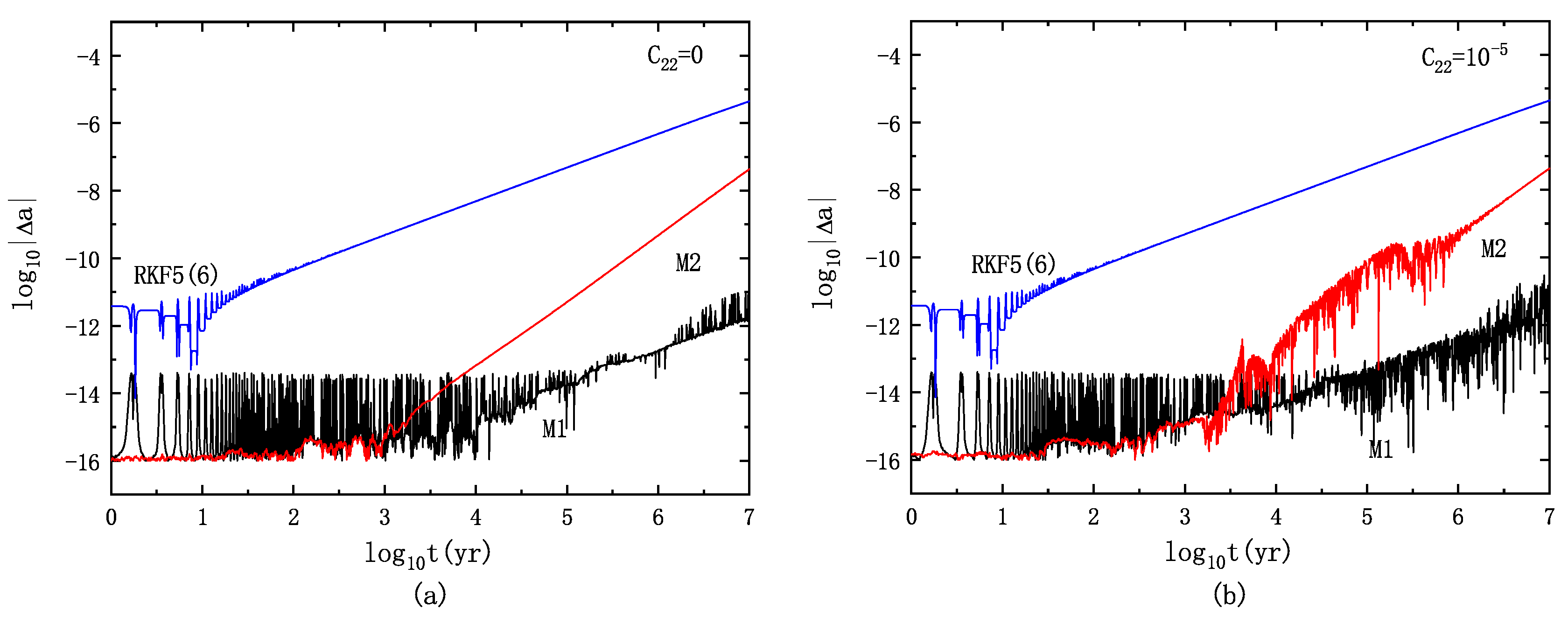
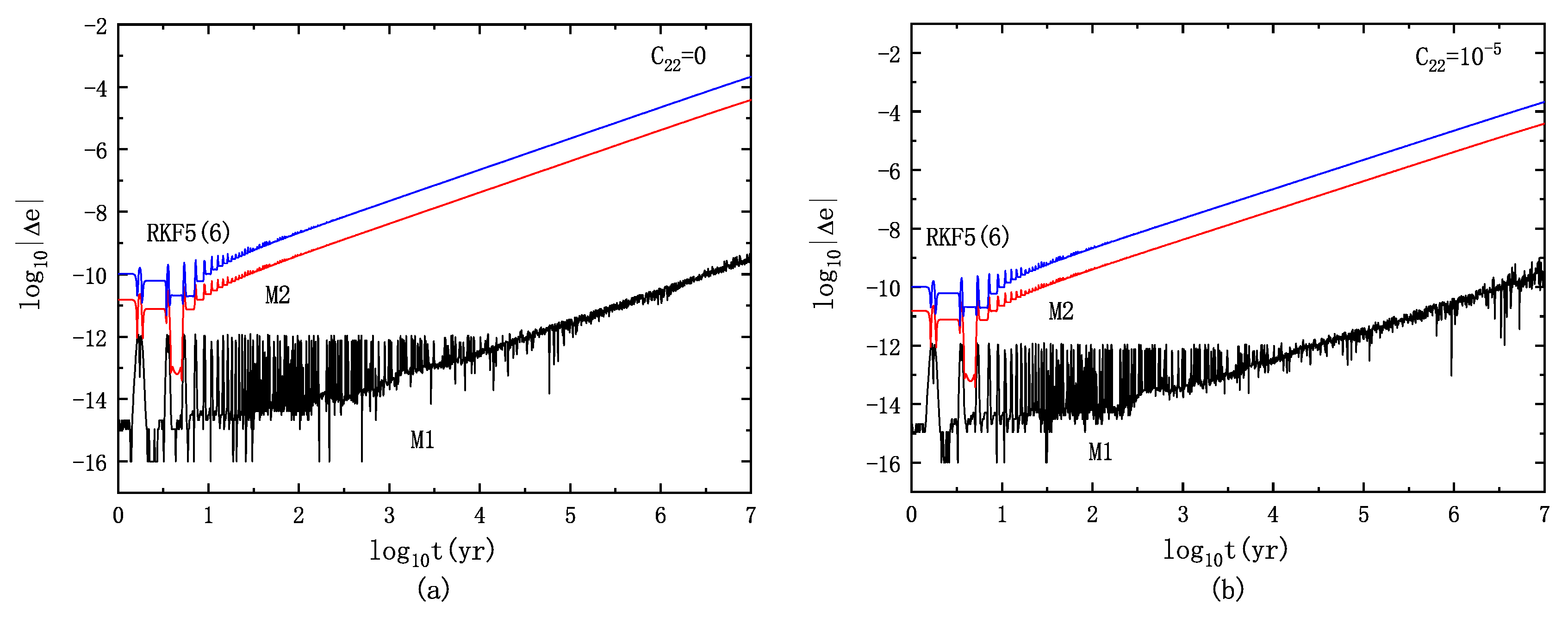
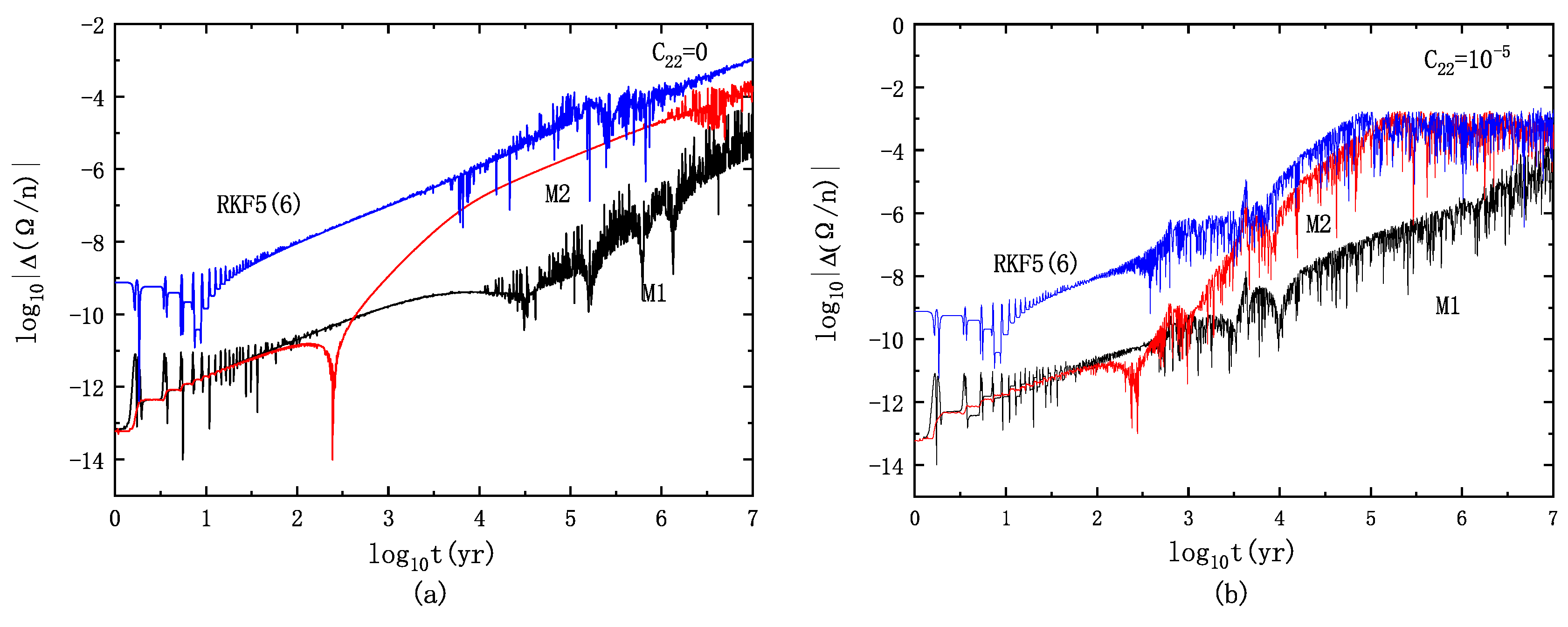
The total angular momentum of the system is composed of two parts: the orbital component and the rotational component. The orbital angular momentum is $m\sqrt{G(m+M)}\sqrt{a(1-e^2)}$. The rotational momentum is contributed by the planet and its host star $C\mathrm{\Omega }\approx {\xi }_1{m}_1{R}_1^2{\mathrm{\Omega }}_1+{\xi }_0{m}_0{R}_0^2{\mathrm{\Omega }}_0$. In this paper, because we only consider the planetary tides, the angular velocity of the planet ${\mathrm{\Omega }}_1$ varies with time, and the angular velocity of the star ${\mathrm{\Omega }}_0$ is approximated as a constant [60]. When $\mathrm{\Omega }\approx n$, it can be proven by Kepler’s third law that the ratio of the rotational component and the orbital component is of the order of ${(R/a)}^2$ [16]. If $R\ll a$, the contribution of the rotational component can be neglected. We get

$$\begin{array}{c}\hfill e_{ini}\simeq \sqrt{1-\frac{a_{current}}{a_{ini}(1-e_{current}^2)}}.\end{array}$$

(30)

The subscript “ini” represents the initial orbital element, and “current” represents the current orbital elements of the planet. Based on the angular momentum of the exoplanets at present, the initial configurations can be derived.

4.2. Numerical Test

Before the numerical simulation, we reproduce the evolution of Kepler-10b in the study of Rodríguez [60]. GJ486 b is a close-in planet with a period of 1.467 days. The physical parameters and detected orbital elements of the planet are shown in

Table 1. Parameters related to planet GJ486 b.

$System$	$\mathit{M}\left({\mathit{m}}_{⨀}\right)$	$\mathit{m}\left({\mathit{m}}_{⨁}\right)$	$\mathit{R}\left({\mathit{R}}_{⨁}\right)$	${\mathit{a}}_{current}$(au)	${\mathit{e}}_{current}$
$GJ486b$	0.32	2.82	1.305	0.01734	0.05

Note: $m_{⨀}$ is the mass of the Sun, $m_{⨁}$ is the mass of the Earth, and $R_{⨁}$ is the radius of the Earth.

. The mass and radius of this planet are 2.82$m_{⨁}$ and 1.305$R_{⨁}$, respectively. The planet is rocky which can be considered as a super-Earth.

We set the initial value of the semimajor axis as $a_{ini}=0.02au$, and $e_{ini}=0.3677$ can be obtained through Equation (30). In addition, we set ${\mathrm{\Omega }}_{ini}=2.7n_{ini}$. For rocky planets such as super-Earths, $\xi =0.25$, and $Q^{\prime }=100$. The RKF5(6) with a fixed time step h being $1/200$ of the orbital period is used as the basic integrator. Because there is no analytical solution for this model, we take the solution calculated by the high-precision eighth- and ninth-order Runge–Kutta–Fehlberg algorithm [RKF8(9)] with variable step sizes as the reference solution for comparison. In the following, we use the high-precision reference solutions calculated by RKF8(9) to calculate the values of $▵a$, $▵e$, and $▵(\mathrm{\Omega }/n)$. Figure 1 shows the errors of the semimajor axis calculated by RKF5(6), the linear transformation method (M1), and the velocity scaling method (M2). Compared to the basic integrator RKF5(6), M1 and M2 significantly improve the accuracy of the semimajor axis. Before $t={10}^3$, the errors of a are reduced by four orders of magnitude. After $t={10}^3$, unlike the previous errors that oscillate within a certain range, $▵a$ increases linearly. The main reason is the long-term accumulation of roundoff errors over time. In addition, we consider the results calculated by RKF8(9) as reference solutions. Because its truncation error and machine roundoff error also accumulate over time, the errors of $▵a$ we get on this basis also increase. In conclusion, we find that the performance of M1 is much better than M2.

The tidal force has influences on the orbital circularization. so it is very important to select an algorithm with better eccentricity accuracy to numerically simulate the process of the tidal evolution. In Figure 2, the performances of the RKF5(6), M1, and M2 algorithms in eccentricity error are exhibited. Compared to the basic integrator RKF5(6), M1 significantly improves the accuracy of eccentricity and works better than M2. M2 only corrects the semi-major axis which is related to the Kepler energy. Because M1 corrects the Laplace integral $\mathit{P}$, the accuracy of eccentricity is improved. Fukushima’s linear transformation method M1 is stable until $t={10}^4$. After that, the accumulated roundoff errors are larger than the truncation errors, and the eccentricity error calculated by M1 begins to increase linearly. The eccentricity error of RKF5(6) without any improvement grows almost linearly with time.

In addition to orbital circularization, the tidal force also has an important effect on the rotation of the planet. Figure 3 displays the errors of $\mathrm{\Omega }/n$ for RKF5(6), M1, and M2. M1 and M2 improve the accuracy of the semimajor axis by correcting the Kepler energy, and the mean motion is $n=\sqrt{\mu /a^3}$. Compared to the uncorrected basic integrator RKF5(6), M1 improves the accuracy of $\mathrm{\Omega }/n$ by approximately four orders of magnitude. Thereafter, although the accuracy of M2 is still an order of magnitude higher than RKF5(6), M1’s accuracy is still the best among them, higher than both M1 and RKF5(6).

Figure 4 shows the evolution of $\mathrm{\Omega }/n$ over time for GJ486 b. For the presence of the gravitational force and torque generated by the asymmetric deformation $(C_{22}={10}^{-5})$, the ratio of planetary angular rotation velocity to the mean motion soon dropped to $\mathrm{\Omega }/n=3/2$, at this point the planetary rotation is captured in $3/2$ spin-orbit resonance. At about 800 Kyr, the ratio drops to $\mathrm{\Omega }/n=1$, and the rotation escapes from the $3/2$ spin-orbit resonance, then enters into $1/1$ spin-orbit resonance and synchronous motion are captured. When only the tidal forces act $(C_{22}=0)$, numerical experiments show that the synchronization is achieved around 2250 Kyr. It follows that the time to achieve synchronization is shortened because of the introduction of planetary equatorial asymmetry.

M1 performs best in the accuracy of the orbital semimajor axis. In Figure 5, we show the orbital evolutions in two cases: one is the action of only tidal forces, and the other is the combined action of tidal forces and the gravitational force generated by the asymmetric deformation of the planet. When deformation forces are present $(C_{22}={10}^{-5})$, GJ486 b is captured by nonsynchronous resonant motion and the rate of variations of the semimajor axis is larger than which in the case of the pure tidal $(C_{22}=0)$. The semimajor axis first evolved in the 3/2 trapping and then the rotation toward a synchronization between the rotation and orbital motions.

As shown above, M1 performs well in the semimajor axis and eccentricity errors. We select the linear transformation method to numerically simulate the tidal evolution and analyze the influences of tidal and the gravitational force generated by the asymmetric deformation on eccentricity. In Figure 6, the rate of variations of eccentricity is larger when deformable forces are present $(C_{22}={10}^{-5})$. The nonsynchronous resonant motion accelerates the rate of eccentricity dissipation when both tidal and deformation forces are present. It is worth noting that in the case of $C_{22}={10}^{-5}$, $1/1$ spin-orbit resonance can be captured at about 800 Kyr when $e\approx 0.05$. This shows that synchronous motion can be captured even for $e\ne 0$ [60]. It was also confirmed that for eccentric orbits, the synchronous motion can occur when there is an additional torque that can counteracts the tidal torque [8,60,69].

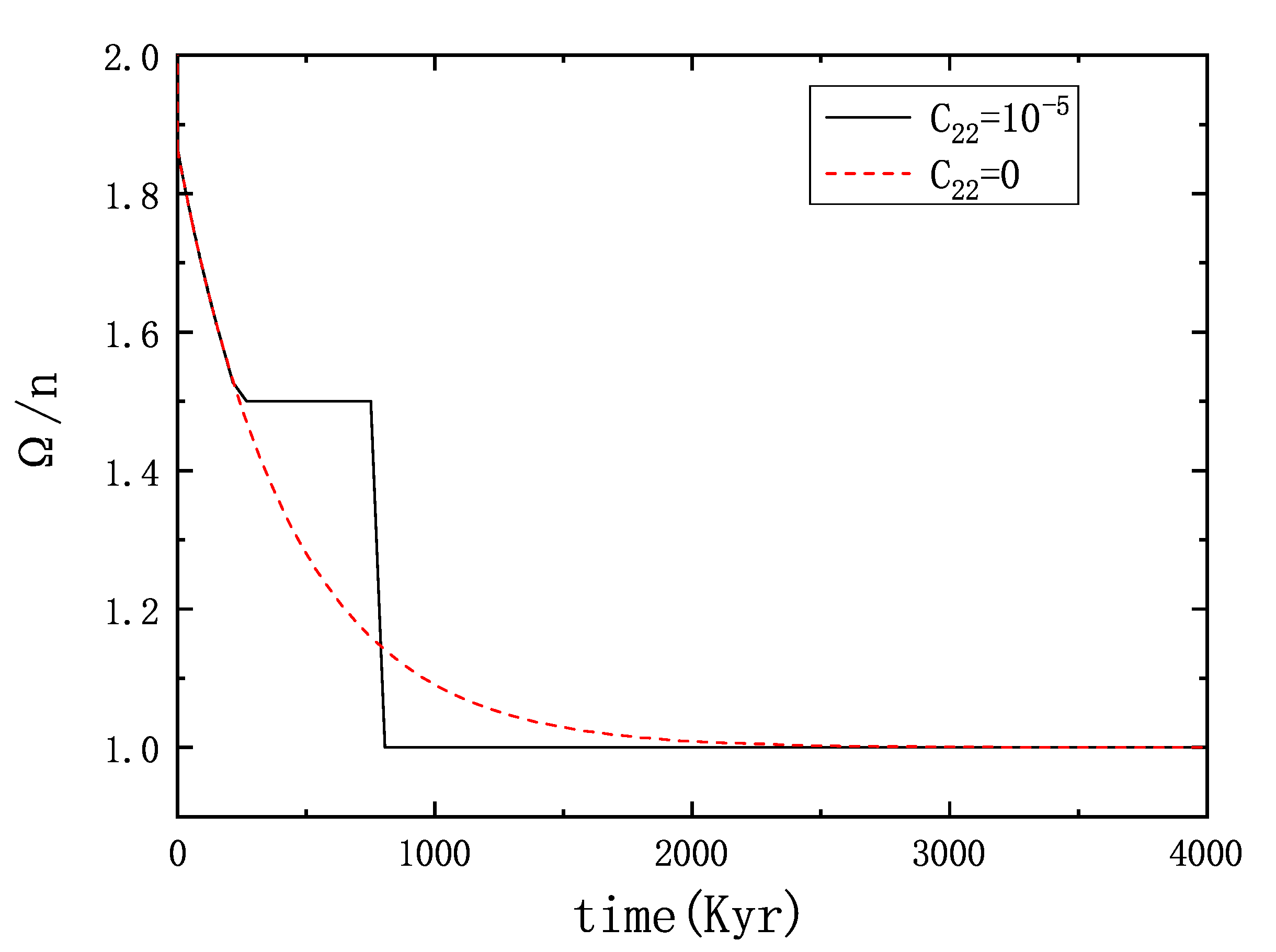
4.3. Tidal Evolution Timescale

We filter several super-Earths (2-4$R_{⨁}$, 1-10$m_{⨁}$, T < 10 days) and then remove the ones with missing datas of semimajor axis and eccentricity. Currently, there are 10 super-Earth systems with complete data in close-in spin-orbit resonance. We use the optimal algorithm obtained in the article to predict the timescale of a series of super-Earths from the current state to synchronous rotation. Under the perturbation of the planetary tidal effect, the tidal timescale is derived from the averaged equations over a period of orbital motion [22]:

$$\begin{array}{c}\hfill {\tau }_{tide}=\frac{4Q^{\prime }}{63n}\frac{m}{M}{\left(\frac{a}{R}\right)}^5.\end{array}$$

(31)

For super-Earths, also known as mini-Neptunes, we take Neptune’s rotation rate as the initial value of the planet’s rotation rate and the tidal quality factor $Q^{\prime }=100$. Then, uncorrected RKF5(6) and Fukushima’s linear transformation method are used to numerically simulate the timescale of a series of super-Earths from the current state to 1/1 spin-orbit resonances. The relevant physical parameters of these super-Earths are shown in

Table 2. The physical parameters of super-Earths.

$Planet$	$\mathit{M}\left({\mathit{m}}_{⨀}\right)$	$\mathit{m}\left({\mathit{m}}_{⨁}\right)$	$\mathit{R}\left({\mathit{R}}_{⨁}\right)$	T (Day)	a (au)	e
GJ3090 b	0.52	3.34	2.13	2.85	0.032	0.32
HD110113 b	1	4.55	2.05	2.54	0.035	0.093
TOI-2136 b	0.33	4.7	2.2	7.85	0.053	0.07
K2-146 b	0.36	5.6	2.25	2.67	0.025	0.14
TOI-125 c	0.86	6.63	2.76	9.15	0.081	0.066
K2-146 c	0.36	7.1	2.59	3.97	0.033	0.16
HD 86226 c	1.02	7.25	2.16	3.98	0.049	0.075
HD 97658 b	0.75	7.86	2.34	9.49	0.0796	0.063
TOI-269 b	0.39	8.8	2.77	3.70	0.0345	0.425
TOI-125 b	0.86	9.5	2.73	4.65	0.052	0.194

. The calculated results are shown in

Table 3. Timescale of tidal evolution of planetary systems.

Planet	τ0 (yr)	|Δτ0| (yr)	τ1 (yr)	|Δτ1| (yr)	τ (yr)
GJ3090 b	$2.01\times {10}^6$	$1.22\times {10}^6$	$3.35\times {10}^5$	$4.60\times {10}^5$	$7.95\times {10}^5$
HD 110113 b	$1.48\times {10}^6$	$5.35\times {10}^5$	$1.27\times {10}^6$	$3.25\times {10}^5$	$9.45\times {10}^5$
TOI-2136 b	$8.74\times {10}^6$	$4.70\times {10}^7$	$7.25\times {10}^7$	$1.68\times {10}^7$	$5.57\times {10}^7$
K2-146 b	$7.69\times {10}^6$	$4.09\times {10}^5$	$7.69\times {10}^5$	$4.09\times {10}^5$	$3.60\times {10}^5$
TOI-125 c	$1.74\times {10}^7$	$7.70\times {10}^7$	$2.26\times {10}^7$	$7.18\times {10}^7$	$9.44\times {10}^7$
K2-146 c	$6.14\times {10}^6$	$4.78\times {10}^6$	$8.57\times {10}^6$	$7.21\times {10}^6$	$1.36\times {10}^6$
HD 86226 c	$2.87\times {10}^7$	$1.87\times {10}^7$	$1.31\times {10}^7$	$0.31\times {10}^7$	$1.00\times {10}^7$
HD 97658 b	$1.01\times {10}^8$	$1.69\times {10}^8$	$2.74\times {10}^8$	$0.04\times {10}^8$	$2.70\times {10}^8$
TOI-269 b	$1.76\times {10}^6$	$0.24\times {10}^6$	$6.16\times {10}^6$	$4.64\times {10}^6$	$1.52\times {10}^6$
TOI-125 b	$4.29\times {10}^6$	$3.38\times {10}^6$	$4.94\times {10}^6$	$2.73\times {10}^6$	$7.67\times {10}^6$

, where $\tau$ represents the results of theoretical calculations; ${\tau }_0$ represents the calculation result of RKF5(6); ${\tau }_1$ represents the calculation results of Fukushima’s manifold correction methods; $\left|\Delta \tau \right|$ represents the difference from the theoretical calculation. The RKF5(6) and Fukushima’s manifold correction methods are different from the theoretical values calculated by Equation (31), but in most cases $|\Delta {\tau }_1|<|\Delta {\tau }_0|$. It can be seen that the numerical simulation by using the Fukushima’s method is closer to the theoretical value, and the applicability of the manifold correction algorithm in the two-body problem of tidal model is verified.

5. Summary and Outlook

In this paper, the manifold correction methods are applied to the tidal evolution of the exoplanet. GJ486 b, a short-period super-Earth, is used to analyze the accuracies of the parameters of the velocity scaling method and the Fukushima’s linear transformation method in the tidal evolution process. We also analyzed the coupled spin-orbit evolution of GJ486 b. Numerical experiments show that, compared with the uncorrected basic integrator RKF5(6), the velocity scaling method can improve the precision of the semimajor axis by correcting the velocity obtained from the integral of each step. The accuracy of the linear transformation method is better than that of RKF5(6) and the velocity scaling method in the semimajor axis, eccentricity, and the ratio of planetary angular rotation velocity to mean motion. Through numerical simulation, resonance can be captured during exoplanet evolution when deformation forces and torques are present, such as 3/2 and 1/1 spin-orbit resonances. The decrease in eccentricity caused by the tide will destabilize the current higher-order spin-orbit resonances out of the current configuration and into the lower-order spin-orbit resonances [70,71]. When only tidal forces are present, no resonance is captured during the exoplanet evolution, and it takes more time to reach a tidally locked state. Tidal force makes the planetary orbit decay and circularization. In the presence of gravitational and tidal torques, the planet will be captured by the spin-orbit resonance, and accelerate the evolution to reach the synchronous spin-orbit resonance.

Compared with the RKF5(6), both manifold correction methods used in the tidal model have improved the accuracy in the semimajor axis, eccentricity, and the ratio of planetary rotation angular velocity to the mean motion. Simulation of the evolution of exoplanets with tides force requires a stable and high-accuracy integration to ensure the reliability of the results. In this work, we consider the model of a single planetary system. The research on the tidal effect of a multiplanet system with more than two planets is more complicated [13,15,21,22,23] because of the coupling effect between the gravitational forces of the planets and the tidal effects. We will pay more attention to the exoplanets of binary planetary systems in the future.

References

1. Mayor, M.; Queloz, D. A Jupiter-mass companion to a solar-type star. Nature 1995, 378, 355–359. [Google Scholar] [CrossRef]
2. Rasio, F.A.; Tout, C.A.; Lubow, S.H.; Livio, M. Tidal decay close planetary orbits. Astrophys. J. 1996, 470, 1187. [Google Scholar] [CrossRef]
3. Jackson, B.; Greenberg, R.; Barnes, R. Tidal Evolution of Close-in Extrasolar Planets. Astrophys. J. 2008, 678, 1396–1406. [Google Scholar] [CrossRef] [Green Version]
4. Penev, K.; Sasselov, D. Tidal Evolution of Close-in Extrasolar Planets: High Stellar Q from New Theoretical Models. Astrophys. J. 2011, 731, 67. [Google Scholar] [CrossRef] [Green Version]
5. Goldreich, P. On the Eccentricity of Satellite Orbits in the Solar System. Mon. Not. R. Astron. Soc. 1963, 126, 257. [Google Scholar] [CrossRef] [Green Version]
6. Goldreich, P.; Soter, S. Q in the solar system. Icarus 1966, 5, 375–389. [Google Scholar] [CrossRef]
7. Mardling, R.A.; Lin, D.N.C. Calculating the Tidal, Spin, and Dynamical Evolution of Extrasolar Planetary Systems. Astrophys. J. 2002, 573, 829–844. [Google Scholar] [CrossRef]
8. Ferraz-Mello, S.; Rodríguez, A.; Hussmann, H. Tidal friction in close-in satellites and exoplanets: The Darwin theory re-visited. Celest. Mech. Dyn. Astron. 2008, 101, 171–201. [Google Scholar] [CrossRef]
9. Agnor, C.B.; Canup, R.M.; Levison, H.F. On the Character and Consequences of Large Impacts in the Late Stage of Terrestrial Planet Formation. Icarus 1999, 142, 219–237. [Google Scholar] [CrossRef]
10. Kokubo, E.; Ida, S. Formation of Terrestrial Planets from Protoplanets. II. Statistics of Planetary Spin. Astrophys. J. 2007, 671, 2082–2090. [Google Scholar] [CrossRef]
11. Jackson, B.; Barnes, R.; Greenberg, R. Observational Evidence for Tidal Destruction of Exoplanets. Astrophys. J. 2009, 698, 1357–1366. [Google Scholar] [CrossRef] [Green Version]
12. Jackson, B.; Greenberg, R.; Barnes, R. Tidal Heating of Extrasolar Planets. Astrophys. J. 2008, 681, 1631–1638. [Google Scholar] [CrossRef] [Green Version]
13. Mardling, R.A. Long-term Tidal Evolution of Short-period Planets with Companions. Mon. Not. R. Astron. Soc. 2007, 382, 1768–1790. [Google Scholar] [CrossRef] [Green Version]
14. Pätzold, M.; Carone, L.; Rauer, H. Tidal interactions of close-in extrasolar planets: The OGLE cases. Astron. Astrophys. 2004, 427, 1075–1080. [Google Scholar] [CrossRef] [Green Version]
15. Mardling, R.A. The determination of planetary structure in tidally relaxed inclined systems. Mon. Not. R. Astron. Soc. 2010, 407, 1048–1069. [Google Scholar] [CrossRef] [Green Version]
16. Rodríguez, A.; Ferraz-Mello, S.; Michtchenko, T.A. Tidal Decay Orbital Circ. Close-Two-Planet Systems. Mon. Not. R. Astron. Soc. 2011, 415, 2349–2358. [Google Scholar] [CrossRef] [Green Version]
17. Darwin, G.H. The Scientific Papers of Sir George Darwin: Tidal Friction and Cosmogony; Cambridge University Press: Cambridge, UK, 1908; Volume 2. [Google Scholar]
18. MacDonald, G.J.F. Tidal Friction. Rev. Geophys. 1964, 2, 467–541. [Google Scholar] [CrossRef]
19. Kaula, W.M. Tidal Dissipation by Solid Friction and the Resulting Orbital Evolution. Rev. Geophys. 1964, 2, 661–685. [Google Scholar] [CrossRef]
20. Goldreich, P. Final spin states of planets and satellites. Astrophys. J. 1966, 71, 1. [Google Scholar] [CrossRef]
21. Wu, Y.; Goldreich, P. Tidal Evolution of the Planetary System around HD 83443. Astrophys. J. 2002, 564, 1024–1027. [Google Scholar] [CrossRef]
22. Zhou, J.-L.; Lin, D.N.C. Migration and Final Location of Hot Super Earths in the Presence of Gas Giants. Proc. Int. Astron. Union 2008, 249, 285–291. [Google Scholar]
23. Laskar, J.; Boué, G.; Correia, A.C.M. Tidal dissipation in multi-planet systems and constraints on orbit fitting. Astron. Astrophys. 2012, 538, A105. [Google Scholar] [CrossRef]
24. Darwin, G.H. The Determination of the Secular Effects of Tidal Friction by a Graphical Method. Proc. R. Soc. Lond. 1879, 29, 168–181. [Google Scholar]
25. Deng, C.; Wu, X.; Liang, E. The use of Kepler solver in numerical integrations of quasi-Keplerian orbits. Mon. Not. R. Astron. Soc. 2020, 496, 2946–2961. [Google Scholar] [CrossRef]
26. Feng, K. On Differential Geometry and Differential Equations; Science Press: Beijing, China, 1985; Volume 42. [Google Scholar]
27. Ruth, R.D. A Canonical Integration Technique. ITNS 1983, 30, 2669. [Google Scholar]
28. Wang, Y.; Sun, W.; Liu, F.; Wu, X. Construction of Explicit Symplectic Integrators in General Relativity. I. Schwarz. Black Holes. Astrophys. J. 2021, 907, 66. [Google Scholar] [CrossRef]
29. Wang, Y.; Sun, W.; Liu, F.; Wu, X. Construction of Explicit Symplectic Integrators in General Relativity. II. Reissner-Nordström Black Holes. Astrophys. J. 2021, 909, 22. [Google Scholar] [CrossRef]
30. Wang, Y.; Sun, W.; Liu, F.; Wu, X. Construction of Explicit Symplectic Integrators in General Relativity. III. Reissner-Nordström-(anti)-de Sitter Black Holes. Astrophys. J. 2021, 254, 8. [Google Scholar] [CrossRef]
31. Wu, X.; Wang, Y.; Sun, W.; Liu, F. Construction of Explicit Symplectic Integrators in General Relativity. IV. Kerr Black Holes. Astrophys. J. 2021, 914, 63. [Google Scholar] [CrossRef]
32. Wu, X.; Wang, Y.; Sun, W.; Liu, F.-Y.; Han, W.-B. Explicit Symplectic Methods in Black Hole Spacetimes. Astrophys. J. 2022, 940, 166. [Google Scholar] [CrossRef]
33. Pihajoki, P. Explicit methods in extended phase space for inseparable Hamiltonian problems. Celest. Mech. Dyn. Astron. 2015, 121, 211–231. [Google Scholar] [CrossRef] [Green Version]
34. Luo, J.; Wu, X.; Huang, G.; Liu, F. Explicit Symplectic-like Integrators with Midpoint Permutations for Spinning Compact Binaries. Astrophys. J. 2017, 834, 64. [Google Scholar] [CrossRef]
35. Li, D.; Wu, X. Chaotic motion of neutral and charged particles in a magnetized Ernst-Schwarzschild spacetime. Eur. Phys. J. Plus 2019, 134, 96. [Google Scholar] [CrossRef]
36. Hu, S.; Wu, X.; Huang, G. A Novel Energy-conserving Scheme for Eight-dimensional Hamiltonian Problems. Astrophys. J. 2019, 887, 191. [Google Scholar] [CrossRef] [Green Version]
37. Hu, S.; Wu, X.; Liang, E. An Energy-conserving Integrator for Conservative Hamiltonian Systems with Ten-dimensional Phase Space. Astrophys. J. Suppl. Ser. 2021, 253, 55. [Google Scholar] [CrossRef]
38. Hu, S.; Wu, X.; Liang, E. Construction of a Second-order Six-dimensional Hamiltonian-conserving Scheme. Astrophys. J. Suppl. Ser. 2021, 257, 40. [Google Scholar] [CrossRef]
39. Zhong, S.-Y.; Wu, X.; Liu, S.-Q.; Deng, X.-F. Global symplectic structure-preserving integrators for spinning compact binaries. Phys. Rev. D 2010, 82, 124040. [Google Scholar] [CrossRef]
40. Mei, L.; Wu, X.; Liu, F. On preference of Yoshida construction over Forest-Ruth fourth-order symplectic algorithm. Eur. Phys. J. C 2013, 73, 2413. [Google Scholar] [CrossRef]
41. Mei, L.; Ju, M.; Wu, X.; Liu, S. Dynamics of spin effects of compact binaries. Mon. Not. R. Astron. Soc. 2013, 435, 2246–2255. [Google Scholar] [CrossRef] [Green Version]
42. Huang, G.; Ni, X.; Wu, X. Chaos in two black holes with next-to-leading order spin-spin interactions. Eur. Phys. J. C 2014, 74, 3012. [Google Scholar] [CrossRef] [Green Version]
43. Huang, L.; Wu, X.; Ma, D. Second post-Newtonian Lagrangian dynamics of spinning compact binaries. Eur. Phys. J. C 2016, 76, 4339. [Google Scholar] [CrossRef] [Green Version]
44. Ma, D.-Z.; Wu, X.; Zhong, S.-Y. Extending Nacozy’s Approach to Correct All Orbital Elements for Each of Multiple Bodies. Astrophys. J. 2008, 687, 1294–1302. [Google Scholar] [CrossRef] [Green Version]
45. Zhong, S.-Y.; Wu, X. A velocity scaling method with least-squares correction of several constraints. Astrophys. Space Sci. 2009, 324, 31–40. [Google Scholar] [CrossRef]
46. Zhong, S.-Y.; Wu, X. Manifold corrections on spinning compact binaries. Phys. Rev. D 2010, 81, 104037. [Google Scholar] [CrossRef]
47. Mei, L.-J.; Wu, X.; Liu, F.-Y. A New Class of Scaling Correction Methods. Chin. Phys. Lett. 2012, 29, 050201. [Google Scholar] [CrossRef]
48. Wang, S.-C.; Wu, X.; Liu, F.-Y. Implementation of the velocity scaling method for elliptic restricted three-body problems. Mon. Not. R. Astron. Soc. 2016, 463, 1352–1362. [Google Scholar] [CrossRef]
49. Wang, S.; Huang, G.; Wu, X. Simulations of Dissipative Circular Restricted Three-body Problems Using the Velocity-scaling Correction Method. Astrophys. J. 2018, 155, 67. [Google Scholar] [CrossRef]
50. Nacozy, P.E. The Use of Integrals in Numerical Integrations of the N-Body Problem. Astrophys. Space Sci. 1971, 14, 40–51. [Google Scholar] [CrossRef]
51. Baumgarte, J. Numerical Stabilization of the Differential Equations of Keplerian Motion. Celest. Mech. 1972, 5, 490–501. [Google Scholar] [CrossRef]
52. Liu, L.; Liao, X. Numerical Calculations in the Orbital Determination of an Artificial Satellite for a Long Arc. Celest. Mech. Dyn. Astron. 1994, 59, 221–235. [Google Scholar] [CrossRef]
53. Liu, L.; Liao, X. On several problems in the numerical integration of celestial orbits. Chin. Astron. Astrophys. 1988, 12, 26–33. [Google Scholar] [CrossRef]
54. Fukushima, T. Efficient Orbit Integration by Scaling for Kepler Energy Consistency. Astrophys. J. 2003, 126, 1097–1111. [Google Scholar] [CrossRef] [Green Version]
55. Ma, D.-Z.; Wu, X.; Zhu, J.-F. Velocity scaling method to correct individual Kepler energies. New Astron. 2008, 13, 216–223. [Google Scholar] [CrossRef]
56. Fukushima, T. Efficient Orbit Integration by Dual Scaling for Consistency of Kepler Energy and Laplace Integral. Astrophys. J. 2003, 126, 2567–2573. [Google Scholar] [CrossRef]
57. Wu, X.; Huang, T.-Y.; Wan, X.-S.; Zhang, H. Comparison among Correction Methods Individ. Kepler Energies N-Body Simulations. Astrophys. J. 2007, 133, 2643–2653. [Google Scholar]
58. Fukushima, T. Efficient Orbit Integration by Scaling and Rotation for Consistency of Kepler Energy, Laplace Integral, and Angular Momentum Direction. Astrophys. J. 2003, 126, 3138–3142. [Google Scholar] [CrossRef]
59. Fukushima, T. Efficient Orbit Integration by Linear Transformation for Consistency of Kepler Energy, Full Laplace Integral, and Angular Momentum Vector. Astrophys. J. 2004, 127, 3638–3641. [Google Scholar] [CrossRef]
60. Rodríguez, A.; Callegari, N.; Michtchenko, T.A.; Hussmann, H. Spin-Orbit Coupling Tidally Evol. Super-Earths. Mon. Not. R. Astron. Soc. 2012, 427, 2239–2250. [Google Scholar] [CrossRef] [Green Version]
61. Mignard, F. The Evolution of the Lunar Orbit Revisited. I. Moon Planets 1979, 20, 301–315. [Google Scholar] [CrossRef]
62. Darwin, G.H. On the Secular Changes in the Elements of the Orbit of a Satellite Revolving about a Tidally Distorted Planet. Philos. Trans. 1880, 171, 713–891. [Google Scholar]
63. Beutler, G. Methods of Celestial Mechanics; Springer: Berlin, Germany, 2005; Volume 102. [Google Scholar]
64. Danby, J. Fundamentals of celestial mechanics. In Astrophysics and Space Science; Macmillan: New York, NY, USA, 1962. [Google Scholar]
65. Millholland, S.; Laughlin, G. Obliquity Tides May Drive WASP-12b’s Rapid Orbital Decay. Astrophys. J. 2018, 869, 1. [Google Scholar] [CrossRef]
66. Li, Q.; Wang, N.; Yi, D. Numerical Analysis; Tsinghua University Press: Beijing, China, 2001. [Google Scholar]
67. Deng, J.; Liu, Z. Calculation Method; Xi’an Jiaotong University Press: Xi’an, China, 2001. [Google Scholar]
68. Fukushima, T. Efficient Integration of Highly Eccentric Orbits by Scaling Methods Applied to Kustaanheimo-Stiefel Regularization. Astrophys. J. 2004, 128, 3114. [Google Scholar] [CrossRef] [Green Version]
69. Goldreich, P.; Peale, S. Spin-orbit coupling in the solar system. Astrophys. J. 1966, 71, 425. [Google Scholar] [CrossRef]
70. Correia, A.C.M.; Laskar, J. Mercury’s capture into the 3/2 spin-orbit resonance as a result of its chaotic dynamics. Nature 2004, 429, 848–850. [Google Scholar] [CrossRef]
71. Correia, A.C.M.; Laskar, J. Mercury’s capture into the 3/2 spin-orbit resonance including the effect of core-mantle friction. Icarus 2009, 201, 1–11. [Google Scholar] [CrossRef]
Figure 1. The error map of the semimajor axis of GJ486b in the process of planetary evolution. The algorithms involved in the figure are RKF5(6), Fukushima’s linear transformation method(M1), and velocity scaling method(M2). (a) C 22 = 0 , only tidal effects exist; (b) C 22 = 10 5 , tidal and deformation forces and torques exist at the same time.
Symmetry 15 00253 g001
Figure 2. Eccentricity error map of GJ486 b during planetary evolution. The algorithms used are RKF5(6), Fukushima’s linear transformation method(M1), and velocity scaling(M2). (a) C 22 = 0 , only tidal effects exist; (b) C 22 = 10 5 , tidal and deformation forces and torques exist at the same time.
Symmetry 15 00253 g002
Figure 3. Error map of the ratio of the angular rotation velocity to the mean motion of GJ486 b during planetary evolution. The algorithms used are RKF5(6), Fukushima’s linear transformation method(M1), and velocity scaling(M2). (a) C 22 = 0 , only tidal effects exist; (b) C 22 = 10 5 , tidal and deformation forces and torques exist at the same time.
Symmetry 15 00253 g003
Figure 4. Time variation of Ω / n for GJ486 b. Different evolutions were observed, including capturing 3 / 2 and 1 / 1 spin-orbit resonances. The dotted line corresponds to the presence of only the tidal effect, and the solid line corresponds to the coexistence of tidal and deformation forces and torques. These evolutionary results are calculated from M1.
Symmetry 15 00253 g004
Figure 5. Evolution of the semimajor axis of GJ486 b over time. The variable rates of a are different when the rotation is trapped in different capture. These evolutionary results are calculated from M1.
Symmetry 15 00253 g005
Figure 6. Eccentricity evolution of GJ486 b over time. The rate of change of e depends on the specific capture in which the spin is trapped. When the rotation is in resonance, the eccentricity changes rapidly. These evolutionary results are calculated from M1.
Symmetry 15 00253 g006