Study of Chaos in Rotating Galaxies Using Extended Force-Gradient Symplectic Methods

Abstract

We take into account the dynamics of three types of models of rotating galaxies in polar coordinates in a rotating frame. Due to non-axisymmetric potential perturbations, the angular momentum varies with time, and the kinetic energy depends on the momenta and spatial coordinate. The existing explicit force-gradient symplectic integrators are not applicable to such Hamiltonian problems, but the recently extended force-gradient symplectic methods proposed in previous work are. Numerical comparisons show that the extended force-gradient fourth-order symplectic method with symmetry is superior to the standard fourth-order symplectic method but inferior to the optimized extended force-gradient fourth-order symplectic method in accuracy. The optimized extended algorithm with symmetry is used to explore the dynamical features of regular and chaotic orbits in these rotating galaxy models. The gravity effects and the degree of chaos increase with an increase in the number of radial terms in the series expansions of the potential. There are similar dynamical structures of regular and chaotical orbits in the three types of models for the same number of radial terms in the series expansions, energy and initial conditions.

1. Introduction

Chaos in a dynamical system means that the final state of the dynamical system displays exponentially sensitive dependence on the initial state. Based on the importance of chaos, many studies have focused on the subject of chaos in the solar system [1,2] and galactic dynamics [3,4,5,6,7].

Regular or chaotic motions of particles in galactic dynamics may affect the fraction of mass. The authors of Refs. [3,5,6,7] investigated mass components of non-rotating N-body models of elliptical galaxies in ordered and chaotic motion. Voglis et al. [3] found that the fraction of mass in chaotic motion is about 24% of the total mass in one non-rotating triaxial equilibrium model with smooth centers and 32% in another non-rotating triaxial equilibrium model with smooth centers. This shows that the spatial distribution of the mass in chaotic motion is in disagreement with that in ordered motion. Muzzio et al. [7] pointed out that the fraction of mass in chaotic motion of about 53% in models of non-rotating galaxies with smooth centers. On the other hand, the fraction of mass in ordered or chaotic motion was also studied in spiral galaxies. Voglis et al. [8] further showed that rotation leads to increasing the fraction of mass in chaotic motion (up to the level of $\approx 65\%$) and shifting the Lyapunov numbers to larger values in N-body models of rotating galaxies. In other words, the extent of chaos is substantially enhanced by the rotation, and the fractions of mass in chaotic motion in the rotating models are larger than those in the non-rotating models. The spatial distributions of the dynamical structures along the spiral arms at the ends of the bar in the barred-spiral galaxy correspond to those of particles with masses in regular and in chaotic orbits. In fact, the mass in chaotic motion can almost completely form spiral arms emanating from the neighborhood of the Lagrangian points $L_1$ and $L_2$ at the ends of the bar in a barred-spiral galaxy. The distribution of mass must be associated with the gravitational forces of particles. Gravity is the main driving mechanism for the formation and the stability of spiral arms in galaxies. The authors of Refs. [9,10] developed the Moser analytic series representing the invariant manifolds near the unstable Lagrangian equilibrium points $L_1$, $L_2$ in a rotating barred galaxy. In this way, these series can represent the spiral arms, which are density waves and are composed of chaotic orbits. In addition to the analytical theory, other methods such as the specific finite time Lyapunov characteristic number, the smaller alignment index, the surface of section and the frequency analysis were used to classify the orbits in regular and chaotic cases in barred galaxies [11,12,13,14,15].

The onset of chaos in two-dimensional Hamiltonian systems of rotating galaxies in the disc plane in polar coordinates [10] is due to the inclusion of non-axisymmetric potential perturbations. These perturbations cause the angular momentum with respect to the angle to vary with time, and therefore, the Hamiltonian systems are not integrable. This non-integrability leads to chaos under some circumstances. Reliable numerical results are always required to detect the chaotic behavior. In some cases, extremely long integration times are also required. The adopted computational schemes for the long-term integration of the Hamiltonian systems become crucial to reach better stability and higher precision. The proper choice of the integrators should naturally be symplectic schemes, which preserve the symplectic nature of Hamiltonian dynamics [16,17]. Symplectic methods are a class of geometric integration algorithms [18] and make the local error in the total energy not grow with time. There are standard symplectic methods [19,20] that require some evaluations of the force and force-gradient symplectic integrators [16,21,22,23,24] that require some evaluations of force gradient in addition to several evaluations of the force. Because of good long-term behavior, the standard symplectic methods have been used in the solar system [1,25] and black hole spacetimes [26,27,28,29,30,31]. They are also suitable for the two-dimensional Hamiltonian systems of rotating galaxies in polar coordinates. However, the force-gradient symplectic integrators are not applicable to such Hamiltonian problems because the kinetic energies of the Hamiltonian systems depend on the momenta and spatial coordinates. In fact, they are only adapted to the integrations of Hamiltonian systems, where the kinetic energies are quadratic functions of momenta, and the potential energies are functions of coordinates. Energy errors of the force-gradient symplectic integrators are several orders of magnitude smaller than those of the standard symplectic algorithms of the same order, as was confirmed in the literature [22,23,24]. Recently, our group extended these force-gradient integrators to the explicitly integrable kinetic energies, which are not only quadratic functions of momenta but also depend on coordinates [32]. When the original force-gradient operator is adjusted appropriately, the adjusted operator lacks the concept of force gradient and belongs to the momentum operator, such as the operator corresponding to the potential. As a result, the existing explicit force-gradient symplectic integrators [21,22,23,24] are still available in the extended Hamiltonian systems. The extended force-gradient symplectic integrators do not alter their symmetry and time reversibility compared with the existing force-gradient algorithms. The authors of Ref. [32] used a modified Hénon-Heiles system and a spring pendulum as two toy models to test the numerical performance of the extended algorithms. They showed that the fourth-order Forest–Ruth standard symplectic method does not give true dynamical properties of order and chaos to the modified Hénon–Heiles system under some circumstances, whereas the fourth-order extended force-gradient symplectic methods do. The obtained results are because the Forest–Ruth method performs with poorer accuracy than the extended force-gradient algorithms. In fact, the optimized fourth-order extended force-gradient symplectic methods have energy errors that are three orders of magnitude smaller than those of the Forest–Ruth method.

Note that the extended force-gradient symplectic methods proposed in Ref. [32] were shown to have good numerical performance in the simulations of the two toy models. Now, we wonder whether the extended algorithms still exhibit excellent performance in the application of real astronomical and astrophysical problems. Evaluating the performance of the extended force-gradient symplectic methods applicable to the three types of models of rotating barred galaxies in Refs. [8,10] is one of the main aims of the present paper. On the other hand, we are interested in studying a distribution of dynamical structures regarding regular and chaotic orbits along the radial direction for a given number of the radial terms of the potential in one of the models using the techniques of the Poincaré surface of section and fast Lyapunov indicators (FLIs) [33]. In this way, we desire to know how the number of the radial terms of the potential affects chaos in one of the models. We also desire to know what differences in the dynamics exist among the three types of models with the same number of radial terms of the potential, energy and initial conditions.

To implement the three aims, we organize this paper as follows. In Section 2, we introduce three types of models of rotating barred galaxies. In Section 3, we apply the extended fourth-order force-gradient symplectic methods to Model A4 and evaluate the performance of these algorithms. In Section 4, we explore the dynamical structures in these models using the techniques of the Poincaré surface of section and FLIs. Finally, the main results are summarized in Section 5.

2. Models of Rotating Barred Galaxies

The motion of a test particle of mass $m_p=1$ in the plane of a galaxy with a rotating bar is described in polar coordinates $(r,\varphi )$ in the rotating frame by a two-dimensional Hamiltonian [8,10]

$$H=\frac{p_r^2}{2}+\frac{p_{\varphi }^2}{2r^2}-\Omega p_{\varphi }+\Phi (r,\varphi ).$$

(1)

The above notations are given here. $\Omega$ is a pattern speed of the rotating frame. $p_r$ represents the canonical momentum vs. the coordinate r, and $p_{\varphi }$ is the canonical momentum of the coordinate $\varphi$ corresponding to the angular momentum in the rest frame. $\Phi (r,\varphi )$ denotes the gravitational potential of the galaxy in the rotating frame and satisfies the Poisson equation

$${\nabla }^2\Phi =4\pi G\rho ,$$

(2)

where G is the constant of gravity, and $\rho$ stands for the density of matter.

A complete expression of the solution of the Poisson equation is long and complicated. Harsoula et al. [10] took a simple solution of Equation (2) as the potential for the $m=2$ mode of the galactic bar

$$\Phi (r,\varphi )={\Phi }_0\left(r\right)+{\Phi }_1\left(r\right)cos2\varphi +{\Phi }_2\left(r\right)sin2\varphi ,$$

(3)

where ${\Phi }_0\left(r\right)$, ${\Phi }_1\left(r\right)$ and ${\Phi }_2\left(r\right)$ are functions of r. If ${\Phi }_1\left(r\right)={\Phi }_2\left(r\right)=0$, then the potential ${\Phi }_0\left(r\right)=\Phi (r,\varphi )$ is axisymmetric and the angular momentum $p_{\varphi }$ is conserved. When ${\Phi }_1\left(r\right)\ne 0$ or ${\Phi }_2\left(r\right)\ne 0$, the potential $\Phi (r,\varphi )$ is non-axisymmetric and the angular momentum $p_{\varphi }$ is not conserved. Namely, the second and third terms of Equation (3) act as an $m=2$ mode of the non-axisymmetric potential perturbation. The three potential functions are given in Ref. [10] by

$$\begin{array}{ccc}& & \hspace{1em}\hspace{1em}\hspace{1em}\hspace{1em}\hspace{1em}\hspace{1em} {\Phi }_0\left(r\right)=-\frac{1}{R}\left(A_{00}+\frac{1}{4}{A}_{20}-\frac{3}{2}{A}_{22}\right),\hfill \end{array}$$

(4)

$$\begin{array}{ccc}& & \hspace{1em}\hspace{1em}\hspace{1em}\hspace{1em} {\Phi }_1\left(r\right)=-\frac{3}{2R}\left(\frac{1}{2}{A}_{20}+A_{22}\right),\hfill \end{array}$$

(5)

$$\begin{array}{ccc}& & {\Phi }_2\left(r\right)=\frac{3}{2R}{A}_{21},\hfill \end{array}$$

(6)

where R is a numerical constant for the description of the size of the system. The size is regarded as the N-body code boundary corresponding to the solutions of the Poisson equation matched with the solutions of the Laplace equation. The other notations such as $A_{00}$ are expanded in terms of the series of spherical Bessel functions $j_0$ and $j_2$ [34]:

$$\begin{array}{c}\hfill A_{00}=\sum _{i=0}^n\left[B_{i00}·j_0\left({\xi }_{i0}\right)\right],\end{array}$$

(7)

$$\begin{array}{c}\hfill A_{20}=\sum _{i=0}^n\left[B_{i20}·j_2\left({\xi }_{i2}\right)\right],\end{array}$$

(8)

$$\begin{array}{c}\hfill A_{21}=\sum _{i=0}^n\left[C_{i21}·j_2\left({\xi }_{i2}\right)\right],\end{array}$$

(9)

$$\begin{array}{c}\hfill A_{22}=\sum _{i=0}^n\left[B_{i22}·j_2\left({\xi }_{i2}\right)\right].\end{array}$$

(10)

In the above series of expansions of the potential, n represents the number of the radial terms; that is, each of the functions, such as $A_{00}$, in the potential has $(n+1)$ terms. In addition, ${\xi }_{il}=a_{il}r/R$. For $l=0$, $a_{i0}=(i+1/2)\pi$ is the $(i+1)$th root of the equation $j_{-1}\left(a_{i0}\right)=0$. For $l=2$, $a_{i2}$ is the solution of the equation $tan\left(a_{i2}\right)=a_{i2}$. The solution $a_{i2}$ should be restricted in the range $(i-1/2)\pi <a_{i2}<(i+1/2)\pi$ and is solved by the Newton iteration method.

The coefficients $B_{i00}$, $B_{i20}$, $C_{i21}$ and $B_{i22}$ in Equations (7)–(10) are obtained through the N-body code on the positions of the N-body particles and Equation (2). They are different for three types of galactic models, which are called models A, B and C in Ref. [10]. The properties of the three models were described in the papers [8,9,10]. Here are some of them. Firstly, the total angular momentum is larger in model B than in model A, but smaller than in model C. This leads to decreasing the size of a rotating central bar formed by density waves and increasing the density in the region of the bar along the sequence of models A, B and C. Secondly, the pattern speed of the bar in each of the models becomes smaller, whereas the corotation radius becomes larger at the end of a Hubble time. Thirdly, the degree of chaos is enhanced by rotation, increasing the fraction of mass in chaotic motion. Fourthly, mass in chaotic motion almost completely dominates the formation of spiral arms. Fifthly, invariant manifolds of all unstable periodic orbits near and beyond corotation support both the outer edge of the bar and the spiral arms. Harsoula provided the coefficients in the three models to the first author of the present paper via private communication. The coefficients with $n=19$ are listed in

Table 1. Coefficients of the series (7)–(10) in Model A.

i	0	1	2	3	4	5	6	7	8	9
$B_{i00}$	250,670.00	214,640.00	175,380.00	146,580.00	126,550.00	112,500.00	102,250.00	93,269.00	84,659.00	76,738.00
$B_{i20}$	16,599.00	25,348.00	25,460.00	25,455.00	27,770.00	31,416.00	35,390.00	38,187.00	39,353.00	39,760.00
$C_{i21}$	616.35	1477.80	3093.20	4784.80	5723.80	5186.10	3564.00	1766.40	220.39	−632.86
$B_{i22}$	−5808.00	−9799.20	−11,023.00	−10,369.00	−8597.30	−6413.80	−4878.40	−4209.20	−3989.60	−3932.60
i	10	11	12	13	14	15	16	17	18	19
$B_{i00}$	69,503.00	62,789.00	56,553.00	50,735.00	45,419.00	40,595.00	36,128.00	31,941.00	27,988.00	24,271.00
$B_{i20}$	40,303.00	41,137.00	41,938.00	42,164.00	41,642.00	40,746.00	39,745.00	38,828.00	37,960.00	36,816.00
$C_{i21}$	−833.16	−816.34	−786.25	−741.98	−684.44	−601.88	−463.25	−324.97	−283.78	−344.23
$B_{i22}$	−3882.30	−3768.40	−3624.80	−3470.20	−3355.40	−3299.00	−3289.50	−3298.10	−3315.100	−3304.00

,

Table 2. Coefficients of the series (7)–(10) in Model B.

i	0	1	2	3	4	5	6	7	8	9
$B_{i00}$	249,850.00	208,750.00	166,240.00	136,810.00	119,540.00	109,650.00	102,040.00	94,581.00	87,464.00	80,875.00
$B_{i20}$	19,761.00	30,778.00	32,613.00	28,562.00	24,516.00	25,984.00	30,721.00	34,872.00	37,154.00	38,234.00
$C_{i21}$	−674.22	−2590.80	−4227.30	−4246.90	−1974.70	118.46	87.73	−1623.40	−3752.10	−5087.90
$B_{i22}$	−6781.10	−10,962.00	−11,493.00	−9732.80	−7244.90	−5062.20	−3654.80	−2783.10	−2305.50	−2196.80
i	10	11	12	13	14	15	16	17	18	19
$B_{i00}$	74,509.00	68,185.00	61,997.00	56,146.00	50,708.00	45,630.00	40,856.00	36,367.00	32,180.00	28,326.00
$B_{i20}$	39,040.00	40,062.00	41,339.00	42,345.00	42,784.00	42,869.00	42,847.00	42,584.00	41,768.00	40,414.00
$C_{i21}$	−5447.70	−5355.50	−5293.10	−5374.40	−5514.50	−5533.80	−5337.50	−5081.30	−4882.80	−4719.30
$B_{i22}$	−2336.40	−2490.40	−2534.30	−2495.10	−2474.00	−2468.80	−2445.60	−2417.60	−2425.40	−2463.00

and

Table 3. Coefficients of the series (7)–(10) in Model C.

i	0	1	2	3	4	5	6	7	8	9
$B_{i00}$	249,390.00	205,340.00	159,420.00	129,900.00	114,510.00	106,340.00	100,510.00	95,098.00	89,366.00	83,133.00
$B_{i20}$	13,998.00	21,217.00	22,367.00	25,113.00	29,066.00	30,605.00	30,582.00	31,466.00	33,769.00	36,355.00
$C_{i21}$	89.08	1336.80	4085.00	5662.00	3913.40	969.22	−1143.70	−2174.50	−2900.50	−3381.60
$B_{i22}$	−8969.80	−14,504.00	−14,213.00	−10,170.00	−5852.70	−3207.10	−2049.70	−1654.10	−1631.90	−1714.40
i	10	11	12	13	14	15	16	17	18	19
$B_{i00}$	76,784.00	70,724.00	65,078.00	59,703.00	54,546.00	49,594.00	44,931.00	40,471.00	36,143.00	31,955.00
$B_{i20}$	38,644.00	40,349.00	41,348.00	42,023.00	42,823.00	43,574.00	43,919.00	43,850.00	43,519.00	42,874.00
$C_{i21}$	−3685.00	−3800.20	−3575.40	−3274.30	−3104.70	−2945.90	−2835.40	−2807.90	−2761.70	−2731.70
$B_{i22}$	−1706.80	−1606.50	−1571.10	−1578.70	−1567.60	−1505.90	−1508.40	−1617.50	−1786.00	−1900.20

. The 20 coefficients $B_{i00}$, the 20 coefficients $B_{i20}$ and the 40 coefficients $C_{i21}$, $B_{i22}$ ($i=0,\cdots ,19$) in each model are associated with monopole terms, quadrupole terms and triaxial terms, respectively. In practice, each group of the coefficients determines the potential $\Phi (r,\varphi )$. Different potentials $\Phi (r,\varphi )$ correspond to different galactic models. Hereafter, the three models for $n=19$, respectively, correspond to models A19, B19 and C19. Similarly, models A9, B9 and C9 are used when $n=9$; models A4, B4 and C4 are also used when $n=4$.

The unit systems are those of Refs. [8,10]. The half mass radius $R_h$ is used as a scaling unit of length, i.e., $r_{scal}=r/R_h$, where r stands for the real distance, and $r_{scal}$ is the scaling radial distance. For convenience, the scaled radial distance is still written as r in the later discussions. The half mass radius is $R_h=0.1006$ for Model A, $R_h=0.0926$ for Model B and $R_h=0.1167$ for Model C. The size of the system is $R=0.85$. Here, one unit of length is 8 kpc. The unit of time is the half mass crossing time $T_{hmct}={[2R_h^3/\left(GM\right)]}^{1/2}=t_{Hub}/300$, where $t_{Hub}$ represents a Hubble time. The pattern speeds of the rotating frame in the three models A, B and C are taken as ${\Omega }_A=5886.65$, ${\Omega }_B=6010.36$ and ${\Omega }_C=6137.14$, which correspond to 20∼25 km s${}^{-1}$ kpc${}^{-1}$ in real units.

As is mentioned above, the second and third terms of Equation (3) destroy the axial-symmetry of the system (1) such that the angular momentum $p_{\varphi }$ varies with time. Thus, no additional constants of motion but the Hamiltonian H of Equation (1) exists. This implies the nonintegrability of the system (1) with two degrees of freedom in a four-dimensional phase space. A numerical method is a good tool for solving this nonintegrable problem.

3. A Choice of Numerical Integrator

A prior choice to an integrator for long-term integration of the Hamiltonian (1) is naturally a symplectic method with the conservation of the Hamiltonian flow. Following this idea, we consider the application of symplectic integration to this Hamiltonian problem.

3.1. Generalized Force-Gradient Symplectic Integrators

For convenience, we take $\mathbf{p}=(p_1,p_2)=(p_r,p_{\varphi })$ and $\mathbf{q}=(q_1,q_2)=(r,\varphi )$. We rewrite the Hamiltonian (1) as

$$H(\mathbf{p},\mathbf{q})=T(\mathbf{p},q_1)+\Phi \left(\mathbf{q}\right),$$

(11)

where the kinetic energy T is a function of the momenta $\mathbf{p}$ and coordinate r

$$T(\mathbf{p},q_1)=\frac{p_r^2}{2}+\frac{p_{\varphi }^2}{2r^2}-\Omega p_{\varphi }.$$

(12)

The lie derivative operators of T and $\Phi$ are defined as

$$\begin{array}{cccc}\hspace{1em}\hspace{1em}\hspace{1em}& \hfill \mathcal{A}& =& \{,T\}=\sum _{i=1}^2\left(T_{p_i}\frac{\partial }{\partial q_i}-T_{q_i}\frac{\partial }{\partial p_i}\right)=p_r\frac{\partial }{\partial r}+\left(\frac{p_{\varphi }}{r^2}-\Omega \right)\frac{\partial }{\partial \varphi }+\frac{p_{\varphi }^2}{r^3}\frac{\partial }{\partial p_r},\hfill \end{array}$$

(13)

$$\begin{array}{ccc}\hfill \mathcal{B}& =& \{,\Phi \}=-\frac{\partial \Phi }{\partial r}\frac{\partial }{\partial p_r}-\frac{\partial \Phi }{\partial \varphi }\frac{\partial }{\partial p_{\varphi }},\hfill \end{array}$$

(14)

where the symbols $\{,\}$ represent the Poisson brackets. Obviously, T and $\Phi$ can be exactly analytically solvable, and $\mathcal{A}$, $\mathcal{B}$ correspond to their solvers.

The solvers $\mathcal{A}$ and $\mathcal{B}$ can symmetrically compose a second-order symplectic leapfrog integrator

$$\begin{array}{ccc}\hfill \mathrm{M}2& =& e^{\frac{\tau }{2}\mathcal{A}}{e}^{\tau \mathcal{B}}{e}^{\frac{\tau }{2}\mathcal{A}}=e^{\tau (\mathcal{A}+\mathcal{B})-\frac{{\tau }^3}{12}[\mathcal{B},[\mathcal{A},\mathcal{B}]]+\frac{{\tau }^3}{24}[\mathcal{A},[\mathcal{B},\mathcal{A}]]},\hfill \end{array}$$

(15)

where $\tau$ is a time step, and two commutators are

$$\begin{array}{ccc}\hfill \mathcal{C}& =& [\mathcal{B},[\mathcal{A},\mathcal{B}\left]\right]=[\mathcal{B},\mathcal{A}\mathcal{B}-\mathcal{B}\mathcal{A}]=2\mathcal{B}\mathcal{A}\mathcal{B}-\mathcal{B}\mathcal{B}\mathcal{A}-\mathcal{A}\mathcal{B}\mathcal{B},\hfill \end{array}$$

(16)

$$\begin{array}{ccc}\hfill \mathcal{D}& =& [\mathcal{A},[\mathcal{B},\mathcal{A}\left]\right]=2\mathcal{A}\mathcal{B}\mathcal{A}-\mathcal{A}\mathcal{A}\mathcal{B}-\mathcal{B}\mathcal{A}\mathcal{A}.\hfill \end{array}$$

(17)

In the second line of Equation (15), the first term $\tau (\mathcal{A}+\mathcal{B})$ corresponds to the numerical solution of the Hamiltonian (1), and the second and third terms correspond to local truncation errors of the numerical solution remaining at an order $\mathcal{O}\left({\tau }^3\right)$. Because of such local truncation errors, the algorithm $\mathrm{M}2$ can give a second-order accuracy to the explicit numerical solution. In terms of the solvers $\mathcal{A}$ and $\mathcal{B}$, a fourth-order symplectic method of Forest and Ruth [19] is established by

$$\begin{array}{ccc}\hfill \mathrm{M}4& =& e^{\alpha \tau \mathcal{A}}{e}^{\beta \tau \mathcal{B}}{e}^{\left(\frac{1}{2}-\alpha \right)\tau \mathcal{A}}{e}^{(1-2\beta )\tau \mathcal{B}}{e}^{\left(\frac{1}{2}-\alpha \right)\tau \mathcal{A}}{e}^{\beta \tau \mathcal{B}}{e}^{\alpha \tau \mathcal{A}},\hfill \end{array}$$

(18)

where $\beta =1/(2-\sqrt[3]{2})$ and $\alpha =\beta /2$.

If $r^2$ in the second term of Equation (12) is absent, $\mathcal{A}$ of Equation (13) is a position operator that only acts on the position coordinates. $\mathcal{C}=2\mathcal{B}\mathcal{A}\mathcal{B}$ is similar to the momentum operator $\mathcal{B}$, which only acts on the momenta. In fact, $\mathcal{C}$ is an exact analytically solvable operator corresponding to the force gradient of the gravitational potential. However, $\mathcal{D}$ is a momentum and position mixed operator and is not an exact analytical solver. In view of these facts, a composition of $\mathcal{B}$ and $\mathcal{C}$ appears in a class of explicit symplectic integrators, called the force-gradient symplectic integration algorithms [16,21,22,23,24].

Now, $r^2$ in the second term of Equation (12) remains. Although $\mathcal{A}$ of Equation (13) is a momentum and position-mixed operator, it is still an exact analytical solver in this case. Is $\mathcal{C}$ an exact analytical solver? We said yes as an answer to this question in our previous work [32]. In fact, the answer can be given through the operators acting on the momenta and positions in the second line of Equation (16). It is easy to check that $\mathcal{A}\mathcal{B}\mathcal{B}{q}_i=\mathcal{A}\mathcal{B}\mathcal{B}{p}_i\equiv 0$, $\mathcal{B}\mathcal{A}\mathcal{B}{q}_i\equiv 0$, $\mathcal{B}\mathcal{B}\mathcal{A}{q}_i\equiv 0$, and

$$\mathcal{B}\mathcal{A}\mathcal{B}{p}_i=\sum _{j=1}^2\sum _{k=1}^2{\Phi }_{q_i{q}_j}{\Phi }_{q_k}{T}_{p_j{p}_k},$$

(19)

$$\mathcal{B}\mathcal{B}\mathcal{A}{p}_i=-\sum _{j=1}^2\sum _{k=1}^2{\Phi }_{q_j}{\Phi }_{q_k}{T}_{q_i{p}_j{p}_k},$$

(20)

where ${\Phi }_{q_j}=\partial \Phi /\partial q_j$, ${\Phi }_{q_k}=\partial \Phi /\partial q_k$, and ${\Phi }_{q_i{q}_j}=\frac{{\partial }^2\Phi }{\partial q_i\partial q_j}$, $T_{p_j{p}_k}=\frac{{\partial }^{2}T}{\partial p_j\partial p_k}$, $T_{q_i{p}_j{p}_k}=\frac{{\partial }^{3}T}{\partial q_i\partial p_j\partial p_k}$. Clearly, $\mathcal{C}$ is also a momentum operator:

$$\begin{array}{c}\hfill \mathcal{C}=2\mathcal{B}\mathcal{A}\mathcal{B}-\mathcal{B}\mathcal{B}\mathcal{A}=\sum _{i=1}^2\sum _{j=1}^2\sum _{k=1}^2(2{\Phi }_{q_i{q}_j}{\Phi }_{q_k}{T}_{p_j{p}_k}+{\Phi }_{q_j}{\Phi }_{q_k}{T}_{q_i{p}_j{p}_k})\frac{\partial }{\partial p_i}.\end{array}$$

The momentum operator $\mathcal{C}$ of Equation (21) is no longer the force gradient of the gravity potential but can be regarded as an extension of the force-gradient factor in Refs. [16,21,22,23,24]. Without a doubt, it is an exact analytical solver similar to the momentum operator $\mathcal{B}$.

Symmetric composition methods of the three operators $\mathcal{A}$, $\mathcal{B}$ and $\mathcal{C}$ can yield various explicit symplectic algorithms. For instance, a five-stage fourth-order symplectic method, including the operator $\mathcal{C}$, was proposed by Chin [22] in the form

$$\begin{array}{c}\hfill \mathrm{N}4=e^{\frac{\tau }{2}\left(1-\frac{1}{\sqrt{3}}\right)\mathcal{A}}{e}^{\frac{\tau }{2}\left(\mathcal{B}+\frac{{\tau }^2}{24}(2-\sqrt{3})\mathcal{C}\right)}{e}^{\frac{\tau }{\sqrt{3}}\mathcal{A}}{e}^{\frac{\tau }{2}\left(\mathcal{B}+\frac{{\tau }^2}{24}(2-\sqrt{3})\mathcal{C}\right)}{e}^{\frac{\tau }{2}\left(1-\frac{1}{\sqrt{3}}\right)\mathcal{A}}.\end{array}$$

Omelyan et al. [24] also constructed a seven-stage fourth-order optimized symplectic algorithm with the inclusion of the operator $\mathcal{C}$:

$$\begin{array}{ccc}\hfill \mathrm{N}4\mathrm{P}& =& e^{\theta \tau \mathcal{A}}{e}^{\lambda \tau \left[\mathcal{B}+(2\xi +\chi ){\tau }^2\mathcal{C}\right]}{e}^{(1-2\theta )\frac{\tau }{2}\mathcal{A}}{e}^{(1-2\lambda )\tau \left[\mathcal{B}+(2\xi +\chi ){\tau }^2\mathcal{C}\right]}\hfill \\ & & \times e^{(1-2\theta )\frac{\tau }{2}\mathcal{A}}{e}^{\lambda \tau \left[\mathcal{B}+(2\xi +\chi ){\tau }^2\mathcal{C}\right]}{e}^{\theta \tau \mathcal{A}},\hfill \end{array}$$

(21)

where the time coefficients are

$$\begin{array}{ccc}& & \theta =0.1159953608486416\times {10}^0,\hfill \\ \hfill & & \lambda =0.2825633404177051\times {10}^0,\hfill \\ \hfill & & \chi =0.3035236056708454\times {10}^{-2},\hfill \\ \hfill & & \xi =0.1226088989536361\times {10}^{-2}.\hfill \end{array}$$

The concept of optimization is the time coefficients minimizing the norm of the leading term of fifth-order truncation errors.

The construction mechanisms of the algorithms with the extended operator $\mathcal{C}$ were discussed in the previous work [32]. In fact, the extended force-gradient algorithms acting on the original system (1) are equivalent to the standard symplectic methods (such as method M4 without the extended operator $\mathcal{C}$) acting on the modified Hamiltonian systems.

3.2. Numerical Tests

Model A4 is used as a test model to evaluate the performance of the algorithms M4, N4 and N4P. For comparison, an eighth- and ninth-order Runge–Kutta–Fehlberg integrator (RKF8(9)) with adaptive step sizes is also employed. The time step is $\tau =0.0005\times T_{hmct}=0.0005\times t_{hub}/300=0.0005/82.4/300\approx 2.0\times {10}^{-8}$ (s·Mpc/km) = $2.0\times {10}^{-5}$ (s·kpc/km) ≈ $2.0\times {10}^{-5}$ ($9.5\times {10}^8$ y) = $0.19\times {10}^5$ y. In short, $\tau \approx 2.0\times {10}^{-5}$ (s·kpc/km) is used in our codes. The authors of Ref. [8] pointed out that the time step is a good choice because the hysteresis between the bar of the potential and the bar of the real density of particles during the time is minimal, and the cumulative effect of a numerical retarding torque in a Hubble time is small.

The energy of the system (1) is $E=H=-7\times {10}^6$. The initial conditions are $r=0.164/R_h=0.164/0.1006$, $\varphi =1.89\pi$, $p_r=0$. The initial momentum $p_{\varphi }>0$ is determined by $E=H$. Figure 1a plots the relative energy errors $|\Delta H/H_0|=|(E_t-E)/E|$ for these several algorithms, where $E_t$ is the numerical energy at time t. Here, each algorithm has $2.5\times {10}^8$ steps, which correspond to time $t\approx 5056.63$ (s·kpc/km). The three symplectic methods, M4, N4 and N4P, show no secular growth in the energy errors. This is an inherent advantage of these symplectic methods. Among the three symplectic integrators, the standard fourth-order symplectic method M4 without the extended operator $\mathcal{C}$ performs with the poorest accuracy, whereas the fourth-order optimized symplectic algorithm N4P with the extended force-gradient operator $\mathcal{C}$ exhibits the best accuracy. These numerical results show that the inclusion of the extended force-gradient operator has an advantage over the exclusion of the extended force-gradient operator in the accuracy. The optimized method is also better than the corresponding non-optimized method. Unlike these symplectic methods, the non-symplectic integrator RKF8(9) makes the energy error grow with time. RKF8(9) is superior to N4P in the accuracy, but inferior to N4P in the computational efficiency, as is shown in

Table 4. Relative energy errors, relative radial errors and CPU times for the algorithms in Figure 1. Note that −12.2 denotes the error with an order of ${10}^{-12.2}$, and −2.1 means the error is an order of ${10}^{-2.1}$. In addition, 17′42″ in CPU times means 17 min and 42 s.

Method	RKF8(9)	M4	N4	N4P
$|\Delta H/E|$	−12.2	−8.6	−9.5	−11.0
$|\Delta r/r_0|$	/	−2.1	−2.9	−3.4
Time	17′42″	4′30″	5′43″	6′57″

. Taking the solutions of RKF8(9) as reference solutions, we obtain the relative position errors of the three symplectic algorithms, M4, N4 and N4P, in Figure 1b. As a result, method M4 still has the largest position error, while method N4P yields the smallest one. When many other values of the energy and initial conditions are also used, they do not affect the numerical performances of these integrators. In fact, the numerical performance of an integrator is independent of a choice of the parameters and initial conditions [16,17,18,19,20,21,22,23,24,25,26,27,28,29,30,31,32]. In spite of this, it is necessary to choose bounded orbits to test the integrator’s performance. Thus, an appropriate choice of parameters and initial conditions is still necessary.

Because the fourth-order optimized symplectic algorithm N4P with the extended force-gradient operator $\mathcal{C}$ has the best performance in the stabilization of energy errors, it is used to study the dynamics of orbits.

4. Regular and Chaotic Dynamics

The authors of Ref. [10] applied the Moser theory of invariant manifolds to the chaotic spiral arms. The invariant manifolds starting at the Lagrangian points $L_1$, $L_2$, or unstable periodic orbits around $L_1$ and $L_2$ are described in terms of series. The convergence of the series is an analytical means for studying chaotic orbits with initial conditions in the neighborhood of the invariant manifolds of the unstable point $L_1$ or $L_2$. A domain of the convergence of the series around every Lagrangian point is a Moser domain. The intersection of the orbits inside the Moser domain with an apocentric section produces the spiral structure of this domain. The chaotic orbits with initial conditions near but in the exterior of the boundary of the Moser domain of convergence become chaotic attractors. Such chaotic orbits are also identified by the techniques of Poincaré sections and fast Lyapunov indicators (FLIs) [33]. The method of Poincaré sections, which shows intersections of the particles’ trajectories with the surface of section in phase space, can clearly describe the phase space structure of a conservative four-dimensional system. One or several isolated points on the Poincaré sections correspond to periodic orbits. Kolmogorov–Arnold–Moser (KAM) tori on the Poincaré sections correspond to regular quasi-periodic orbits. If there are many plotted points that are distributed randomly in an area, the motion is chaotic. In a word, the distribution of the points in the Poincaré map can show whether or not the motion is chaotic. For ordered and chaotic orbits, the length of a deviation vector increases at completely different time rates. The FLI uses completely different time rates to distinguish between the ordered and chaotic cases. The Moser theory of invariant manifolds, which allows for the study of chaotic orbits, requires that the series describing the Hamiltonian dynamics near an unstable equilibrium point or an unstable periodic orbit be convergent. It may not work well for the non-convergent Birkhoff normal form series around stable invariant points or stable periodic orbits. The techniques of Poincaré sections and FLIs for finding chaos do not have this restriction. Clearly, they can detect chaotic orbits in larger regions compared with the Moser theory of invariant manifolds. Here, we employ the techniques of Poincaré sections and FLIs to investigate the dynamical behavior of the three types of bar spiral galaxy models A, B and C. The considered orbits are not restricted to those around the unstable Lagrangian points $L_1$ and $L_2$. We are mainly interested in comparing the differences in the dynamical behavior among these types of models. The effect of the number $(n+1)$ of the radial terms in the series expansions of the potential on the dynamical behavior in each set of models is also considered.

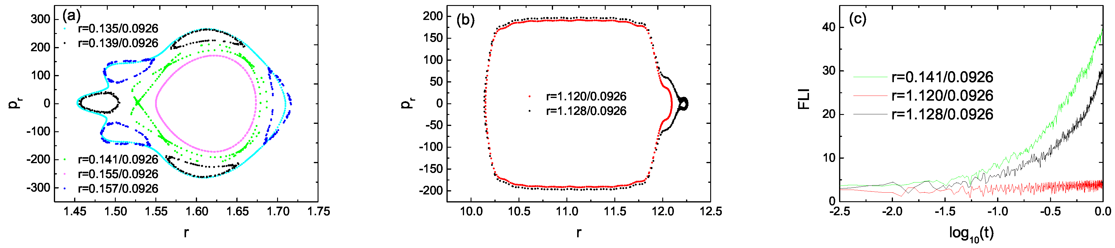
4.1. Models A4, A9 and A19

The parameters and initial conditions are those of Figure 1, but the initial values of r and $p_{\varphi }$ are different. Model A4 exhibits different phase space structures in two ranges of the initial separations r, as is shown through Poincaré sections at the plane $\varphi =\pi /2$ with $p_{\varphi }>0$ in Figure 2a,b. The three orbits in Figure 2a are KAM tori, which correspond to the regularity of the orbits. One orbit with the initial separation $r=4.430/0.1006$ and another orbit with the initial separation $r=4.424/0.1006$ in Figure 2b seem to have no explicit difference from the phase space structures on the section, but they exhibit different regular and chaotic dynamical features, which can be identified clearly by means of the technique of FLI in Figure 2c. The FLI is that with two nearby orbits defined in Ref. [35]:

$$\begin{array}{c}\hfill \mathrm{FLI}={log}_{10}\frac{d\left(t\right)}{d\left(0\right)},\end{array}$$

(22)

where $d\left(0\right)$ and $d\left(t\right)$ are the distances between two nearby orbits at time 0 and t, respectively. The orbit with the initial separation $r=4.430/0.1006$ corresponds to the FLI increasing in a power law with time ${log}_{10}t$ and is regular. However, the orbit with the initial separation $r=4.424/0.1006$ has the FLI increasing in an exponential law with time and should be chaotic. After $5\times {10}^4$ integration steps, the FLIs with completely different increasing laws with time are sensitive to distinguishing the two cases of order and chaos.

The phase space structures for Model A9 in Figure 3a are somewhat unlike those for Model A4 in Figure 2. When the initial separation r is given in a small range of $1.45<r<1.7$ for Model A4, the orbits are regular KAM tori (not plotted). However, the orbit with the initial separation $r=0.153/0.1006$ in Model A9 has several hyperbolic points. Its chaoticity is confirmed by the FLI of Figure 3c. There are no chaotic orbits in a range of $10<r<12.3$ for Model A4 in Figure 2a, but there are two chaotic orbits with the initial separations $r=1.210/0.1006$ and $r=1.235/0.1006$ in the range of $10<r<12.3$ for Model A9 in Figure 2b,c.

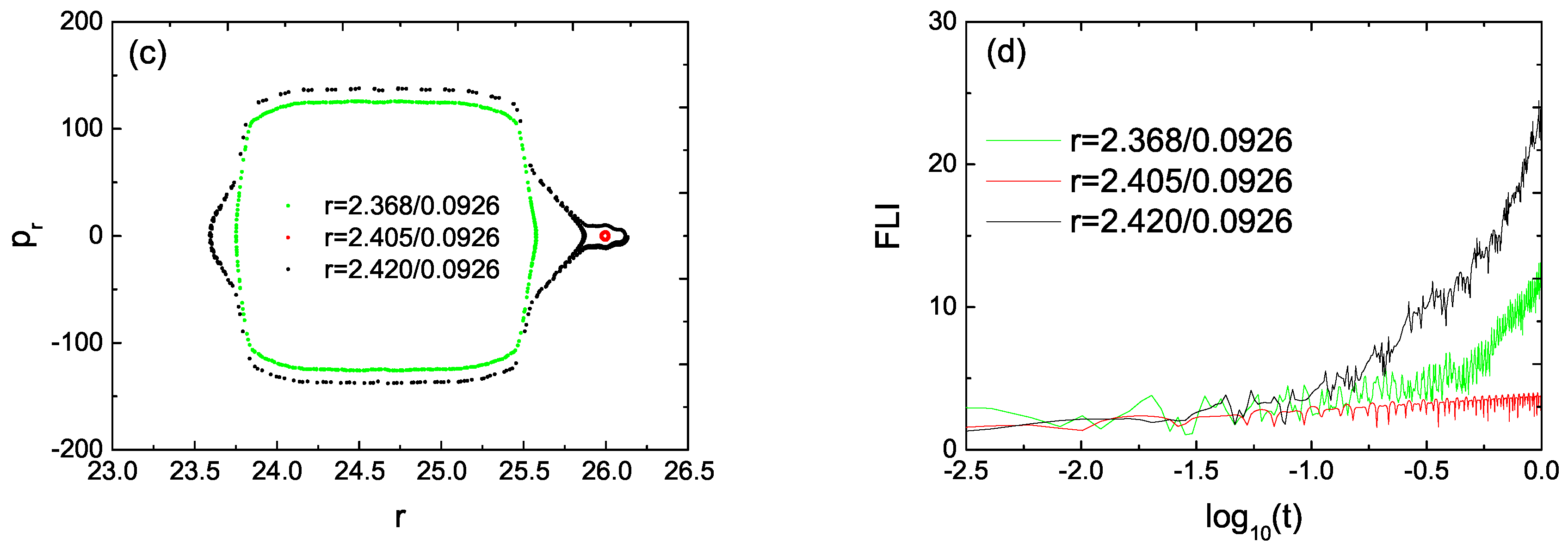
When Model A19 is considered in Figure 4a, an orbit with the initial separation $r=0.163/0.1006$ is a regular KAM torus. Another orbit with the initial separation $r=0.154/0.1006$ consists of many islands and therefore is still regular. However, the third orbit with the initial separation $r=0.160/0.1006$ is chaotic because it has many discrete points which are randomly filled with an area. The degree of chaos seems to be strengthened in the small range of $1.45<r<1.7$ from A4 to A9 and to A19. Chaos in the range of $10<r<12.5$ seems to be stronger for A19 in Figure 4b than for A9 in Figure 3b. When the initial separation r spans from 20 to 23 in Figure 2c, a lot of regular KAM torus orbits exist in the interior of the ordered orbit with the initial separation $r=2.230/0.1006$. There is a small chaotic region between the two orbits of the initial separations $r=2.230/0.1006$ and $r=2.290/0.1006$. The regularity of the orbit with the initial separation $r=2.230/0.1006$ and the chaoticity of the orbit with the initial separation $r=2.290/0.1006$ can be identified clearly by means of the technique of FLIs in Figure 4d.

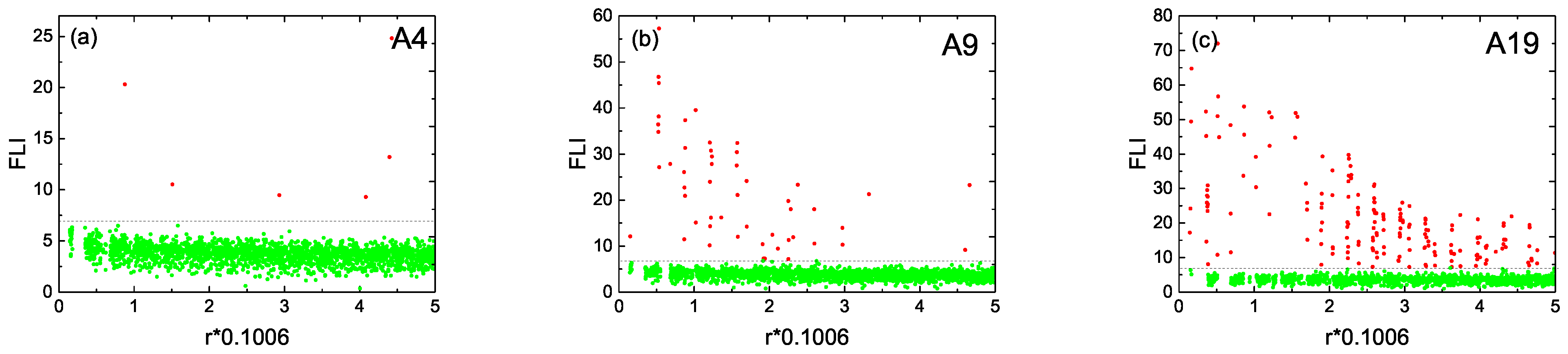
As seen from Figure 2, Figure 3 and Figure 4, the number and degree of chaotic orbits seem to increase as the number of the radial terms n becomes larger. This result is clearly shown in Figure 5, which lists the dependence of FLI on the initial separation r in Models A4, A9 and A19. In other words, Figure 5 shows that a distribution of the phase space structures of regular and chaotic orbits for each model depends on a range of the initial separation r. Each of the FLIs is obtained after $5\times {10}^4$ integration steps. Seven is a critical value of the FLI between the ordered and chaotic two cases. The FLIs not more than seven indicate the regularity of bounded orbits, whereas those larger than seven correspond to the chaoticity of the bounded orbits. The result of an increase in n increasing the number and degree of chaotic orbits is based on n corresponding to the number of the radial terms in the series expansions of the potential. An increase in n means and increases in the number of radial terms. Equivalently, the nonlinear gravitational interaction effects in the potential are enhanced.

4.2. Models B4, B9 and B19

Figure 6 describes the phase space structures of Model B4 in two ranges of the initial separations r. There is a weak chaotic orbit with the initial separation $r=0.750/0.0926$ in the range of $7.2<r<8.2$ in Figure 6a. The two orbits in the range of $10.0<r<12.2$ are regular KAM tori in Figure 6b. However, chaos occurs for the initial separation $r=3.746/0.0926$ in the range of $40.25<r<43$ in Figure 4c. The dynamical features of the chaotic orbit in panel (a) and the two orbits in panel (c) are also shown in Figure 6d. The phase space structures of Model B4 in Figure 6b,c are similar to those of Model A4 in Figure 2a,b.

The phase space structures of Model B9 in Figure 7a,b also look like those of Model A9 in Figure 3a,b. The initial separations $r=0.157/0.0926$ and $r=0.139/0.0926$ correspond to two regular orbits consisting of three loops in Figure 7a. Chaos is present for $r=0.141/0.0926$ in Figure 7a and $r=1.128/0.0926$ in Figure 7b, as the FLIs of Figure 7c show.

Model B19 seems to have stronger chaos in the ranges of $1.425<r<1.7$ and $10<r<12.25$ in Figure 8a,b than Model B9 in Figure 7a,b. For the initial separation r belonging to the range of $1.425<r<1.7$, the orbital dynamical behavior for Model B19 in Figure 8a is greatly different from that for Model A19 in Figure 4a. However, the phase space structures of Model B19 in Figure 8b,c also resemble those of Model A19 in Figure 4b,c. The FLIs of Figure 8d support the chaoticity of the two orbits for $r=2.368/0.0926$ and $r=2.420/0.0926$ in Figure 8c.

The relation between the FLI and the initial separation r in Figure 9 clearly shows that the number and degree of chaotic orbits in the B models increase with an increase in n.

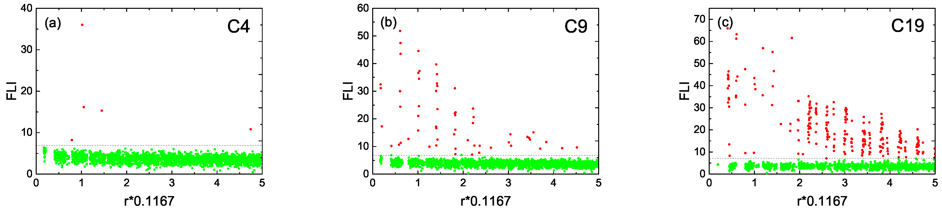
4.3. Models C4, C9 and C19

As far as the C models are concerned, chaos seems to become stronger in the range of $3.5<r<5.1$ from $n=4$ in Figure 10a to $n=9$ in Figure 10c and $n=19$ in Figure 10e. The result is also suitable for the range of $10<r<12.2$ in Figure 10b,d,f. The relation between the FLI and the initial separation r in Figure 11 supports that chaos becomes stronger with an increase in n.

Several points can be concluded from the above demonstrations. The three types of models, A, B and C, have the same expressions but have differences in the pattern speeds $\Omega$ and the coefficients $B_{i00}$, $B_{i20}$, $C_{i21}$ and $B_{i22}$. The three models have similar dynamical behaviors when they have the same radial term number n, energy E and initial conditions. The dynamical structures of ordered and chaotic orbits in each model have different distributions along the radial direction. When the radial term number n increases, the gravity effects are enhanced. This leads to strengthening the degree of chaos. It is worth noting that the main structures of the spiral arms in models A, B and C are formed at radial distances between 3 and 5 scaled radii, as is shown in Refs. [8,10]. Some ranges of the scaled radial distances, such as the range of the scaled radial distances from 40 to 43, seem to be very far from the main structures of the spiral arms. These results show that chaos can occur at the radial distances close to the main structures of the spiral arms and those far from the main structures of the spiral arms. In addition, the chaotic orbits we find are not restricted to the regions near the unstable equilibrium points $L_1$ and $L_2$. Thus, the energies selected in this paper are unlike those of [8,9,10].

5. Conclusions

This paper mainly focuses on three classes of models of rotating galaxies in the polar coordinates in the rotating frame. They are models A, B and C, which have the same expressions but have different pattern speeds $\Omega$ and different coefficients $B_{i00}$, $B_{i20}$, $C_{i21}$ and $B_{i22}$. When the potentials with large deviations from axial symmetry are included in these models, the angular momentum $p_{\varphi }$ is not a constant of motion. In this case, the kinetic energy is a function of the momenta and spatial coordinate.

The existing explicit force-gradient symplectic integrators [21,22,23,24] do not work for the present Hamiltonian problems. However, our extended force-gradient symplectic methods in the previous work [32] are still available. Numerical tests show that the fourth-order symmetric symplectic method without the extended force-gradient operator performs poorer accuracy than that with the extended force-gradient operator. In particular, the optimized extended force-gradient symplectic method is superior to the corresponding non-optimized one in accuracy.

The fourth-order-optimized symplectic algorithm with the extended force-gradient operator is applied to survey the dynamical features of regular and chaotic orbits in these rotating galaxy models. It is shown through the techniques of Poincaré sections and fast Lyapunov indicators that an increase in the radial term number of the potential strengthens the gravity effects and the degree of chaos. The three types of models have similar dynamical structures for the same radial term number, energy and initial conditions.