Article

Decision Support System Based on Complex Fractional Orthotriple Fuzzy 2-Tuple Linguistic Aggregation Operator

1
Department of Mathematics, Abdul Wali Khan University Mardan, Mardan 23200, Pakistan
2
Department of Mathematics Deanship of Applied Sciences, Umm Al-Qura University, Makkah 24231, Saudi Arabia
3
Programme of Mathematics, Faculty of Ocean Engineering Technology and Informatics, Universiti Malaysia Terengganu, Kuala Nerus 21030, Terengganu, Malaysia
4
Department of Mathematics, University of the Punjab, Lahore 54590, Pakistan
*
Author to whom correspondence should be addressed.
Symmetry 2023, 15(1), 251; https://doi.org/10.3390/sym15010251
Submission received: 17 November 2022 / Revised: 28 December 2022 / Accepted: 31 December 2022 / Published: 16 January 2023
(This article belongs to the Section Mathematics)

Abstract

:
In this research, we provide tools to overcome the information loss limitation resulting from the requirement to estimate the results in the discrete initial expression domain. Through the use of 2-tuples, which are made up of a linguistic term and a numerical value calculated between [ 0.5 , 0.5 ) , the linguistic information will be expressed. This model supports continuous representation of the linguistic data within its scope, permitting it to express any information counting received through an aggregation procedure. This study provides a novel approach to develop a linguistic multi-attribute group decision-making (MAGDM) approach with complex fractional orthotriple fuzzy 2-tuple linguistic (CFOF2TL) assessment details. Initially, the concept of a complex fractional orthotriple fuzzy 2-tuple linguistic set (CFO2TLS) is proposed to convey uncertain and fuzzy information. In the meantime, simple aggregation operators, such as CFOF2TL weighted average and geometric operators, are defined. In addition, the CFOF2TL Maclaurin’s symmetric mean (CFOF2TLMSM) operators and their weighted shapes are presented, and their attractive characteristics are also discussed. A new MAGDM approach is built using the developed aggregation operators to address managing economic crises under COVID-19 with the CFOF2TL information. As a result, the effectiveness and robustness of the developed method are accompanied by an empirical example, and a comparative study is carried out by contrasting it with previous approaches.

1. Introduction

1.1. Literature Review

Decision making (DM) is a particular behavior that combines intelligent and complex activities, taking into account vagueness and uncertainty that individuals face. The fuzzy set (FS), first proposed by Zadeh [1], is an important model in solving DM problems in an unpredictable setting. The fuzzy set has attracted much scholarly attention and research since it was published in 1965. However, one of the deficiencies of the fuzzy set is that its range is bounded to [ 0 , 1 ] , which leads to problems in communicating assessment information. For this reason, Ramot et al. [2] suggested a complex fuzzy set (CFS) by approaching the membership degree (MD) from the actual value to the complex value within the close disc. The CFS actually applies to decision theory, fuzzy logic, and other areas of science [3]. However, the fuzzy set and the CFS have a common deficiency in that they do not consider the non-membership degree (NMD) of an organization that is part of the objective in question. Then, Atanassov [4] proposed a fuzzy set expansion called an intuitionistic fuzzy set (IFS), which makes up the deficiency of the fuzzy set by adding an NMD. IFS has garnered much attention since its introduction, such as aggregation operators (AOs) [5], distance calculation [6], information entropy [7], decision method [8], and so on. Subsequently, the principle of complex IFS (CIFS), Alkouri et al. [9] identified the undetermined and uncertain specifics of a decision in practical matters. The CIFS consists of a complex MD and NMD value denoted by polar coordinates. Rani and Garg [10] specified the basic operating rules of the CIFS and proposed the MADM method for a power average and power geometric operator. Azam et al. [11] suggested a decision-making approach for the evaluation of information security management under a CIFS environment. Garg and Rani [12] defined the complex IVIFS structure and discussed its related operating rules and AOs. Garg and Rani [13] introduced a range of information measurements for information measurement theory, including similarity, entropy calculation, and so on, and further proposed a clustering algorithm based on these measures. Garg and Rani [14] proposed generalized Bonferroni mean (BM) operators using the Archimedean t-norm and Archimedean s-norm for integration of the CIF setting. Garg and Rani [15] defined some generalized CIF aggregation operators and discussed their application to MCDM. Garg and Rani [16] proposed an exponential, logarithmic generalized AOs under CIF environment. Garg and Rani [17] developed novel AOs and a ranking method for CIFSs and their applications in the DM process. However, if experts define their assessment details at ( 0.5 , 0.7 ) for MD and NMD, the IFS cannot classify it as 0.5 + 0.6 = 1.1 > 1 . Thus, Yager [18] initially offered the Pythagorean fuzzy set (PyFS) to represent the undetermined DM knowledge. It is clear that because of 0.52 + 0.72 = 0.74 < 1 , the PyFS is more general than the fuzzy set and IFS. With the PyFS in mind, Qin et al. [19] suggested some ordered weighted distance steps for DM problems. Under the Pythagorean fuzzy environment, Garg [20] described novel operational laws and proposed several aggregation operators. Liang et al. [21] joined TOPSIS methodology and three-way DM theory to develop an algorithm for DM problem solving. Khan et al. [22] extended the GRA method for the MAGDM problem under a linguistic Pythagorean fuzzy setting with incomplete weight information. Alaoui et al. [23] defined a novel analysis of fuzzy physical models by generalized fractional fuzzy operators.
Ullah et al. [24] suggested some distance measurements for the complex Pythagorean fuzzy set (CPyFS) and advanced a pattern recognition algorithm. Liu et al. [25] defined the Pythagorean fuzzy linguistic Muirhead mean operators and their applications to MADM.
Since the PyFS has a precondition that the sum of the square of MD and NMD is limited in the interval [ 0 , 1 ] , but when we come across practical situations where the knowledge given by DMs in the form of PyFS cannot fulfill the precondition, i.e., MG and NMG are given as ( 0.7 , 0.8 ) , because of 0.7 + 0.8 > 1 and 0.72 + 0.82 > 1 , the IFS and PyFS fail to communicate this effectively. On the basis of this constraint, Yager [26] established the notion of a q-rung orthopair fuzzy set (q-ROFS) to make the number of MG and NMG q-power lie in [ 0 , 1 ] . The correct q-ROFS disposes of the above example by 0.73 + 0.83 = 0.855 < 1 . It is clear that q-ROFS has generalized more than the IFS and PyFS, because the IFS and PyFS are the special cases of q-ROFS for f = 1 and f = 2 , respectively. Using this, Liu and Wang [27] developed several q-ROF Bonferroni mean operators based on the Archimedean operations. Li et al. [28] extended the idea of q-ROFS background of the EDAS method to define the DM approach. Furthermore, the concept of the Cq-ROFS and Cq-ROF linguistic set was introduced by Liu et al. [29], and many Cq-ROFL Heronian mean operators were advanced. Zhang et al. [30] developed an evaluation and selection model fora community group purchase platform based on the WEPLPA-CPT-EDAS method.
The above FSs have only represented information from a quantitative point of view, and it is difficult to give the exact numerical values for expressing their point of view on DM. Thus, Zadeh [31] developed a linguistic variable to define the qualitative setting in DM problems. After that, some new ideas, such as the single-valued neutrosophic linguistic set [32] and linguistic q-rung orthopair fuzzy sets (Lq-ROFS) [33], were proposed by joining the linguistic variable and the FS. Pei et al. [34] defined the fuzzy linguistic multi-set TOPSIS method and its application in linguistic decision making. Kong et al. [35] developed some operations on generalized hesitant fuzzy linguistic term sets. Rong et al. [36] defined hesitant fuzzy linguistic Hamy mean AOs and discussed their application to MADM. Further, Herrera and Martlnez [37] defined the idea of 2-tuple fuzzy linguistic variables and a numerical one to prevent loss of knowledge of the decision-making procedure. Some scholars [38] subsequently merged the 2-tuple linguistic variable and other FSs and developed the idea of an intuitionistic 2-tuple linguistic label (2TLL)), 2-tuple linguistic PyFSs [39], and so on. Su et al. [40] proposed the evaluation of online learning platforms based on probabilistic linguistic term sets with the self-confidence MAGDM method. Yang et al. [41] defined a decision-making structure based on Fermatean fuzzy integrated weighted distance and the TOPSIS method for green low-carbon port evaluation.
It is well-known that the aggregation operator is a key tool in the field of information fusion, and numerous research results on various aspects of it have been achieved. Xu [42] introduced several geometric AOs to aggregate intuitionistic fuzzy data. Liu and Wang [43] proposed the proven MAGDM approach to the weighted averaging and geometric operators for q-ROFS. However, these operators presume that the attributes in the integrated system are separate; i.e., they fail to take into account the interrelationships of the criteria addressed in the DM problems. To address this limitation, it is suggested that the Bonferroni mean (BM) and Heroine mean (HM) operators find the importance of the two data sources. However, the BM and the Heroine mean operator do not notice interconnections between multi-input data. Maclaurin [44] initially suggested the Maclaurin symmetric mean (MSM) operator to capture the correlation between multi-input data. Qin and Liu [45] subsequently suggested a dual MSM operator for the IF setting. Liu and Qin [46] introduced some LIMSM operators to develop an MCGDM system. Wei and Lu [47] extended the MSM operator for the Pythagorean fuzzy environment for DM problems. Liao et al. [48] proposed a q-rung orthopair fuzzy-GLDS method for investment evaluation of BE angel capital in China. Khan et al. [49] defined the linguistic interval-valued q-rung orthopair fuzzy TOPSIS method for a decision-making problem with incomplete weight.

1.2. Objective of Study

To the best of our knowledge, the MSM operator is not generalized to CFOF information. For addressing some issues, we explore the idea of complex fractional orthotriple fuzzy 2-tuple linguistic sets (CFOF2TLSs) with a condition that the sum of f-powers of the real parts of the truth, abstinence, and falsity grades does not exceed the form unit interval. So, for f = 3 , the above problem is solved effectively.
Considering the intricacy in the real circumstances and maintaining the benefits of the MSM operators and CFOF2TLSs, the goals of this research are as follows.
  • To investigate the interesting concept of CFOF2TLS and define their laws of operation
  • To define the score function, accuracy function, and comparative analysis of CFOF2TLNs.
  • To present the concept of the CFOF2TL weighted average (CFOF2TLWA) operator and CFOF2TL weighted geometric (CFOF2TLWG) operator.
  • To define several MSM operators, such as CFOF2TLMSM and CFOF2TL weighted Maclaurin symmetric mean (CFOF2TLWMSM) operators, and study the fundamental characteristics in detail.
  • To propose a MAGDM approach based on the defined aggregation operators.
  • To explain the feasibility and effectiveness of the method established by a numerical example for evaluating emergency projects.
The overall structure of the article is as follows. In Section 2, we briefly look back on some basic concepts and meanings, including the 2-tuple linguistic model, the CFOFS, and the MSM operator. In Section 3, we define the concept of CTSF2TLS, fundamental rules of operation, methodology of comparison, and fundamental operations. In Section 4, we develop the CFOF2TLA, CFOF2TLWA operator and discuss several features and their particular cases. In Section 5, we develop the CFOF2TLMSM, CFOF2TLWMSM operator and discuss several features and their particular cases. Section 6 concerns the novel MAGDM approach based on the CFOF2TLWMSM operators. In 
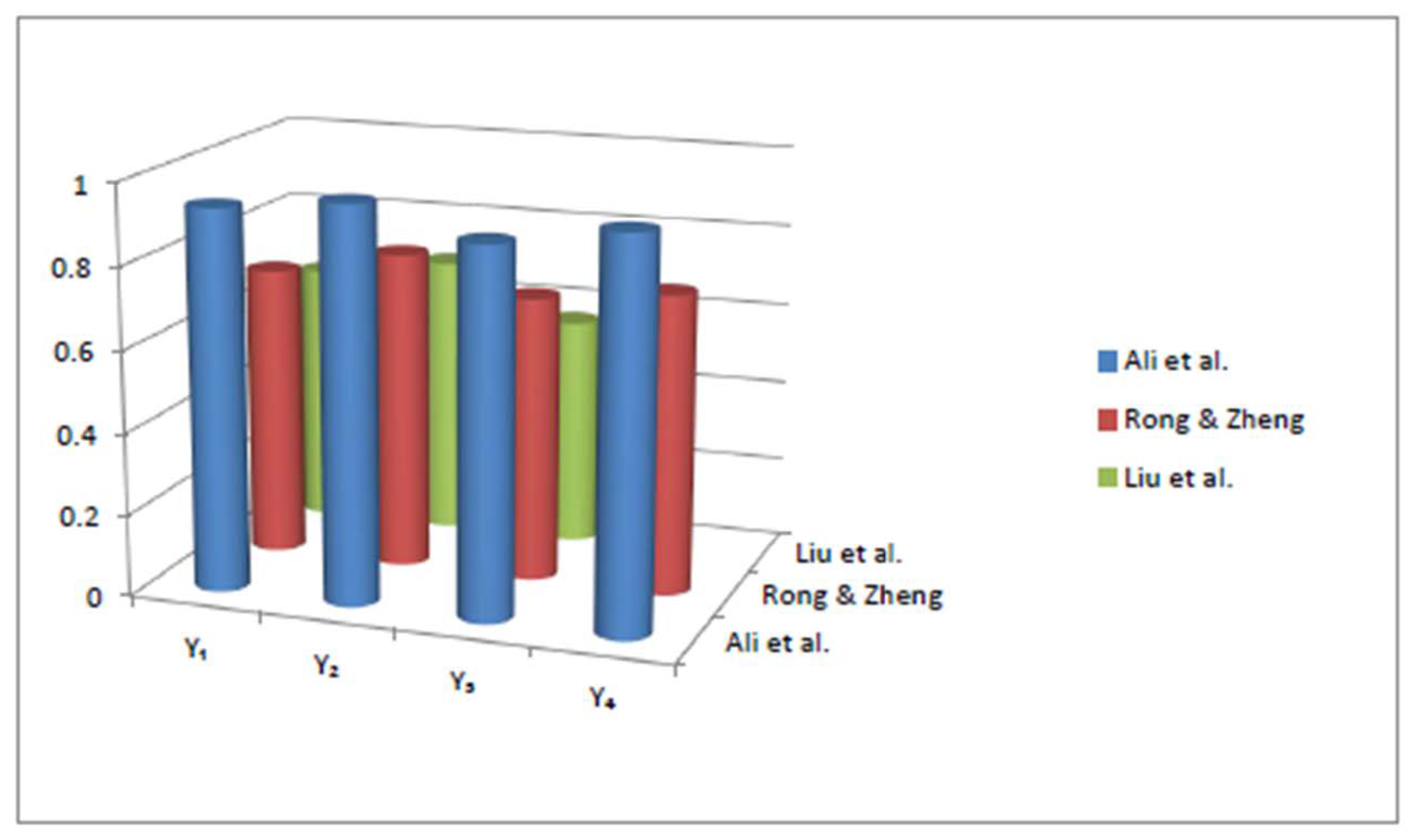
Section 7, an assessment problem of an emergency system is used to illustrate the efficiency, and a comparative study is carried out to point out the merits of the defined approach. At the end, concluding remarks are included in Section 8.

2. Preliminaries

This section concisely discusses a variety of basic information, such as the 2-tuple linguistic variable, CFOFS, and the MSM operator.

2.1. 2-Tuple Linguistic Term Set

Definition 1 
([37]). Let S = { s 0 , s 1 , , s g } be a defined linguistic term set, and the cardinality of S is g + 1 . For any s i , s j S , the following properties should be satisfied:
1. 
If i > j , then s i > s j ;
2. 
If s i s j , then max s i , s j = s i ;
3. 
If s i s j , then min s i , s j = s i ;
4. 
Neg s i = s g i .
Generally, the cardinality of the linguistic label set S is an odd number, and more than nine or less than five are both difficult for DMs to evaluate. Therefore, the cardinalities of the linguistic label set S are usually 5 , 7 , or 9 . If S is defined with five cardinalities, then it is shown as S = { s 0 = none , s 1 = very poor , s 2 = poor , s 3 = medium , s 4 = good}. In order to express linguistic information more exactly, the 2-tuple linguistic term ( s i , α ) is defined by Herrera and Martinez [37], where s i is a linguistic term involved in set S , a n d α is a numeric number denoted the deviation from s i . Some related notations of 2-tuple linguistics are provided as follows:
Definition 2 
([37]). Let S = { s 0 , s 1 , , s g } be a pre-defined linguistic term set and β [ 0 , g ] be a value denoting the result of aggregation operation. The 2-tuple linguistic ( s i , α ) is equivalent to β through the mapping Λ as follows:
Λ : [ 0 , g ] S ´ × [ 0.5 , 0.5 ) ,
Λ ( β ) = s i , i = round ( β ) α = β i , α [ 0.5 , 0.5 ) ,
where round is the usual round operation.
Obviously, Λ is a one-to-one mapping, Λ has an inverse function Λ 1 that Λ 1 : S × [ 0.5 , 0.5 ) [ 0 , g ] , and Λ 1 ( s i , α ) = α + i = β .
Definition 3. 
Let s i , α i and s j , α j be two 2-tuple linguistic terms; the relations to compare them can be given as follows:
1. 
If i > j , then s i , α i > s j , α j ;
2. 
If i = j , then
( a ) . s i , α i > s j , α j for α i > α j ;
( b ) . s i , α i < s j , α j for α i < α j ;
( c ) . s i , α i = s j , α j for α i = α j .
Definition 4 
([2]). A CFS C on universal set X is defined as C = x , σ C ( x ) | x X , where σ C : X { z : z C , z 1 } and σ C ( x ) = a 1 + i b 1 = κ C ( x ) . e 2 π i C ( x ) . Here, κ C ( x ) = a 1 2 + b 1 2 R and κ C ( x ) , C ( x ) 0 , 1 , where i = 1 .
Definition 5 
([9]). A CIFS I on universal set X is defined as I = x , σ I ( x ) , υ I ( x ) | x X , where σ I : X { z 1 : z 1 I , z 1 1 } , υ i : X { z 2 : z 2 i , z 2 1 } such that σ i ( x ) = z 1 = a 1 + i b 1 and υ i ( x ) = z 2 = a 2 + i b 2 provided that 0 z 1 + z 2 1 or σ I ( x ) = κ I ( x ) . e 2 π i κ I ( x ) and υ I ( x ) = ξ I ( x ) . e 2 π i ξ I ( x ) satisfying the conditions; 0 κ I ( x ) + ξ I ( x ) 1 and 0 κ I ( x ) + ξ I ( x ) 1 . The term H I ( x ) = R . e 2 π i R , such that R = 1 ( z 1 + z 2 ) and R ( x ) = 1 κ I ( x ) + ξ I ( x ) is called the hesitancy grade of x . Furthermore, I = κ . e 2 π i κ , ξ . e 2 π i ξ is referred to as the complex intuitionistic fuzzy number (CIFN).
Definition 6 
([50]). A CPFS P on universal set X is defined as P = { x , σ P ( x ) , η P ( x ) , υ P ( x ) | x X } , where σ P : X { z 1 : z 1 P , z 1 1 } , η P : X { z 2 : z 2 P , z 2 1 } , υ P : X { z 3 : z 3 P , z 3 1 } , such that σ P ( x ) = z 1 = a 1 + i b 1 , η P ( x ) = z 2 = a 2 + i b 2 and υ P ( x ) = z 3 = a 3 + i b 3 provided that 0 z 1 + z 2 + z 3 1 or σ P ( x ) = κ P ( x ) . e 2 π i κ P ( x ) , η P ( x ) = δ P ( x ) . e 2 π i δ P ( x ) and υ P ( x ) = ξ P ( x ) . e 2 π i ξ P ( x ) satisfying the conditions; 0 κ P ( x ) + δ P ( x ) + ξ P ( x ) 1 and 0 κ P ( x ) + δ P ( x ) + ξ P ( x ) 1 . The term H P ( x ) = R . e 2 π i R , such that R = 1 ( z 1 + z 2 + z 3 ) and R ( x ) = 1 κ P ( x ) + δ P ( x ) + ξ P ( x ) is called the hesitancy grade of x . Furthermore, P = κ . e 2 π i κ , δ . e 2 π i δ , ξ . e 2 π i ξ is referred to as a complex picture fuzzy number (CPFN).
Definition 7 
([24]). A CPyFS P on universal set X is defined as; P = { x , σ P ( x ) , υ P ( x ) | x X } , where σ P : X { z 1 : z 1 P , z 1 1 } , υ P : X { z 2 : z 2 P , z 2 1 } , such that σ P ( x ) = z 1 = a 1 + i b 1 and υ P ( x ) = z 2 = a 2 + i b 2 provided that 0 z 1 2 + z 2 2 1 or σ P ( x ) = κ P ( x ) . e 2 π i κ P ( x ) and υ P ( x ) = ξ P ( x ) . e 2 π i ξ P ( x ) satisfying the conditions; 0 κ P 2 ( x ) + ξ P 2 ( x ) 1 and 0 κ P ( x ) 2 + ξ P ( x ) 2 1 . The term H P ( x ) = R . e 2 π i R , such that R = 1 ( z 1 2 + z 2 2 ) and R ( x ) = 1 κ P ( x ) 2 + ξ P ( x ) 2 is called the hesitancy grade of X . Furthermore, P = κ . e 2 π i κ , ξ . e 2 π i ξ is referred to as complex a Pythagorean fuzzy number (CPyFN).
Definition 8 
([51]). A CSFS S on universal set X is defined as S = x , σ S ( x ) , η S ( x ) , υ S ( x ) | x X , where σ S : X { z 1 : z 1 S , z 1 1 } , η S : X { z 2 : z 2 S , z 2 1 } , υ S : X { z 3 : z 3 S , z 3 1 } , such that σ S ( x ) = z 1 = a 1 + i b 1 , η S ( x ) = z 2 = a 2 + i b 2 and υ S ( x ) = z 3 = a 3 + i b 3 provided that 0 z 1 2 + z 2 2 + z 3 2 1 or σ S ( x ) = κ S ( x ) . e 2 π i κ S ( x ) , η S ( x ) = δ S ( x ) . e 2 π i δ S ( x ) and υ S ( x ) = ξ S ( x ) . e 2 π i ξ S ( x ) satisfying the conditions; 0 κ S 2 ( x ) + δ S 2 ( x ) + ξ S 2 ( x ) 1 and 0 κ S ( x ) 2 + δ S ( x ) 2 + ξ S ( x ) 2 1 . The term H S ( x ) = R . e 2 π i R , such that R = 1 ( z 1 2 + z 2 2 + z 3 2 ) and R ( x ) = 1 κ S ( x ) 2 + δ S ( x ) 2 + ξ S ( x ) 2 are called the hesitancy grade of X . Furthermore, S = κ . e 2 π i κ , δ . e 2 π i δ , ξ . e 2 π i ξ is referred to as a complex spherical fuzzy number (CSFN).
Definition 9. 
A CFOFS ϝ on universal set X is defined as ϝ = { x , σ ϝ ( x ) , η ϝ ( x ) , υ ϝ ( x ) | x X } , where σ ϝ : X { z 1 : z 1 ϝ , z 1 1 } , η ϝ : X { z 2 : z 2 ϝ , z 2 1 } , υ ϝ : X { z 3 : z 3 ϝ , z 3 1 } , such that σ ϝ ( x ) = z 1 = a 1 + i b 1 , η ϝ ( x ) = z 2 = a 2 + i b 2 and υ ϝ ( x ) = z 3 = a 3 + i b 3 provided that 0 z 1 f + z 2 f + z 3 f 1 or σ ϝ ( x ) = κ ϝ ( x ) . e 2 π i κ ϝ ( x ) , η ϝ ( x ) = δ ϝ ( x ) . e 2 π i δ ϝ ( x ) and υ ϝ ( x ) = ξ ϝ ( x ) . e 2 π i ξ ϝ ( x ) satisfy the conditions: 0 κ ϝ f ( x ) + δ ϝ f ( x ) + ξ ϝ f ( x ) 1 and 0 κ ϝ ( x ) f + δ ϝ ( x ) f + ξ ϝ ( x ) f 1 . The term H ϝ ( x ) = R . e 2 π i R , such that R = 1 ( z 1 f + z 2 f + z 3 f ) f and R ( x ) = 1 κ ϝ ( x ) f + δ ϝ ( x ) f + ξ ϝ ( x ) f f are called the hesitancy grade of X . Furthermore, ϝ = κ . e 2 π i κ , δ . e 2 π i δ , ξ . e 2 π i ξ is referred as a complex fractional orthotriple fuzzy number (CFOFN).
Definition 10. 
Let ϝ 1 = κ 1 ( x ) e 2 π i κ 1 ( x ) , δ 1 ( x ) e 2 π i δ 1 ( x ) , ξ 1 ( x ) e 2 π i ξ 1 ( x ) and ϝ 2 = κ 2 ( x ) e 2 π i κ 2 ( x ) , δ 2 ( x ) e 2 π i δ 2 ( x ) , ξ 2 ( x ) e 2 π i ξ 2 ( x ) be the two CFOFNs with λ 0 . Then, the operational laws are described as:
  • ϝ 1 ϝ 2 = κ 1 f ( x ) + κ 2 f ( x ) κ 1 f ( x ) κ 2 f ( x ) 1 f e 2 π i κ 1 ( x ) f + κ 2 ( x ) f κ 1 ( x ) f κ 2 ( x ) f 1 f , δ 1 ( x ) . δ 2 ( x ) e 2 π i δ 1 ( x ) δ 2 ( x ) , ξ 1 ( x ) ξ 2 ( x ) e 2 π i ξ 1 ( x ) ξ 2 ( x ) ;
  • ϝ 1 ϝ 2 = κ 1 ( x ) κ 2 ( x ) e 2 π i κ 1 ( x ) κ 2 ( x ) , δ 1 f ( x ) + δ 2 f ( x ) δ 1 f ( x ) δ 2 f ( x ) 1 f e 2 π i δ 1 ( x ) f + δ 2 ( x ) f δ 1 ( x ) f δ 2 ( x ) f 1 f , v 1 f ( x ) + ξ 2 f ( x ) ξ 1 f ( x ) ξ 2 f ( x ) 1 f e 2 π i ξ 1 ( x ) f + ξ 2 ( x ) f ξ 1 ( x ) f ξ 2 ( x ) f 1 f ;
  • λ ϝ 1 = 1 1 κ 1 f ( x ) λ 1 f e 2 π i 1 1 κ 1 ( x ) f λ 1 f , δ 1 λ ( x ) e 2 π i δ ϝ 1 ( x ) λ , ξ 1 λ ( x ) e 2 π i ξ 1 ( x ) λ ;
  • ϝ 1 λ = κ 1 λ ( x ) e 2 π i κ 1 ( x ) λ , 1 1 δ 1 f ( x ) λ 1 f e 2 π i 1 1 δ 1 ( x ) f λ 1 f , 1 1 ξ 1 f ( x ) λ 1 f e 2 π i 1 1 ξ 1 ( x ) f λ 1 f ;
Definition 11. 
Let ϝ 1 = κ 1 ( x ) e 2 π i κ 1 ( x ) , δ 1 ( x ) e 2 π i δ 1 ( x ) , ξ 1 ( x ) e 2 π i ξ 1 ( x ) be a CFOFN. Then, the score and accuracy functions are defined as:
S c * ϝ 1 = κ f δ f ξ f + κ f δ f ξ f ,
and
H c * ϝ 1 = κ f + δ f + ξ f + κ f + δ f + ξ f ,
where S c * ϝ 1 [ 2 , 2 ] , and H c * ϝ 1 [ 0 , 2 ] .
Definition 12. 
The following comparison rules between two CFOFNs ϝ 1 and ϝ 2 are satisfied:
1. 
If S c * ϝ 1 > S c * ϝ 2 , then ϝ 1 > ϝ 2 ;
2. 
If S c * ϝ 1 = S c * ϝ 2 , then
(a). If H c * ϝ 1 > H c * ϝ 2 , then ϝ 1 > ϝ 2 ;
(b). If H c * ϝ 1 = H c * ϝ 2 , then ϝ 1 = ϝ 2 .

2.2. Maclaurin Symmetric Mean (MSM) Operator

Definition 13 
([44]). The MSM operator is mathematically defined as follows:
M S M ( k ) ( e 1 , , e n ) = 1 r 1 < . . . < r k n j = 1 k e r j C n k 1 k ,
where k represents a parameter of r 1 , , r k ( k = 1 , , n ) , and the values k integer is obtained from the set of ( 1 , , n ) of n integer values. C n k represents the binomial coefficient, and C n k = n ! k ! n k ! .
The below properties must be satisfied by the MSM operator:
  • M S M ( k ) 0 , , 0 = 0 ;
  • M S M ( k ) ( e 1 , , e n ) = e , if e i = e , ( i = 1 , , n ) ;
  • M S M ( k ) ( e 1 , , e n ) M S M ( k ) ( e ˜ 1 , , e ˜ n ) , if e i e ˜ i , for all i ;
  • min i { e i } M S M ( k ) ( e 1 , , e n ) max i { e i } .

3. Complex Fractional Orthotriple Fuzzy 2-Tuple Linguistic Set

Basic definitions, score, accuracy functions, and some operators on CFOF2TLS are defined in this section.
Definition 14. 
Let X be a fixed set. Then, the CFOF2TLS is expressed as:
ϝ 1 = s θ 1 ( x ) , 1 , σ 1 ( x ) , η 1 ( x ) , υ 1 ( x ) | x X ,
where s θ ( x ) S , [ 0.5 , 0.5 ) , σ 1 ( x ) = κ 1 ( x ) . e 2 π i κ 1 ( x ) , η 1 ( x ) = δ 1 ( x ) . e 2 π i δ 1 ( x ) and υ 1 ( x ) = ξ 1 ( x ) . e 2 π i ξ 1 ( x ) indicate complex-valued positive, neutral, and negative grade of the element x belongs to the linguistic variable s θ ( x ) , , correspondingly. Also satisfy the characteristic 0 σ 1 f ( x ) , η 1 f ( x ) , υ 1 f ( x ) 1 and 0 κ S ( x ) f + δ S ( x ) f + ξ S ( x ) f 1 . The term H ϝ ( x ) = R . e 2 π i R , such that R = 1 ( z 1 f + z 2 f + z 3 f ) f and R ( x ) = 1 κ ϝ ( x ) f + δ ϝ ( x ) f + ξ ϝ ( x ) f f is considered as a hesitancy grade of X. Furthermore,
ϝ = s θ ( x ) , κ . e 2 π i κ , δ . e 2 π i δ , ξ . e 2 π i ξ is referred to as a complex fractional orthotriple fuzzy 2-tuple linguistic number (CFOF2TLN).
Definition 15. 
Let ϝ 1 = s θ 1 ( x ) , 1 κ 1 ( x ) e 2 π i κ 1 ( x ) , δ 1 ( x ) e 2 π i δ ϝ 1 ( x ) , ξ 1 ( x ) e 2 π i ξ 1 ( x ) be a CFOF2TLN. Then, the score index and accuracy index are defined as:
S c * ϝ 1 = κ 1 f δ 1 f ξ 1 f + κ 1 f δ 1 f ξ 1 f Λ 1 s θ 1 ( x ) , 1 ,
and
H c * ϝ 1 = κ 1 f + δ 1 f + ξ 1 f + κ 1 f + δ 1 f + ξ 1 f Λ 1 s θ 1 ( x ) , 1 .
Definition 16. 
The following comparison rules between two CFOF2TLNs ϝ 1 and ϝ 2 are satisfied:
1. 
If S c * ϝ 1 > S c * ϝ 2 , then ϝ 1 > ϝ 2 ;
2. 
If S c * ϝ 1 = S c * ϝ 2 , then
(a). If H c * ϝ 1 > H c * ϝ 2 , then ϝ 1 > ϝ 2 ;
(b). If H c * ϝ 1 = H c * ϝ 2 , then ϝ 1 = ϝ 2 .
Definition 17. 
Let ϝ 1 = s θ 1 ( x ) , 1 κ 1 ( x ) e 2 π i κ 1 ( x ) , δ 1 ( x ) e 2 π i δ 1 ( x ) , ξ 1 ( x ) e 2 π i ξ 1 ( x ) and ϝ 2 = s θ 2 ( x ) , 2 κ 2 ( x ) e 2 π i κ 2 ( x ) , δ 2 ( x ) e 2 π i δ 2 ( x ) , ξ 2 ( x ) e 2 π i ξ 2 ( x ) be the CFOF2TLNs with λ 0 . Then, the operation laws are defined as:
1. 
ϝ 1 ϝ 2 = Λ Λ 1 s θ 1 ( x ) , 1 + s θ 2 ( x ) , 2 , κ 1 f ( x ) + κ 2 f ( x ) κ 1 f ( x ) κ 2 f ( x ) 1 f e 2 π i κ 1 ( x ) f + κ 2 ( x ) f κ 1 ( x ) f κ 2 ( x ) f 1 f , δ 1 ( x ) . δ 2 ( x ) e 2 π i δ 1 ( x ) δ 2 ( x ) , ξ 1 ( x ) ξ 2 ( x ) e 2 π i ξ 1 ( x ) ξ 2 ( x ) ;
2. 
ϝ 1 ϝ 2 = Λ Λ 1 s θ 1 ( x ) , 1 × s θ 2 ( x ) , 2 , κ ϝ 1 ( x ) κ 2 ( x ) . e 2 π i κ ϝ 1 ( x ) κ 2 ( x ) , δ 1 f ( x ) + δ 2 f ( x ) δ ϝ 1 f ( x ) δ 2 f ( x ) 1 f e 2 π i δ 1 ( x ) f + δ 2 ( x ) f δ ϝ 1 ( x ) f δ 2 ( x ) f 1 f , v ϝ 1 f ( x ) + ξ 2 f ( x ) ξ ϝ 1 f ( x ) ξ 2 f ( x ) 1 f e 2 π i ξ 1 ( x ) f + ξ 2 ( x ) f ξ 1 ( x ) f ξ 2 ( x ) f 1 f ;
3. 
λ ϝ 1 = Λ λ Λ 1 s θ 1 ( x ) , 1 , 1 1 κ 1 f ( x ) λ 1 f e 2 π i 1 1 κ 1 ( x ) f λ 1 f , δ 1 λ ( x ) e 2 π i δ ϝ 1 ( x ) λ , ξ 1 λ ( x ) e 2 π i ξ 1 ( x ) λ ;
4. 
ϝ 1 λ = Λ Λ 1 s θ 1 ( x ) , 1 λ , κ 1 λ ( x ) e 2 π i κ 1 ( x ) λ , 1 1 δ 1 f ( x ) λ 1 f e 2 π i 1 1 δ ϝ 1 ( x ) f λ 1 f , 1 1 ξ 1 f ( x ) λ 1 f e 2 π i 1 1 ξ 1 ( x ) f λ 1 f .

4. Aggregation Operators on Complex Fractional Orthotriple Fuzzy 2-Tuple Linguistic Numbers

Definition 18. 
Let ϝ i = s θ i ( x ) , i κ i ( x ) e 2 π i κ i ( x ) , δ i ( x ) e 2 π i δ i ( x ) , ξ i ( x ) e 2 π i ξ i ( x ) ( i = 1 , , n ) be a family of CFOF2TLNs. A function Φ n Φ is said to be CFOF2TLWA operator and is defined as:
C F O F 2 T L W A ( ϝ 1 , , ϝ n ) = i = 1 n w i ϝ i ,
where Φ represents the family of CFOF2TLNs, w i is the weight vector, such that w i [ 0 , 1 ] and i = 1 n w i = 1 .
Theorem 1. 
Let ϝ i = s θ i ( x ) , i κ i ( x ) e 2 π i κ i ( x ) , δ i ( x ) e 2 π i δ i ( x ) , ξ i ( x ) e 2 π i ξ i ( x ) ( i = 1 , , n ) be a family of CFOF2TLNs, and w i be the weight, such that w i [ 0 , 1 ] and i = 1 n w i = 1 . Then, the result obtained from the CFOF2TLWA operator is still a CFOF2TLN, and‘
C F O F 2 T L W A ( ϝ 1 , , ϝ n ) = Λ i = 1 n w i Λ 1 s θ i ( x ) , i , 1 i = 1 n 1 κ i f ( x ) w i 1 f e 2 π i 1 i = 1 n 1 κ i ( x ) f w i 1 f , i = 1 n δ i w i ( x ) e 2 π i i = 1 n δ i ( x ) w i , i = 1 n ξ i w i ( x ) e 2 π i i = 1 n ξ i ( x ) w i .
Theorem 2. 
Let ϝ i = s θ i ( x ) , i κ i ( x ) e 2 π i κ i ( x ) , δ i ( x ) e 2 π i δ i ( x ) , ξ i ( x ) e 2 π i ξ i ( x ) ( i = 1 , , n ) be a family of CFOF2TLNs. Then, the CFOF2TLWA operator has the below properties:
1. 
(Idempotency). If all CFOF2TLNs are equal, i.e., ϝ i = ϝ for all i , then
C F O F 2 T L W A ( ϝ 1 , , ϝ n ) = ϝ .
2. 
(Monotonicity). For ϝ i and ϝ ˜ i ( i = 1 , , n ) , if ϝ i ϝ ˜ i , for all i . Then,
C F O F 2 T L W A ( ϝ 1 , , ϝ n ) C F O F 2 T L W A ( ϝ ˜ 1 , , ϝ ˜ n ) .
3. 
(Boundedness). Let ϝ i ( i = 1 , , n ) be a family of CFOF2TLNs, and ϝ i = min i { ϝ i } , ϝ i + = max i { ϝ i } . Then,
ϝ i C F O F 2 T L W A ( ϝ 1 , , ϝ n ) ϝ i + .
Definition 19. 
Let ϝ i = s θ i ( x ) , i κ i ( x ) e 2 π i κ i ( x ) , δ i ( x ) e 2 π i δ i ( x ) , ξ i ( x ) e 2 π i ξ i ( x ) ( i = 1 , , n ) be a family of CFOF2TLNs. A function Φ n Φ is said to be a CFOF2TLWG operator and defined as:
C F O F 2 T L W G ( ϝ 1 , , ϝ n ) = i = 1 n ϝ i w i ,
where Φ represent the family of CFOF2TLNs, w i are the weights, such that w i [ 0 , 1 ] and i = 1 n w i = 1 .
Theorem 3. 
Let ϝ i = s θ i ( x ) , i κ i ( x ) e 2 π i κ i ( x ) , δ i ( x ) e 2 π i δ i ( x ) , ξ i ( x ) e 2 π i ξ i ( x ) ( i = 1 , , n ) be a family of CFOF2TLNs, and w i are the weights, such that w i [ 0 , 1 ] and i = 1 n w i = 1 . Then, the value obtained from the CFOF2TLWG operator is still a CFOF2TLNs, and
C F O F 2 T L W G ( ϝ 1 , , ϝ n ) = Λ i = 1 n Λ 1 s θ i ( x ) , i w i , i = 1 n κ i w i ( x ) e 2 π i i = 1 n κ i ( x ) w i , 1 i = 1 n 1 δ i f ( x ) w i 1 f e 2 π i 1 i = 1 n 1 δ i ( x ) f w i 1 f , 1 i = 1 n 1 ξ i f ( x ) w i 1 f e 2 π i 1 i = 1 n 1 ξ i ( x ) f w i 1 f .
Theorem 4. 
Let ϝ i = s θ i ( x ) , i κ ϝ i ( x ) e 2 π i κ ϝ i ( x ) , δ ϝ i ( x ) e 2 π i δ ϝ i ( x ) , ξ ϝ i ( x ) e 2 π i ξ ϝ i ( x ) ( i = 1 , , n ) be a family of CFOF2TLNs. Then, the CFOF2TLWG operator possesses the following features:
1. 
(Idempotency). If all CFOF2TLNs are equal, i.e., ϝ i = ϝ for all i , then
C F O F 2 T L W G ( ϝ 1 , , ϝ n ) = ϝ .
2. 
(Monotonicity). For ϝ i and ϝ ˜ i ( i = 1 , , n ) , if ϝ i ϝ ˜ i , for all i . Then,
C F O F 2 T L W G ( ϝ 1 , , ϝ n ) C F O F 2 T L W G ( ϝ ˜ 1 , , ϝ ˜ n ) .
3. 
(Boundedness). Let ϝ i ( i = 1 , , n ) be the family of CFOF2TLNs, and ϝ i = min i { ϝ i } , ϝ i + = max i { ϝ i } . Then,
ϝ i C F O F 2 T L W G ( ϝ 1 , , ϝ n ) ϝ i + .

5. The Complex Fractional Orthotriple Fuzzy 2-Tuple Linguistic Maclaurin’s Symmetric Mean Operators

In this portion, we generalize the MSM operator to the proposed CFOF2TL environment to build up the CFOF2TLMSM operator. Further, we define their weighted CFOF2TLWMSM operator.

5.1. The CFOF2TLMSM Operator

Definition 20. 
Let ϝ i = s θ i ( x ) , i κ i ( x ) e 2 π i κ i ( x ) , δ i ( x ) e 2 π i δ i ( x ) , ξ i ( x ) e 2 π i ξ i ( x ) ( i = 1 , , n ) be a family of CFOF2TLNs. A function Φ n Φ known as a CFOF2TLMSM operator is:
C F O F 2 T L M S M ( k ) ( ϝ 1 , , ϝ n ) = 1 r 1 < . . . < r k n i = 1 k ϝ r i C n k 1 k ,
where Φ stands for the family of CFOF2TLNs, k 1 , , n is a parameter, r 1 , , r k are the k integer values obtained from the family ( 1 , , n ) of the n integer values, C n k represents the binomial coefficient, and C n k = n ! k ! n k ! .
Theorem 5. 
Let ϝ i = s θ i ( x ) , i κ i ( x ) e 2 π i κ i ( x ) , δ i ( x ) e 2 π i δ i ( x ) , ξ i ( x ) e 2 π i ξ i ( x ) ( i = 1 , , n ) be a family of CFOF2TLNs, the result of ( ϝ 1 , , ϝ n ) is obtained by utilizing the CFOF2TLMSM operator described as:
C F O F 2 T L M S M ( k ) ( ϝ 1 , . . . , ϝ n ) = Λ ψ i = 1 n Λ 1 s θ r i ( x ) , r i C n k 1 k , 1 ψ 1 i = 1 k κ r i ( x ) f 1 C n k 1 f 1 k e 2 π i 1 ψ 1 i = 1 k κ r i ( x ) f 1 C n k 1 f 1 k , 1 1 ψ 1 i = 1 k 1 δ r i ( x ) f 1 C n k 1 k 1 f e 2 π i 1 1 ψ 1 i = 1 k 1 δ r i ( x ) f 1 C n k 1 k 1 f 1 1 ψ 1 i = 1 k 1 ξ r i ( x ) f 1 C n k 1 k 1 f e 2 π i 1 1 ψ 1 i = 1 k 1 ξ r i ( x ) f 1 C n k 1 k 1 f ,
where ψ represents the subscript ( 1 r 1 < < r k n ) .
Proof. 
For proof, see Appendix A. □
Theorem 6. 
(Idempotency). Let ϝ i = { s θ i ( x ) , i , κ i ( x ) e 2 π i κ i ( x ) , δ ϝ i ( x ) e 2 π i δ i ( x ) , ξ i ( x ) e 2 π i ξ i ( x ) } ( i = 1 , , n ) be a family of CFOF2TLNs. If all CFOF2TLNs are equal, i.e., ϝ i = ϝ , i , then
C F O F 2 T L M S M ( ϝ 1 , , ϝ n ) = ϝ .
Proof. 
For proof, see Appendix B. □
Theorem 7. 
(Monotonicity). Let ϝ i = { s θ i ( x ) , i , κ i ( x ) e 2 π i κ i ( x ) , δ ϝ i ( x ) e 2 π i δ i ( x ) , ξ i ( x ) e 2 π i ξ i ( x ) } ( i = 1 , , n ) be a family of CFOF2TLNs. iIf ϝ i ϝ ˜ i , for all i , then
C F O F 2 T L M S M ( ϝ 1 , , ϝ n ) C F O F 2 T L M S M ( ϝ ˜ 1 , , ϝ ˜ n ) .
Proof. 
For proof, see Appendix C. □
Theorem 8. 
(Boundedness). Let ϝ i = { s θ i ( x ) , i , κ i ( x ) e 2 π i κ i ( x ) , δ ϝ i ( x ) e 2 π i δ i ( x ) , ξ i ( x ) e 2 π i ξ i ( x ) } ( i = 1 , , n ) be a family of CFOF2TLNs, and ϝ i = min i { ϝ i } , ϝ i + = max i { ϝ i } . Then,
ϝ i C F O F 2 T L M S M ( ϝ 1 , , ϝ n ) ϝ i + .
Proof. 
For proof, see Appendix D. □
A number of novel operators will be calculated in the next step by assigning various values of k .
  • If k = 1 , the CFOF2TLMSM operator is reduced to a CFOF2TL arithmetic average (CFOF2TLAA) operator, defined as follows:
    C F O F 2 T L M S M ( 1 ) ( ϝ 1 , . . . , ϝ n ) = 1 n 1 r 1 n ϝ r i = 1 n r = 1 n ϝ r let r 1 = r = Λ 1 n r = 1 n Λ 1 s θ r ( x ) , r , 1 r = 1 n 1 κ r f ( x ) 1 n 1 f e 2 π i 1 r = 1 n 1 ξ r ( x ) f 1 n 1 f , r = 1 n δ ϝ r 1 n ( x ) e 2 π i r = 1 n δ r ( x ) 1 n , r = 1 n ξ r 1 n ( x ) e 2 π i r = 1 n ξ r ( x ) 1 n .
  • If k = 2 , the CFOF2TLMSM operator is reduced to a CFOF2TL Bonferroni mean (CFOF2TLBM) operator, defined as follows:
    C F O F 2 T L M S M ( 2 ) ( ϝ 1 , . . . , ϝ n ) = 1 r 1 < r 2 n i = 1 2 ϝ r i C n 3 1 2 = 1 n ( n 1 ) r 1 , r 2 = 1 r 1 r 2 k ϝ r 1 1 ϝ r 2 1 1 2 = Λ 1 n ( n 1 ) r 1 , r 2 = 1 r 1 r 2 k Λ 1 s θ r 1 ( x ) , r 1 Λ 1 s θ r 1 ( x ) , r 1 1 2 , 1 r 1 , r 2 = 1 r 1 r 2 k 1 κ ϝ r 1 f ( x ) κ r 2 f ( x ) 2 n ( n 1 ) 1 f 1 2 e 2 π i 1 r 1 , r 2 = 1 r 1 r 2 k 1 ξ r 1 ( x ) f ξ r 2 ( x ) f 1 n ( n 1 ) 1 f 1 2 , 1 1 r 1 , r 2 = 1 r 1 r 2 k 1 1 δ r 1 f ( x ) 1 δ r 2 f ( x ) 1 n ( n 1 ) 1 2 1 f e 2 π i 1 1 r 1 , r 2 = 1 r 1 r 2 n 1 1 δ r 1 ( x ) f 1 δ r 2 ( x ) f 1 n ( n 1 ) 1 2 1 f 1 1 r 1 , r 2 = 1 r 1 r 2 n 1 1 ξ r 1 f ( x ) 1 ξ r 2 f ( x ) 1 n ( n 1 ) 1 2 1 f e 2 π i 1 1 r 1 , r 2 = 1 r 1 r 2 n 1 1 ξ r 1 ( x ) f 1 ξ r 2 ( x ) f 1 n ( n 1 ) 1 2 1 f .
  • If k = 3 , the CFOF2TLMSM operator becomes a CFOF2TL generalized Bonferroni mean (CFOF2TLGBM) operator, defined as follows:
    C F O F 2 T L M S M ( 3 ) ( ϝ 1 , . . . , ϝ n ) = 1 r 1 < r 2 n i = 1 3 ϝ r i C n 3 1 3 = 1 n ( n 1 ) ( n 2 ) r 1 , r 2 , r 3 = 1 r i r j r p k ϝ r 1 1 ϝ r 2 1 ϝ r 3 1 1 3 .
  • If k = n , the CFOF2TLMSM operator is reduced to a CFOF2TL geometric mean (CFOF2TLGM) operator, defined as follows:
    C F O F 2 T L M S M ( n ) ( ϝ 1 , . . . , ϝ n ) = 1 n i = 1 n ϝ r 1 n = Λ r = 1 n Λ 1 s θ r ( x ) , r 1 n , r = 1 n κ r ( x ) 1 n e 2 π i r = 1 n ξ r ( x ) f 1 n , 1 r = 1 n 1 δ r f ( x ) 1 n 1 f e 2 π i 1 r = 1 n 1 δ r ( x ) f 1 n 1 f , 1 r = 1 n 1 ξ r f ( x ) 1 n 1 f e 2 π i 1 r = 1 n 1 ξ r ( x ) f 1 n 1 f .

5.2. The CFOF2TLWMSM Operator

The attribute weight is an important predictor in practical decision problems. We propose the CFOF2TLWMSM operators compensate for the defectiveness of the operator of CFOF2TLMSM as follows:
Definition 21. 
Let ϝ i = s θ i ( x ) , i κ i ( x ) e 2 π i κ i ( x ) , δ i ( x ) e 2 π i δ i ( x ) , ξ i ( x ) e 2 π i ξ i ( x ) ( i = 1 , , n ) be a family of CFOF2TLNs and w i be the weights of ϝ i , where w i [ 0 , 1 ] and i = 1 n w i = 1 . A function Φ n Φ known as a CFOF2TLMSM operator defined as:
C F O F 2 T L W M S M ( k ) ( ϝ 1 , , ϝ n ) = 1 r 1 < . . . < r k n i = 1 k ϝ r i w i C n k 1 k ,
where Φ stands for the family of CFOF2TLNs, k is a parameter and k ( 1 , , n ) , r 1 , , r k are the k integer values obtained from the family ( 1 , , n ) of the n integer values, C n k represents the binomial coefficient, and C n k = n ! k ! n k ! .
Theorem 9. 
Let ϝ i = s θ i ( x ) , i κ i ( x ) e 2 π i κ i ( x ) , δ i ( x ) e 2 π i δ i ( x ) , ξ i ( x ) e 2 π i ξ i ( x ) ( i = 1 , , n ) be a family of CFOF2TLNs, the result of ( ϝ 1 , , ϝ n ) is obtained by using a CFOF2TLWMSM operator expressed as:
C F O F 2 T L W M S M ( k ) ( ϝ 1 , . . . , ϝ n ) = Λ ψ i = 1 k Λ 1 s θ r i ( x ) , r i w r i C n k 1 k , 1 ψ 1 i = 1 k κ r i ( x ) w r i f 1 C n k 1 f 1 k e 2 π i 1 ψ 1 i = 1 k κ r i ( x ) w r i f 1 C n k 1 f 1 k , 1 1 ψ 1 i = 1 k 1 δ r i ( x ) f w r i 1 C n k 1 k 1 f e 2 π i 1 1 ψ 1 i = 1 k 1 δ r i ( x ) f w r i 1 C n k 1 k 1 f 1 1 ψ 1 i = 1 k 1 ξ r i ( x ) f w r i 1 C n k 1 k 1 f e 2 π i 1 1 ψ 1 i = 1 k 1 ξ r i ( x ) f w r i 1 C n k 1 k 1 f ,
where ψ represents the subscript ( 1 r 1 < < r k n ) .
Proof. 
For proof, see Appendix E. □
A number of novel operators will be calculated in the next step by assigning various values of k .
  • If k = 1 , the CFOF2TLWMSM operator is reduced to a CFOF2TL weighted average (CFOF2TLWA) operator, defined as follows:
    C F O F 2 T L W M S M ( 1 ) ( ϝ 1 , . . . , ϝ n ) = 1 n 1 r 1 n ϝ r i w r i = 1 n r = 1 n ϝ r w r i = Λ 1 n r = 1 n Λ 1 s θ r ( x ) , r w r i , 1 r = 1 n 1 κ r f ( x ) w r i 1 n 1 f e 2 π i 1 r = 1 n 1 ξ r ( x ) f w r i 1 n 1 f , r = 1 n δ ϝ r f ( x ) e 2 π i r = 1 n δ r ( x ) 1 n , r = 1 n ξ r f ( x ) e 2 π i r = 1 n ξ r ( x ) 1 n .
  • If k = 2 , the CFOF2TLWMSM operator is reduced to a CFOF2TL weighted Bonferroni mean (CFOF2TLWBM) operator, defined as follows:
    C F O F 2 T L W M S M ( 2 ) ( ϝ 1 , . . . , ϝ n ) = 1 r 1 < r 2 n i = 1 2 ϝ r i w r i C n 2 1 2 = 1 n ( n 1 ) r 1 , r 2 = 1 r 1 r 2 k ϝ r 1 w r 1 ϝ r 2 w r 2 1 2 = Λ 1 n ( n 1 ) r 1 , r 2 = 1 r 1 r 2 k Λ 1 s θ r 1 ( x ) , r 1 w r 1 Λ 1 s θ r 1 ( x ) , r 1 w r 2 1 2 , 1 r 1 , r 2 = 1 r 1 r 2 k 1 κ ϝ r 1 ( x ) w r 1 κ r 2 ( x ) w r 2 f 2 n ( n 1 ) 1 f 1 2 e 2 π i 1 r 1 , r 2 = 1 r 1 r 2 k 1 ξ r 1 ( x ) w r 1 ξ r 2 ( x ) f w r 1 1 n ( n 1 ) 1 f 1 2 , 1 1 r 1 , r 2 = 1 r 1 r 2 k 1 1 δ r 1 f ( x ) 1 δ r 2 f ( x ) 1 n ( n 1 ) 1 2 1 f e 2 π i 1 1 r 1 , r 2 = 1 r 1 r 2 n 1 1 δ r 1 ( x ) f w r 1 1 δ r 2 ( x ) f w r 2 f 1 n ( n 1 ) 1 2 1 f 1 1 r 1 , r 2 = 1 r 1 r 2 n 1 1 ξ r 1 f ( x ) w r 1 1 ξ r 2 f ( x ) w r 2 1 n ( n 1 ) 1 2 1 f e 2 π i 1 1 r 1 , r 2 = 1 r 1 r 2 n 1 1 ξ r 1 ( x ) f w r 1 1 ξ r 2 ( x ) f w r 2 1 n ( n 1 ) 1 2 1 f .
  • If k = 3 , the CFOF2TLWMSM operator is reduced to a CFOF2TL generalized weighted Bonferroni mean (CFOF2TLGWBM) operator, defined as follows:
    C T S F 2 T L W M S M ( 3 ) ( ϝ 1 , . . . , ϝ n ) = 1 r 1 < r 2 n i = 1 3 ϝ r i w r i C n 3 1 3 = 1 n ( n 1 ) ( n 2 ) r 1 , r 2 , r 3 = 1 r i r j r p k ϝ r 1 w r 1 ϝ r 2 w r 2 ϝ r 3 w r 3 1 3 .
  • If k = 3 , the CFOF2TLWMSM operator is reduced to a CFOF2TL weighted geometric mean (CFOF2TLWGM) operator, defined as follows:
    C F O F 2 T L W M S M ( n ) ( ϝ 1 , . . . , ϝ n ) = i = 1 n ϝ r w r i 1 n = Λ r = 1 n Λ 1 s θ r ( x ) , r w r i 1 n , r = 1 n κ r ( x ) w r i 1 n e 2 π i r = 1 n ξ r ( x ) w r i 1 n , 1 r = 1 n 1 δ r f ( x ) w r i 1 n 1 f e 2 π i 1 r = 1 n 1 δ r ( x ) f w r i 1 n 1 f , 1 r = 1 n 1 ξ r f ( x ) w r i 1 n 1 f e 2 π i 1 r = 1 n 1 ξ r ( x ) f w r i 1 n 1 f .

6. Approach for a MAGDM Problem Based on Complex Fractional Orthotriple Fuzzy 2-Tuple Linguistic Information

This section defines an approach for MAGDM using the proposed CFOF2TLMSM operator in the CFOF2TL information. For a classical MAGDM problem, assume that Υ = ( Υ 1 , . . . , Υ m ) and A ˜ = ( A ˜ 1 , , A ˜ n ) are the collection of alternatives and attributes, respectively. The associated weight vector of the attribute is denoted by w i = ( w 1 , , w n ) T with i = 1 n w i = 1 . Suppose that E = ( E 1 , . . . , E p ) is the experts set, and the weights of experts are ω = ( ω 1 , , ω p ) T with ς = 1 p ω p = 1 . The experts E ς ( ς = 1 , , n ) provide their assessment information for alternative Υ j ( j = 1 , , m ) under the attribute A ˜ i ( i = 1 , , n ) by the form of CFOF2TLN, defined as, ϝ j i ς = s θ j i ( x ) ς , j i ς κ j i ς ( x ) e 2 π i κ j i ( x ) ς , δ j i ς ( x ) e 2 π i δ j i ( x ) ς , ξ j i ς ( x ) e 2 π i ξ j i ( x ) ς . The decision matrices are indicated as Z ς = ϝ j i ς m × n . We are designing a new MAGDM approach to sort the alternatives based on the presented CFOF2TLMSM operator in order to achieve the best alternative. The following steps are included in the desired procedure:
Step 1. Normalize the given DM matrices using the below formula:
ϝ j i ς = s θ j i ( x ) ς , j i ς κ j i ς ( x ) e 2 π i κ j i ( x ) ς , δ j i ς ( x ) e 2 π i δ j i ( x ) ς , ξ j i ς ( x ) e 2 π i ξ j i ( x ) ς , A ˜ i is benefit type ; s θ j i ( x ) ς , j i ς ξ j i ς ( x ) e 2 π i ξ j i ( x ) ς , δ j i ς ( x ) e 2 π i δ j i ( x ) ς , κ j i ς ( x ) e 2 π i κ j i ( x ) ς , A ˜ i is cos t type .
Step 2. Use the CFOF2TLWMSM operators to integrate all individual DM matrices Z ς = ϝ j i ς m × n ( ς = 1 , , p ) into one DM matrix Z = ϝ j i m × n ;
ϝ j i = C F O F 2 T L W M S M ( ϝ j i 1 , , ϝ j i p ) .
Step 3. Use the CFOF2TLWSMS operators to fuse linguistic evaluation information ϝ j i ( j = 1 , , m ; i = 1 , , n ) into the comprehensive assessment value of alternatives Υ j ( j = 1 , , m )
ϝ j = C F O F 2 T L W M S M ( ϝ j i , , ϝ j i ) .
Step 4. Find the scores S c * ( ϝ j ) of each alteratives Υ j ( j = 1 , , m ) using Equation (7).
Step 5. Give ranking to alternatives Υ j ( j = 1 , , m ) , using Definition 16 and select the best alternative(s).

7. Application in Emergency Alternative Selection

In this section, we discuss how to recover a damaged economy from any emergency, e.g., terrorism in Pakistan and COVID-19, etc., and define economic growth and factors of economic growth, and we also discuss the economy of Pakistan.
ECONOMIC GROWTH
When market values of goods and services in an economy grow, economic growth is usually determined by analyzing the gross domestic product ( GDP) of an inflation-driven economy. Economic growth has also been calculated by economists and analysts using the annual percentage change: ( 1 ) in % X real GDP, real GDP growth measures the annual percentage change.in the economy ( 2 ) % Y GDP per capita, the willingness of persons in a country to buy goods and services. This way the effect of inflation is removed from calculating economic growth.
FACTORS OF ECONOMIC GROWTH
The four factors of economic development that follow are critical elements of an economy. Their improvement or increase in quantity will affect economic growth.
1.
Natural Resources
This changes or increases the state’s production possibility curve. More natural resources, such as oil or mineral deposits, may fuel economic growth. Other resources are land, water, forestry, and natural gas. Realistically, increasing the amount of natural resources in the world is unlikely, if not difficult. In order to avoid depleting them, countries must take steps to balance supply and demand for scarce natural resources. Improved management of land would enhance land quality and lead to economic development.
For example, Saudi Arabia ’s economy is dependent on its oil reserves.
2.
Physical Capital or Infrastructure
Increased human infrastructure investment minimizes the cost of industrial operations, such as factories, machinery, and highways. Better factories and machines are more productive than manual labor. This greater productivity would enhance manufacturing. Having a comprehensive system of highways, for example, would eliminate inefficiencies in a nation’s transportation of raw materials or goods, which will increase its GDP.
3.
Population or Labor
An increasing population suggests that there is a rise in the availability of workers or employees, which means a larger workforce. The downside of having a large population is that it could contribute to high unemployment.
4.
Technology
Improving technology is another influential aspect. Using the same amount of labor, technology may improve productivity, thereby accelerating growth and development. This increase means that factories would be more productive at decreased costs. Technology is more likely to lead to sustainable long-term growth.
Numerical Example
In this example, we used the developed method to recover a damage economy in Pakistan during COVID-19 and also discuss the factors by which the economic growth rate of Pakistan can increase. We have three decision makers ( E 1 , E 2 , E 3 ) to evaluate and select the most important factor of economic developments among the four attributes: “Natural Resources ( A ˜ 1 ) ”, “Physical Capital or Infrastructure ( A ˜ 2 ) ”, “Population or Labor ( A ˜ 3 ) ”, and “Technology ( A ˜ 4 ) ” designated as ( Υ 1 , Υ 2 , Υ 3 , Υ 4 ) which are emergency decisions. We consider that the weighted vectors are “ ω 1 = 0.3 “, “ ω 2 = 0.3 ”, and “ ω 3 = 0.4 ” for the three experts and w = 0.2 , 0.25 , 0.3 , 0.25 T for the four attributes. Three decision Table 1, Table 2 and Table 3 for complex fractional orthotriple fuzzy numbers are given by experts:
Step 1. Since all attributes are in the same form, the normalization process is not required.
Step 2. Use the CFOF2TLWMSM operator to integrate all individual decision-making matrices into one decision-making matrix, which is shown in Table 4 (where k = 2 and f = 3 ).
Step 3. Use the CFOF2TLWMSM operator again to fuse linguistic evaluation information ϝ j i ( j = 1 , , m ; i = 1 , , n ) in Table 4 to find the comprehensive assessment value of alternatives Υ j ( j = 1 , , m ) , shown in Table 5, (where, k = 2 and f = 3 ).
Step 4. Find the scores S c o * ( Υ j ) ( j = 1 , , m ) using Equation (7), which is shown in Table 6.
Step 5. Give ranking to alternatives Υ j ( j = 1 , , m ) , using Definition 16 and select the best alternative(s) is given in Table 7.

7.1. Sensitivity Analysis

From Table 8, we discover that when parameter k is taken as the risk choice of experts, the sorting results of alternatives are slightly diverse. The different parameter values of k represent the interrelation of different attributes during the process of DM. For example, when we take k = 1 in the CFOF2TLWMSM operator, then the ranking order of alternatives is Υ 4 > Υ 2 > Υ 1 > Υ 3 , which differs from other situations. Since the CFOF2TLWMSM operator transforms into a CFOF2TLWA operator when the parameter k = 1 is allocated, the similarity of the attributes discussed will not be considered when dealing with decision problems. When decision issues need to consider the interconnection between any input data in the evaluation phase, evaluators should take aggregation evaluation details k = 1 , 2 , 3 in the CFOF2TLWMSM operator.
It is evident from Table 9 that the alternate orders for various parameters f are the same using the CFOF2TLWMSM operator, which supports that the decision procedure is suitable for various parameters f. The values of f reflect the evaluation information space for experts. As the f parameter increases, further assessment data can be given by experts according to their choice. In addition, we can easily explain that as the value of f increases, the scores of alternatives based on the CFOF2TLWMSM operator become smaller.
In Figure 1, we show the rankings of Table 8 graphically.
In Table 9, we give the score values using different values of f .
In Figure 2, we show the rankings given in Table 9 graphically.

7.2. Comparative Analysis

7.2.1. Verification of Validity

In this article, we perform a series of comparative analyses with other decision methods to illustrate the validity and practicality of the developed method. We compare our proposal with the methodology based on complex T-spherical fuzzy AO developed by Ali et al. [52], the Cq-ROF2TLMSM operator proposed by Rong et al. [53], and the method proposed by Liu et al. [29] based on the complex q-rung orthopair fuzzy linguistic HM operator. The scores and order ranking of alternatives are shown in Table 10. From this, the same sorting results of alternatives using the existing approaches and the method designed in this paper can be obtained, which show the efficacy of the approach proposed.
In Figure 3, we show ranking of the alternatives of Table 10.

7.2.2. Contrast Analysis

In the next paragraphs, we provide more details on the comparison of our method and existing methods. administer a thorough The method of Ali et al. [52] is based on the CFOF aggregation operator. As a fundamental aggregation technique for integrating complex fractional orthotriple fuzzy knowledge, the CFOF aggregation operator assumes that the attributes considered in real-life problems are unrelated; i.e., it considers the importance of attributes that resulted in uncertain and unreasonable decisions. The operator CFOF2TLMSM will resolve the abovementioned defect and take the attribute relationship into account. In addition, through the adjustable parameter, it can represent the individual favorites of DM and display the dynamic pattern of the order relationship of alternatives. The CFOF2TLMSM operator is therefore more effective and more general in processing decision analysis issues. While the Cq-ROF2TLMSM operator given by Rong and Zheng [53] can be used to aggregate complex q-rung orthopair fuzzy data, only the positive and negative membership grades are considered. In this article, the CFOF2TLMSM operator not only captures the association between two grades, but also decreases the computational complexity during the process of aggregation, including the third term (neutral grade). In addition, our proposed approach can answer real problems from a qualitative point of view and resolve some issues that cannot be addressed by the Cq-ROF2TLMSM operator. Hence, to achieve a reasoned decision outcome, the presented approach is more universal and practical.
Compared to the Cq-ROFLHM method suggested by Liu et al. [29], some aspects are used to illustrate the difference between the Cq-ROFLHM operator and the CFOF2TLMSM operator. Linguistic variable integration data cannot be balanced by sufficient linguistic words. For example, ϝ 1 = ( s 1.36 , 0.7 , 0.6 ) . The virtual linguistic term s 1.36 is used only for comparative and computational processes in this case, but it does not have any semantics to match it. This would contribute to the loss of data in the process of knowledge fusion. However, since the linguistic words are continuous in 2-tuple linguistic terms, the 2-tuple linguistic representation model can avoid data loss. The HM operator can only take into account the interrelationship of any two characteristics, resulting in an unreasonable decision. However, in the information integration process, the MSM operator will assume the association between multiple input attributes. There are two parameters for the HM operator that make the computational process more complex, and it is difficult for DMs to evaluate two satisfied parameter values. However, there is only one parameter for the MSM operator, which is more convenient for DMs to assign sufficient parameter value according to real needs and their favorites. We summarize the marked features of the proposed method with other current methods for the above detailed comparative analysis. From it, we can see that the current approaches, such as CIFs, CPFS, Cq-ROFS, and CSPS, are particular cases of CFOF2TLS. Based on the CFOF2TLMSM operator, the defined approach is more efficient than other methods in fusing fuzzy information. Therefore, it is more suitable for DMs to address realistic MAGDM problems.

8. Conclusions

The existing fuzzy models, such as picture fuzzy sets (PFSs), spherical fuzzy sets (SFSs), and fractional orthotriple fuzzy sets (FOFSs), contain a number of tight restrictions on the grades of satisfaction, discontent, abstention, and refusal. We presented a new extension of fuzzy sets called the complex fractional orthotriple fuzzy 2-tuple linguistic set, which is more effective in managing diverse uncertainties in a parametric approach to ease these limits.
Complex fractional orthotriple fuzzy sets (CFOFSs) and 2-tuple linguistic variables are two efficient models that can not only present complex and ambiguous evaluation information, but also reduce the loss of information in the MAGDM problems. First, we proposed a novel term called CFOF2TLS to express unknown and uncertain assessment information in the sense of actual problems, which artificially consider the merits of CFOFS and a 2-tuple linguistic variable. We defined novel operations laws of CFOF2TLS and numerous score and accuracy functions. In addition, we presented several aggregation operators, including CFOF2TLWA, CFOF2TLWG, CFOF2TLMSM, and CFOF2TLWMSM, to incorporate CFOF2TL information and to explore several of its long-term characteristics. Further, we built a new MAGDM approach based on the CFOF2TLWMSM operator, as well as a numerical example used to illustrate the efficacy and feasibility of the defined concept. Finally, a comparative study between the current approaches and our methodology was conducted to show the superiority of the defined approach.
In the future, we will extend our work to other disciplines for further research, such as symmetric operation, power operation, Hamacher operation, Dombi operation, Einstein operation, Frank operation, etc. We hope that our research results will be helpful for researchers working in the fields of information aggregation, information fusion, robotics, pattern recognition, artificial intelligence, machine learning, medical diagnosis, and neural networks.

Author Contributions

Conceptualization, M.Q.; software, L.A.; validation, N.K.; writing original draft preparation, M.R.; writing review and editing, N.K.; project administration, M.N.; funding acquisition, M.N. All authors have read and agreed to the published version of the manuscript.

Funding

This research was funded by Deanship of Scientific Research at Umm Al-Qura University grant number 22UQU4310396DSR52.

Institutional Review Board Statement

Not applicable.

Informed Consent Statement

Not applicable.

Data Availability Statement

No data were used to support this study.

Acknowledgments

Authors would like to thank the Deanship of Scientific Research at Umm Al- Qura University for supporting this work under grant code 22UQU4310396DSR52.

Conflicts of Interest

The authors declare that they have no competing interests.

Appendix A. Proof of Theorem 5

Proof. 
Using the basic operation of CFOF2TLNs, we have
i = 1 k ϝ r i = Λ i = 1 k Λ 1 s θ r i ( x ) , r i , i = 1 k κ r i ( x ) e 2 π i i = 1 k κ i ( x ) , 1 i = 1 k 1 δ r i f ( x ) 1 f e 2 π i 1 i = 1 k 1 δ r i ( x ) f 1 f , 1 i = 1 k 1 ξ r i f ( x ) 1 f e 2 π i 1 i = 1 k 1 ξ r i ( x ) f 1 f ,
and
1 r 1 < < r k n i = 1 k ϝ r i = Λ ψ i = 1 k Λ 1 s θ r i ( x ) , r i , 1 ψ 1 i = 1 k κ r i ( x ) f 1 f e 2 π i 1 ψ i = 1 k κ r i ( x ) f 1 f , ψ 1 i = 1 k 1 δ r i f ( x ) 1 f e 2 π i ψ 1 i = 1 k 1 δ r i ( x ) f 1 f , ψ 1 i = 1 k 1 ξ r i f ( x ) 1 f e 2 π i ψ 1 i = 1 k 1 ξ r i ( x ) f 1 f ,
then,
1 r 1 < . . . < r k n i = 1 k ϝ r i C n k = Λ ψ i = 1 k Λ 1 s θ r i ( x ) , r i C n k , 1 ψ 1 i = 1 k κ r i ( x ) f 1 C n k 1 f e 2 π i 1 ψ i = 1 k κ r i ( x ) f 1 C n k 1 f , ψ 1 i = 1 k 1 δ r i f ( x ) 1 f 1 C n k e 2 π i ψ 1 i = 1 k 1 δ r i ( x ) f 1 f 1 C n k , ψ 1 i = 1 k 1 ξ r i f ( x ) 1 f 1 C n k e 2 π i ψ 1 i = 1 k 1 ξ r i ( x ) f 1 f 1 C n k ,
1 r 1 < . . . < r k n i = 1 k ϝ r i C n k 1 k = Λ ψ i = 1 n Λ 1 s θ r i ( x ) , r i C n k 1 k , 1 ψ 1 i = 1 k κ r i ( x ) f 1 C n k 1 f 1 k e 2 π i 1 ψ 1 i = 1 k κ r i ( x ) f 1 C n k 1 f 1 k , 1 1 ψ 1 i = 1 k 1 δ r i ( x ) f 1 C n k 1 k 1 f e 2 π i 1 1 ψ 1 i = 1 k 1 δ r i ( x ) f 1 C n k 1 k 1 f 1 1 ψ 1 i = 1 k 1 ξ r i ( x ) f 1 C n k 1 k 1 f e 2 π i 1 1 ψ 1 i = 1 k 1 ξ r i ( x ) f 1 C n k 1 k 1 f .

Appendix B. Proof of Theorem 6

Proof. 
C F O F 2 T L M S M ( k ) ( ϝ 1 , . . . , ϝ n ) = Λ ψ i = 1 k Λ 1 s θ r i ( x ) , r i C n k 1 k , 1 ψ 1 i = 1 k κ r i ( x ) f 1 C n k 1 f 1 k e 2 π i 1 ψ 1 i = 1 k κ r i ( x ) f 1 C n k 1 f 1 k , 1 1 ψ 1 i = 1 k 1 δ r i ( x ) f 1 C n k 1 k 1 f e 2 π i 1 1 ψ 1 i = 1 k 1 δ r i ( x ) f 1 C n k 1 k 1 f 1 1 ψ 1 i = 1 k 1 ξ r i ( x ) f 1 C n k 1 k 1 f e 2 π i 1 1 ψ 1 i = 1 k 1 ξ r i ( x ) f 1 C n k 1 k 1 f
= Λ ψ i = 1 k Λ 1 s θ ( x ) , C n k 1 k , 1 ψ 1 i = 1 k κ ( x ) f 1 C n k 1 f 1 k e 2 π i 1 ψ 1 i = 1 k κ ( x ) f 1 C n k 1 f 1 k , 1 1 ψ 1 i = 1 k 1 δ ( x ) f 1 C n k 1 k 1 f e 2 π i 1 1 ψ 1 i = 1 k 1 δ i ( x ) f 1 C n k 1 k 1 f 1 1 ψ 1 i = 1 k 1 ξ i ( x ) f 1 C n k 1 k 1 f e 2 π i 1 1 ψ 1 i = 1 k 1 ξ ( x ) f 1 C n k 1 k 1 f
= Λ C n k Λ 1 s θ ( x ) , k C n k 1 k , 1 1 κ ( x ) f × k C n k 1 C n k 1 f 1 k e 2 π i 1 1 κ ( x ) f × k C n k 1 C n k 1 f 1 k , 1 1 1 1 δ ( x ) f k C n k 1 C n k 1 k 1 f e 2 π i 1 1 1 1 δ ( x ) f k C n k 1 C n k 1 k 1 f 1 1 1 1 ξ ( x ) f k C n k 1 C n k 1 k 1 f e 2 π i 1 1 1 1 ξ ( x ) f k C n k 1 C n k 1 k 1 f
= Λ C n k Λ 1 s θ ( x ) , k C n k 1 k , 1 1 κ ϝ i ( x ) f × k C n k 1 C n k 1 f 1 k e 2 π i 1 1 κ ( x ) f × k C n k 1 C n k 1 f 1 k , 1 1 1 1 δ ( x ) f k C n k 1 C n k 1 k 1 f e 2 π i 1 1 1 1 δ ( x ) f k C n k 1 C n k 1 k 1 f 1 1 1 1 ξ ( x ) f k C n k 1 C n k 1 k 1 f e 2 π i 1 1 1 1 ξ ( x ) f k C n k 1 C n k 1 k 1 f
= Λ Λ 1 s θ ( x ) , , 1 1 κ ( x ) f × k 1 f 1 k . e 2 π i 1 1 κ ( x ) f × k 1 f 1 k , δ ( x ) f 1 f e 2 π i δ ( x ) f 1 f ξ ( x ) f 1 f e 2 π i ξ ( x ) f 1 f = s θ ( x ) , κ ( x ) . e 2 π i κ ( x ) , δ ( x ) . e 2 π i δ ( x ) , ξ ( x ) . e 2 π i ξ ( x ) .

Appendix C. Proof of Theorem 7

Proof. 
As ϝ i ϝ ˜ i , then we obtain s θ i ( x ) , i s ˜ θ i ( x ) , ˜ i , κ i ( x ) κ ˜ i ( x ) , κ i ( x ) ˜ κ i ( x ) , δ i ( x ) δ ˜ i ( x ) , δ i ( x ) ˜ δ i ( x ) , ξ i ( x ) ξ ˜ i ( x ) , ξ i ( x ) ˜ ξ i ( x ) for all i ( i = 1 , , n ) . Then, for 2-tuple linguistic information,
1 C n k 1 r 1 < . . . < r k n i = 1 k Λ 1 s θ r i ( x ) , r i 1 k 1 C n k 1 r 1 < . . . < r k n i = 1 k Λ 1 s ˜ θ r i ( x ) , ˜ r i 1 k
Further, for the positive MD, as κ ( x ) κ ˜ ( x ) , we have
i = 1 k κ r i ( x ) f i = 1 k κ ˜ r i ( x ) f ψ 1 i = 1 k κ r i ( x ) f ψ 1 i = 1 k κ ˜ r i ( x ) f 1 ψ 1 i = 1 k κ r i ( x ) f 1 C n k 1 ψ 1 i = 1 k κ ˜ r i ( x ) f 1 C n k 1 ψ 1 i = 1 k κ r i ( x ) f 1 C n k 1 f 1 k 1 ψ 1 i = 1 k κ ˜ r i ( x ) f 1 C n k 1 f 1 k
  • Similarly, for the imaginary-valued positive MD, we obtain
    1 ψ 1 i = 1 k κ r i ( x ) f 1 C n k 1 f 1 k 1 ψ 1 i = 1 k ˜ κ r i ( x ) f 1 C n k 1 f 1 k
    Accordingly, we have
    1 ψ 1 i = 1 k κ r i ( x ) f 1 C n k 1 f 1 k e 2 π i 1 ψ 1 i = 1 k κ r i ( x ) f 1 C n k 1 f 1 k 1 ψ 1 i = 1 k κ ˜ r i ( x ) f 1 C n k 1 f 1 k e 2 π i 1 ψ 1 i = 1 k ˜ κ r i ( x ) f 1 C n k 1 f 1 k
    Similarly, for the neutral and negative MD, we obtain
    1 ψ 1 i = 1 k δ r i ( x ) f 1 C n k 1 f 1 k e 2 π i 1 ψ 1 i = 1 k δ r i ( x ) f 1 C n k 1 f 1 k 1 ψ 1 i = 1 k δ ˜ r i ( x ) f 1 C n k 1 f 1 k e 2 π i 1 ψ 1 i = 1 k ˜ δ r i ( x ) f 1 C n k 1 f 1 k
    and
    1 ψ 1 i = 1 k ξ r i ( x ) f 1 C n k 1 f 1 k e 2 π i 1 ψ 1 i = 1 k ξ r i ( x ) f 1 C n k 1 f 1 k 1 ψ 1 i = 1 k ξ ˜ r i ( x ) f 1 C n k 1 f 1 k e 2 π i 1 ψ 1 i = 1 k ˜ ξ r i ( x ) f 1 C n k 1 f 1 k
    Base on Definition 17, we have S c * ϝ i S c * ϝ ˜ i , i.e.,
    C F O F 2 T L M S M ( ϝ 1 , , ϝ n ) C F O F 2 T L M S ( ϝ ˜ 1 , , ϝ ˜ n ) .

Appendix D. Proof of Theorem 8

Proof. 
Based on both properties (idempotentency and monotonicity) of the proposed CFOF2TLMSM operator, the below results can be obtained.
If ϝ i ϝ = min i ϝ i , then
C F O F 2 T L M S M ( ϝ 1 , , ϝ n ) C F O F 2 T L M S M ( ϝ 1 , , ϝ n ) = ϝ .
If ϝ i ϝ + = max i ϝ i , then
C F O F 2 T L M S M ( ϝ 1 , , ϝ n ) C F O F 2 T L M S M ( ϝ 1 + , , ϝ n + ) = ϝ + .
Thus, we can write,
ϝ C F O F 2 T L M S M ( ϝ 1 , , ϝ n ) ϝ + .

Appendix E. Proof of Theorem 9

Proof. 
Using the basic operation of CFOF2TLNs, we have
i = 1 k ϝ r i w r i = Λ i = 1 k Λ 1 s θ r i ( x ) , r i w r i , i = 1 k κ r i ( x ) w r i e 2 π i i = 1 k κ i ( x ) w r i , 1 i = 1 k 1 δ r i f ( x ) w r i 1 f e 2 π i 1 i = 1 k 1 δ r i ( x ) f w r i 1 f , 1 i = 1 k 1 ξ r i f ( x ) w r i 1 f e 2 π i 1 i = 1 k 1 ξ r i ( x ) f w r i 1 f
and
1 r 1 < < r k n i = 1 k ϝ r i w r i = Λ ψ i = 1 k Λ 1 s θ r i ( x ) , r i w r i , 1 ψ 1 i = 1 k κ r i ( x ) w r i f 1 f e 2 π i 1 ψ i = 1 k κ r i ( x ) w r i f 1 f , ψ 1 i = 1 k 1 δ r i f ( x ) w r i 1 f e 2 π i ψ 1 i = 1 k 1 δ r i ( x ) f w r i 1 f , ψ 1 i = 1 k 1 ξ r i f ( x ) w r i 1 f e 2 π i ψ 1 i = 1 k 1 ξ r i ( x ) f w r i 1 f
Then,
1 r 1 < . . . < r k n i = 1 k ϝ r i w r i C n k = Λ ψ i = 1 k Λ 1 s θ r i ( x ) , r i w r i C n k , 1 ψ 1 i = 1 k κ r i ( x ) w r i f 1 C n k 1 f e 2 π i 1 ψ i = 1 k κ r i ( x ) w r i f 1 C n k 1 f , ψ 1 i = 1 k 1 δ r i f ( x ) w r i 1 f 1 C n k e 2 π i ψ 1 i = 1 k 1 δ r i ( x ) f w r i 1 f 1 C n k , ψ 1 i = 1 k 1 ξ r i f ( x ) w r i 1 f 1 C n k e 2 π i ψ 1 i = 1 k 1 ξ r i ( x ) f w r i 1 f 1 C n k
1 r 1 < . . . < r k n i = 1 k ϝ r i w r i C n k 1 k = Λ ψ i = 1 n Λ 1 s θ r i ( x ) , r i w r i C n k 1 k , 1 ψ 1 i = 1 k κ r i ( x ) w r i f 1 C n k 1 f 1 k e 2 π i 1 ψ 1 i = 1 k κ r i ( x ) w r i f 1 C n k 1 f 1 k , 1 1 ψ 1 i = 1 k 1 δ r i ( x ) f w r i 1 C n k 1 k 1 f e 2 π i 1 1 ψ 1 i = 1 k 1 δ r i ( x ) f w r i 1 C n k 1 k 1 f 1 1 ψ 1 i = 1 k 1 ξ r i ( x ) f w r i 1 C n k 1 k 1 f e 2 π i 1 1 ψ 1 i = 1 k 1 ξ r i ( x ) f w r i 1 C n k 1 k 1 f .

References

  1. Zadeh, L.A. Fuzzy sets. Inf. Control. 1965, 8, 338C–353C. [Google Scholar] [CrossRef] [Green Version]
  2. Ramot, D.; Milo, R.; Friedman, M.; Kandel, A. Complex fuzzy sets. IEEE Trans. Fuzzy Syst. 2002, 10, 171–186. [Google Scholar] [CrossRef]
  3. Bi, L.; Dai, S.; Hu, B. Complex fuzzy geometric aggregation operators. Symmetry 2018, 10, 251. [Google Scholar] [CrossRef] [Green Version]
  4. Atanassov, K.T. Intuitionistic fuzzy sets. Fuzzy Sets Syst. 1986, 20, 87C–96C. [Google Scholar] [CrossRef]
  5. Liu, Y.; Liu, J.; Qin, Y. Dynamic intuitionistic fuzzy multiattribute decision making based on evidential reasoning and MDIFWG operator. J. Intell. Fuzzy Syst. 2019, 36, 2161–2172. [Google Scholar] [CrossRef]
  6. He, X.; Li, Y.; Qin, K.; Meng, D. Distance measures on intuitionistic fuzzy sets based on intuitionistic fuzzy dissimilarity functions. Soft Comput. 2020, 24, 523–541. [Google Scholar] [CrossRef]
  7. Parveen, T.; Arora, H.D.; Alam, M. Intuitionistic Fuzzy Shannon Entropy Weight Based Multi-criteria Decision Model with TOPSIS to Analyze Security Risks and Select Online Transaction Method. In Advances in Computing and Intelligent Systems; Springer: Singapore, 2020; pp. 1–17. [Google Scholar]
  8. Zhang, C.; Luo, L.; Liao, H.; Mardani, A.; Streimikiene, D.; Al-Barakati, A. A priority-based intuitionistic multiplicative UTASTAR method and its application in low-carbon tourism destination selection. Appl. Soft Comput. 2020, 88, 106026. [Google Scholar] [CrossRef]
  9. Alkouri, A.M.D.J.S.; Salleh, A.R. Complex intuitionistic fuzzy sets. In AIP Conference Proceedings; American Institute of Physics: College Park, MD, USA, 2012; Volume 1482, pp. 464–470. [Google Scholar]
  10. Rani, D.; Garg, H. Complex intuitionistic fuzzy power aggregation operators and their applications in multicriteria decision-making. Expert Syst. 2018, 35, 12325. [Google Scholar] [CrossRef]
  11. Azam, M.; Ali Khan, M.S.; Yang, S. A Decision-Making Approach for the Evaluation of Information Security Management under Complex Intuitionistic Fuzzy Set Environment. J. Math. 2022, 2022, 9704466. [Google Scholar] [CrossRef]
  12. Garg, H.; Rani, D. Complex interval-valued intuitionistic fuzzy sets and their aggregation operators. Fundam. Inform. 2019, 164, 61–101. [Google Scholar] [CrossRef]
  13. Garg, H.; Rani, D. Some results on information measures for complex intuitionistic fuzzy sets. Int. J. Intell. Syst. 2019, 34, 2319–2363. [Google Scholar] [CrossRef]
  14. Garg, H.; Rani, D. New generalized Bonferroni mean aggregation operators of complex intuitionistic fuzzy information based on Archimedean t-norm and t-conorm. J. Exp. Theor. Artif. Intell. 2020, 32, 81–109. [Google Scholar] [CrossRef]
  15. Garg, H.; Rani, D. Some generalized complex intuitionistic fuzzy aggregation operators and their application to multicriteria decision-making process. Arab. J. Sci. Eng. 2019, 44, 2679–2698. [Google Scholar] [CrossRef]
  16. Garg, H.; Rani, D. Exponential, logarithmic and compensative generalized aggregation operators under complex intuitionistic fuzzy environment. Group Decis. Negot. 2019, 28, 991–1050. [Google Scholar] [CrossRef]
  17. Garg, H.; Rani, D. Novel aggregation operators and ranking method for complex intuitionistic fuzzy sets and their applications to decision-making process. Artif. Intell. Rev. 2019, 53, 3595–3620. [Google Scholar] [CrossRef]
  18. Yager, R.R. Pythagorean membership grades in multicriteria decision making. IEEE Trans. Fuzzy Syst. 2013, 22, 958–965. [Google Scholar] [CrossRef]
  19. Qin, Y.; Liu, Y.; Hong, Z. Multi-criteria decision making method based on generalized Pythagorean fuzzy ordered weighted distance measures. J. Intell. Fuzzy Syst. 2017, 33, 3665–3675. [Google Scholar] [CrossRef]
  20. Garg, H. New logarithmic operational laws and their aggregation operators for Pythagorean fuzzy set and their applications. Int. J. Intell. Syst. 2019, 34, 82–106. [Google Scholar] [CrossRef] [Green Version]
  21. Liang, D.; Xu, Z.; Liu, D.; Wu, Y. Method for three-way decisions using ideal TOPSIS solutions at Pythagorean fuzzy information. Inf. Sci. 2018, 435, 282–295. [Google Scholar]
  22. Khan, M.S.A.; Jana, C.; Khan, M.T.; Mahmood, W.; Pal, M.; Mashwani, W.K. Extension of GRA method for multiattribute group decision making problem under linguistic Pythagorean fuzzy setting with incomplete weight information. Int. J. Intell. Syst. 2022, 37, 9726–9749. [Google Scholar] [CrossRef]
  23. Alaoui, M.K.; Alharbi, F.M.; Zaland, S. Novel Analysis of Fuzzy Physical Models by Generalized Fractional Fuzzy Operators. J. Funct. Spaces 2022, 2022, 2504031. [Google Scholar]
  24. Ullah, K.; Mahmood, T.; Ali, Z.; Jan, N. On some distance measures of complex Pythagorean fuzzy sets and their applications in pattern recognition. Complex Intell. Syst. 2019, 6, 15–27. [Google Scholar]
  25. Liu, Y.; Liu, J.; Qin, Y. Pythagorean fuzzy linguistic Muirhead mean operators and their applications to multiattribute decision-making. Int. J. Intell. Syst. 2020, 35, 300–332. [Google Scholar]
  26. Yazdanbakhsh, O.; Dick, S. A systematic review of complex fuzzy sets and logic. Fuzzy Sets Syst. 2018, 338, 1–22. [Google Scholar]
  27. Liu, P.; Wang, P. Multiple-attribute decision-making based on Archimedean Bonferroni Operators of q-rung orthopair fuzzy numbers. IEEE Trans. Fuzzy Syst. 2018, 27, 834–848. [Google Scholar] [CrossRef]
  28. Li, Z.; Wei, G.; Wang, R.; Wu, J.; Wei, C.; Wei, Y. EDAS method for multiple attribute group decision making under q-rung orthopair fuzzy environment. Technol. Econ. Dev. Econ. 2020, 26, 86–102. [Google Scholar] [CrossRef] [Green Version]
  29. Liu, P.; Ali, Z.; Mahmood, T. A Method to Multi-Attribute Group Decision-Making Problem with Complex q-Rung Orthopair Linguistic Information Based on Heronian Mean Operators. Int. J. Comput. Intell. Syst. 2019, 12, 1465–1496. [Google Scholar] [CrossRef] [Green Version]
  30. Zhang, N.; Su, W.; Zhang, C.; Zeng, S. Evaluation and selection model of community group purchase platform based on WEPLPA-CPT-EDAS method. Comput. Ind. Eng. 2022, 172, 108573. [Google Scholar]
  31. Zadeh, L.A. The concept of a linguistic variable and its application to approximate reasoning-I. Inf. Sci. 1975, 8, 199–249. [Google Scholar] [CrossRef]
  32. Wang, J.Q.; Yang, Y.; Li, L. Multi-criteria decision-making method based on single-valued neutrosophic linguistic Maclaurin symmetric mean operators. Neural Comput. Appl. 2018, 30, 1529–1547. [Google Scholar]
  33. Liu, P.; Liu, W. Multiple-attribute group decision-making based on power Bonferroni operators of linguistic q-rung orthopair fuzzy numbers. Int. J. Intell. Syst. 2019, 34, 652–689. [Google Scholar] [CrossRef]
  34. Pei, Z.; Liu, J.; Hao, F.; Zhou, B. FLM-TOPSIS: The fuzzy linguistic multi-set TOPSIS method and its application in linguistic decision making. Inf. Fusion 2019, 45, 266–281. [Google Scholar] [CrossRef]
  35. Kong, M.; Pei, Z.; Ren, F.; Hao, F. New Operations on Generalized Hesitant Fuzzy Linguistic Term Sets for Linguistic Decision Making. Int. J. Fuzzy Syst. 2019, 21, 243–262. [Google Scholar] [CrossRef]
  36. Rong, Y.; Pei, Z.; Liu, Y. Hesitant Fuzzy Linguistic Hamy Mean Aggregation Operators and Their Application to Linguistic Multiple Attribute Decision-Making. Math. Probl. Eng. 2020, 2020, 3262618. [Google Scholar] [CrossRef] [Green Version]
  37. Herrera, F.; Martínez, L. A 2-tuple fuzzy linguistic representation model for computing with words. IEEE Trans. Fuzzy Syst. 2000, 8, 746–752. [Google Scholar]
  38. Beg, I.; Rashid, T. An intuitionistic 2-tuple linguistic information model and aggregation operators. Int. J. Intell. Syst. 2016, 31, 569–592. [Google Scholar] [CrossRef]
  39. Deng, X.; Wei, G.; Gao, H.; Wang, J. Models for safety assessment of construction project with some 2-tuple linguistic Pythagorean fuzzy Bonferroni mean operators. IEEE Access 2018, 6, 52105–52137. [Google Scholar] [CrossRef]
  40. Su, W.; Luo, D.; Zhang, C.; Zeng, S. Evaluation of online learning platforms based on probabilistic linguistic term sets with self-confidence multiple attribute group decision making method. Expert Syst. Appl. 2022, 208, 118153. [Google Scholar] [CrossRef]
  41. Yang, S.; Pan, Y.; Zeng, S. Decision making framework based Fermatean fuzzy integrated weighted distance and TOPSIS for green low-carbon port evaluation. Eng. Appl. Artif. Intell. 2022, 114, 105048. [Google Scholar] [CrossRef]
  42. Xu, Z. Intuitionistic fuzzy aggregation operators. IEEE Trans. Fuzzy Syst. 2007, 15, 1179–1187. [Google Scholar]
  43. Liu, P.; Wang, P. Some q-rung orthopair fuzzy aggregation operators and their applications to multiple attribute decision making. Int. J. Intell. Syst. 2018, 33, 259–280. [Google Scholar] [CrossRef]
  44. Maclaurin, C. A second letter to Martin Folkes, Esq.; concerning the roots of equations, with demonstration of other rules of algebra. Philos. Trans. R. Soc. Lond. Ser. A 1729, 36, 59–96. [Google Scholar]
  45. Qin, J.; Liu, X. Approaches to uncertain linguistic multiple attribute decision making based on dualnMaclaurin symmetric mean. J. Intell. Fuzzy Syst. 2015, 29, 171–186. [Google Scholar] [CrossRef]
  46. Liu, P.; Qin, X. Maclaurin symmetric mean operators of linguistic intuitionistic fuzzy numbers and their application to multiple-attribute decision-making. J. Exp. Theor. Artif. Intell. 2017, 29, 1173–1202. [Google Scholar] [CrossRef]
  47. Wei, G.; Lu, M. Pythagorean fuzzy Maclaurin symmetric mean operators in multiple attribute decision making. Int. J. Intell. Syst. 2018, 33, 1043–1070. [Google Scholar] [CrossRef]
  48. Liao, H.; Zhang, H.; Zhang, C.; Wu, X.; Mardani, A.; Al-Barakati, A. A q-rung orthopair fuzzy GLDS method for investment evaluation of BE angel capital in China. Technol. Econ. Dev. Econ. 2020, 26, 103–134. [Google Scholar] [CrossRef]
  49. Khan, M.S.A.; Khan, A.S.; Khan, I.A.; Mashwani, W.K.; Hussain, F. Linguistic interval-valued q-rung orthopair fuzzy TOPSIS method for decision making problem with incomplete weight. J. Intell. Fuzzy Syst. 2021, 40, 4223–4235. [Google Scholar] [CrossRef]
  50. Akram, M.; Bashir, A.; Garg, H. Decision-making model under complex picture fuzzy Hamacher aggregation operators. Comput. Appl. Math. 2020, 39, 1–38. [Google Scholar] [CrossRef]
  51. Ali, Z.; Mahmood, T.; Yang, M.S. TOPSIS Method Based on Complex Spherical Fuzzy Sets with Bonferroni Mean Operators. Mathematics 2020, 8, 1739. [Google Scholar] [CrossRef]
  52. Ali, Z.; Mahmood, T.; Yang, M.S. Complex T-Spherical fuzzy aggregation operators with application to multi-attribute decision making. Symmetry 2020, 12, 1311. [Google Scholar] [CrossRef]
  53. Rong, Y.; Liu, Y.; Pei, Z. Complex q-rung orthopair fuzzy 2-tuple linguistic Maclaurin symmetric mean operators and its application to emergency program selection. Int. J. Intell. Syst. 2020, 35, 1749–1790. [Google Scholar] [CrossRef]
Figure 1. Graph of Table 8.
Symmetry 15 00251 g001
Figure 2. Graph of Table 9.
Symmetry 15 00251 g002
Figure 3. Graph of Table 10 [29,52,53].
Symmetry 15 00251 g003
Table 1. Complex fractional orthotriple fuzzy 2-tuple linguistic information given by E 1 .
A ˜ 1 A ˜ 2
   
Υ 1
s 3 , 0 , 0.29 e i . 2 π ( 0.5 ) , 0.54 e i . 2 π ( 0.3 ) , 0.61 e i . 2 π ( 0.4 ) s 2 , 0 , 0.54 e i . 2 π ( 0.3 ) , 0.55 e i . 2 π ( 0.4 ) , 0.49 e i . 2 π ( 0.9 )
   
Υ 2
s 1 , 0 0.54 e i . 2 π ( 0.2 ) , 0.44 e i . 2 π ( 0.6 ) , 0.63 e i . 2 π ( 0.7 ) s 4 , 0 0.44 e i . 2 π ( 0.5 ) , 0.59 e i . 2 π ( 0.3 ) , 0.56 e i . 2 π ( 0.4 )
   
Υ 3
s 2 , 0 , 0.27 e i . 2 π ( 0.8 ) , 0.65 e i . 2 π ( 0.2 ) , 0.68 e i . 2 π ( 0.6 ) s 3 , 0 , 0.61 e i . 2 π ( 0.7 ) , 0.48 e i . 2 π ( 0.6 ) , 0.54 e i . 2 π ( 0.2 )
   
Υ 4
s 1 , 0 , 0.30 e i . 2 π ( 0.4 ) , 0.22 e i . 2 π ( 0.7 ) , 0.63 e i . 2 π ( 0.5 ) s 1 , 0 , 0.73 e i . 2 π ( 0.8 ) , 0.43 e i . 2 π ( 0.2 ) , 0.42 e i . 2 π ( 0.5 )
    A ˜ 3 A ˜ 4
   
Υ 1
s 3 , 0 , 0.53 e i . 2 π ( 0.3 ) , 0.48 e i . 2 π ( 0.6 ) , 0.29 e i . 2 π ( 0.3 ) s 2 , 0 , 0.73 e i . 2 π ( 0.4 ) , 0.48 e i . 2 π ( 0.5 ) , 0.49 e i . 2 π ( 0.5 )
   
Υ 2
s 1 , 0 , 0.45 e i . 2 π ( 0.7 ) , 0.46 e i . 2 π ( 0.2 ) , 0.66 e i . 2 π ( 0.5 ) s 1 , 0 , 0.80 e i . 2 π ( 0.5 ) , 0.21 e i . 2 π ( 0.2 ) , 0.12 e i . 2 π ( 0.6 )
   
Υ 3
s 2 , 0 , 0.73 e i . 2 π ( 0.4 ) , 0.55 e i . 2 π ( 0.8 ) , 0.44 e i . 2 π ( 0.3 ) s 4 , 0 , 0.28 e i . 2 π ( 0.2 ) , 0.55 e i . 2 π ( 0.7 ) , 0.44 e i . 2 π ( 0.4 )
   
Υ 4
s 3 , 0 , 0.60 e i . 2 π ( 0.6 ) , 0.47 e i . 2 π ( 0.6 ) , 0.63 e i . 2 π ( 0.2 ) s 1 , 0 , 0.28 e i . 2 π ( 0.8 ) , 0.65 e i . 2 π ( 0.4 ) , 0.68 e i . 2 π ( 0.3 )
Table 2. Complex fractional orthotriple fuzzy 2-tuple linguistic information given by E 2 .
A ˜ 1 A ˜ 2
   
Υ 1
s 2 , 0 , 0.32 e i . 2 π ( 0.4 ) , 0.44 e i . 2 π ( 0.2 ) , 0.56 e i . 2 π ( 0.6 ) s 1 , 0 , 0.39 e i . 2 π ( 0.5 ) , 0.43 e i . 2 π ( 0.3 ) , 0.63 e i . 2 π ( 0.5 )
   
Υ 2
s 4 , 0 , 0.46 e i . 2 π ( 0.3 ) , 0.73 e i . 2 π ( 0.4 ) , 0.37 e i . 2 π ( 0.5 ) s 3 , 0 , 0.61 e i . 2 π ( 0.3 ) , 0.34 e i . 2 π ( 0.2 ) , 0.41 e i . 2 π ( 0.6 )
   
Υ 3
s 1 , 0 , 0.39 e i . 2 π ( 0.5 ) , 0.52 e i . 2 π ( 0.7 ) , 0.64 e i . 2 π ( 0.3 ) s 2 , 0 , 0.45 e i . 2 π ( 0.4 ) , 0.37 e i . 2 π ( 0.4 ) , 0.54 e i . 2 π ( 0.4 )
   
Υ 4
s 1 , 0 , 0.41 e i . 2 π ( 0.6 ) , 0.69 e i . 2 π ( 0.6 ) , 0.44 e i . 2 π ( 0.4 ) s 1 , 0 , 0.33 e i . 2 π ( 0.6 ) , 0.65 e i . 2 π ( 0.5 ) , 0.21 e i . 2 π ( 0.2 )
    A ˜ 3 A ˜ 4
   
Υ 1
s 3 , 0 , 0.33 e i . 2 π ( 0.2 ) , 0.52 e i . 2 π ( 0.4 ) , 0.72 e i . 2 π ( 0.7 ) s 4 , 0 , 0.43 e i . 2 π ( 0.5 ) , 0.68 e i . 2 π ( 0.3 ) , 0.29 e i . 2 π ( 0.6 )
   
Υ 2
s 4 , 0 , 0.55 e i . 2 π ( 0.4 ) , 0.66 e i . 2 π ( 0.5 ) , 0.44 e i . 2 π ( 0.3 ) s 1 , 0 , 0.51 e i . 2 π ( 0.3 ) , 0.52 e i . 2 π ( 0.6 ) , 0.48 e i . 2 π ( 0.4 )
   
Υ 3
s 3 , 0 , 0.44 e i . 2 π ( 0.7 ) , 0.41 e i . 2 π ( 0.3 ) , 0.64 e i . 2 π ( 0.5 ) s 2 , 0 , 0.32 e i . 2 π ( 0.4 ) , 0.43 e i . 2 π ( 0.5 ) , 0.34 e i . 2 π ( 0.2 )
   
Υ 4
s 2 , 0 , 0.50 e i . 2 π ( 0.3 ) , 0.57 e i . 2 π ( 0.2 ) , 0.53 e i . 2 π ( 0.4 ) s 4 , 0 , 0.48 e i . 2 π ( 0.6 ) , 0.35 e i . 2 π ( 0.4 ) , 0.54 e i . 2 π ( 0.3 )
Table 3. Complex fractional orthotriple fuzzy 2-tuple linguistic information given by E 3 .
A ˜ 1 A ˜ 2
   
Υ 1
s 4 , 0 , 0.51 e i . 2 π ( 0.3 ) , 0.55 e i . 2 π ( 0.2 ) , 0.53 e i . 2 π ( 0.4 ) s 2 , 0 , 0.47 e i . 2 π ( 0.6 ) , 0.44 e i . 2 π ( 0.4 ) , 0.64 e i . 2 π ( 0.5 )
   
Υ 2
s 1 , 0 , 0.48 e i . 2 π ( 0.6 ) , 0.35 e i . 2 π ( 0.4 ) , 0.54 e i . 2 π ( 0.3 ) s 3 , 0 , 0.32 e i . 2 π ( 0.4 ) , 0.33 e i . 2 π ( 0.6 ) , 0.36 e i . 2 π ( 0.2 )
   
Υ 3
s 2 , 0 , 0.64 e i . 2 π ( 0.3 ) , 0.34 e i . 2 π ( 0.2 ) , 0.41 e i . 2 π ( 0.6 ) s 4 , 0 , 0.56 e i . 2 π ( 0.3 ) , 0.64 e i . 2 π ( 0.5 ) , 0.41 e i . 2 π ( 0.3 )
   
Υ 4
s 1 , 0 , 0.37 e i . 2 π ( 0.3 ) , 0.52 e i . 2 π ( 0.6 ) , 0.48 e i . 2 π ( 0.4 ) s 1 , 0 , 0.36 e i . 2 π ( 0.5 ) , 0.57 e i . 2 π ( 0.7 ) , 0.22 e i . 2 π ( 0.3 )
    A ˜ 3 A ˜ 4
   
Υ 1
s 2 , 0 , 0.53 e i . 2 π ( 0.5 ) , 0.66 e i . 2 π ( 0.3 ) , 0.39 e i . 2 π ( 0.6 ) s 3 , 0 , 0.34 e i . 2 π ( 0.2 ) , 0.52 e i . 2 π ( 0.4 ) , 0.72 e i . 2 π ( 0.7 )
   
Υ 2
s 3 , 0 , 0.41 e i . 2 π ( 0.4 ) , 0.37 e i . 2 π ( 0.4 ) , 0.54 e i . 2 π ( 0.4 ) s 1 , 0 , 0.41 e i . 2 π ( 0.6 ) , 0.39 e i . 2 π ( 0.6 ) , 0.44 e i . 2 π ( 0.4 )
   
Υ 3
s 2 , 0 , 0.39 e i . 2 π ( 0.5 ) , 0.43 e i . 2 π ( 0.3 ) , 0.63 e i . 2 π ( 0.5 ) s 4 , 0 , 0.38 e i . 2 π ( 0.5 ) , 0.52 e i . 2 π ( 0.7 ) , 0.64 e i . 2 π ( 0.3 )
   
Υ 4
s 1 , 0 , 0.32 e i . 2 π ( 0.4 ) , 0.57 e i . 2 π ( 0.2 ) , 0.56 e i . 2 π ( 0.6 ) s 3 , 0 , 0.46 e i . 2 π ( 0.3 ) , 0.73 e i . 2 π ( 0.4 ) , 0.37 e i . 2 π ( 0.5 )
Table 4. Collective decision matrix obtained based on the CFOF2TLWMSM operator.
A ˜ 1 A ˜ 2
Υ 1 s 2 , 0.372 , 0.527 e i . 2 π ( 0.682 ) , 0.881 e i . 2 π ( 0.391 ) , 0.391 e i . 2 π ( 0.417 ) s 1 , 0.413 , 0.518 e i . 2 π ( 0.381 ) , 0.402 e i . 2 π ( 0.174 ) , 0.351 e i . 2 π ( 0.420 )
Υ 2 s 1 , 0.275 , 0.486 e i . 2 π ( 0.518 ) , 0.302 e i . 2 π ( 0.713 ) , 0.781 e i . 2 π ( 0.371 ) s 0 , 0.016 , 0.512 e i . 2 π ( 0.283 ) , 0.372 e i . 2 π ( 0.513 ) , 0.614 e i . 2 π ( 0.422 )
Υ 3 s 0 , 0.295 , 0.402 e i . 2 π ( 0.281 ) , 0.308 e i . 2 π ( 0.653 ) , 0.293 e i . 2 π ( 0.391 ) s 2 , 0.382 , 0.381 e i . 2 π ( 0.296 ) , 0.629 e i . 2 π ( 0.382 ) , 0.437 e i . 2 π ( 0.190 )
Υ 4 s 2 , 0.402 , 0.511 e i . 2 π ( 0.303 ) , 0.392 e i . 2 π ( 0.185 ) , 0.244 e i . 2 π ( 0.621 ) s 3 , 0.321 , 0.132 e i . 2 π ( 0.261 ) , 0.383 e i . 2 π ( 0.289 ) , 0.4721 e i . 2 π ( 0.317 )
    A ˜ 3 A ˜ 4
Υ 1 s 2 , 0.431 , 0.231 e i . 2 π ( 0.173 ) , 0.329 e i . 2 π ( 0.284 ) , 0.517 e i . 2 π ( 0.471 ) s 1 , 0.320 , 0.383 e i . 2 π ( 0.183 ) , 0.118 e i . 2 π ( 0.231 ) , 0.741 e i . 2 π ( 0.410 )
Υ 2 s 0 , 0.481 , 0.158 e i . 2 π ( 0.262 ) , 0.361 e i . 2 π ( 0.671 ) , 0.643 e i . 2 π ( 0.511 ) s 3 , 0.315 , 0.211 e i . 2 π ( 0.291 ) , 0.422 e i . 2 π ( 0.413 ) , 0.354 e i . 2 π ( 0.196 )
Υ 3 s 2 , 0.072 , 0.184 e i . 2 π ( 0.283 ) , 0.371 e i . 2 π ( 0.491 ) , 0.244 e i . 2 π ( 0.516 ) s 3 , 0.183 , 0.431 e i . 2 π ( 0.281 ) , 0.323 e i . 2 π ( 0.514 ) , 0.654 e i . 2 π ( 0.401 )
Υ 4 s 0 , 0.281 , 0.418 e i . 2 π ( 0.319 ) , 0.197 e i . 2 π ( 0.172 ) , 0.283 e i . 2 π ( 0.721 ) s 2 , 0.462 , 0.481 e i . 2 π ( 0.502 ) , 0.715 e i . 2 π ( 0.192 ) , 0.194 e i . 2 π ( 0.401 )
Table 5. The integrated assessment information using CFOF2TLWMSM operators.
AlternativeCFOF2TLWMSM Operator
Υ 1 s 1 , 0.281 , 0.719 e i . 2 π ( 0.615 ) , 0.518 e i . 2 π ( 0.413 ) , 0.614 e i . 2 π ( 0.581 )
Υ 2 s 0 , 0.089 , 0.615 e i . 2 π ( 0.401 ) , 0.329 e i . 2 π ( 0.618 ) , 0.568 e i . 2 π ( 0.572 )
Υ 3 s 2 , 0.153 , 0.706 e i . 2 π ( 0.713 ) , 0.574 e i . 2 π ( 0.398 ) , 0.446 e i . 2 π ( 0.463 )
Υ 4 s 1 , 0.275 , 0.462 e i . 2 π ( 0.541 ) , 0.851 e i . 2 π ( 0.427 ) , 0.524 e i . 2 π ( 0.725 )
Table 6. Alternative score values using CFOF2TLWMSM operators.
OperatorsScore Values
Sc * ( Υ 1 ) Sc * ( Υ 2 ) Sc * ( Υ 3 ) Sc * ( Υ 4 )
CFOF2TLWMSM 0.582 0.672 0.481 0.543
Table 7. Ranking order of alternatives.
OperatorsAlternatives RankingBest Alternative
CFOF2TLWMSM Υ 2 > Υ 4 > Υ 1 > Υ 3 Υ 2
Table 8. The score value and ranking order using diverse k values.
ParameterScore ValuesAlternatives Ranking
Υ 1 Υ 2 Υ 3 Υ 4
k = 1 0.381 0.421 0.343 0.442 Υ 4 > Υ 2 > Υ 1 > Υ 3
k = 2 0.582 0.672 0.481 0.543 Υ 2 > Υ 4 > Υ 1 > Υ 3
k = 3 0.731 0.764 0.662 0.739 Υ 2 > Υ 4 > Υ 1 > Υ 3
Table 9. The score value and ranking order using diverse f values.
ParameterScore ValuesAlternatives Ranking
Υ 1 Υ 2 Υ 3 Υ 4
f = 1 0.574 0.417 0.328 0.362 Υ 2 > Υ 4 > Υ 1 > Υ 3
f = 2 0.581 0.675 0.487 0.531 Υ 2 > Υ 4 > Υ 1 > Υ 3
f = 3 0.582 0.672 0.481 0.543 Υ 2 > Υ 4 > Υ 1 > Υ 3
f = 4 0.589 0.671 0.484 0.547 Υ 2 > Υ 4 > Υ 1 > Υ 3
f = 5 0.585 0.663 0.489 0.551 Υ 2 > Υ 4 > Υ 1 > Υ 3
Table 10. Score values and ranking of the comparative approaches.
ApproachesScore ValuesRanking
Υ 1 Υ 2 Υ 3 Υ 4
Ali et al. [52] 0.932 0.964 0.893 0.942 Υ 2 > Υ 4 > Υ 1 > Υ 3
Rong et al. [53] 0.711 0.776 0.695 0.731 Υ 2 > Υ 4 > Υ 1 > Υ 3
Liu et al. [29] 0.643 0.689 0.561 0.667 Υ 2 > Υ 4 > Υ 1 > Υ 3
Disclaimer/Publisher’s Note: The statements, opinions and data contained in all publications are solely those of the individual author(s) and contributor(s) and not of MDPI and/or the editor(s). MDPI and/or the editor(s) disclaim responsibility for any injury to people or property resulting from any ideas, methods, instructions or products referred to in the content.

