

Improvement of Unconstrained Optimization Methods Based on Symmetry Involved in Neutrosophy
 ,
,  ,
,  ,
,  ,
,  , and
, and 
Abstract
:1. Introduction, Preliminaries, and Motivation
- (a)
- FL and IFL systems neglect the importance of indeterminacy. A fuzzy logic controller (FLC) is based on membership and nonmembership of a particular element to a particular set and take into account the indeterminate nature of generated data.
- (b)
- An FL or IFL system is further constrained by the fact that the sum of membership and nonmembership values is limited to 1. More details are available in [24].
- (c)
- NL reasoning clearly distinguishes concepts of absolute truth and relative truth, assuming the existence of the absolute truth with assigned value .
- (d)
- NL is applicable in the situation of overlapping regions of the fuzzy systems [25].
- (1)
- We investigate applications of neutrosophic logic in determining an additional step size in line search methods for solving the unconstrained optimization problem.
- (2)
- Applications of neutrosophic logic in multiple step-size methods for solving unconstrained optimization problems are described and investigated.
- (3)
- Rigorous theoretical analysis is performed to show convergence of the proposed iterations under the same conditions as for the corresponding original methods.
- (4)
- Numerical comparison between suggested algorithms given the corresponding available iterations considering the Dolan and Moré benchmarking and the statistical ranking is presented.
2. Fuzzy Optimization Methods
| Algorithm 1 The backtracking inexact line search. |
| Input: Goal function , a vector at and real quantities , . 1: 2: While , perform . 3: Output: . |
| Algorithm 2 Framework of methods. |
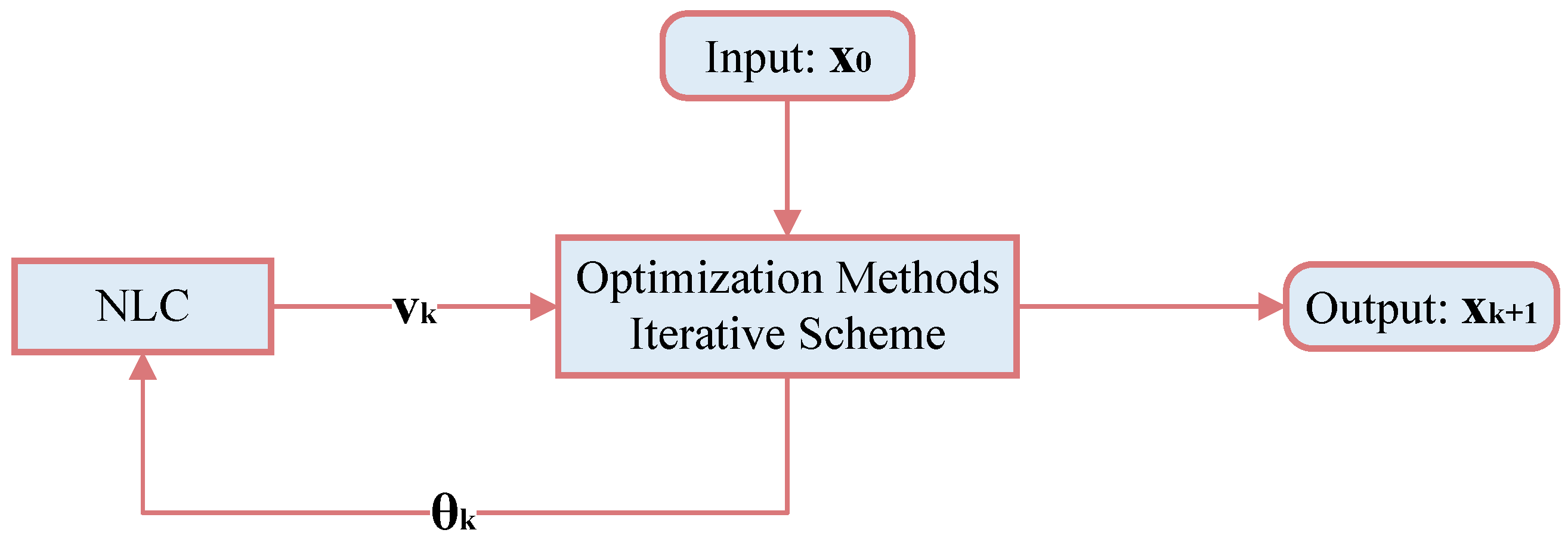
| Input: Objective and an initial point . 1: Put , , calculate , , and generate a descent direction . 2: If stopping indicators are fulfilled, then stop; otherwise, go to the subsequent step. 3: (Backtracking) Determine applying Algorithm 1. 4: Compute using (12). 5: Compute and generate descent vector . 6: (Score function) Compute . 7: (Neutrosophistication) Compute using appropriate membership functions. 8: Define neutrosophic inference engine. 9: (De-neutrosophistication) Compute using de-neutrosophication rule. 10: and go to step 2. 11: Output: . |
FMSM Method
- (1)
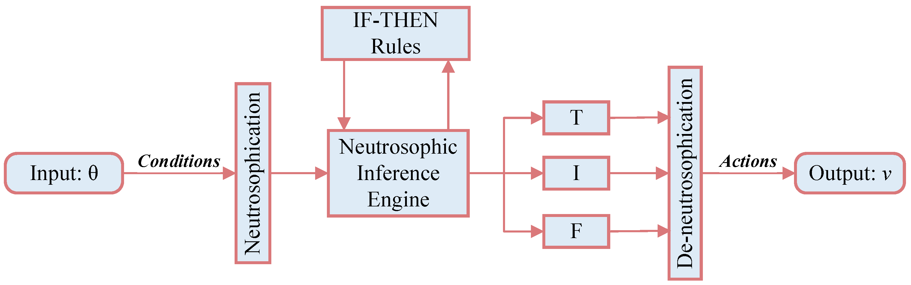
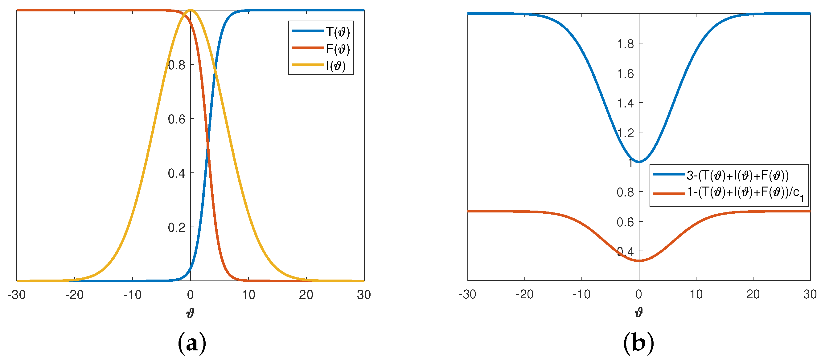
- Neutrosophication. Using three membership functions, neutrosophic logic maps the input into neutrosophic triplets .The truth-membership function is defined as the sigmoid function:The parameter is responsible for its slope at the crossover point . The falsity-membership function is the sigmoid function:The indeterminacy-membership function is the Gaussian function:where the parameter stands for the standard deviation, and the parameter is the mean. The neutrosophication of the crisp value used in the implementation is the transformation of into , where the membership functions are defined in (20)–(22).Since the final goal is to minimize , it is reasonable to use as a measure in the developed NLC. So, we consider the dynamic neutrosophic set (DNS) defined by .
- (2)
- Neutrosophic inference engine: The neutrosophic rule between the fuzzy input set and the fuzzy output set under the neutrosophic format is described by the following “IF–THEN” rules:The notations P and N stand for fuzzy sets and exactly indicate a positive and negative error, respectively. Using the unification , we obtain , , where ∘ symbolizes the fuzzy transformation. Furthermore, it follows that , , and , where ⋀ (resp. ⋁) denotes the operator, (resp. operator). The process of turning the fuzzy outputs into a single, crisp output value is known as defuzzification. There are various defuzzification methods that can be used to perform this procedure. The centroid method, the weighted average method, and the max or mean–max membership principles are some popular defuzzification methods. In this study, the following defuzzification method, called centroid, is employed to obtain a vector of crisp outputs of the fuzzy vector :
- (3)
- De-neutrosophication. This step assumes conversion resulting in a single (crisp) value .The following de-neutrosophication rule is proposed to obtain the parameter using the rule (24), which follows the constraints stated in (13):The parameter maintains the lower limit of in the case . Moreover, definition (24) assumes that the membership functions must satisfy in the case .
| Algorithm 3 Framework of method. |
| Input: Objective and appropriate initialization . 1: Put and compute , and take , . 2: If stopping criteria are satisfied, then stop; otherwise, go to the subsequent step. 3: (Backtracking) Find the step size using Algorithm 1 utilizing the search direction . 4: Compute using (18). 5: Calculate and . 6: Compute applying (19). 7: Compute . 8: Compute using (20)–(22), respectively. 9: Compute using (23). 10: Compute using (24). 11: Put , and go to Step 2. 12: Return . |
3. Convergence Analysis
4. Numerical Experiments
- The CPU time in seconds—CPUts.
- The number of iterative steps—NI.
- The number of function evaluations—NFE.
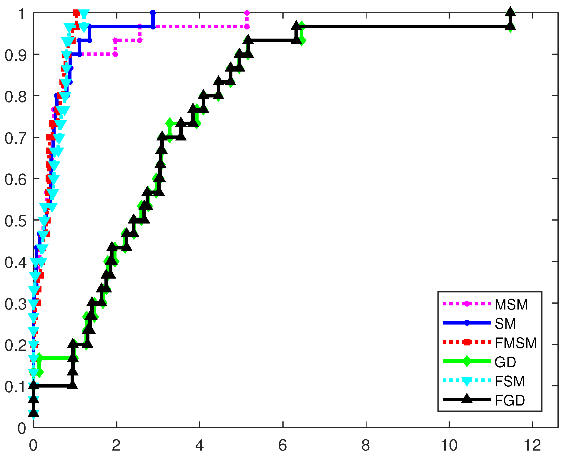
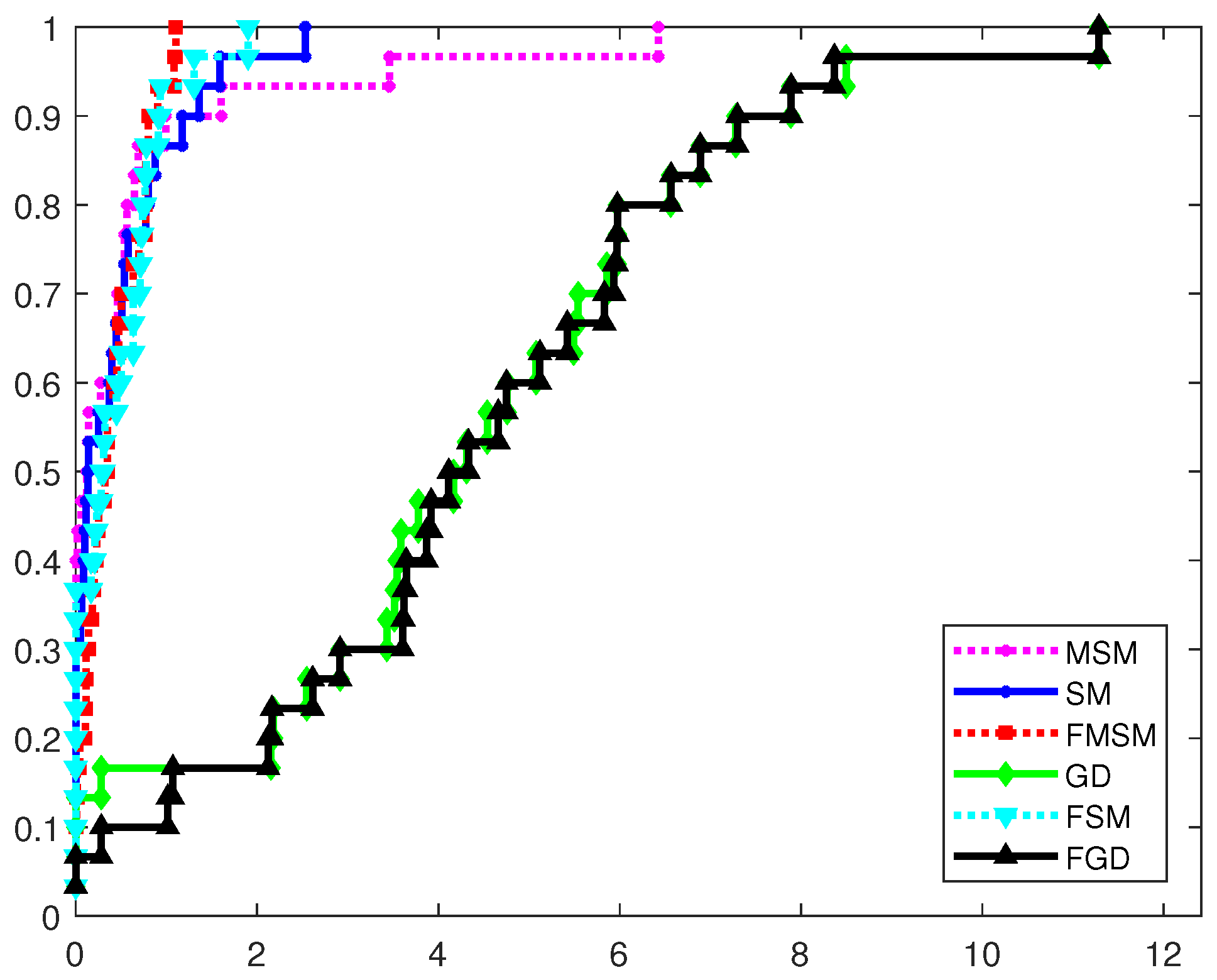
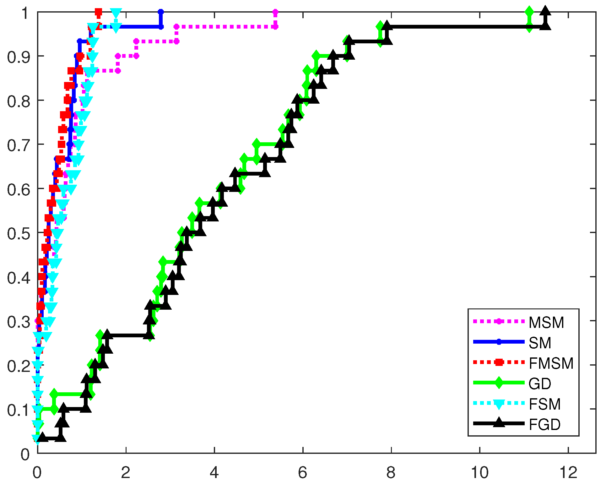
4.1. Comparison Based on the Dolan–Moré Performance Profile
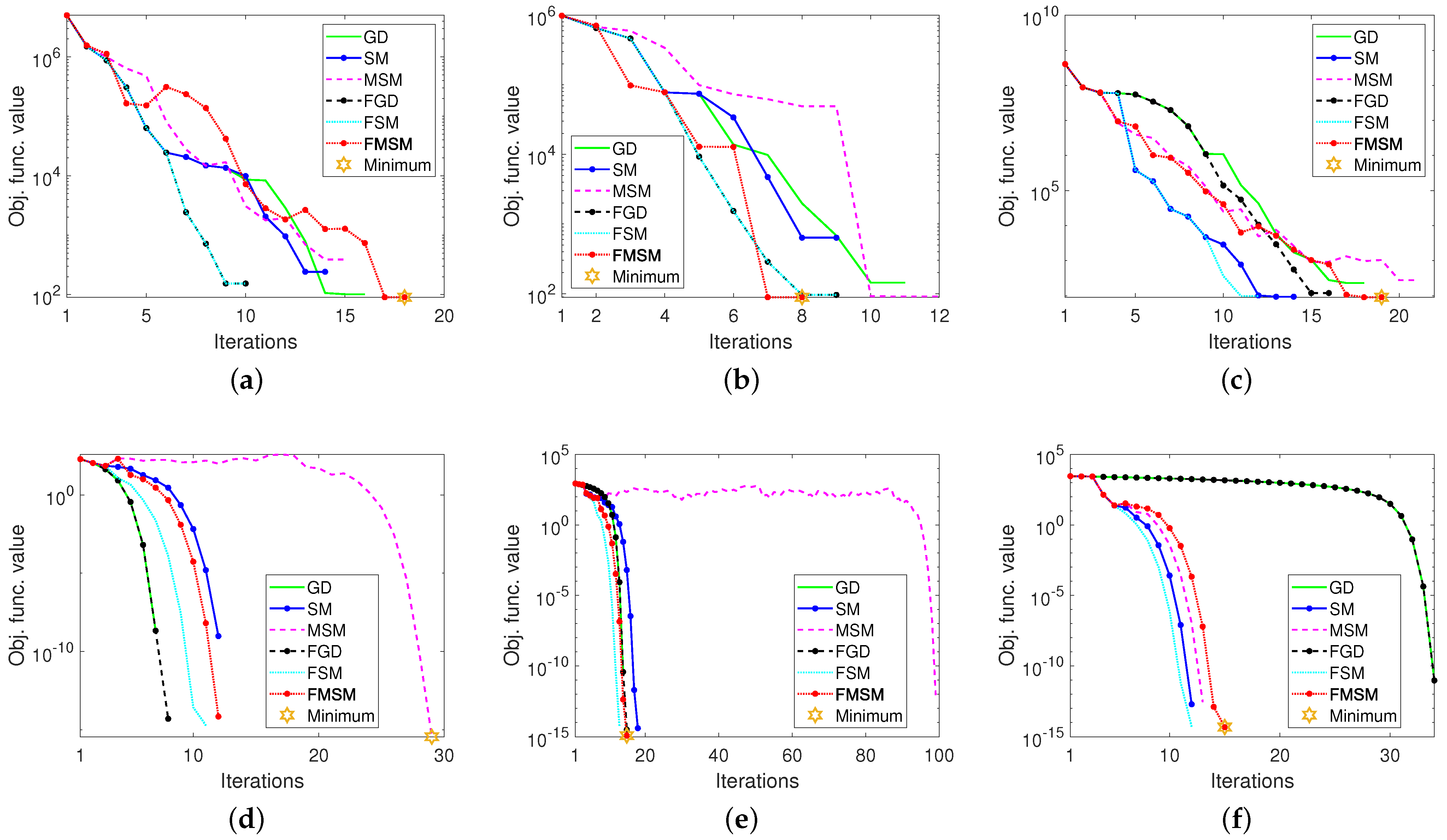
4.2. Closer Examination of the Optimization Methods
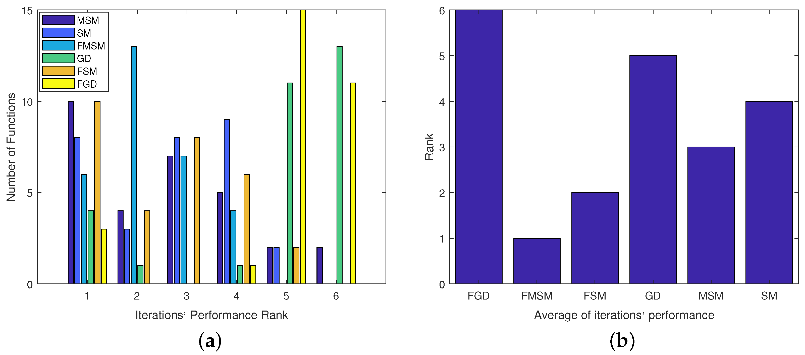
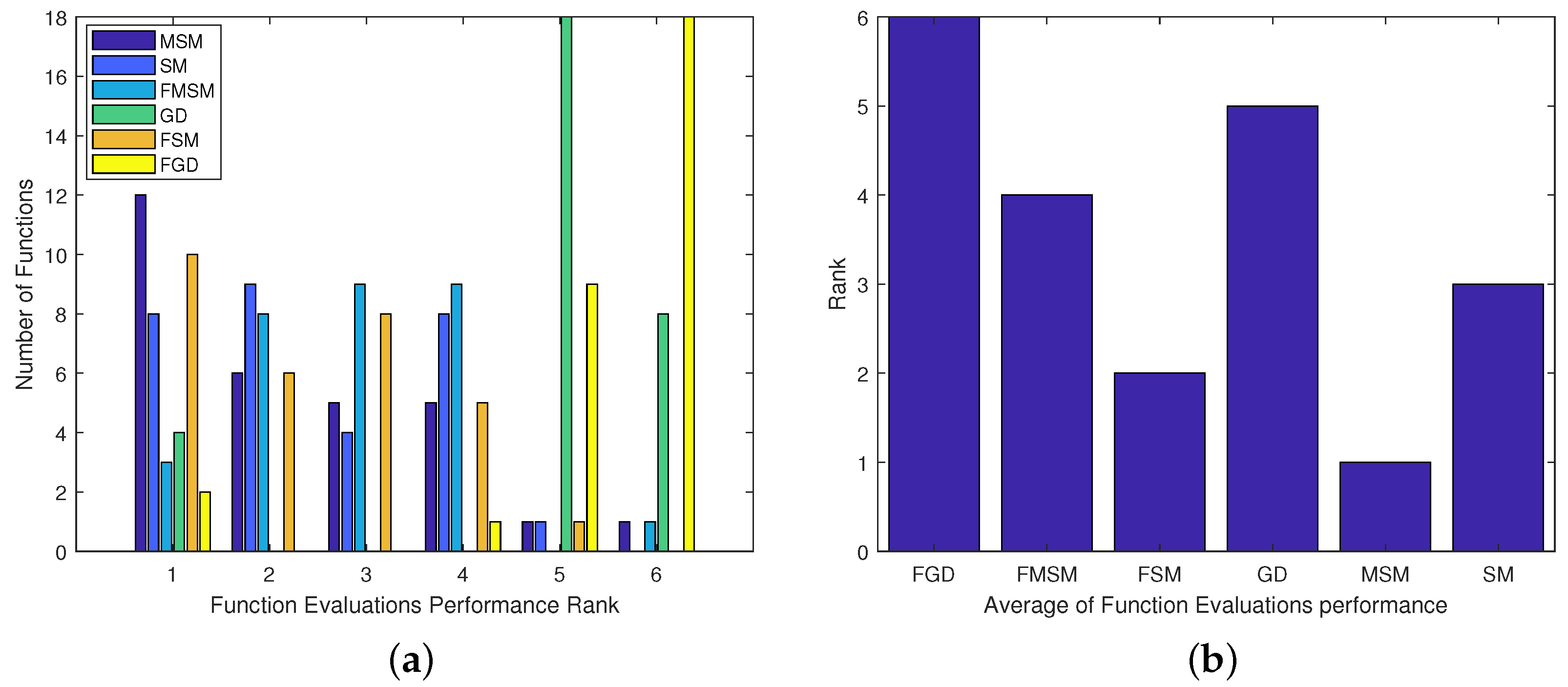
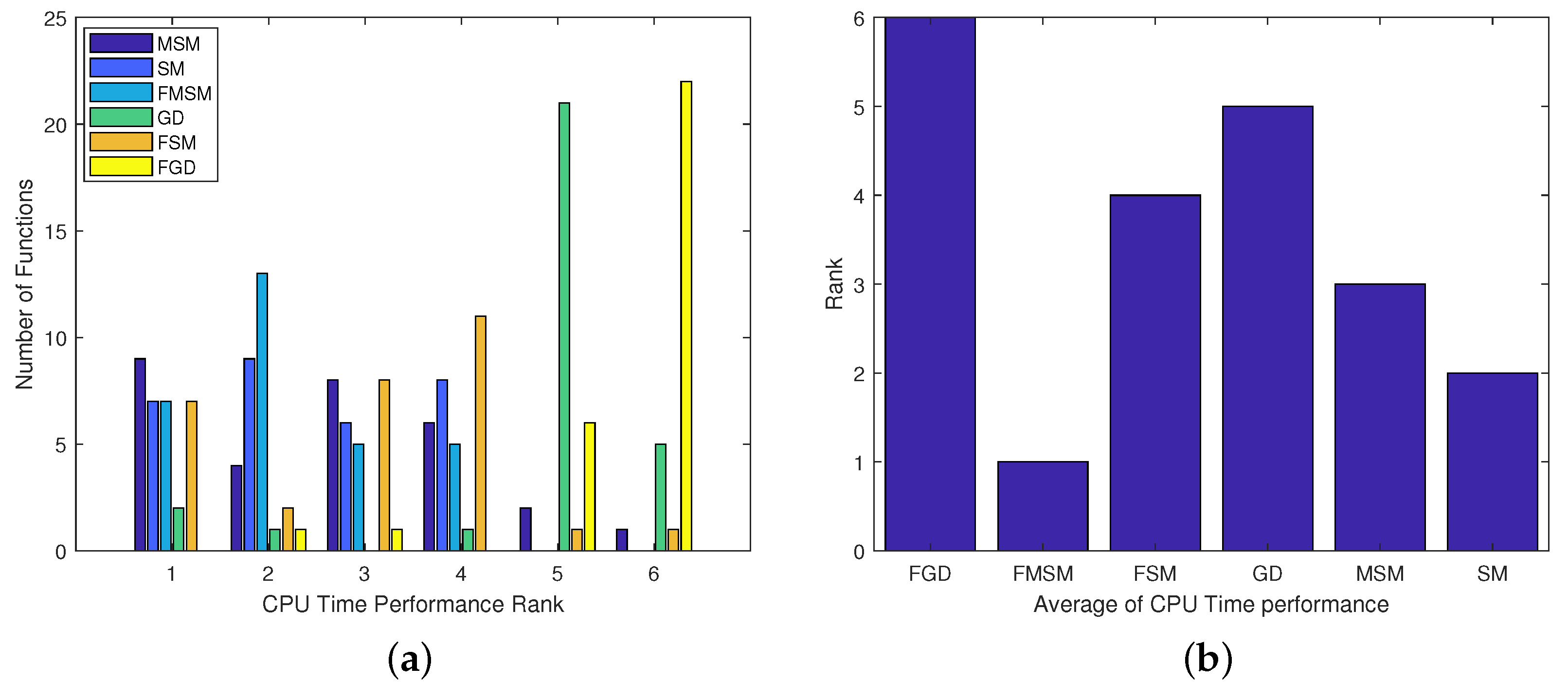
4.3. Ranking the Optimization Methods
- Figure 8b leads to the conclusion .
- Figure 9b leads to the conclusion .
- Figure 10b leads to the conclusion .
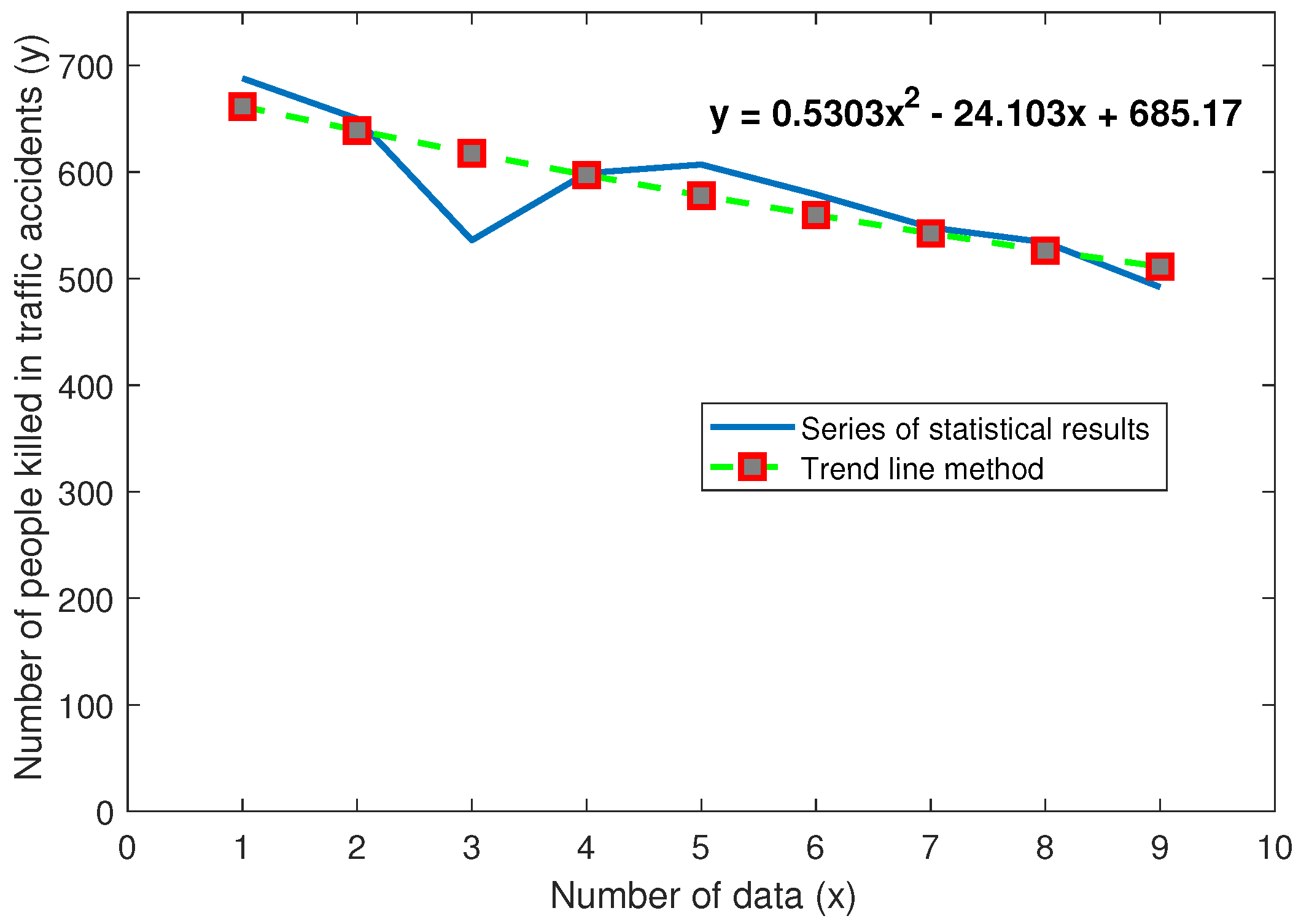
4.4. Application of the Fuzzy Optimization Methods to Regression Analysis
5. Conclusions
Author Contributions
Funding
Data Availability Statement
Acknowledgments
Conflicts of Interest
References
- Sun, W.; Yuan, Y.-X. Optimization Theory and Methods: Nonlinear Programming; Springer: Berlin/Heidelberg, Germany, 2006. [Google Scholar]
- Brezinski, C. A classification of quasi-Newton methods. Numer. Algorithms 2003, 33, 123–135. [Google Scholar] [CrossRef]
- Nocedal, J.; Wright, S.J. Numerical Optimization; Springer: New York, NY, USA, 1999. [Google Scholar]
- Petrović, M.J.; Stanimirović, P.S. Accelerated Double Direction method for solving unconstrained optimization problems. Math. Probl. Eng. 2014, 2014, 965104. [Google Scholar] [CrossRef] [Green Version]
- Petrović, M.J.; Rakocević, V.; Kontrec, N.; Panić, S.; Ilić, D. Hybridization of accelerated gradient descent method. Numer. Algorithms 2018, 79, 769–786. [Google Scholar] [CrossRef]
- Stanimirović, P.S.; Miladinović, M.B. Accelerated gradient descent methods with line search. Numer. Algorithms 2010, 54, 503–520. [Google Scholar] [CrossRef]
- Stanimirović, P.S.; Milovanović, G.V.; Petrović, M.J. A transformation of accelerated double step size method for unconstrained optimization. Math. Probl. Eng. 2015, 2015, 283679. [Google Scholar] [CrossRef] [Green Version]
- Petrović, M.J. An accelerated Double Step Size method in unconstrained optimization. Applied Math. Comput. 2015, 250, 309–319. [Google Scholar]
- Ivanov, B.; Stanimirović, P.S.; Milovanović, G.V.; Djordjević, S.; Brajević, I. Accelerated multiple step-size methods for solving unconstrained optimization problems. Optim. Methods Softw. 2021, 36, 998–1029. [Google Scholar] [CrossRef]
- Petrović, M.J.; Stanimirović, P.S.; Kontrec, N.; Mladenović, J. Hybrid modification of Accelerated Double Direction method. Math. Probl. Eng. 2018, 2018, 1523267. [Google Scholar] [CrossRef]
- Picard, E. Memoire sur la theorie des equations aux derivees partielles et la methode des approximations successives. J. Math. Pures Appl. 1890, 6, 145–210. [Google Scholar]
- Ishikawa, S. Fixed points by a new iteration method. Proc. Am. Math. Soc. 1974, 44, 147–150. [Google Scholar] [CrossRef]
- Khan, S.H. A Picard-Mann hybrid iterative process. Fixed Point Theory Appl. 2013, 2013, 69. [Google Scholar] [CrossRef]
- Rakočević, V.; Petrović, M.J. Comparative analysis of accelerated models for solving unconstrained optimization problems with application of Khan’s hybrid rule. Mathematics 2022, 10, 4411. [Google Scholar] [CrossRef]
- Humaira, M.S.; Tunç, C. Fuzzy fixed point results via rational type contractions involving control functions in complex–valued metric spaces. Appl. Math. Inf. Sci. 2018, 12, 861–875. [Google Scholar] [CrossRef]
- Vrahatis, M.N.; Androulakis, G.S.; Lambrinos, J.N.; Magoulas, G.D. A class of gradient unconstrained minimization algorithms with adaptive step-size. J. Comp. Appl. Math. 2000, 114, 367–386. [Google Scholar] [CrossRef] [Green Version]
- Zadeh, L.A. Fuzzy sets. Inf. Control 1965, 8, 338–353. [Google Scholar] [CrossRef] [Green Version]
- Atanassov, K.T. Intuitionistic fuzzy sets. Fuzzy Sets Syst. 1986, 20, 87–96. [Google Scholar] [CrossRef]
- Smarandache, F. A Unifying Field in Logics, Neutrosophy: Neutrosophic Probability, Set and Logic; American Research Press: Rehoboth, NM, USA, 1999. [Google Scholar]
- Wang, H.; Smarandache, F.; Zhang, Y.Q.; Sunderraman, R. Single valued neutrosophic sets. Multispace Multistruct. 2010, 4, 410–413. [Google Scholar]
- Khalil, A.M.; Cao, D.; Azzam, A.; Smarandache, F.; Alharbi, W.R. Combination of the single-valued neutrosophic fuzzy set and the soft set with applications in decision-making. Symmetry 2020, 12, 1361. [Google Scholar] [CrossRef]
- Mishra, K.; Kandasamy, I.; Kandasamy W.B., V.; Smarandache, F. A novel framework using neutrosophy for integrated speech and text sentiment analysis. Symmetry 2020, 12, 1715. [Google Scholar] [CrossRef]
- Tu, A.; Ye, J.; Wang, B. Symmetry measures of simplified neutrosophic sets for multiple attribute decision-making problems. Symmetry 2018, 10, 144. [Google Scholar] [CrossRef] [Green Version]
- Smarandache, F. Neutrosophic Logic—A Generalization of the Intuitionistic Fuzzy Logic. 25 January 2016. Available online: https://ssrn.com/abstract=2721587 (accessed on 1 September 2021).
- Ansari, A.Q. From fuzzy logic to neutrosophic logic: A paradigme shift and logics. In Proceedings of the 2017 International Conference on Intelligent Communication and Computational Techniques (ICCT), Jaipur, India, 22–23 December 2017; pp. 11–15. [Google Scholar]
- Guo, Y.; Cheng, H.D.; Zhang, Y. A new neutrosophic approach to image denoising. New Math. Nat. Comput. 2009, 5, 653–662. [Google Scholar] [CrossRef]
- Christianto, V.; Smarandache, F. A Review of Seven Applications of Neutrosophic Logic: In Cultural Psychology, Economics Theorizing, Conflict Resolution, Philosophy of Science, etc. Multidiscip. Sci. J. 2019, 2, 128–137. [Google Scholar] [CrossRef] [Green Version]
- Andrei, N. An acceleration of gradient descent algorithm with backtracking for unconstrained optimization. Numer. Algorithms 2006, 42, 63–73. [Google Scholar] [CrossRef]
- Andrei, N. Relaxed Gradient Descent and a New Gradient Descent Methods for Unconstrained Optimization. Visited 29 November 2022. Available online: https://camo.ici.ro/neculai/newgrad.pdf (accessed on 1 September 2021).
- Shi, Z.-J. Convergence of line search methods for unconstrained optimization. App. Math. Comput. 2004, 157, 393–405. [Google Scholar] [CrossRef]
- Ortega, J.M.; Rheinboldt, W.C. Iterative Solution of Nonlinear Equation in Several Variables; Academic Press: New York, NY, USA; London, UK, 1970. [Google Scholar]
- Rockafellar, R.T. Convex Analysis; Princeton University Press: Princeton, NJ, USA, 1970. [Google Scholar]
- Andrei, N. An unconstrained optimization test functions collection. Adv. Model. Optim. 2008, 10, 147–161. [Google Scholar]
- Bongartz, I.; Conn, A.R.; Gould, N.; Toint, P.L. CUTE: Constrained and unconstrained testing environments. ACM Trans. Math. Softw. 1995, 21, 123–160. [Google Scholar] [CrossRef] [Green Version]
- Dolan, E.D.; Moré, J.J. Benchmarking optimization software with performance profiles. Math. Program. 2002, 91, 201–213. [Google Scholar] [CrossRef]
- Dawahdeh, M.; Mamat, M.; Rivaie, M.; Sulaiman, I.M. Application of conjugate gradient method for solution of regression models. Int. J. Adv. Sci. Technol. 2020, 29, 1754–1763. [Google Scholar]
- Moyi, A.U.; Leong, W.J.; Saidu, I. On the application of three-term conjugate gradient method in regression analysis. Int. J. Comput. Appl. 2014, 102, 1–4. [Google Scholar]
- Sulaiman, I.M.; Bakar, N.A.; Mamat, M.; Hassan, B.A.; Malik, M.; Ahmed, A.M. A new hybrid conjugate gradient algorithm for optimization models and its application to regression analysis. Indones. J. Electr. Eng. Comput. Sci. 2021, 23, 1100–1109. [Google Scholar] [CrossRef]
- Sulaiman, I.M.; Malik, M.; Awwal, A.M.; Kumam, P.; Mamat, M.; Al-Ahmad, S. On three–term conjugate gradient method for optimization problems with applications on COVID–19 model and robotic motion control. Adv. Contin. Discret. Model. 2022, 2022, 1. [Google Scholar] [CrossRef] [PubMed]
- Sulaiman, I.M.; Mamat, M. A new conjugate gradient method with descent properties and its application to regression analysis. J. Numer. Anal. Ind. Appl. Math. 2020, 14, 25–39. [Google Scholar]
- Mahmood, T.; Ullah, K.; Khan, Q.; Jan, N. An approach toward decision–making and medical diagnosis problems using the concept of spherical fuzzy sets. Neural Comput. Appl. 2019, 31, 7041–7053. [Google Scholar] [CrossRef]
- Ullah, K. Picture fuzzy maclaurin symmetric mean operators and their applications in solving multiattribute decision–making problems. Math. Probl. Eng. 2021, 2021, 1098631. [Google Scholar] [CrossRef]


| Method | Step Sizes | ||
|---|---|---|---|
| First | Second | Third | |
| GD | - | - | |
| FGD | - | ||
| SM | - | ||
| FSM | |||
| MSM | - | ||
| FMSM | |||
| Set | Membership Function | c | c | Weight | |
|---|---|---|---|---|---|
| Input | Truth | Sigmoid | 1 | 3 | 1 |
| Falsity | Sigmoid | 1 | 3 | 1 | |
| Indeterminacy | Gaussian | 6 | 0 | 1 | |
| Output | (24) | 3 | - | 1 | |
| Test Function | No. of Iterations | |||||
|---|---|---|---|---|---|---|
| MSM | FMSM | SM | FSM | GD | FGD | |
| Extended Penalty Function | 651 | 377 | 549 | 372 | 1255 | 1250 |
| Perturbed Quadratic function | 44,419 | 75,431 | 77,458 | 74,473 | 372,356 | 369,992 |
| Raydan 1 function | 12,965 | 12,437 | 15,913 | 11,035 | 58,743 | 58,594 |
| Raydan 2 function | 90 | 87 | 90 | 94 | 67 | 129 |
| Diagonal 1 function | 52,527 | 11,571 | 8955 | 12,189 | 41,208 | 42,290 |
| Diagonal 2 function | 26,215 | 24,866 | 30,912 | 29,957 | 543,249 | 543,054 |
| Diagonal 3 function | 7545 | 12,586 | 13,892 | 13,050 | 62,128 | 61,072 |
| Hager function | 28,073 | 800 | 839 | 817 | 3104 | 2956 |
| Generalized Tridiagonal 1 function | 290 | 440 | 270 | 376 | 656 | 665 |
| Extended TET function | 130 | 248 | 130 | 225 | 1974 | 1856 |
| Extended quadratic penalty QP1 function | 328 | 189 | 246 | 177 | 563 | 549 |
| Extended quadratic penalty QP2 function | 1538 | 2105 | 3302 | 3564 | 134,401 | 122,926 |
| Quadratic QF2 function | 44,911 | 14,203 | 83,957 | 11,488 | 409,859 | 411,364 |
| Extended quadratic exponential EP1 function | 87 | 100 | 64 | 109 | 496 | 528 |
| Extended tridiagonal 2 function | 568 | 421 | 419 | 415 | 1145 | 1099 |
| Almost perturbed quadratic function | 44,029 | 78,452 | 80,559 | 79,793 | 374,841 | 375,518 |
| ENGVAL1 function (CUTE) | 363 | 298 | 302 | 291 | 573 | 557 |
| QUARTC function (CUTE) | 185 | 216 | 246 | 211 | 524,612 | 524,612 |
| Diagonal 6 function | 90 | 87 | 90 | 95 | 67 | 129 |
| Generalized quartic function | 150 | 150 | 157 | 238 | 1453 | 1751 |
| Diagonal 7 function | 124 | 113 | 90 | 136 | 543 | 570 |
| Diagonal 8 function | 100 | 86 | 103 | 89 | 583 | 573 |
| Diagonal 9 function | 16,920 | 17,221 | 11,487 | 17,752 | 195,362 | 195,155 |
| HIMMELH function (CUTE) | 100 | 90 | 100 | 90 | 90 | 90 |
| Extended Rosenbrock | 50 | 50 | 50 | 50 | 50 | 50 |
| Extended BD1 function (block diagonal) | 189 | 204 | 191 | 223 | 650 | 682 |
| NONDQUAR function (CUTE) | 42 | 39 | 42 | 35 | 33 | 30 |
| DQDRTIC function (CUTE) | 827 | 635 | 1263 | 497 | 15,320 | 15,398 |
| Extended Beale function | 480 | 980 | 639 | 831 | 12,834 | 12,826 |
| EDENSCH function (CUTE) | 337 | 314 | 275 | 275 | 663 | 705 |
| Test Function | No. of Funct. Evaluation | |||||
|---|---|---|---|---|---|---|
| MSM | FMSM | SM | FSM | GD | FGD | |
| Extended Penalty Function | 3527 | 2585 | 2394 | 2388 | 47,378 | 48,057 |
| Perturbed quadratic function | 257,063 | 438,335 | 439,924 | 423,195 | 16,171,466 | 16,069,927 |
| Raydan 1 function | 89,508 | 69,791 | 87,508 | 61,595 | 1,667,238 | 1,658,647 |
| Raydan 2 function | 190 | 233 | 190 | 235 | 144 | 291 |
| Diagonal 1 function | 526,958 | 56,914 | 47,874 | 58,155 | 1,615,828 | 1,664,760 |
| Diagonal 2 function | 158,515 | 144,005 | 171,300 | 166,567 | 1,086,508 | 1,086,118 |
| Diagonal 3 function | 41,528 | 71,024 | 76,336 | 70,540 | 2,407,025 | 2,364,254 |
| Hager function | 271,940 | 3402 | 3308 | 3165 | 56,824 | 54,818 |
| Generalized tridiagonal 1 function | 1012 | 1587 | 931 | 1445 | 10,867 | 11,432 |
| Extended TET function | 440 | 681 | 440 | 601 | 19,800 | 18,859 |
| Extended quadratic penalty QP1 function | 1918 | 1992 | 2507 | 1842 | 10,771 | 11,268 |
| Extended quadratic penalty QP2 function | 10,731 | 14,285 | 24,234 | 26,528 | 3,875,768 | 3,545,317 |
| Quadratic QF2 function | 245,407 | 102,882 | 465,615 | 80,626 | 19,072,367 | 19,141,623 |
| Extended quadratic exponential EP1 function | 807 | 604 | 587 | 830 | 13,643 | 14,852 |
| Extended tridiagonal 2 function | 2550 | 2123 | 2285 | 2111 | 9570 | 9464 |
| Almost perturbed quadratic function | 259,487 | 452,388 | 452,360 | 445,028 | 16,285,621 | 16,309,931 |
| ENGVAL1 function (CUTE) | 1974 | 2700 | 2098 | 2315 | 8787 | 8593 |
| QUARTC function (CUTE) | 420 | 492 | 542 | 472 | 1,049,274 | 1,049,304 |
| Diagonal 6 function | 229 | 335 | 229 | 263 | 158 | 332 |
| Generalized quartic function | 409 | 470 | 423 | 781 | 19,062 | 25,071 |
| Diagonal 7 function | 458 | 547 | 293 | 1094 | 3348 | 4286 |
| Diagonal 8 function | 326 | 462 | 980 | 612 | 3921 | 4078 |
| Diagonal 9 function | 141,781 | 90,948 | 71,353 | 89,023 | 8,449,946 | 8,455,412 |
| HIMMELH Function (CUTE) | 210 | 190 | 210 | 190 | 190 | 190 |
| Extended Rosenbrock | 110 | 110 | 110 | 110 | 110 | 110 |
| Extended BD1 function (Block Diagonal) | 558 | 696 | 598 | 691 | 7660 | 8452 |
| NONDQUAR function (CUTE) | 2084 | 2085 | 2057 | 2060 | 2500 | 2501 |
| DQDRTIC function (CUTE) | 4090 | 2805 | 6518 | 2542 | 395,014 | 400,147 |
| Extended Beale function | 2200 | 4720 | 3277 | 3416 | 207,852 | 208,551 |
| EDENSCH function (CUTE) | 1198 | 1213 | 956 | 872 | 9403 | 10,615 |
| Test Function | CPU Time | |||||
|---|---|---|---|---|---|---|
| MSM | FMSM | SM | FSM | GD | FGD | |
| Extended penalty function | 3.734 | 1.969 | 1.969 | 1.844 | 17.672 | 19.078 |
| Perturbed quadratic function | 167.063 | 323.266 | 298.813 | 317.250 | 10,163.688 | 9771.406 |
| Raydan 1 function | 46.813 | 35.141 | 50.953 | 30.234 | 727.281 | 667.094 |
| Raydan 2 function | 0.453 | 0.281 | 0.281 | 0.344 | 0.250 | 0.531 |
| Diagonal 1 function | 522.703 | 86.500 | 59.297 | 99.953 | 1836.766 | 2091.281 |
| Diagonal 2 function | 236.531 | 228.188 | 271.094 | 276.281 | 2105.219 | 2158.156 |
| Diagonal 3 function | 75.484 | 172.250 | 139.859 | 157.594 | 3842.625 | 4025.688 |
| Hager function | 384.438 | 9.594 | 9.453 | 9.250 | 116.922 | 118.609 |
| Generalized tridiagonal 1 function | 2.656 | 3.188 | 2.000 | 3.797 | 11.641 | 14.875 |
| Extended TET function | 0.953 | 1.313 | 0.906 | 1.359 | 15.922 | 16.281 |
| Extended quadratic penalty QP1 function | 1.688 | 1.625 | 1.875 | 1.578 | 4.203 | 4.391 |
| Extended quadratic penalty QP2 function | 5.844 | 9.891 | 7.203 | 10.516 | 746.328 | 770.500 |
| Quadratic QF2 function | 124.344 | 47.875 | 243.688 | 35.359 | 7611.656 | 8436.359 |
| Extended quadratic exponential EP1 function | 0.969 | 0.594 | 0.469 | 1.109 | 5.281 | 7.297 |
| Extended tridiagonal 2 function | 1.906 | 1.313 | 1.609 | 1.266 | 3.359 | 3.766 |
| Almost perturbed quadratic function | 135.484 | 314.953 | 238.625 | 267.750 | 9271.016 | 13,902.047 |
| ENGVAL1 function (CUTE) | 2.031 | 1.797 | 1.844 | 1.828 | 4.125 | 4.422 |
| QUARTC function (CUTE) | 2.813 | 2.984 | 3.250 | 3.219 | 6253.828 | 8032.547 |
| Diagonal 6 function | 0.328 | 0.219 | 0.344 | 0.484 | 0.203 | 0.438 |
| Generalized quartic function | 0.344 | 0.266 | 0.438 | 0.625 | 6.766 | 11.922 |
| Diagonal 7 function | 0.953 | 0.797 | 0.531 | 1.813 | 3.672 | 4.406 |
| Diagonal 8 function | 0.781 | 0.922 | 1.797 | 1.047 | 5.578 | 4.469 |
| Diagonal 9 function | 249.875 | 74.484 | 53.234 | 77.219 | 2478.422 | 2705.781 |
| HIMMELH function (CUTE) | 0.797 | 0.594 | 0.781 | 0.797 | 0.609 | 0.641 |
| Extended Rosenbrock | 0.203 | 0.094 | 0.156 | 0.203 | 0.219 | 0.141 |
| Extended BD1 function (block diagonal) | 0.766 | 0.766 | 0.859 | 0.969 | 4.984 | 4.469 |
| NONDQUAR function (CUTE) | 7.266 | 8.891 | 7.797 | 9.047 | 9.406 | 10.406 |
| DQDRTIC function (CUTE) | 2.516 | 1.500 | 2.906 | 1.500 | 118.250 | 127.844 |
| Extended Beale function | 7.219 | 18.734 | 9.766 | 16.016 | 488.328 | 546.359 |
| EDENSCH function (CUTE) | 6.141 | 6.422 | 4.016 | 5.063 | 24.672 | 36.766 |
| Average Performances | MSM | FMSM | SM | FSM | GD | FGD |
|---|---|---|---|---|---|---|
| Average no. of iterations | 9477.43 | 8493.20 | 11,086.33 | 8631.57 | 91,962.60 | 91,565.67 |
| Average no. of funct. evaluation | 67,587.60 | 49,020.13 | 62,247.90 | 48,309.73 | 2,416,934.77 | 2,406,242.00 |
| Average CPU time (s) | 66.44 | 45.21 | 47.19 | 44.51 | 1529.30 | 1783.27 |
| Year | Number of Data (x) | The Number of People Killed in Traffic Accidents in Serbia (y) |
|---|---|---|
| 2012 | 1 | 688 |
| 2013 | 2 | 650 |
| 2014 | 3 | 536 |
| 2015 | 4 | 599 |
| 2016 | 5 | 607 |
| 2017 | 6 | 579 |
| 2018 | 7 | 548 |
| 2019 | 8 | 534 |
| 2020 | 9 | 492 |
| 2021 | 10 | 521 |
| Method | Initial Point | NI | NFE | CPUts | Regression Parameters (a, a, a) | ||
|---|---|---|---|---|---|---|---|
| a | a | a | |||||
| FMSM | (1,1,1) | 28,998 | 119,898 | 1.484 | 685.166632504562 | 0.530301492634611 | |
| FSM | (1,1,1) | 29,612 | 120,545 | 1.609 | 685.166666629541 | 0.530303029090458 | |
| FGD | (1,1,1) | 173,004 | 7,861,471 | 35.125 | 685.161769964723 | 0.530114238129987 | |
| FMSM | (5,5,5) | 29,791 | 126,449 | 1.750 | 685.166627004962 | 0.530299060289809 | |
| FSM | (5,5,5) | 29,504 | 119,706 | 1.406 | 685.166666659503 | 0.530303030290009 | |
| FGD | (5,5,5) | 172,876 | 7,855,584 | 36.812 | 685.161745521808 | 0.530113219772043 | |
| FMSM | (−1,−1,−1) | 29,259 | 120,695 | 1.484 | 685.166666761033 | 0.530303033790302 | |
| FSM | (−1,−1,−1) | 29,513 | 119,912 | 1.328 | 685.166388359794 | 0.530292483042678 | |
| FGD | (−1,−1,−1) | 173,698 | 7,893,030 | 37.797 | 685.161987072222 | 0.530122579942827 | |
| Method | Estimation Point | Relative Error |
|---|---|---|
| FMSM | 497.16664 | 0.045745419 |
| FSM | 497.16667 | 0.045745362 |
| FGD | 497.16405 | 0.045750384 |
| Least Square | 497.16667 | 0.045745361 |
| Trend line | 497.17000 | 0.045738964 |
Disclaimer/Publisher’s Note: The statements, opinions and data contained in all publications are solely those of the individual author(s) and contributor(s) and not of MDPI and/or the editor(s). MDPI and/or the editor(s) disclaim responsibility for any injury to people or property resulting from any ideas, methods, instructions or products referred to in the content. |
© 2023 by the authors. Licensee MDPI, Basel, Switzerland. This article is an open access article distributed under the terms and conditions of the Creative Commons Attribution (CC BY) license (https://creativecommons.org/licenses/by/4.0/).
Share and Cite
Stanimirović, P.S.; Ivanov, B.; Stanujkić, D.; Katsikis, V.N.; Mourtas, S.D.; Kazakovtsev, L.A.; Edalatpanah, S.A. Improvement of Unconstrained Optimization Methods Based on Symmetry Involved in Neutrosophy. Symmetry 2023, 15, 250. https://doi.org/10.3390/sym15010250
Stanimirović PS, Ivanov B, Stanujkić D, Katsikis VN, Mourtas SD, Kazakovtsev LA, Edalatpanah SA. Improvement of Unconstrained Optimization Methods Based on Symmetry Involved in Neutrosophy. Symmetry. 2023; 15(1):250. https://doi.org/10.3390/sym15010250
Chicago/Turabian StyleStanimirović, Predrag S., Branislav Ivanov, Dragiša Stanujkić, Vasilios N. Katsikis, Spyridon D. Mourtas, Lev A. Kazakovtsev, and Seyyed Ahmad Edalatpanah. 2023. "Improvement of Unconstrained Optimization Methods Based on Symmetry Involved in Neutrosophy" Symmetry 15, no. 1: 250. https://doi.org/10.3390/sym15010250