1. Introduction
Recently, the research on engineering graphics, which is understood as a set of graphic techniques utilized to solve engineering problems, has been the object of analysis [
1]. Thus, its evolution has been highly notable, and it has been applied in various fields: photogrammetry, reverse engineering, virtual reconstruction, augmented, virtual and mixed reality, image processing and analysis, building information modelling (BIM), computer-aided design (CAD), computer-aided manufacturing (CAM), computer-aided engineering (CAE), bio-models, digital sculpture, rendering and animation, simulation and computer graphics, building, urban planning and historical heritage, shipbuilding, aerospace and industrial construction, cartography, and geographic information systems (GIS), among others. Its inclusion has been especially intense in fields such as CAD [
2], GIS [
3,
4], and CAE [
5], where the existence of a reliable graphical model holds the key to obtaining real simulation results.
On the other hand, from an educational point of view, there have been numerous initiatives to improve the skills of students in the learning and utilization of various competences of subjects related to engineering graphics which comprise the curricula in many engineering fields. There has been research on possible innovations in the practice of teaching engineering graphics [
6,
7], graphic thinking [
8], the teaching of the discipline based on the technique of project-based learning (PBL) [
9], the effectiveness of three-dimensional modelling [
10], and the importance of descriptive geometry [
11], as well as on solving certain mechanical problems [
12]. Likewise, various studies have been carried out on the evaluation of the acquisition of competences, which either highlight the importance of spatial visualization [
13], evaluate the results through an inventory of graphic engineering concepts [
14], or directly establish methods to evaluate the engineering drawings made by students [
15].
From an educational point of view, the development of software that is to be employed in the learning of the discipline has been continuous. For example, various applications have been developed with different programming languages to teach the fundamentals of engineering graphics [
16] and geometric loci as tools to help in the engineering design process [
17,
18].
In engineering, CATIA (Computer-Aided Three-Dimensional Interactive Application) is the most widely used commercial computer-aided design and engineering and manufacturing software. Hence, it is import to teaching this software in engineering schools [
19] and, therefore, convenient for developing educational software. In this way, by seeking the automation of the processes, various applications have been developed in the Visual Basic for Applications (VBA) language, which is the Microsoft Visual Basic macro language employed to program Windows applications, especially for the design of Macros in CATIA [
20]. A macro consists of a series of functions written in a programming language that groups together a series of commands that allow the required operations to be carried out automatically. Among these operations there are applications for the development of sheet metal elbows [
21], for the automatic design of customizable products [
22], and for the automatic design of a cam profile and its fatigue analysis [
23].
The research presented in this article underlines the importance of the application that has been developed from an educational point of view, since it could be used as an evaluation tool for the exercises carried out by students on sections of planes for parts, which is a key process in building different industrial sheet metal parts. Likewise, the application can be programmed to compare the central symmetry of both of the sections (reference section and section that needs to be corrected). To this end, the incorporation of this macro into the CATIA environment could increase productivity by eliminating certain geometric operations.
The remainder of the paper is structured as follows:
Section 2 shows the materials and tools used in this investigation.
Section 3 presents the main process and methods followed in this research.
Section 4 includes the results and discussion, while
Section 5 states the main conclusions and future developments.
2. Materials and Tools
Two types of software have been used in this research: CATIA computer-aided design and engineering software and the Microsoft Excel spreadsheet. These materials differ widely from each other, since each has its own characteristics and functions and, therefore, the instructions that can be given for each also differ. For example, CATIA cannot understand the commands for working with cells that are typical of a spreadsheet, while the latter one has the same problem with the geometry creation tools available in the former one.
2.1. CATIA
As previously mentioned, CATIA enables the creation of macros using VBA. The first step in designing with CATIA, either manually or automatically, is to have an open document to work on. There are different options available in this section: the creation of a new document; opening a document from its file location; utilization the currently active document. Thus, there are commands that allow you to execute each of these options, such as Add and Open. Moreover, it is also possible to automatically save files to the folders once the job is finished.
Subsequently, before being able to generate any type of geometry, it is necessary to open a work module. The macro designed in this research is located inside one of the toolbars of the ‘Part Design’ module, and hence, in order to use it a Part, it must be opened first. To add elements to said Part, it is only necessary to select it using the corresponding instruction.
Performing this action by default works in the main Body, although it could be changed by means of the InWorkObject instruction, if necessary. All the solids that are created are added to this body, and the corresponding Sketches are associated with them. The non-solid elements, such as points and curves, can be added to an existing or new Geometrical Set, which is created in the macro itself. Said Geometrical Set is an object of the HybridBody class.
In order to add an element, such as a Body or a Geometrical Set, the Add instruction is used, while if it already exists and has a name, then the Item command is utilized for its selection:
Set [Object] = [Container].Add
Set [Object] = [Container].Item([Element])
On the other hand, for the creation of geometry, it is essential to previously declare the ToolBox, which contains various tools. For example, to create a point in a sketch, the 2D ToolBox that contains the tools corresponding to the different modes of creating points is needed. To create a geometric element from the corresponding ToolBox, it is only necessary to declare and assign it as follows:
Dim [Name] As [Class]
Set [Name] = [ToolBox]. [Instruction] ([Parameters])
Each ToolBox has different classes of geometric elements that can be created. For example, to create a point in a Sketch, the corresponding class is called Point2D. Regarding the parameters, these can correspond to numerical values (given as a variable of type ‘Integer’ or ‘Double’, etc.) or to another geometric element necessary for the definition. In certain cases, these elements cannot be inserted directly from the object that defines them, but they must be transformed into another object of the type ‘Reference’.
2.2. Microsoft Excel
Microsoft Excel also enables the creation of macros using VBA. Furthermore, actions can be programmed in said spreadsheet by the CATIA editor. This is very useful in terms of taking advantage of the possibilities of both of the materials and combining them. The spreadsheet enables all types of data to be entered in a row and column format. Moreover, operations can be performed with the spreadsheets, and graphs can be generated, among many other possibilities.
To open said spreadsheet using CATIA, the following lines are used:
Set [Document] = CreateObject(“Excel.Application”)
Set [Workbook] = [Document].Workbooks.Add
Such a spreadsheet is made up of cells, which are labelled as rows and columns. In order to call these cells, it is necessary to indicate these two parameters through two different commands: Cells and Range.
The Cells command requires two numeric parameters as the input, while Range uses a single ‘String’-type input parameter. This entry uses letters for the columns and numbers for the rows, such as ‘A1’. Furthermore, the entire ranges can be selected by checking the top left hand side and bottom right hand side boxes.
[Document].Range(“[Cell1]:[Cell2]”).[Instruction]
To enter these data, the Value property of the Cells and Range classes is utilized, in accordance with the line model indicated above. This system, in which the action takes place after the specification of the cells, is valid for all of the commands that require a single range of cells to be inputted.
Among the various actions that can be carried out, it is worth mentioning the application of formulae and the change in the format of the cells. Moreover, one of the most powerful applications of said spreadsheet, those of the ability to auto-fill the cells, can also be programmed in VBA.
To enter a formula, it must be typed in the same way as it is in the command bar of a spreadsheet. Here is an example:
[Document].Range(“[Cell]”).Formula = “=SQRT((D4-F4)^2 + (E4-G4)^2)”
Likewise, it is important to highlight the use of the equal sign before the introduction of the formula, which must be written in the data string format.
The same instructions are employed to format the cells, but with the corresponding commands. For example, Merge is utilized to merge the cells, while Interior.ColorIndex enables the interior of the cells to be colored.
On the other hand, the auto-filling of the cells requires two ranges: one that indicates the cells where the data that will work as an example are found, and another one that is the filling.
[Doc].Range(“[Range1]”).AutoFill Destination: = [Doc].Range(“[Range2]”)
3. Process and Methods
The processes carried out by the macro can be divided into four blocks, which are executed in the following order: the development of a basic interface, the calculation of the real section in CATIA (reference section) and its dihedral projections, the import of the external file (section that needs to be corrected), and the comparison between both of the results.
The acquisition and representation of the sections supposes the greater part of the development of the macro. Each of these blocks is obtained from two different sources using different methods. Therefore, its code is fundamentally different and its development is separated into two different blocks.
The objectives of each of these blocks are indicated below, and the process and methods that compose them are developed.
3.1. Graphical User Interface (GUI)
The graphical interface is a key element of the macro that enables the user to introduce the necessary data for its operation. The VBA editor enables the elements that comprise it to be manually placed in the windows, and its operation and internal relationships are subsequently programmed.
In the final result, the graphic interface changes its appearance and available elements depending on the method of introducing the secant plane through the coordinates of three non-aligned points and by the direct selection of an already defined plane.
Each of these methods needs different input parameters. On the one hand, in the case of entering the coordinates of the points, only nine text entries are needed, one for each coordinate of each point, while on the other hand, in the case of the selection of the plane, it must be possible to select an element of the appropriate type from the CATIA screen. Due to these differences, it is necessary to create two versions of the graphical interface and create a system for their selection. The system chosen involves a drop-down menu which, subsequent to the user’s selection, executes a code that hides the window on the screen and shows the chosen one.
In this case, with only two programmed methods, there are simpler systems for choosing the section method by the user. However, before the possible future addition of new methods, the drop-down menu is the most comfortable and fastest system, whose name in VBA is Combo Box.
The only differences between the windows are found in the data of the secant plane for the calculation of the reference section using CATIA.
In addition to the aforementioned Combo Box, other types of very frequent widgets such as Text Box and Buttons are used.
3.2. Reference Section
This block absorbs most of the execution time of the macro, since it contains both of the actions related to the modification of the geometry in CATIA and an iterative process. Furthermore, this is the only block that is affected by the differences in the input data in the graphical interface. In turn, this entire process can be subdivided into modules, which are analyzed below.
3.2.1. Creation of the Section in Its Plane
This block defines the plane with which the section is generated in the part. Therefore, the choice of the plane definition method does not affect the rest of the macro, since in the end, it will only need the object associated with the plane, regardless of how it was obtained.
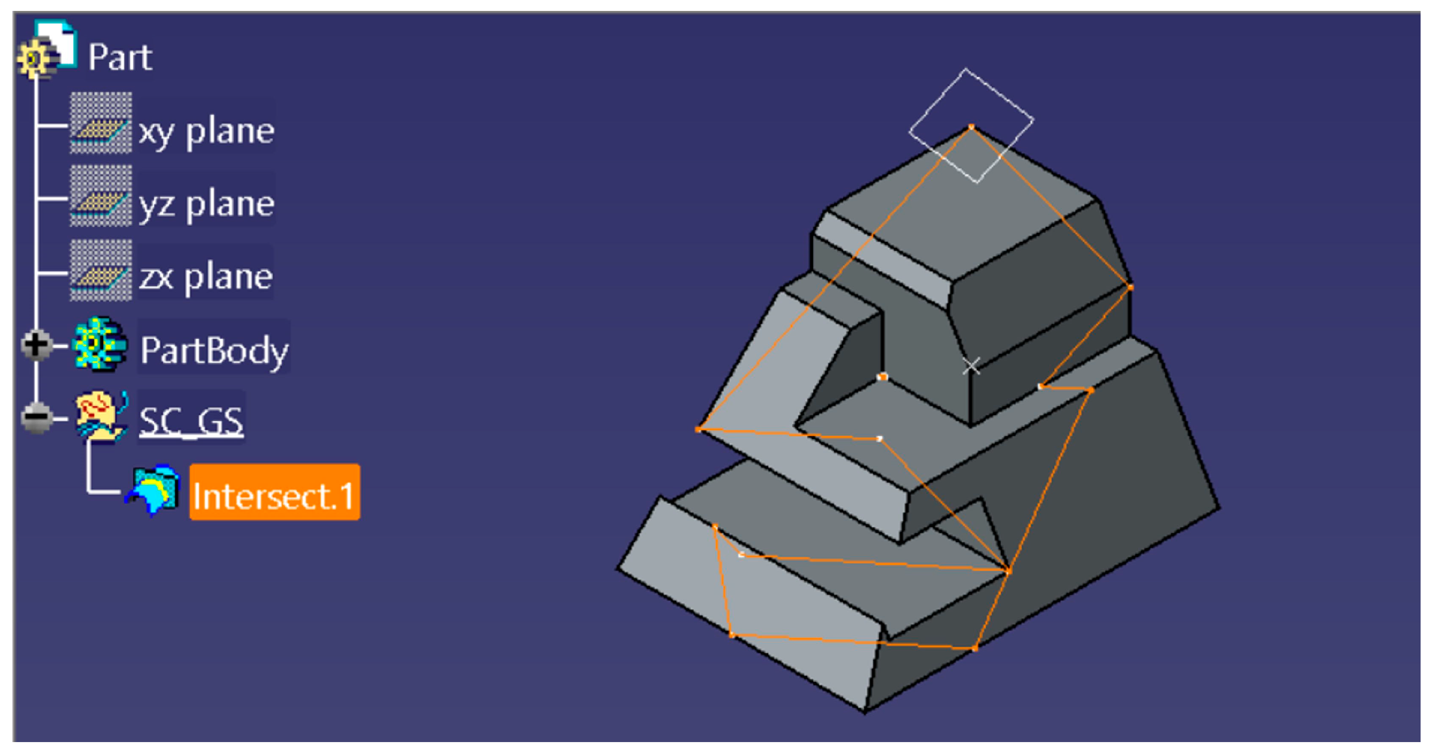
The acquisition of the reference section is based on using CATIA to perform the intersection between the plane and the part entered into the macro as inputs. To this end, the
AddNewIntersection command is utilized, which corresponds to the
Intersect instruction. This command, which is associated with a
3D ToolBox, requires the input data of two objects which must intersect with the reference format. If the part consists only of planar faces, then the result will be one or more closed polylines. This polyline is stored in the CATIA operations tree as a single element (
Figure 1), and hence, it is necessary to disaggregate its comprising lines.
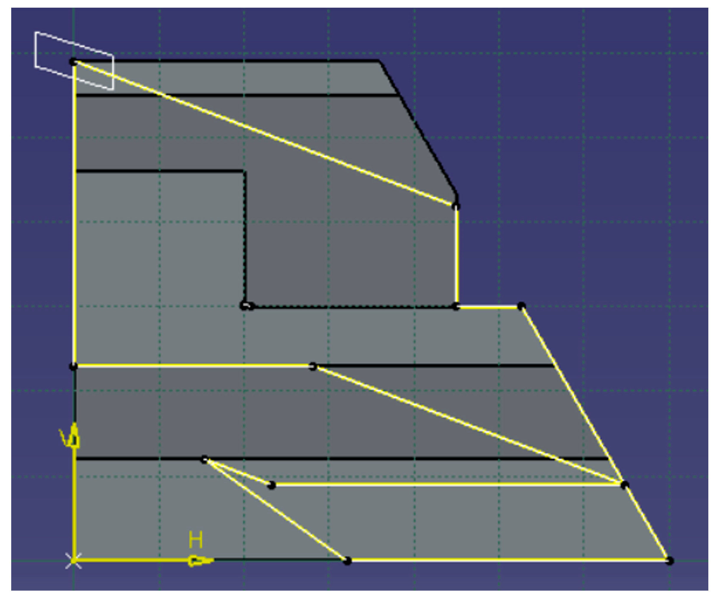
This operation can be carried out by proceeding in one of two ways: either we program a function that analyses the individual elements with line format that make up the polyline and create a new line for each element, or we use the
Disassemble command of the CATIA module ‘Wireframe and Surface Design’ (
Figure 2). This latter mode presents a drawback that no instruction exists in VBA that performs this function, and hence, it would be necessary to respond to said command as if it were to be performed manually.
In the macro carried out, the second option was chosen, in accordance with the following steps:
Set the intersection as the only selection. The reason for this step is that this command, if it is activated with an element selected, is automatically applied to that selection.
Use the CATIA Disassemble command.
Accept the application to all of the elements that make up the polyline. The Disassemble command displays a new window before performing its function. In this window, a selection is required as to whether disaggregation is desired of all of the elements or only in terms of the domains. By default, the option of all of the elements appears, and therefore, it is only necessary to accept this system. To this end, the ‘OK’ button in the window itself or the ‘Enter’ key on the keyboard can be pressed. To program this second option, the VBA statement SendKeys is utilized.
Halt the execution of the macro for a short period to allow time for the execution of the Disassemble command.
Update the Part.
3.2.2. Acquisition of the Dihedral Projections of the Section
The projection of the section in each of the dihedral projections of the part (
Figure 3) is made in a
Sketch placed in the appropriate planes. The CATIA ‘Sketcher’ module presents a function that allows the perpendicular projection of the geometry external to the
Sketch itself to occur. Said command is called
CreateProjection, which belongs to the
2D ToolBox, and like most instructions of this class, it requires the geometric elements to be entered as references.
In order to create the references and projections, the lines are grouped in a vector-type object. In this way, the problem arising from the fact that the number of lines that make up the section is not the same in all of cases is thereby solved. Although VBA needs to be informed of the length of the vectors that are used, it allows a vector of undefined length to be defined, and then, its definition is achieved using the ReDim statement. The dihedral projections of each vector line are made in an external function that is repeated for each of the dihedral projections of the part.
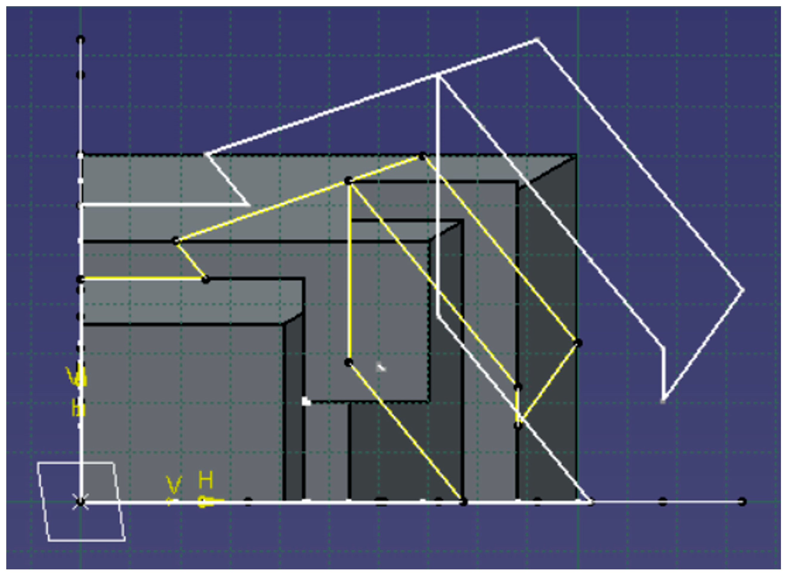
3.2.3. Visibility Study
The study of the visibility of each of the lines is the analysis of the intersection generated with CATIA. This analysis is necessary to guarantee the reliability of the results shown in the spreadsheet, since the external file that contains the section that needs to be corrected will contain the visible and hidden sections with different line formats. This means that a line with a visible stretch and a hidden stretch will have to be stored as two different lines in that file. It is therefore necessary to find the point at which said visibility change occurs in order to separate the lines of the reference section in accordance with this criterion, which is not contemplated in the CATIA solution.
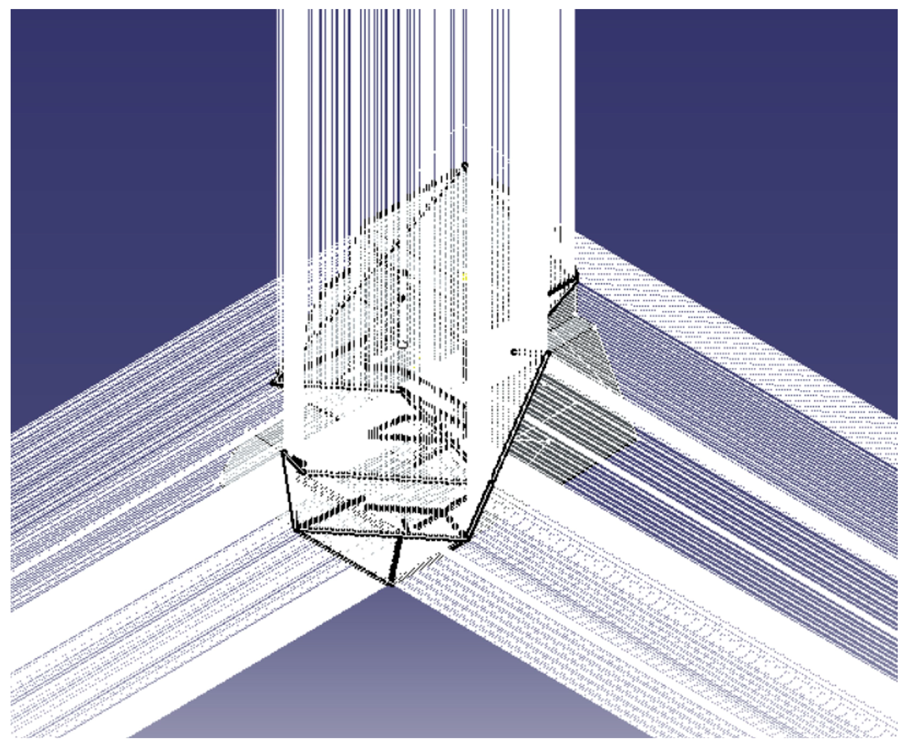
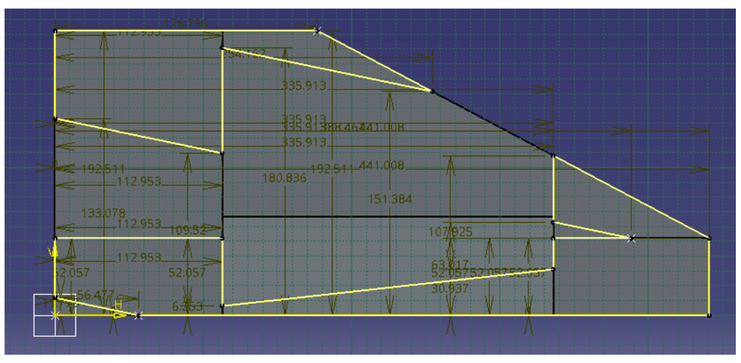
For a geometric element to be visible, the only condition is that no other element is located between said element and the observer. Thus, the algorithms under study are based on the location of possible objects in one direction from the element in question, and to this end, lines are used that originate from a point of said element in the appropriate direction (
Figure 4). The existence or non-existence of intersection points in this line with other external geometric elements determines the visibility of the object.
Said algorithms require the geometry to be discretized for the execution of the analysis. In this case, the division of the lines into smaller elements (sections) can be performed, for example, by setting the distance of said sections or the number of sections per line. However, regardless of the method used, many divisions are needed to achieve a high level of precision. A high number of elements and actions is implicit in this type of algorithm, and it means that the precision of the process is closely related to the computational cost and the execution time that are required.
However, the result that is shown, in which all of the timelines utilized by the algorithm can be observed, makes it difficult to visualize the section and its dihedral projections. For this reason, they should be deleted once the macro has finished running. To this end, a specific Geometrical Set is created to store the temporary elements, so that they can all be conveniently removed at the end of the process.
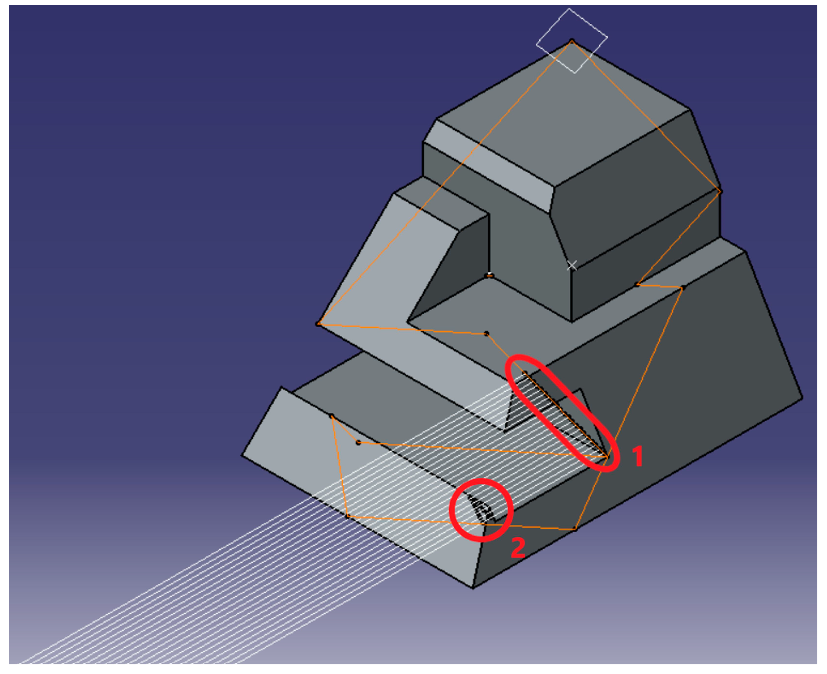
Finally, the most important aspect of the algorithm is the determination of the existence of intersections in the lines. To this end, a method based on the length of the lines is employed. The basic process consists of cutting the lines if they intersect the part using the CATIA
Split function. The length of the line before and after the section is then compared. If there is a difference between the two elements, then the analyzed point must be hidden behind another part of the piece (
Figure 5).
In this figure, the execution process of the visibility analysis function applied to a straight line can be observed. On the one hand, Mark 1 shows the points from which the lines initially originate, resting on the intersection of the plane with the part, and hence, the separation between these points defines the precision of the process. On the other hand, Mark 2 highlights the existence of points created at the intersection of the lines and the part. These points mark the cuts of the lines, which shorten their length.
The visibility function saves the information of all of the lines in a vector of Boolean components, which returns the value ‘True’ if there is visibility at the corresponding point, and ‘False’ if this is otherwise. Subsequently, said vector acts as an input in the function in charge of placing the data of the section obtained with CATIA (reference section) in the spreadsheet. This function analyses the vector by seeking changes in the value of two consecutive components that do not correspond to a corner. Once these changes have been found, and given the position corresponding to each component, the straight line can be divided into the necessary sections.
3.3. Section That Need to Be Corrected
The section that needs to be corrected must be given in an external file in the dxf format (Drawing eXchange Format), which is a data exchange format for vector-type planar drawings. The DXF file can be obtained by any CAD software that allows conversion to take place from its native format to the DXF format. CATIA enables these files to be imported in the ‘Drafting’ module. However, information is lost during the import process since CATIA in this module fails to present all of the functionalities available in the other software. For example, this module does not distribute the information in layers, and therefore, if the file has this distribution, then all of the layers are unified into a single layer.
Said external file holds each dihedral projection of the section in different layers, and it has, therefore, been decided that it should read the file as text and extract the data as character strings of the corresponding lines. To this end, the text is traversed line by line and the necessary data are stored.
The dxf format, which is used to indicate the properties of a line, presents a well-known structure that is headed by the ‘Line’ instruction. The following lines specify the graphic properties, the layer to which it belongs, and the start and end points. In this way, the line is completely defined.
However, before these lines can be represented in the corresponding Sketches, the imported geometry needs to be translated and resized. On the one hand, the appropriate Sketch is selected when we are entering the data into the interface in the ‘Layers’ section. The macro needs to acquire the names of the layers to read the data from the dxf file and associate it with the correct dihedral projection of the part. On the other hand, said translation is carried out by adding the distance to the original coordinates. Therefore, to calculate the translation distance, an initial iteration is carried out to locate the closest point to each of the axes, that is, the dihedral projections of the section are placed in contact with the axes, which implies the application of a condition to the situation of the input geometry. This condition consists of placing the part in the positive octant of three-dimensional space, with a face or vertex that is in contact with each of the XY, YZ, and XZ coordinate planes.
Finally, the resizing is performed by dividing the original value of the coordinates by a scale parameter, which is provided as an input to the macro.
On carrying out these transformations, if the section that needs to be corrected (external file) is correct, then the dihedral projections of the reference section and of those to be corrected visually coincide.
3.4. Data Comparison
Since the application software checks only the dihedral projections of the sections, with the joint representation of the dihedral projections of both of the sections, the level of coincidence can be visually appreciated. However, the accuracy analysis would be purely qualitative. In order to obtain quantitative results, the data of the lines are exported into a spreadsheet, in which said data can not only be analyzed more easily, but they can also operate to obtain values of the error that occurred.
3.4.1. Acquisition of Coordinates
As previously mentioned, the methods used to obtain and represent the lines that make up the sections differ considerably. On the one hand, in the reference section, the lines are obtained directly, while those in the section that need to be corrected are represented by their initial and final points.
For the numerical characterization of the lines, the section that needs to be corrected has the advantage that the coordinates of the start and end points are already known. These data completely characterize the line, and they can therefore be automatically used in the spreadsheet. However, the lines of said reference section do not have numerical values, only their representation in CATIA, and hence, to obtain the value of these data, the creation of
Constraints (
Figure 6) is achieved for each start point and end point of each line.
Finally, the calculations and the export of the numerical data are performed together with the representation, so that unnecessary loops are prevented.
3.4.2. Sorting Lines and Points
The coordinates are exported to a spreadsheet, whose data table format enables comfortable handling and easier visualization when the number of points is high. The rows of this table contain the initial and final points of each line, while the different characteristics of the points or lines (coordinates and errors, etc.) are placed in the columns. The number and position of the columns are known, and they are fixed by the desired number of variables stored regarding the lines and the necessary ordering. However, each dihedral projection of the section comprises a different number of lines, and their position does not follow a fixed order that is established in advance. It is therefore necessary to identify the number of lines and apply an ordering that enables the comparisons to be made correctly. In this section, two different orders must be distinguished:
Firstly, it is necessary to make the comparisons between the appropriate lines, and secondly, if a comparison between the position of the points is required, then it is necessary that the identification of the initial and final points also correspond to each other. This distinction is not important for the length since this does not vary, while if the angle accounts for only the orientation of the line and not the direction, then the arrangement of the initial and final points causes no effect either.
In order to carry out these two orders, it is necessary to define the criteria as follows. Thus, to organize the lines, the arrangement of the elements in the CATIA operations tree is used, that is, the lines are placed one by one in the spreadsheet during data extraction, and subsequently, the data of the external file (the section that needs to be corrected) can be located based on the previous data.
To this end, a comparison code is used that analyses each line of the section that needs to be corrected one by one by studying the error of the coordinates of the points. In this way, each line of the section that needs to be corrected is associated with the closest line of the reference section.
If the data matched perfectly or there were only small errors in the points, then this criterion would suffice. However, it is possible that there will be missing lines or lines that are widely displaced with respect to the real lines, which could cause several lines whose best fit is a single line of the spreadsheet. In order to avoid this situation, an additional check is performed, consisting of comparing the error of both of the straight lines with the straight line of the reference section, if this were the case. The line that has the smallest error is considered to be the correct one, and we place the other line in another position if there is one.
Likewise, to decide which point is designated as ‘initial’ and which point is designated as ‘final’, its distance from the origin is measured. The point with the lowest value of this parameter is considered to be the initial point, regardless of how it is connected to other lines.
3.4.3. Calculation of the Error Committed
Four different line error calculations have been implemented in the spreadsheet: errors in the coordinates of the points, in their length, in the angle with respect to the horizontal, and in their visibility.
These errors are obtained directly from the spreadsheet, whereby the corresponding formulae are programmed in the cells dedicated to displaying these data. The main advantage of using spreadsheet formulae is the ability to manually change the data once the software has finished, so that the error is updated automatically.
Each cell dedicated to an error is also associated with a specific line, which means that these four different errors are calculated for each of the straight lines of each of the three dihedral projections represented. In order to obtain values of a more generic nature, the mean of each of the types of errors is obtained for each straight line, and in this way, there are only four error values per projection.
Furthermore, during the execution of the software, it is necessary to make comparisons with these errors to order the lines in the spreadsheet. These errors, which are not shown among the final results, are calculated internally in the VBA code using the same formulae that are entered in the spreadsheet.
Error in the Coordinates
This error refers to the distance between the points that should coincide if the external file containing the section that needs to be corrected has no discrepancies compared with that obtained from CATIA (reference section). That is, each pair of points in the same row of the spreadsheet is analyzed, for example, the initial point of the straight line obtained in the reference section is compared with the initial point of the section that needs to be corrected (external file).
The formula employed to measure this error represents the distance between two points on a plane, which is also utilized to calculate the length of lines from the coordinates of their extreme points.
Finally, so that the errors are equivalent for the parts of different sizes, it is rendered dimensionless regarding the length of the line of the reference section. That is, the error in the coordinates is a relative error with respect to the length of the line to which it refers, however, it should be clarified that since the lines have different lengths, the value with which it is relativized is not the same in all of the lines.
Error in the Length
The error in the length of each line is another relative error, which is calculated by dividing the difference in length by the value of this same magnitude for the line of the reference section.
Error in the Angle
The error in the angle refers to the difference in the inclination of each line with respect to the horizontal plane. For this calculation, the value is not divided, and it maintains angular units (sexagesimal degrees). The reason why this division is not carried out is due to the characteristics of the angles.
Visibility Error
This error shows the similarity or difference between the visibility parameters of two corresponding lines, one is from the reference section and the other one is from the section that needs to be corrected. Since they are Boolean variables, the visibility error should simply compare whether they are equal or not. This is carried out by subtracting them from each other, such that a null result implies that there is no error. Moreover, an absolute value is applied to the result so that the existence of error always has a representation of value 1.
4. Results and Discussion
The final result is an integrated application (SectionCheck) in the form of a macro in CATIA V5R21, which was developed with the CATVBA language. Its function is to locate and quantify errors in the dihedral projections of a section of a plane to a part, which is stored in a dxf format file. Likewise, to facilitate its use, the possibility of accessing it by means of a button located in a specific library has been added.
All of these details are presented below by way of an explanatory manual of the process, the options, and the results of the application.
4.1. Operation of the Application
4.1.1. Create or Import a Solid in CATIA
The first step involves generating the 3D CAD model, in which the section is to be made. Its location in the CATIA coordinate system is important, since for the application to work correctly, the 3D CAD model must be completely contained in the octant of space, in which all of its coordinates are positive. Likewise, it must have at least one point in each of the three coordinate planes that define the system (X = 0, Y = 0, and Z = 0), and the orientation must be such that the observer is located in the positive part of the axes to see each of the views. The plane to which each view corresponds is chosen using an option that is explained later.
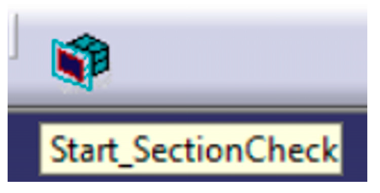
4.1.2. Start of the Application
In order to start using the application, the ‘Start_SectionCheck’ button must be used (
Figure 7). This button is located on the ‘Developed Macros’ toolbar, although it is possible to modify this location from the ‘Customize’ window of the ‘Tools’ menu.
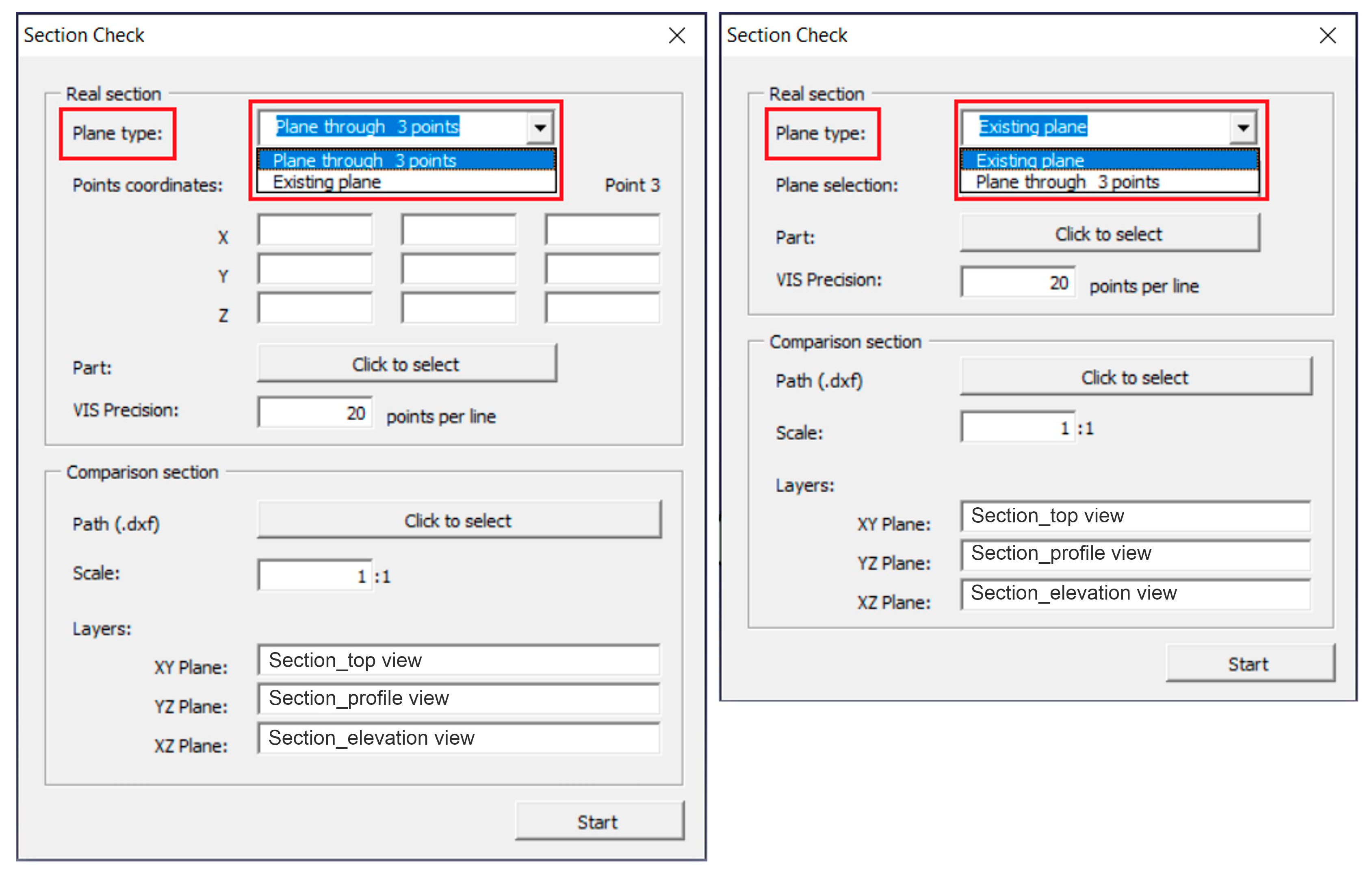
4.1.3. Selection of the Secant Plane
This action is performed from the ‘Plane type’ drop-down menu, belonging to the ‘Real Section’ group, for which there are two possibilities (
Figure 8):
The definition of the plane through the coordinates of three non-aligned points (
Figure 8, left -hand side), which is the default option.
The selection of a plane previously defined in CATIA (
Figure 8, right -hand side).
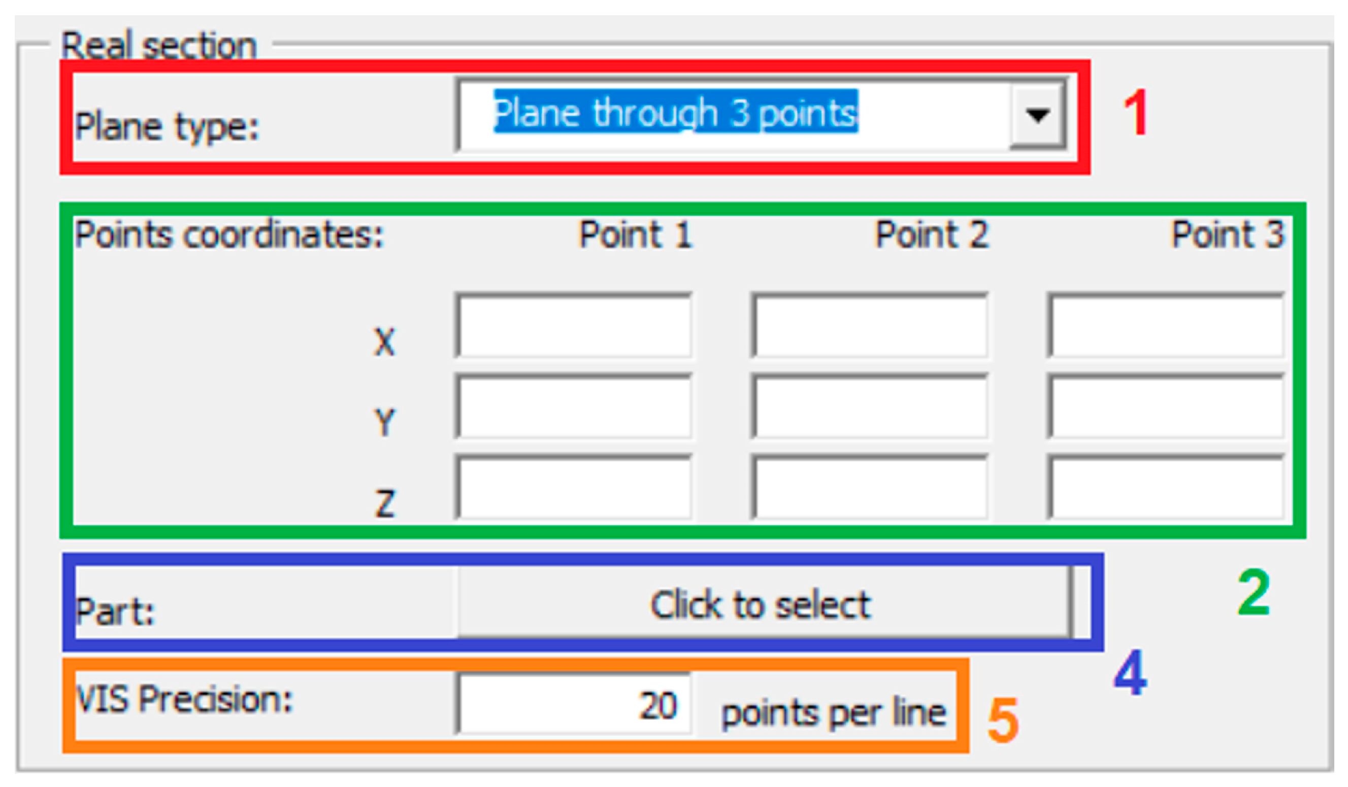
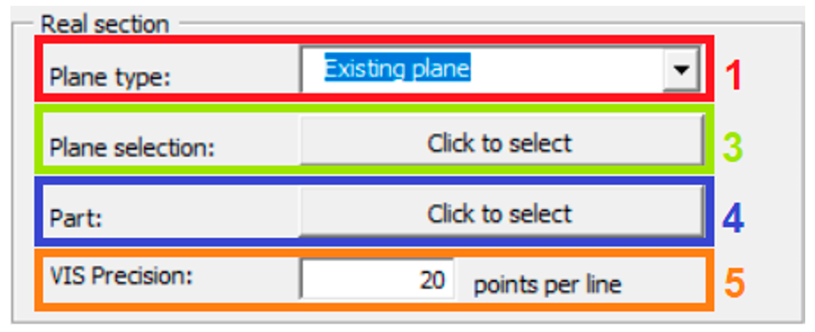
4.1.4. Introduction of Parameters for the Section Generated by CATIA (‘Real Section’ Group)
- 1.
Plane Type (
Figure 9 and
Figure 10, Mark 1): the selection of the method for entering the secant plane.
- ○
Point coordinates (
Figure 9, Mark 2): Cartesian coordinates of three non-aligned points contained in the secant plane. The origin of coordinates is that of CATIA. This set of parameters is activated by clicking on the ‘Plane through 3 points’ option in the ‘Plane type’ drop-down menu. Each column represents the coordinates of one of the points. The method of entering the points is performed by using the keyboard, selecting the corresponding box with the mouse, or by using the tabulator.
- ○
Plane Selection (
Figure 10, Mark 3): The selection of an existing plane in CATIA. This button appears when one has activated the ‘Plane selection’ option in the ‘Plane type’ drop-down menu. Pressing the button hides the interface and enables a plane to be selected.
- 2.
Part (
Figure 9 and
Figure 10, Mark 4): Selection of the part that will be sectioned by the plane to obtain the section. Its operation is identical to that of the ‘Plane selection’ button.
- 3.
VIS Precision (
Figure 9 and
Figure 10, Mark 5): The number of equally spaced points in which the visibility of each line of the section is analyzed. Its range is limited between five and one hundred, with twenty being the default value. Increasing the number of divisions improves the detection accuracy of the visibility changes at the cost of increasing the execution time of the macro. For a section with many straight lines, increasing this parameter excessively if one desires the fast execution of the application is not recommended. The default value of twenty divisions represents a balanced process between precision and speed for sections that have between ten and twenty straight lines. Likewise, setting a precision value that is outside the set range generates an error message after pressing the ‘Start’ button.
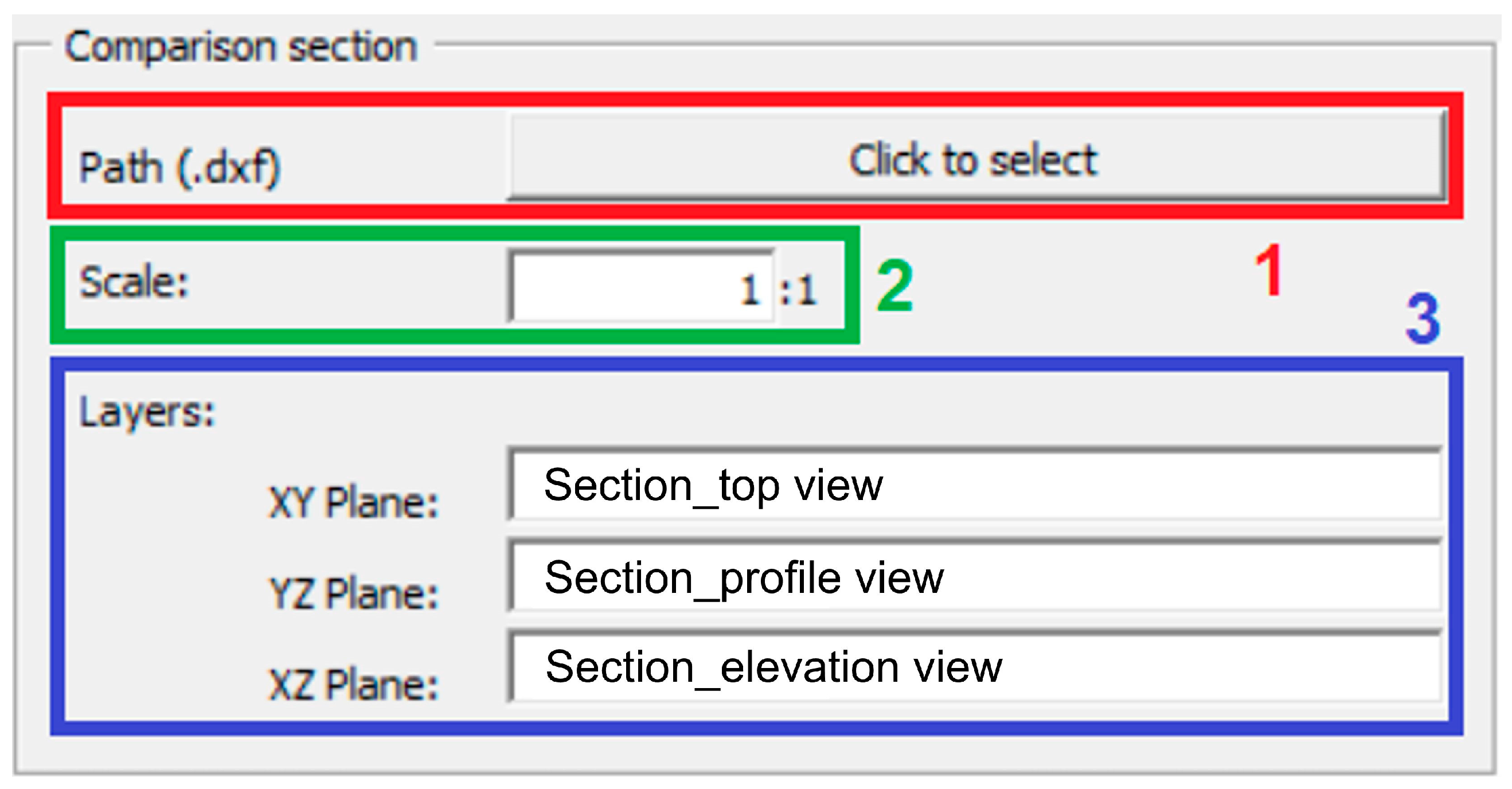
4.1.5. Introduction of Parameters of the Section That Needs to Be Corrected Imported from the External File (‘Comparison Section’ Group)
The steps that one must follow are (
Figure 11):
Path (
Figure 11, Mark 1): The location of the external file in the dxf format, in which the dihedral projections of the section are found, which must be found in a different layer of said file.
Scale (
Figure 11, Mark 2): The scale of the dihedral projections from the external file assuming that the 3D CAD model in CATIA has the real dimensions. Therefore, this is the relationship between the dimensions of the section that needs to be corrected (external file) and the dimensions of that which was obtained by CATIA, whereby only the first number of the scale (i.e., magnification scale) can be changed. The default value of this relation is one, that is, both of the dihedral projections have the same dimensions.
Layers (
Figure 11, Mark 3): The names of the layers that contain the dihedral projections of the section in the external file are identified, for which it is important to locate each layer with the plane to which it corresponds in the dihedral projections obtained in CATIA. By default, three explanatory names appear, but they do not impose the ordering of the layers.
4.1.6. Macro Execution
To start the execution of the macro, it is necessary to press the ‘Start_SectionCheck’ button, which is located in the lower right -hand -side part of the interface. As previously mentioned, depending on the number of lines and the precision selected, the execution time varies considerably.
4.2. Analysis of Results
The results obtained can be divided into graphic and numeric ones. In the former one, the superimposed sections are presented in CATIA for visual comparison, while the latter ones are presented as data in the spreadsheet, together with the calculations of the observed errors.
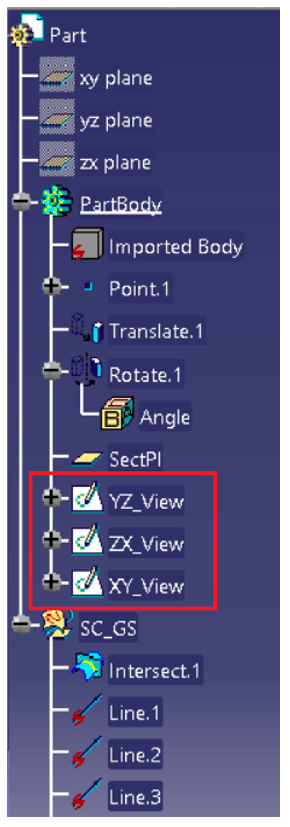
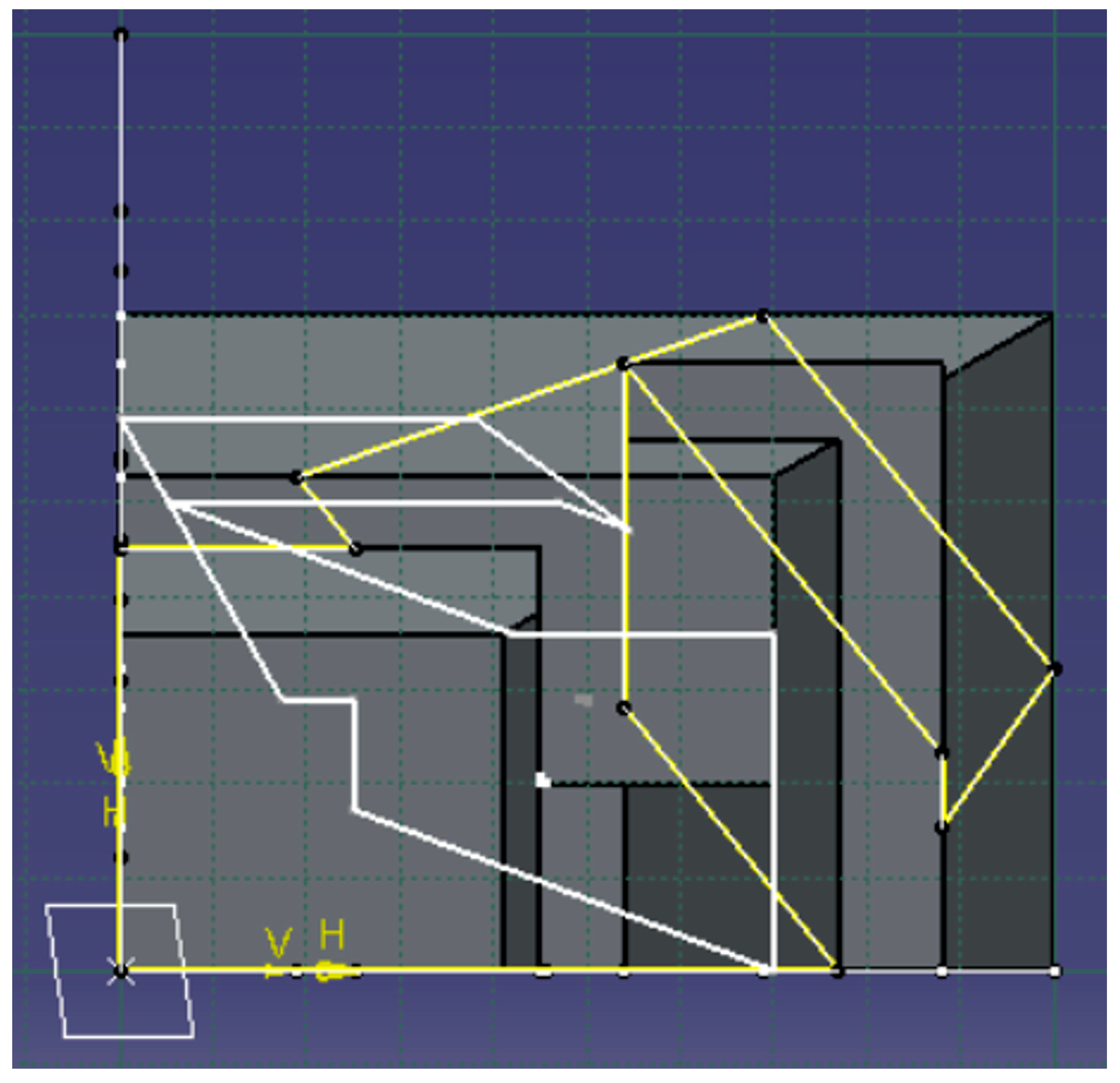
4.2.1. Graphical Results
The graphic results are the representations of the three dihedral projections of each section. To facilitate their comparison, each of the projections of the reference section in CATIA are represented jointly with the corresponding projections of the section that needs to be corrected. To this end, the
Sketches of each of the projection planes in CATIA are used. Their location in the operations tree is shown in red (
Figure 12).
These results are largely indicative and facilitate the reading of the numerical data. There are no error identifiers herein since the analysis is purely visual. However, this representation is especially useful for detecting errors in the data entry, for example, in scaling or placing the layers on the correct coordinate plane.
Figure 13 and
Figure 14 show such examples.
4.2.2. Numerical Results
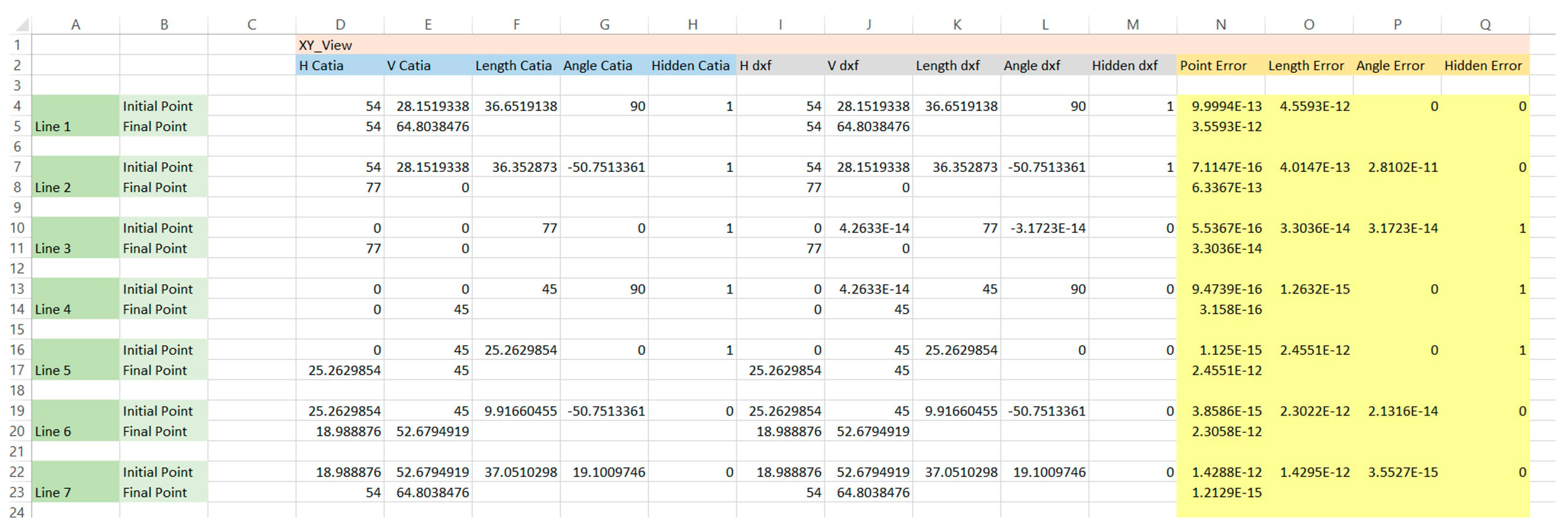
The numerical results include various items of data and errors related to each of the lines that form the projections of the section, and they are represented in a spreadsheet that opens automatically when the macro is executed. Said spreadsheet is created from scratch, and it is not closed when the execution of the macro is finished, and hence, it is available to the user to perform any type of modification or additional calculation to those carried out automatically in the application. Finally, the application features the option to save the numerical results.
The structure of the spreadsheet (
Figure 15) is divided as explained below.
The various lines that make up each dihedral projection of the section are placed in the rows, using two rows for each line, one for each end point of said line. However, there may be a different number of lines in different dihedral projections due to the possible existence of lines that are perpendicular to a dihedral projection or because a line may have different visibility changes in each view. As can be seen, all of the data and errors for all the lines are represented individually.
Likewise, in the columns, several divisions into blocks are made:
Projections: The first division corresponds to the dihedral projection to which the data refers. Three blocks correspond to this division, one for each of the projection planes that are employed (XY, YZ, and XZ).
Types of data: the next level of divisions refers to the application of the data.
- ○
Reference section data: data are obtained from the section generated by CATIA, either through direct measurements or data obtained after manipulating these measurements.
- ○
Data of the section that need to be corrected: the data are stored in the dxf file or calculated from this stored data.
- ○
Errors: comparisons of the previous data are performed.
Values or data: for each aforementioned group, four different numerical values are represented.
- ○
Point coordinates: Both for the CATIA data and for the dxf file, the coordinates are presented separated into two columns, one is for the horizontal coordinate and the other one is for the vertical coordinate according to the plane. In the case of errors, these data are unified in a single comparison that combines the two coordinates of the corresponding point. Furthermore, since both of the points are taken into account, the error in the coordinates of the point unifies the four values located in the same row.
- ○
Longitude: this is calculated from the coordinates of the points of the longitude of the line or from the relative error in this parameter.
- ○
Angle: like the length, this is a calculation that is performed using the coordinates, and it represents the angle that the line forms with respect to the horizontal plane or the error in said angle between the two lines.
- ○
Hidden: The binary variable represents the hidden lines with a value of one and the visible lines with a value of zero. In the case of an error, it is also a binary variable in which the value of zero implies that the values coincide (absence of error).
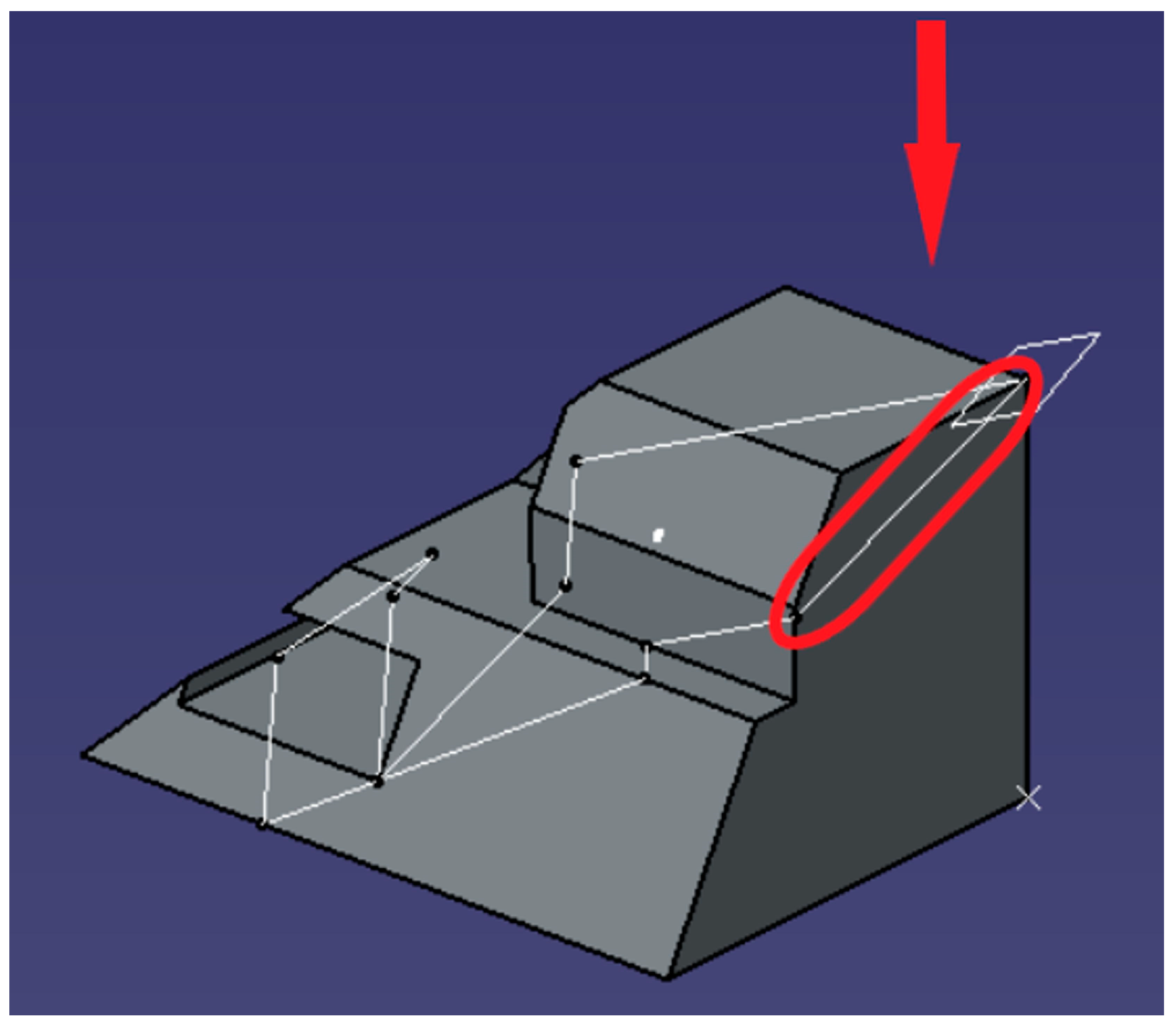
The macro considers the lines on the surfaces parallel to the projection direction to be hidden lines if they do not coincide with its visible edge. Therefore, the highlighted line in the projection marked by the arrow (
Figure 16), whose direction is parallel to the face that contains the line, is represented as a hidden line.
Finally, the global errors are calculated and presented in two rows below the last data series. These results correspond to the arithmetic mean of each type of error, which is carried out on all of the lines of a dihedral projection.
The case of the error in visibility, despite it being calculated in the same way as the other errors are, is a special case since it corresponds to one by its very nature. If all of the lines are wrong, then the error is one in all of them, and the arithmetic mean results in unity. In the opposite case, the result is null. Therefore, the overall result represents the relationship between the number of erroneous lines and the total number of lines.
5. Conclusions
This article presents an application in the field of engineering graphics, which corrects the sections of a plane for a part by comparing the solution provided by the student with that obtained through 3D CAD software. This application has been generated as a CATIA macro that was written in the Visual Basic for Applications (VBA) language, which could be very useful from an educational point of view in university teaching and, in fact, it was designed to be utilized as an assessment resource in the first year of university engineering studies.
The macro allows the user to enter the input data in a very simple and comfortable way, and its execution can be performed by simply pressing a button without having to enter the CATIA macro menu. For the output of the results, the CATIA ‘Sketcher’ option has been employed due to its format of a set of two-dimensional elements, along with the Microsoft Excel spreadsheet for its ease in displaying a large number of numerical values.
Visual Basic for Applications (VBA) has an internal CATIA editor that enables the macro to be ordered and viewed simply. Furthermore, the window creation system (UserForms) simplifies their design considerably, and its possible modification through codes allows adaptations to be made during the execution of the macro. Lastly, communication with Microsoft Excel is direct, which represents an advantage in the export of data and partly explains the use of this software.
Likewise, by considering the large number of operations carried out by the macro to obtain the numerical results and to represent both of the sections correctly, it can be estimated that the time taken by a student to carry out all of this work without the help of the application greatly exceeds that which is needed by the macro, thereby justifying its use.
The following points are proposed as future developments and improvements:
The expansion of the range of possible geometries, including the parts with curved surfaces.
The optimization of the visibility function, since it requires a relatively long execution time if results of high precision are pursued.
The extension to include other methods for the selection of the external geometry (section that needs to be corrected), for example, through other formats other than the dxf format.
Improvement to the information that the user receives during the execution of the application, such as a more exhaustive detection of errors.


 ,
, 


