Design and Development of a Geometric Calculator in CATIA

Abstract

In this article, an application in the field of engineering graphics is presented for the design of a geometric calculator generated as a macro in CATIA V5. The code of this macro is written in the CATVBA language and utilizes the CATIA internal editor while taking advantage of the capabilities offered by Visual Basic for Applications (VBA). The principal purpose of this application lies in the possibility of creating the three main geometric elements (point, line, and plane) and in solving five types of general geometric problems, and then comparing the results obtained with their equivalent problems from analytical geometry. In particular, within these types of general geometric problems, 34 possible cases are solved: definition of lines (nine cases), definition of planes (12 cases), intersection points (three cases), angles (three cases), and distances (seven cases). These new entities defined with the geometric calculator can serve as support for the generation of new three-dimensional volumes, the creation of auxiliary symmetries, and the dimensioning of various elements. It was verified that the results of the designed macro and the solutions of the analytical equations coincided; therefore, the procedure was validated. Likewise, the module employed herein in the CATIA V5 environment is “Wireframe and Surface Design”, since it enables handling the three basic geometric elements (point, line, and plane), which form the basis of the geometric calculator. Lastly, it is verified how the geometric calculator allows their integration with three-dimensional solids, which represents a notable advance as an aid in its geometric definition.

1. Introduction

Both in the educational and in the professional environment, the importance of understanding engineering graphics techniques holds the key to the performance of the work of an engineer and, therefore, justifies its analysis. Understood as the set of graphic techniques employed to solve engineering problems, they are applied in various fields, such as geographic information systems (GIS) [1,2] and computer-aided design (CAD) [3]. Likewise, other applications have been developed to teach the fundamentals of engineering graphics and geometric loci as tools to help in the engineering design process [4].

In the environment of university education, there are numerous subjects that complement training in engineering graphics, such as descriptive geometry [5], analytical geometry [6], technical drawing [7], and normalization [8]. In particular, geometry, or the branch of mathematics that studies the properties of figures in space, acquires a prominent role in the knowledge that university students must possess and, together with arithmetic, constitutes the oldest part of mathematics [9]. Geometry was already developed in a totally empirical way in ancient Mesopotamia in the second millennium BC, and it is precisely in this period that the principles related to distances, angles, and areas began to be discovered. These principles and their associated formulas were able to be developed mainly due to the needs arising from architecture and astronomy [10]. However, it was not until the time of ancient Greece (499 BC–323 BC) when its study was deepened, with well-known geometers appearing such as Thales of Miletus and Euclid with his famous work “The Elements”, considered to be the most influential book in the history of mathematics [11].

This research has been largely based on the use of analytical geometry, a branch of mathematics that uses algebraic methods and equations for the study of geometric problems such as the study of figures, distances, areas, and points of intersection, as well as the use of descriptive geometry, the branch of mathematics that is responsible for representing three-dimensional objects using projections.

The review of related applications has enabled several examples of software to be found that work with geometric environments. Of these, GEUP 3D [12] stands out the most as a calculation and visualization software in spatial geometry and mathematics that enables the study of figures obtained both analytically and from geometric construction, and that can define and modify fundamental geometric elements such as points, lines, planes, circles, conics, polygons, and polyhedral, as well as operations and calculations on measures and angles. Secondly, Geogebra [13], a free application accessible from any browser, and structured into several modules, among which the graphing and the 3D calculator modules deserve special mention, with the latter showing a three-dimensional Cartesian system together with an interactive keyboard and a library of functions that allow the user to create practically any geometric entity, in addition to performing calculations, transformations, developments, and intersections.

However, these applications do not allow their integration into currently available CAD software; hence, the help that would be provided by working with a geometric calculator within said CAD software for the calculation of various magnitudes or angles is lost when carrying out computer-aided design. Likewise, the concept of a geometric calculator has been the subject of research in other scientific disciplines, such as chemistry [14].

There are numerous examples of computer-aided design and engineering software available today, but CATIA (Computer-Aided Three-Dimensional Interactive Application) is, without a doubt, the most widely used CAD in the field of engineering. For this reason, many universities focus on teaching such software in engineering studies [15]. Likewise, various macros have been developed in the CATIA V5 environment [16,17] that seek to automate processes, using the Visual Basic for Applications (VBA) language, which is the Microsoft Visual Basic macro language utilized for the design of macros in CATIA [18].

Thus, the research presented is completely original and genuinely helps in the 3D design process, since no similar application has been developed in CATIA V5, which underlines the importance of the developed application, since it could increase productivity. Among its different functionalities are the generation of auxiliary elements such as axes of revolution or symmetry, the finding new planes to make projections, and the finding of geometric places with respect to three-dimensional solids.

The remainder of the paper is structured as follows: Section 2 shows the materials and methods used in this investigation. Section 3 presents the main results and discussion, while Section 4 states the principal conclusions and future developments.

2. Materials and Methods

2.1. CATIA and VBA

As occurs in most CAD software, CATIA allows the creation of different solids following a procedure that consists of making a two-dimensional sketch, using points, lines, planes, and curves, to which various functions can be applied for its transformation into a three-dimensional solid. Subsequently, other transformations can be applied to said three-dimensional solid, or solids can be combined with each other through Boolean logic operations (union, difference, and intersection).

CATIA presents a variety of modules for the execution of different operations. Of these, “Wireframe and Surface Design” stands out, which is oriented toward the generation of surfaces and is essential for the objective of this research, since it enables basic elements of geometry, such as points, lines, and planes, to be handled.

Likewise, in its V5 version, CATIA includes the possibility of adding new functionalities through a macro programming module in VBA. Visual Basic for Applications is a macro programming language that enables the addition of functionality to Windows-based programs. In turn, a macro is a sequence of orders or commands that are executed automatically to save the user time and work.

Within said programming module, one interesting option included in CATIA (and most software with VBA) is that of the macro recorder. When this tool is activated, macro codes are generated automatically, which replicate the actions carried out by the user himself. This tool creates a file that can be saved in the macro library to be employed on other occasions, thereby obviating the need of the user to iteratively carry out the actions that have already been recorded. Furthermore, CATIA includes a Visual Basic editor that enables existing codes to be changed, as well as the manual creation of macros.

It is interesting to note that the interaction between the end user and the macro is carried out through forms, which are nothing more than text boxes that allow the user to select options, enter values, and receive different outputs from the program.

In the particular case of the application developed herein, a shortcut icon has been placed in the toolbar of the “Wireframe and Surface Design” module (Figure 1) to access the geometric calculator, although it can also be accessed by selecting from the “Tools” tab of the program menu bar and taking the “Macros” option.

2.2. Geometric Calculator

The developed macro consists of two independent modules, with 14 forms and 38 different functions, which follow the hierarchy shown in the flowchart (Figure 2).

In said flowchart, both modules are clearly differentiated: in Module 1, the geometric elements (points, lines, and planes) are generated; in Module 2, the five types of geometric problems posed are solved (find the point of intersection, define a line or a plane, and determine angles and distances).

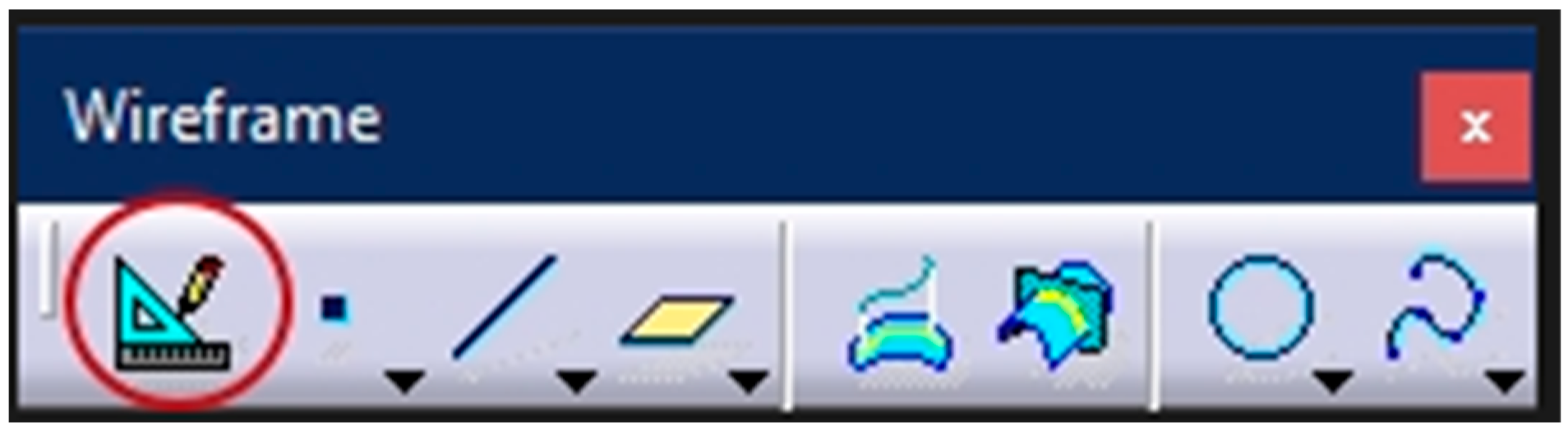
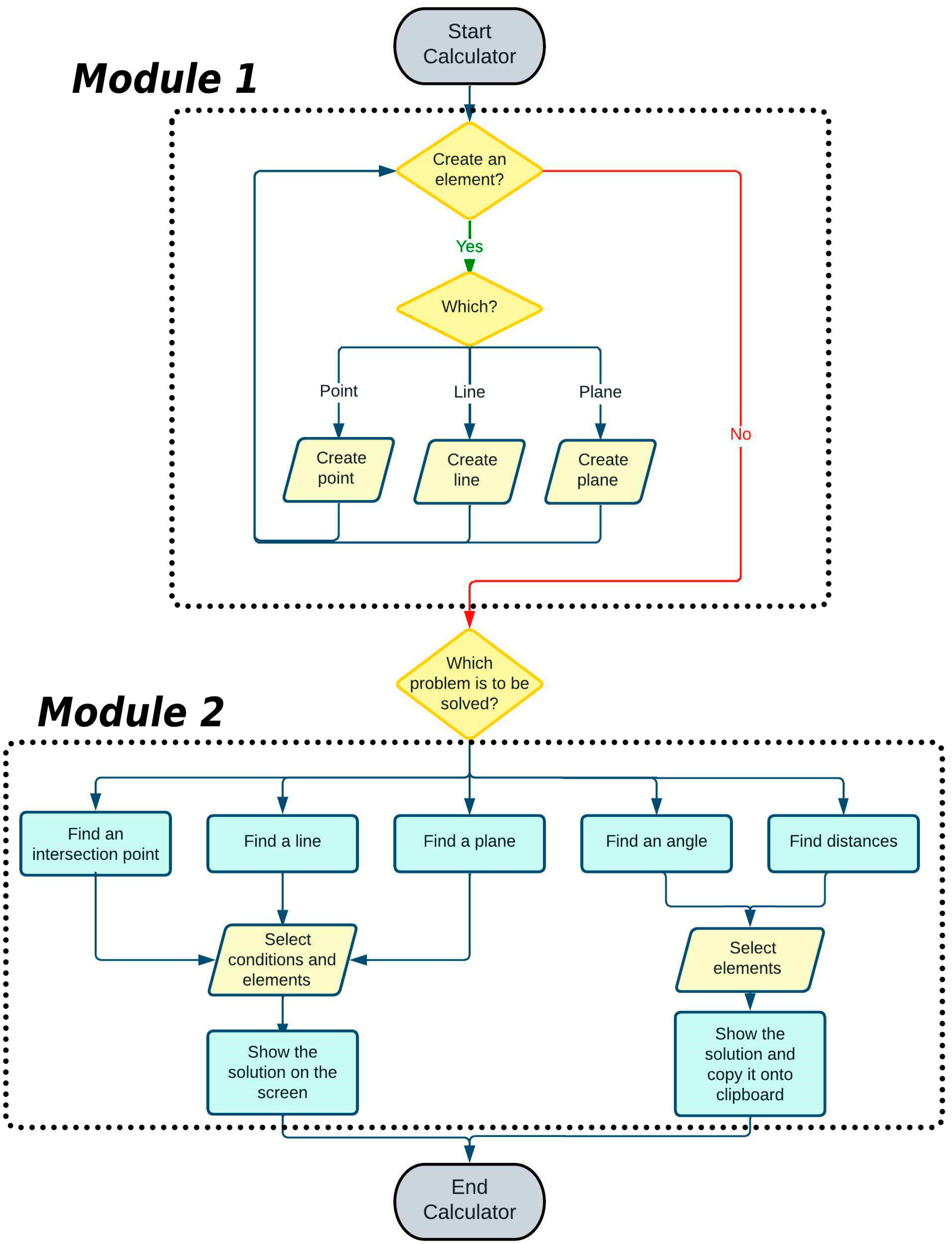
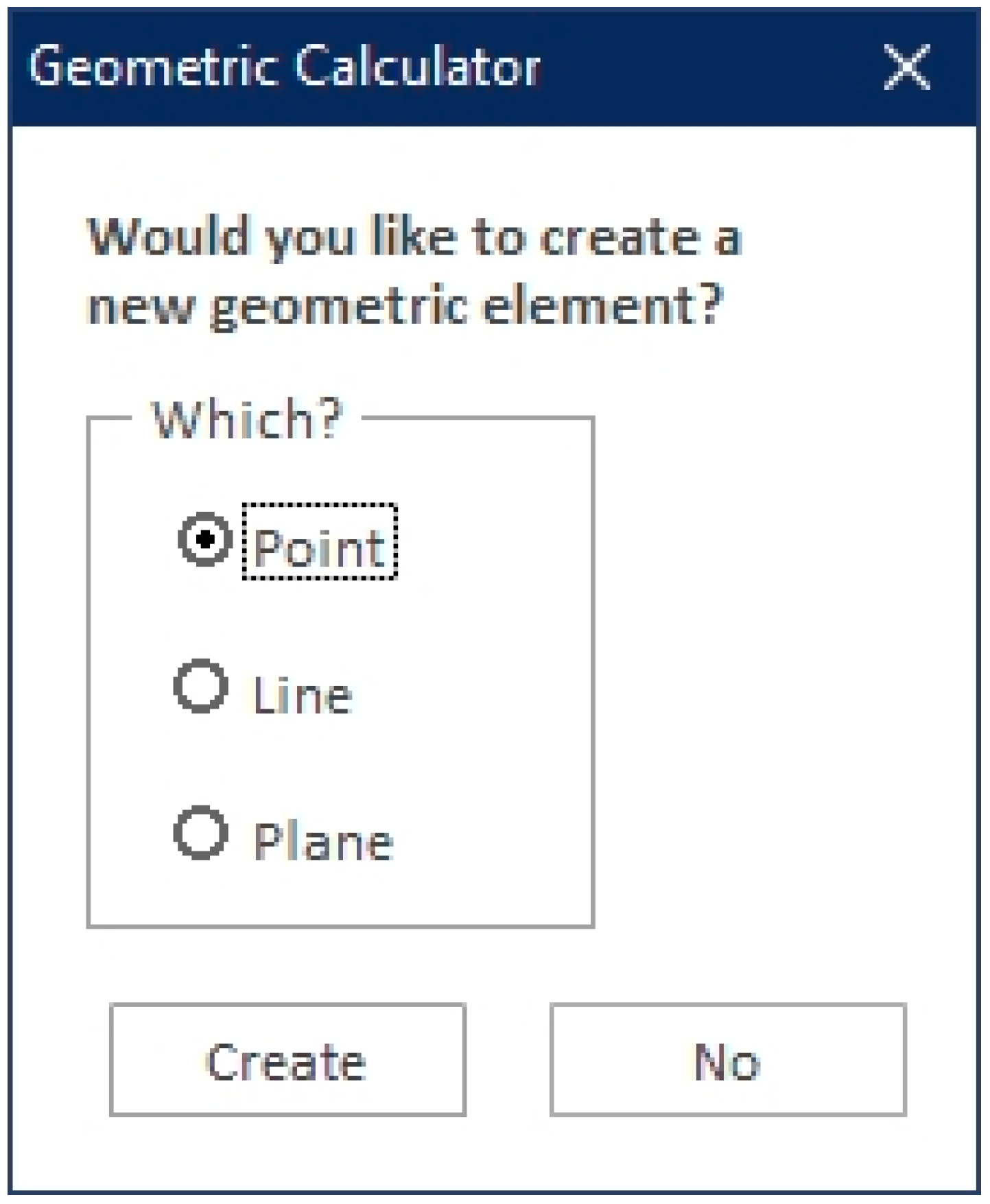
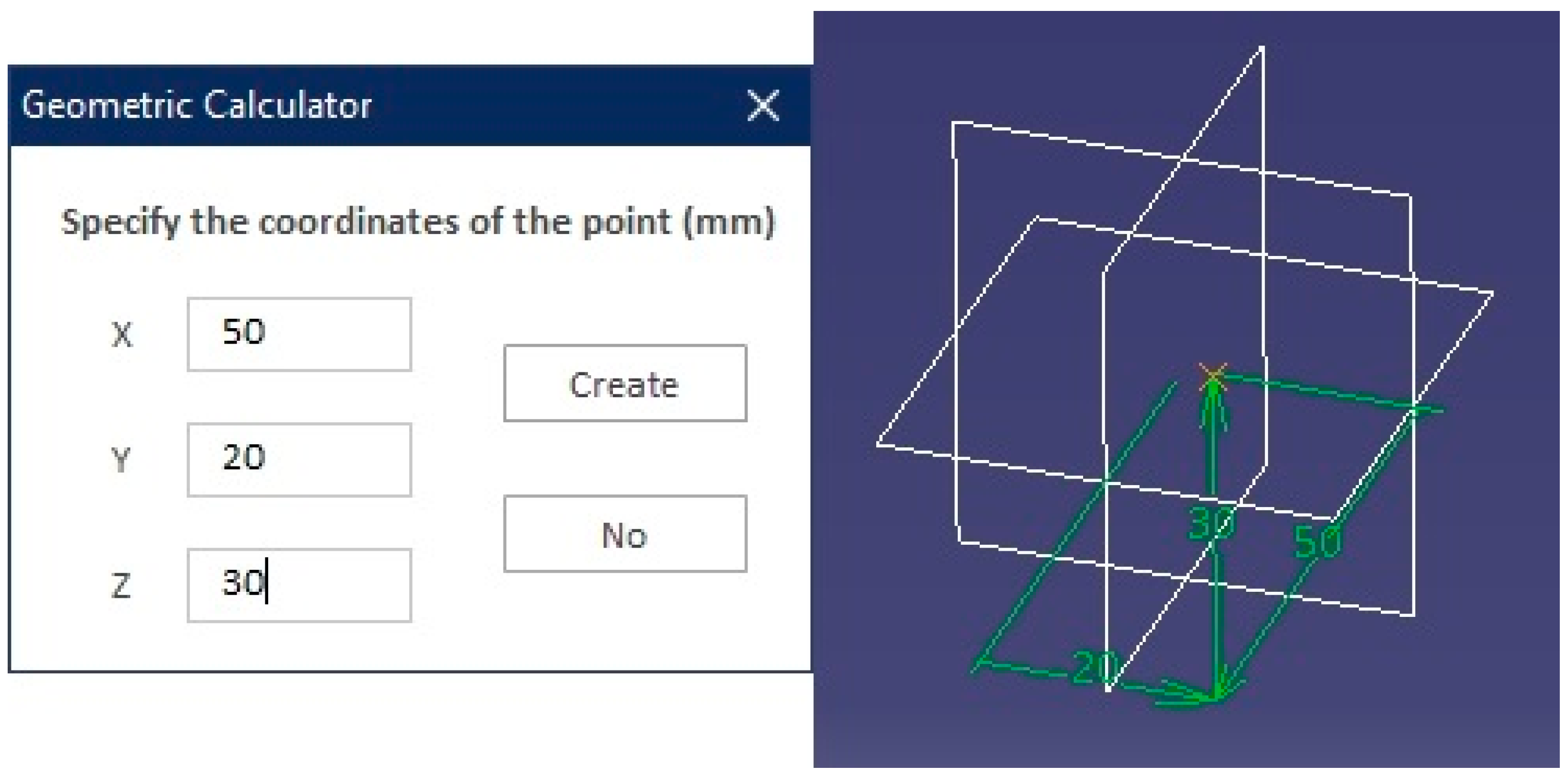
2.2.1. Module 1: Generation of Geometric Elements

The objective of this first phase is to create the entities (geometric elements) with which the geometric calculator will work. First, the user is asked if they want to generate points, lines, or planes (Figure 3).

Thus, depending on the user’s choice, several situations can occur:

• If the option to create a point is chosen, then its Cartesian coordinates (X, Y, Z) must be entered (Figure 4, left), and the geometric calculator will generate it automatically (Figure 4, right).

To store the coordinates entered by the user, the following code is used:

Sub CreateButton_Click()

If “Create” is pressed, then the values are saved and the function CreatePoint is called

X = TextBox1.Value

Y = TextBox2.Value

Z = TextBox3.Value

Call CreatePoint(X,Y,Z)

End Sub

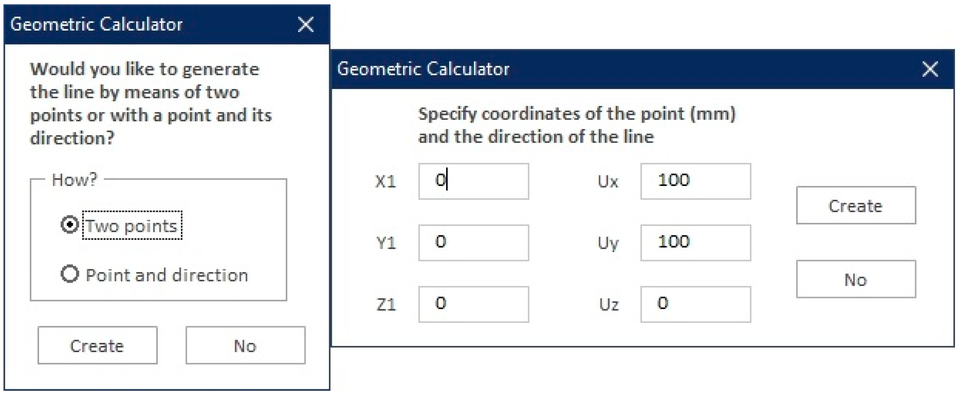
• If the creation of a line is selected (Figure 5, left) a form appears where the user must choose between creating it either depending on two points or with one point and the direction vector of said line (Figure 5, right). The code for the two cases is the same; in the case that a point and the direction of the line are specified, then the program calculates a second point of the line automatically:

Sub CreateButton_Click()

If “Create” is pressed, then the values are saved and the CreateLine function is called

X1 = TextBox1.Value

Y1 = TextBox2.Value

Z1 = TextBox3.Value

X2 = CDbl(TextBox1.Value) + CDbl(TextBox4.Value)

Y2 = CDbl(TextBox2.Value) + CDbl(TextBox5.Value)

Z2= CDbl(TextBox3.Value) + CDbl(TextBox6.Value)

Call CreateLine(X1,Y1,Z1,X2,Y2,Z2)

End Sub

• If the creation of a plane is selected (Figure 6, left), then the Cartesian coordinates of three nonaligned points or the four coefficients (A, B, C, and D) of the general equation of the desired plane (Figure 6, right) are selected:

Ax + By + Cz = D

(1)

Once the values entered for the four coefficients have been accepted, the program generates a plane according to the following code:

Sub CreateButton_Click()

If “Create” is selected, then the values are saved and the CreatePlane function is called

A = TextBox1.Value

B = TextBox2.Value

C = TextBox3.Value

D = TextBox4.Value

Call CreatePlane(A,B,C,D)

End Sub

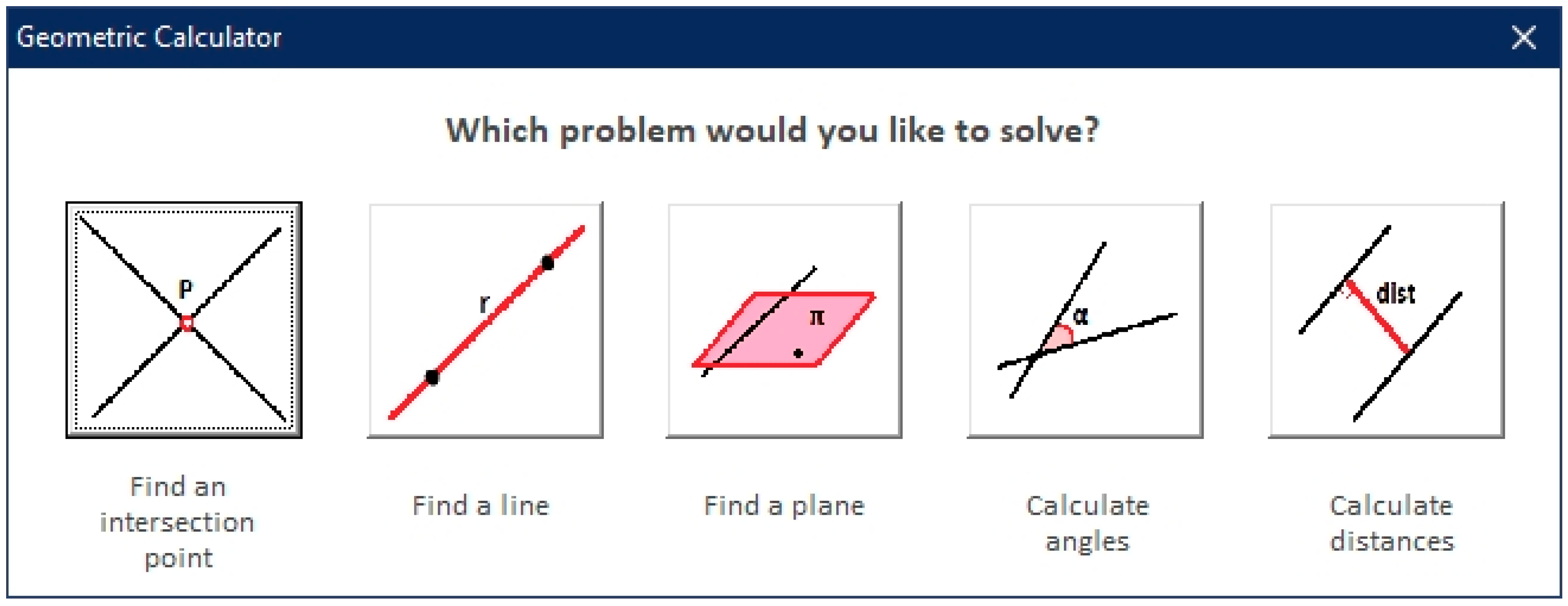
2.2.2. Module 2: Geometric Calculator

This module solves geometric problems of various types, and asks the user first which type of problem is to be solved from among the five options available:

• Find the point of intersection between lines and/or planes.
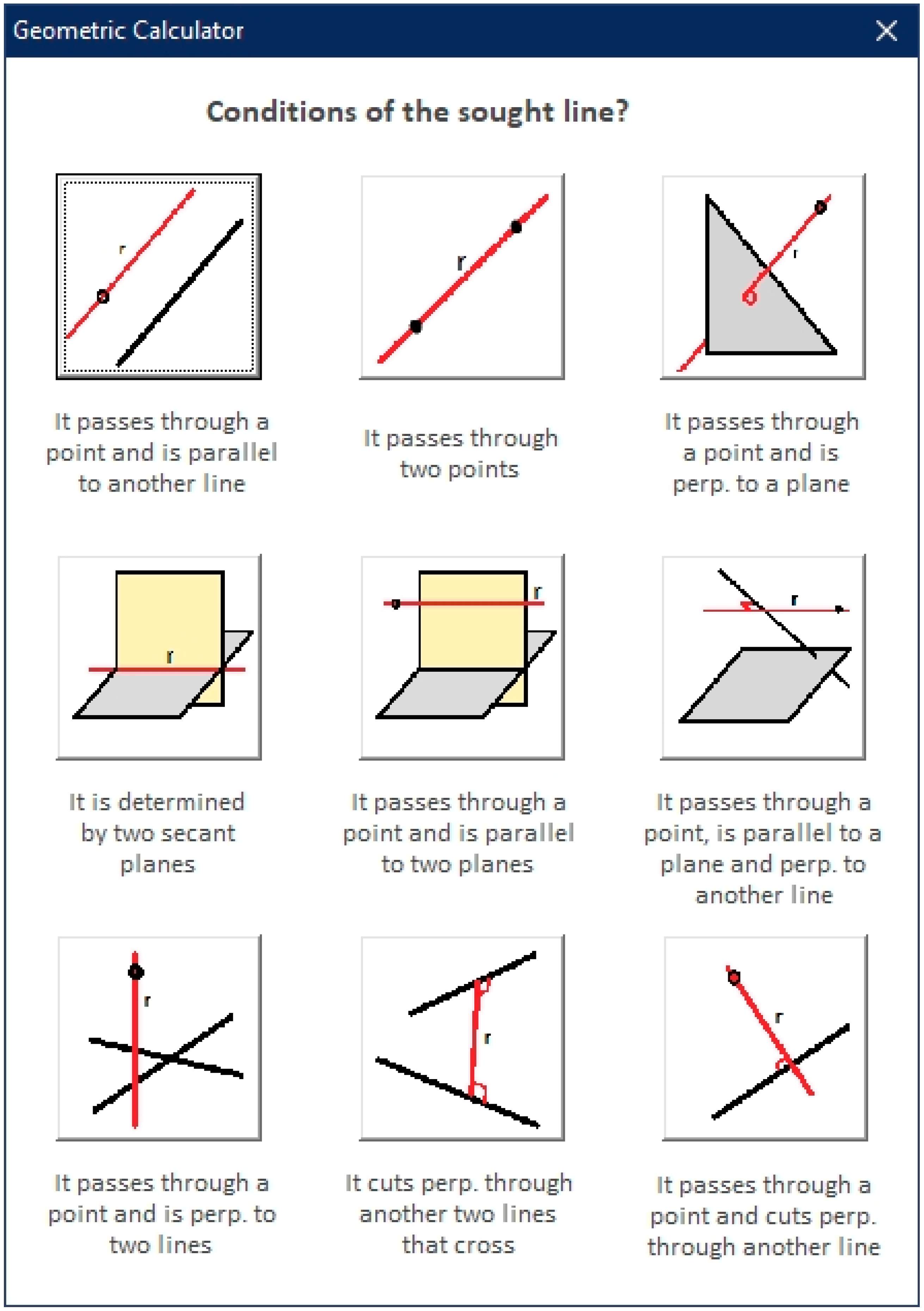
• Define a line that meets certain conditions.
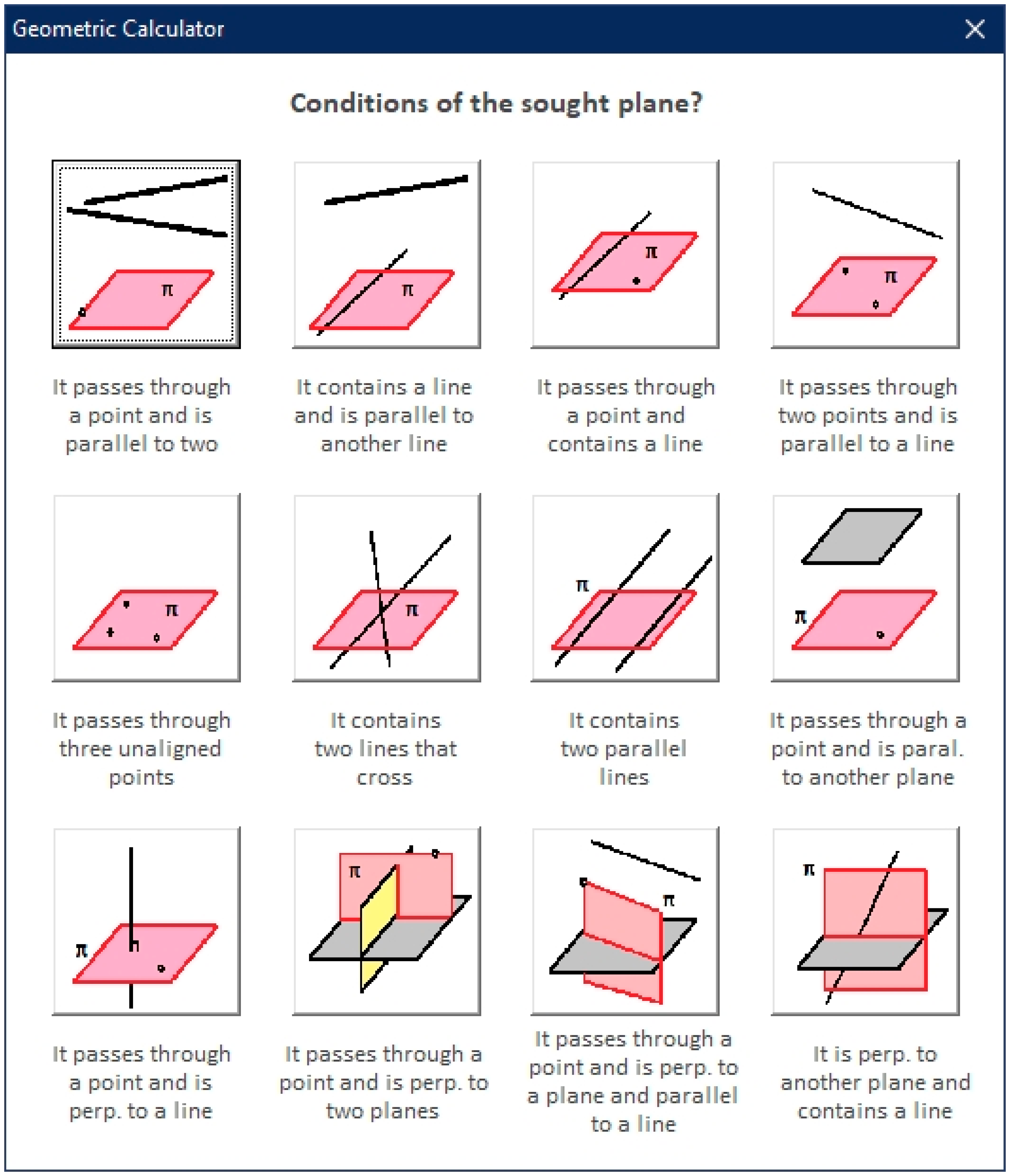
• Define a plane that meets certain conditions.
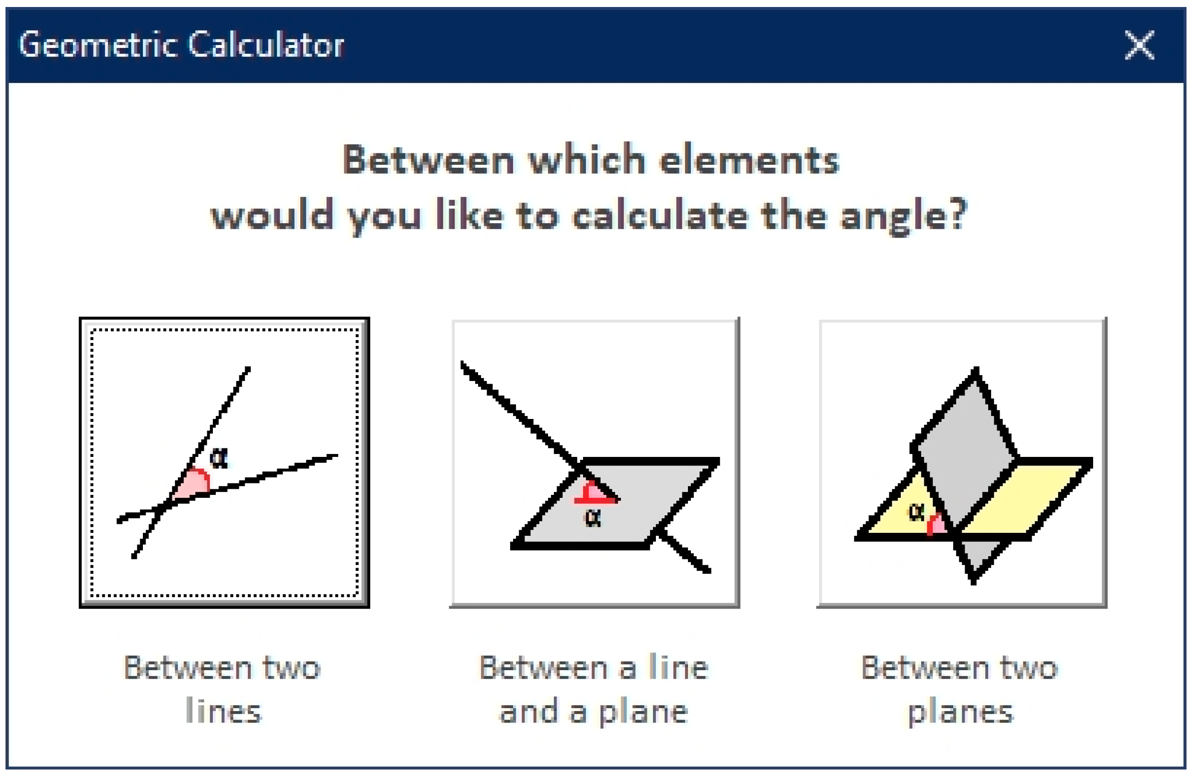
• Calculate the angle between lines and/or planes.
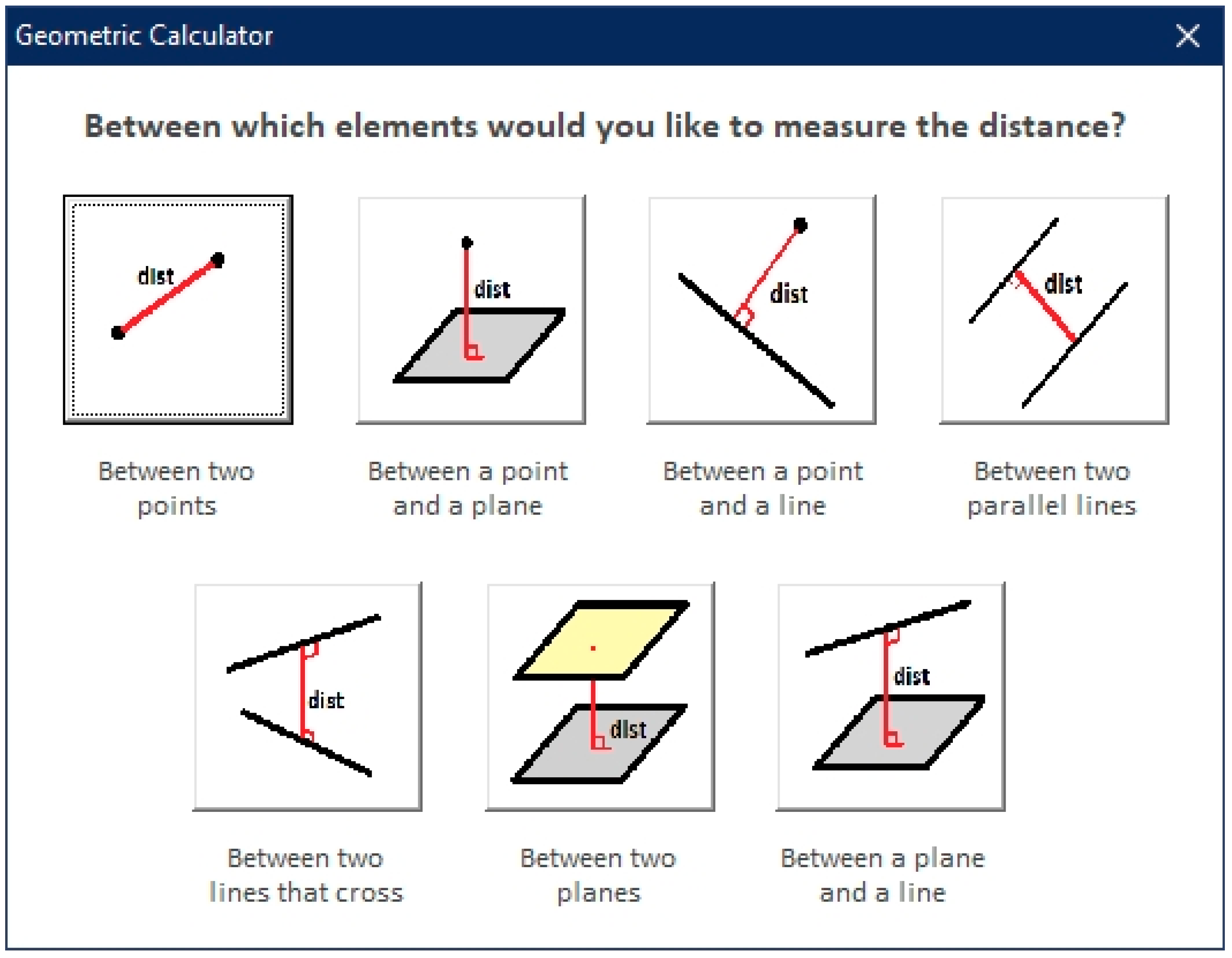
• Calculate the distance between points, lines, and planes.

Figure 7 shows the main form of Module 2 (geometric calculator) where the option buttons of Module 1 have been replaced by command buttons with integrated images since they are more intuitive. These buttons lead the user to the appropriate form with the corresponding subsections.

By pressing any of the five available buttons, which refer to each type of problem, a new menu opens with the subsections corresponding to each specific geometric problem. Each of the five buttons is assigned a name, and they are programmed with the following code to automatically open the corresponding form:

Private Sub Point_Click()

UF_Calculator.Hide

UF_ProblemPoint.Show

End Sub

Private Sub Line_Click()

UF_Calculator.Hide

UF_LineProblem.Show

End Sub

Private Sub Plane_Click()

UF_Calculator.Hide

UF_PlaneProblem.Show

End Sub

Private Sub Angle_Click()

UF_Calculator.Hide

UF_AngleProblem.Show

End Sub

Private Sub Distance_Click()

UF_Calculator.Hide

UF_ProblemDistance.Show

End Sub

To solve each specific geometric problem, the CATIA commands outlined in

Table 1. Commands used for solving geometric problems.

Type of Problem	Commands
Intersection point	AddNewIntersection
Line	AddNewLinePtDir AddNewLinePtPt AddNewLineNormal AddNewLineAngle AddNewIntersection AddNewPlaneAngle AddNewPlane2Lines
Plane	AddNewPlaneNormal AddNewPlaneAngle AddNewPlane1Line1Pt AddNewPlane2Lines AddNewPlane3Points AddNewPlaneOffsetPt AddNewLinePtPt AddNewIntersection
Angle	GetAngleBetween
Distance	GetMinimumDistance

are used.

Find Point of Intersection

In this case, the point of intersection between two intersecting lines, between a line and a plane that are not parallel, or between three nonparallel planes (Figure 8) is addressed. The user must choose which option, and then select the geometric elements requested by the geometric calculator.

Once the geometric elements have been chosen, the calculator finds the intersection point and displays its Cartesian coordinates on the screen using a text box. This is achieved with the execution of the CATIA “Space Analysis” module, which enables dimensions to be used and measurements of the elements of the work environment to be taken. The code used is as follows:

Dim TheMeasurable As Measurable

Dim coords(2)

Dim ref1 As Reference

Set TheMeasurable = TheSPAWorkbench.GetMeasurable(ref1)

TheMeasurable.GetPoint coords

MsgBox “El punto intersección es: (“ & Round(coords(0), 2) & “; “ & Round(coords(1), 2) & “; “ & Round(coords(2), 2) & “) mm”

Dim TheMeasurable As Measurable

Dim coords(2)

Dim ref1 As Reference

Set TheMeasurable = TheSPAWorkbench.GetMeasurable(ref1)

TheMeasurable.GetPoint coords

MsgBox “The intersection point is: (“ & Round(coords(0), 2) & “; “ & Round(coords(1), 2) & “; “ & Round(coords(2), 2) & “) mm”

Find Line

In this option, the user can choose between nine different problems. Each problem finds a straight line that meets certain conditions, such as parallelism, perpendicularity, and location within a plane (Figure 9).

Specifically, the nine problems are a line that passes through a point and is parallel to another line, a line that passes through two points, a line that passes through a point and is perpendicular to a plane, the intersection of two planes, a line that passes through a point and is parallel to two planes, a line that passes through a point is parallel to a plane and perpendicular to a line, a line that passes through a point and is perpendicular to two lines, a line that intersects perpendicular to two crossing lines, and a line that passes through a point and intersects perpendicular to a line.

By choosing one of these options and the necessary geometric elements from the work environment, the new straight line is displayed on the screen. Furthermore, with the GetPointsOnCurve and GetDirection commands, a function capable of generating the equation of the found line has been programmed. This equation is shown on the screen so that the user knows the definition of the generated line.

Likewise, to solve these problems, various automatic methods have been devised on the basis of CATIA’s own options to generate a straight line (point–point, point–direction, angle/normal to curve, tangent to curve, normal to surface, and bisecting), along with other auxiliary commands such as Intersection.

After drawing the desired line on the screen, the geometric calculator presents a text message with its parametric equations, determined with the following code:

Dim TheMeasurable As Measurable

Dim dir(2)

Dim coords(8)

Dim ref1 As Reference

Set TheMeasurable = TheSPAWorkbench.GetMeasurable(ref1)

TheMeasurable.GetDirection dir

TheMeasurable.GetPointsOnCurve coords

MsgBox “The equation of the found line is: “ & vbNewLine & _

“X = “ & Round(coords(3), 2) & “ + t * “ & Round(dir(0), 2) & vbNewLine & _

“Y = “ & Round(coords(4), 2) & “ + t * “ & Round(dir(1), 2) & vbNewLine & _

“Z = “ & Round(coords(5), 2) & “ + t * “ & Round(dir(2), 2)

Find Plane

This third option is the most extensive since it enables a choice among 12 different ways of defining a plane. As in the previous case, the user must impose the conditions for the program to calculate the corresponding plane (Figure 10).

Specifically, the 12 problems are as follows: a plane that passes through a point and is parallel to two lines; a plane that contains a line and is parallel to another; a plane that passes through a point and contains a line; a plane that passes through two points and is parallel to a line; a plane that passes through three non-aligned points; a plane that contains two intersecting lines; a plane that contains two parallel lines, passes through a point and is parallel to another plane; a plane that passes through a point and is perpendicular to a line; a plane that passes through a point and is perpendicular to two planes; a plane that passes through a point is perpendicular to a plane and parallel to a line; a plane that is perpendicular to a plane and contains a line.

Likewise, as in the case of straight lines, these 12 problems are solved using the internal commands that CATIA includes for planes (offset from plane, parallel through point, angle/normal to plane, through three points, through two lines, through a point and line, through planar curve, normal to curve, tangent to surface, equation, and mean through points), and they are adapted to perform the procedure automatically.

A new function has also been programmed that automatically finds the equation of the new plane thanks to the GetPlane command. Thus, at the end of the calculation, the general equation of the found plane is shown, which is obtained as follows:

Dim TheMeasurable As Measurable

Dim coords(8)

Dim A, B, C, D As Double

Dim ref1 As Reference

Set TheMeasurable = TheSPAWorkbench.GetMeasurable(ref1)

TheMeasurable.GetPlane coords

A = coords(4) * coords(8) - coords(5) * coords(7)

B = coords(5) * coords(6) - coords(3) * coords(8)

C = coords(3) * coords(7) - coords(4) * coords(6)

D = A * coords(0) + B * coords(1) + C * coords(2)

MsgBox “The equation of the found plane is: “ & Round(A, 2) & “ * X + “ & Round(B, 2) & “ * Y + “ & Round(C, 2) & “ * Z = “ & Round(D, 2)

Calculate Angles

The geometric calculator allows the calculation of angles between different geometric elements: between two lines (that intersect or cross); between a line and a plane: between two planes (Figure 11).

Likewise, for the calculation of angles, the CATIA “Space Analysis” module is used, dedicated to the study of interferences and intersections and the analysis of measurements and comparisons.

In addition to performing the calculation and displaying the result on the screen, the geometric calculator automatically copies the value obtained to the clipboard for later use.

To this end, the following function has been programmed:

Function CopiarValor(varText As Variant) as String

Dim objCP As Object

Set objCP = CreateObject(“HtmlFile”)

objCP.ParentWindow.ClipboardData.SetData ”text”,varText

End Function

Calculate Distances

The last option available is to calculate distances between the different combinations of geometric elements (Figure 12). Thus, the distance between two points, between a point and a plane, between a point and a line, between two parallel lines, between two crossing lines, between two planes, or between a plane and a line can be evaluated as long as they do not intersect each other, in which case the distance is zero.

As with calculating angles, the geometry calculator saves the measured distance to the clipboard for later use.

3. Results and Discussion

Lastly, in this section, certain geometric problems are solved in order to compare the result of the geometric calculator with that obtained by analytical geometry, thereby verifying the correct functioning of the developed application.

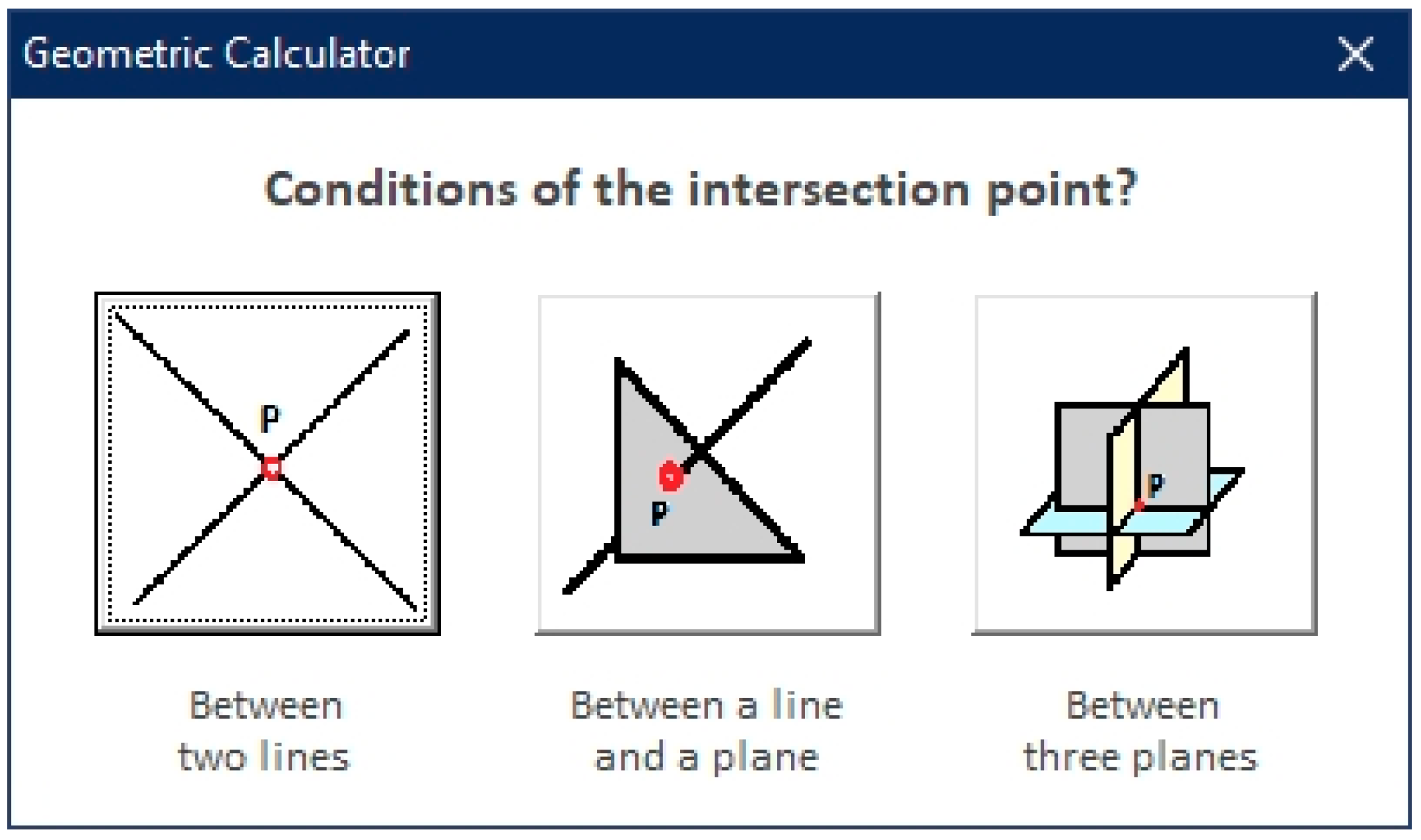
3.1. Calculation of Intersection Point

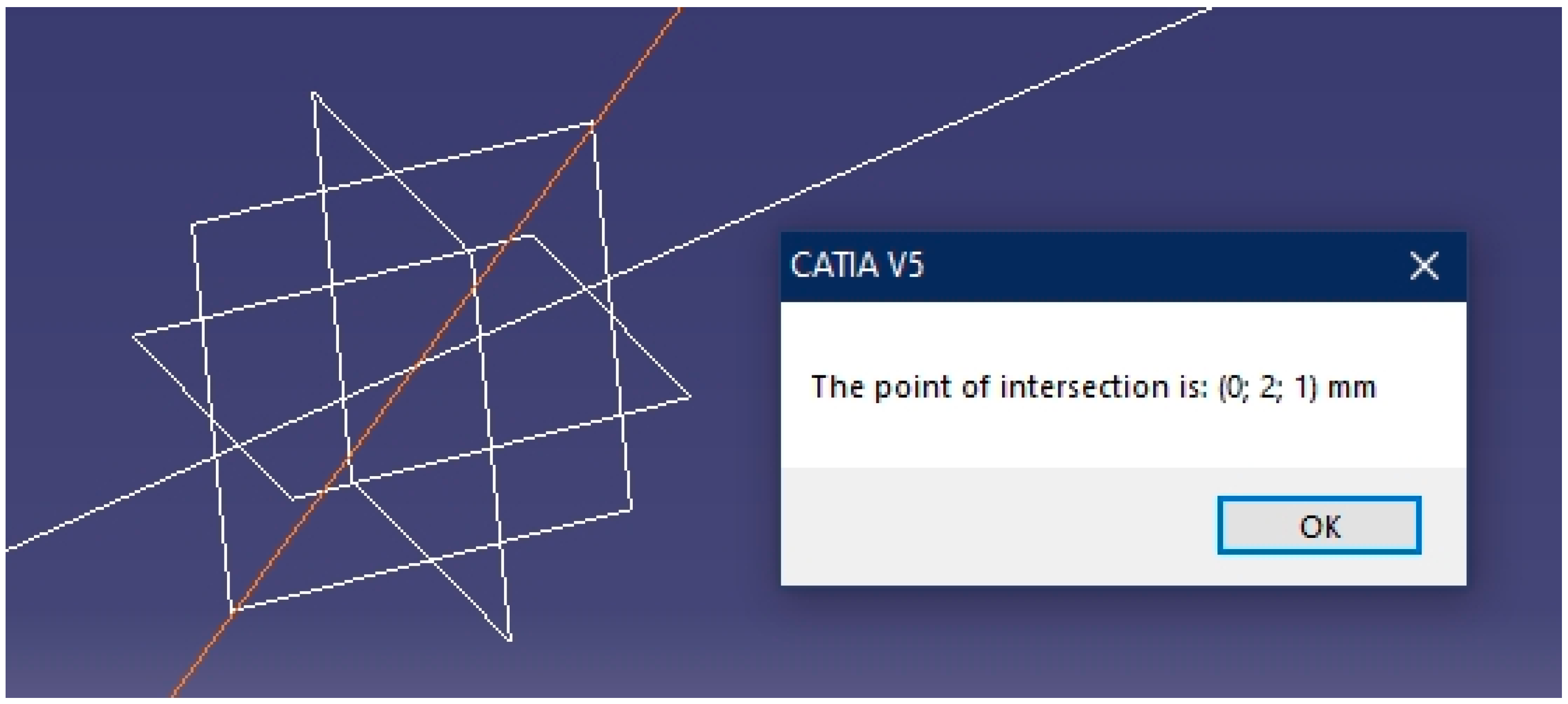
3.1.1. Point of Intersection between Two Lines

In this first case, it is necessary to define two straight lines r and s that intersect, for example:

$$\begin{array}{c}\mathrm{r}\equiv \{\begin{array}{c} \mathrm{x}=3\mathsf{\lambda }\\ \mathrm{y}=2+\mathsf{\lambda }\\ \mathrm{z}=1\end{array}\\ \mathrm{s}\equiv \{\begin{array}{c} \mathrm{x}=1-\mathsf{\mu } \\ \mathrm{y}=2\\ \mathrm{z}=\mathsf{\mu }\end{array}\end{array}$$

(2)

Once these lines are generated in CATIA, the corresponding command button is chosen, and the application returns the result (Figure 13).

To check the result with that obtained by analytical geometry, it is enough to equalize the equations of both lines:

$$\{\begin{array}{c} \mathrm{x}=3\mathsf{\lambda }=1-\mathsf{\mu }\\ \mathrm{y}=2+\mathsf{\lambda }=2\\ \mathrm{z}=1=\mathsf{\mu }\end{array}\to \mathrm{P}\left(0,2,1\right)$$

(3)

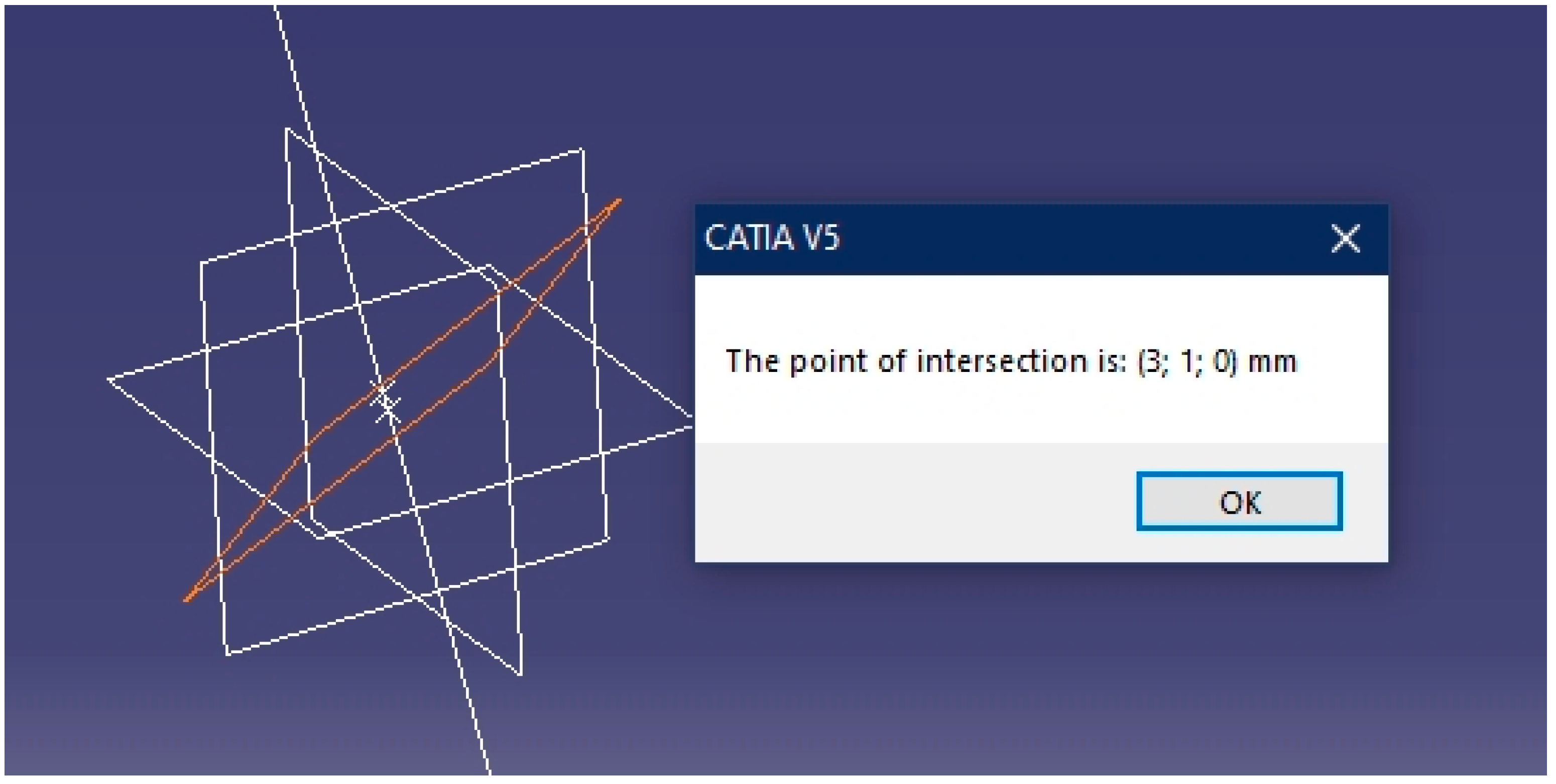
3.1.2. Point of Intersection between a Line and a Plane

For this test, a line r and a plane π are defined randomly, which are not parallel, for example:

$$\begin{array}{c}\mathrm{r}\equiv \{\begin{array}{c}\mathrm{x}=3 \\ \mathrm{y}=1-\mathsf{\lambda }\\ \mathrm{z}=2\mathsf{\lambda }\end{array}\\ \mathsf{\pi }\equiv \mathrm{x}-2\mathrm{y}+2\mathrm{z}-1=0\end{array}$$

(4)

Once created in CATIA, the corresponding option is indicated, and the application returns the result (Figure 14).

In order to verify the analytical solution, the equation of the line is substituted into the equation of the plane and the value of the parameter λ is obtained. Lastly, said value is substituted into the equations of the line, thereby obtaining the coordinates of the point of intersection:

$$\left(3\right)-2\left(1-\mathsf{\lambda }\right)+2\left(2\mathsf{\lambda }\right)-1=0\to \mathsf{\lambda }=0\to \mathrm{P}\left(3,1,0\right)$$

(5)

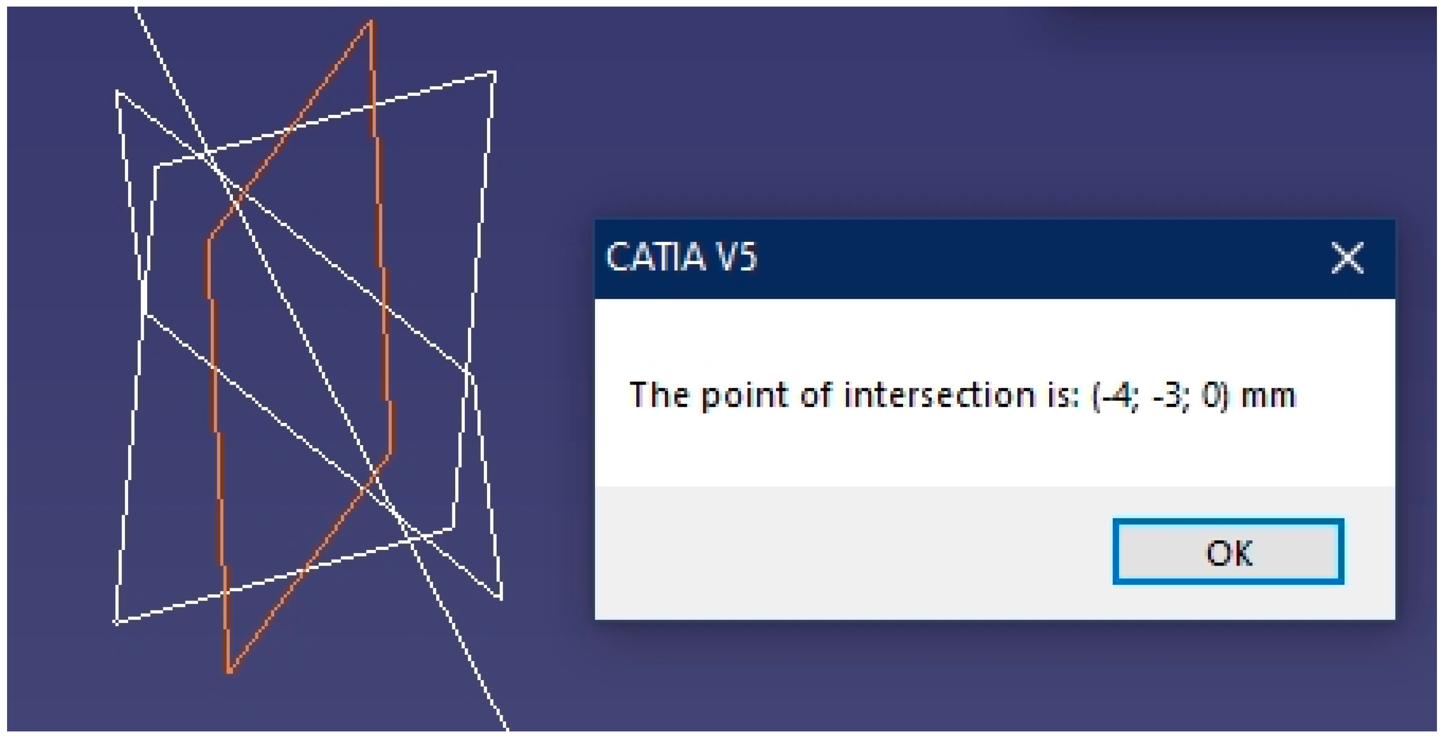
3.1.3. Point of Intersection between Three Planes

For this test, three planes that are not parallel, ${\mathsf{\pi }}_1,{\mathsf{\pi }}_2,\mathrm{and}{\mathsf{\pi }}_3$, are to be defined two by two:

$$\begin{array}{c}{\mathsf{\pi }}_1\equiv 2\mathrm{x}-3\mathrm{y}+4\mathrm{z}-1=0\hfill \\ {\mathsf{\pi }}_2\equiv \mathrm{x}-\mathrm{y}-\mathrm{z}+1=0\hfill \\ {\mathsf{\pi }}_3\equiv -\mathrm{x}+2\mathrm{y}-\mathrm{z}+2=0\hfill \end{array}$$

(6)

Once these planes are generated in CATIA, the corresponding command button is chosen, and the application returns the result (Figure 15).

In order to verify with the analytical solution, the system of three equations with three unknowns that form the three planes is solved, and the point of intersection is obtained:

$$\{\begin{array}{c} 2\mathrm{x}-3\mathrm{y}+4\mathrm{z}-1=0\\ \mathrm{x}-\mathrm{y}-\mathrm{z}+1=0\\ -\mathrm{x}+2\mathrm{y}-\mathrm{z}+2=0\end{array}\to \{ \begin{array}{c} \mathrm{x}=-4\\ \mathrm{y}=-3\\ \mathrm{z}=0\end{array}\to \mathrm{P}\left(-4,-3, 0\right)$$

(7)

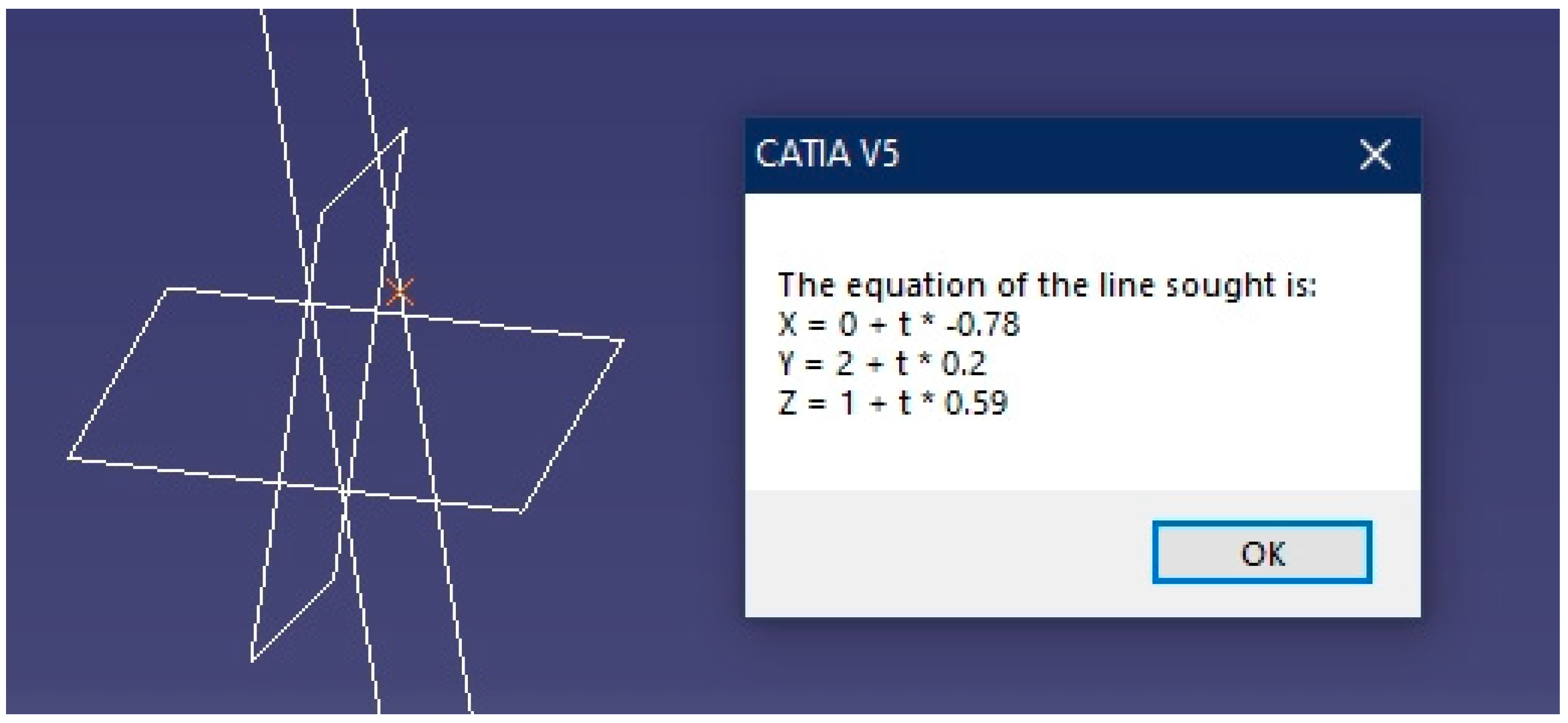
3.2. Determination of Lines

In this second case, and since there are nine geometric problems solved by the geometric calculator, only the resolution of one thereof is shown. In particular, we focus on determining the line that passes through a given point P and is parallel to any two planes ${\mathsf{\pi }}_1\mathrm{and}{\mathsf{\pi }}_2$:

$$\begin{array}{c}\hfill \mathrm{P}\left(0,2,1\right)\hfill \\ {\mathsf{\pi }}_1\equiv \mathrm{x}-2\mathrm{y}+2\mathrm{z}-1=0\hfill \\ {\mathsf{\pi }}_2\equiv \mathrm{x}+\mathrm{y}+\mathrm{z}=0\hfill \end{array}$$

(8)

Thus, once these three geometric elements have been generated in CATIA, the corresponding command button is selected, and the application returns the graphic result and the equation of the sought line (Figure 16).

As verification with the analytical solution, the two normal vectors of the planes (${\overrightarrow{\mathrm{n}}}_1\mathrm{and}{\overrightarrow{\mathrm{n}}}_2$) are multiplied ($\overrightarrow{\mathrm{u}}$) and after normalizing the target vector ($\overrightarrow{{\mathrm{u}}_{\mathrm{n}}}$), with the given point P, the parametric equation of the line is obtained, which coincides with the result obtained by the geometric calculator:

$$\begin{array}{c}\overrightarrow{\mathrm{u}}={\overrightarrow{\mathrm{n}}}_1\times {\overrightarrow{\mathrm{n}}}_2=\left|\begin{array}{ccc}\overrightarrow{\mathrm{i}}& \overrightarrow{\mathrm{j}}& \overrightarrow{\mathrm{k}}\\ 1& -2& 2\\ 1& 1& 1\end{array}\right|=\left(-4,1,3\right)\to \hfill \\ \overrightarrow{{\mathrm{u}}_{\mathrm{n}}}=\frac{\overrightarrow{\mathrm{u}}}{\left|\overrightarrow{\mathrm{u}}\right|}=\frac{\left(-4,1,3\right)}{\sqrt{{\left(-4\right)}^2+1^2+3^2}}=\left(-0.78,0.2,0.59\right)\hfill \\ \hfill \mathrm{r}\equiv \{\begin{array}{c}\mathrm{x}=0-0.78\mathsf{\lambda } \\ \mathrm{y}=2+0.2\mathsf{\lambda }\\ \mathrm{z}=1+0.59\mathsf{\lambda }\end{array}\hfill \end{array}$$

(9)

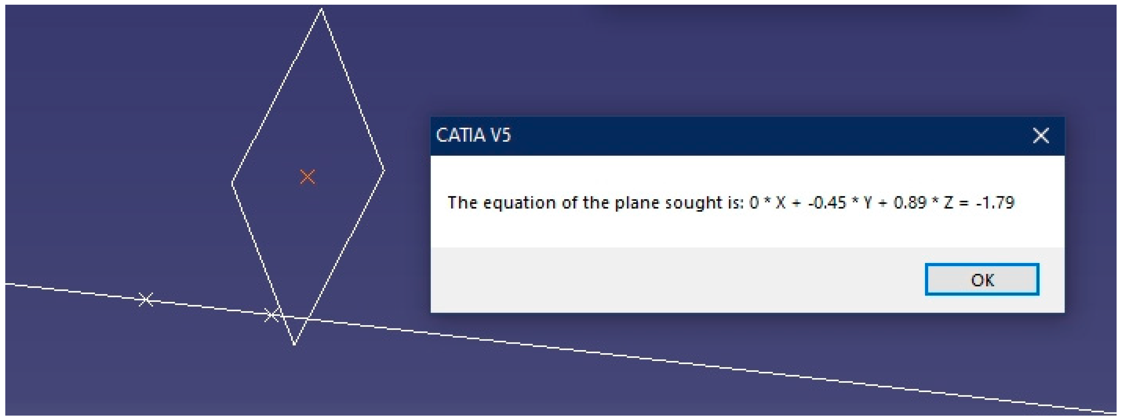
3.3. Determination of Planes

In this third case, since there are 12 geometric problems solved by the geometric calculator, only the resolution of one thereof is shown. Specifically, it was decided to calculate the equation of the plane that is perpendicular to a line and that contains a point. For example, the following point P and line r are known:

$$\begin{array}{c}\mathrm{P}\left(0,2,-1\right)\\ \mathrm{r}\equiv \{\begin{array}{c}\mathrm{x}=3 \\ \mathrm{y}=1-\mathsf{\lambda }\\ \mathrm{z}=2\mathsf{\lambda }\end{array}\end{array}$$

(10)

Thus, once these two geometric elements have been generated in CATIA, the corresponding command button is selected, and the geometric calculator returns the graphic result and the equation of the sought plane (Figure 17).

For verification with the analytical solution, it is obvious that the vector normal to the plane will be the same as the normalized direction vector of the line ($\overrightarrow{{\mathrm{u}}_{\mathrm{n}}}$), since the line and the plane are perpendicular; hence, the equation of the plane is

$$\overrightarrow{{\mathrm{u}}_{\mathrm{n}}}=\frac{\overrightarrow{\mathrm{u}}}{\left|\overrightarrow{\mathrm{u}}\right|}=\frac{\left(0,-1,2\right)}{\sqrt{0^2+{\left(-1\right)}^2+2^2}}=\left(0,-0.45,0.89\right)\to \mathsf{\pi }\equiv 0\mathrm{x}-0.45\mathrm{y}+0.89\mathrm{z}+\mathrm{D}=0$$

(11)

By substituting the point P in Equation (11), the value of the parameter D is calculated; therefore, the equation of the plane is determined:

$$\begin{array}{c}-0.90-0.89+\mathrm{D}=0\to \mathrm{D}=1.79\\ \mathsf{\pi }\equiv -0.45\mathrm{y}+0.89\mathrm{z}+1.79=0\end{array}$$

(12)

3.4. Angle Calculation

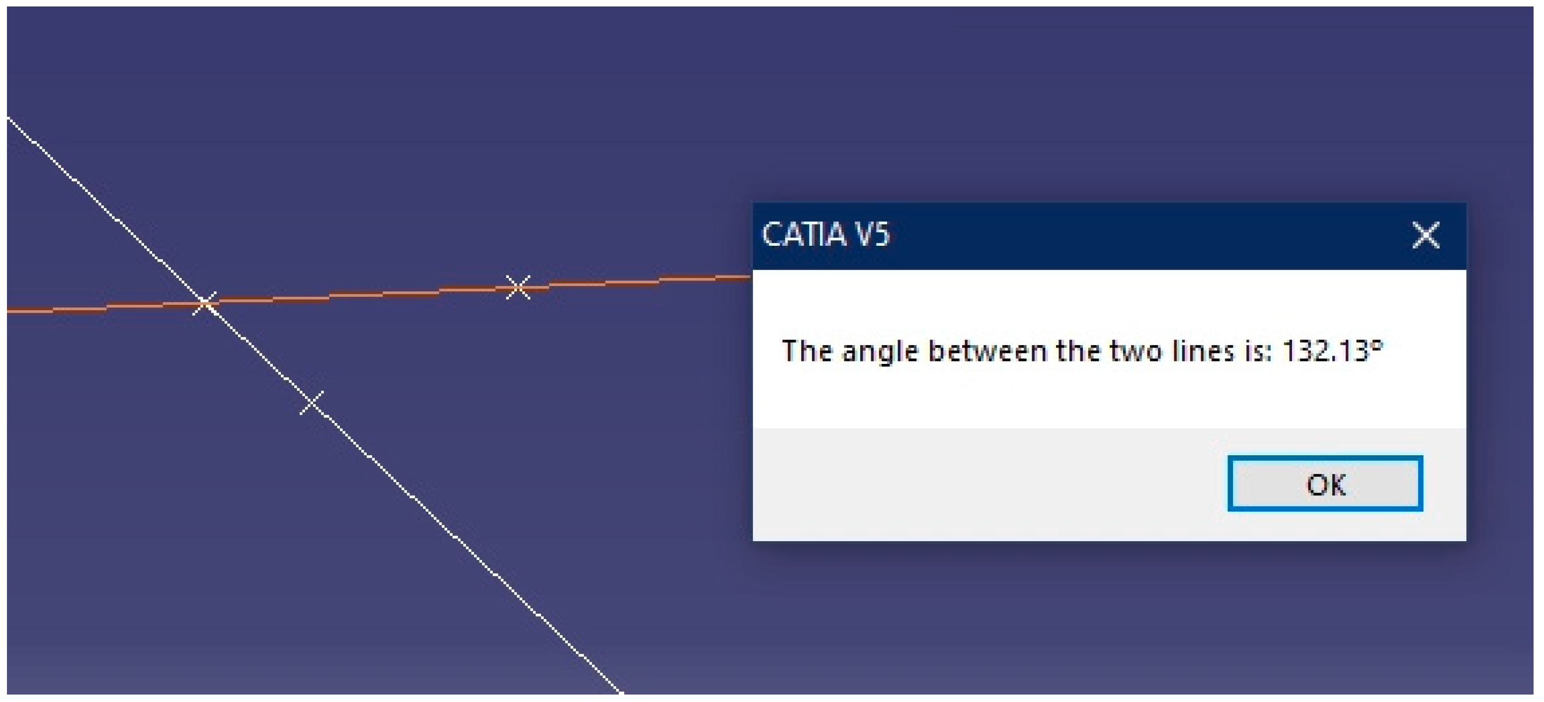
3.4.1. Angle between Two Lines

In this case, the geometric calculator obtains the angle between the two direction vectors of both lines; hence, it provides a solution regardless of whether both lines intersect or not. Given any two lines,

$$\begin{array}{c}\mathrm{r}\equiv \{\begin{array}{c} \mathrm{x}=3\mathsf{\lambda } \\ \mathrm{y}=2+\mathsf{\lambda }\\ \mathrm{z}=1\end{array}\\ \mathrm{s}\equiv \{\begin{array}{c} \mathrm{x}=1-\mathsf{\mu } \\ \mathrm{y}=2\\ \mathrm{z}=\mathsf{\mu }\end{array}\end{array}$$

(13)

Once both lines are defined in CATIA, the geometric calculator returns the graphic result and the angle between them (Figure 18).

To verify the result with that of the analytical solution, it is necessary to employ the scalar product of the direction vectors of both lines (${\overrightarrow{\mathrm{n}}}_1\mathrm{and}{\overrightarrow{\mathrm{n}}}_2$):

$$\begin{array}{c}\cos \left(\mathsf{\alpha }\right)=\frac{{\overrightarrow{\mathrm{n}}}_1·{\overrightarrow{\mathrm{n}}}_2}{\left|{\overrightarrow{\mathrm{n}}}_1\right|·\left|{\overrightarrow{\mathrm{n}}}_2\right|}=\frac{3·\left(-1\right)+1·0+0·1}{\sqrt{3^2+1^2+0^2}·\sqrt{{\left(-1\right)}^2+0^2+1^2}}=\left(\frac{-3}{\sqrt{10}·\sqrt{2}}\right)\to \\ \to \mathsf{\alpha }=\arccos \left(\frac{-3}{\sqrt{20}}\right)=132.13°\end{array}$$

(14)

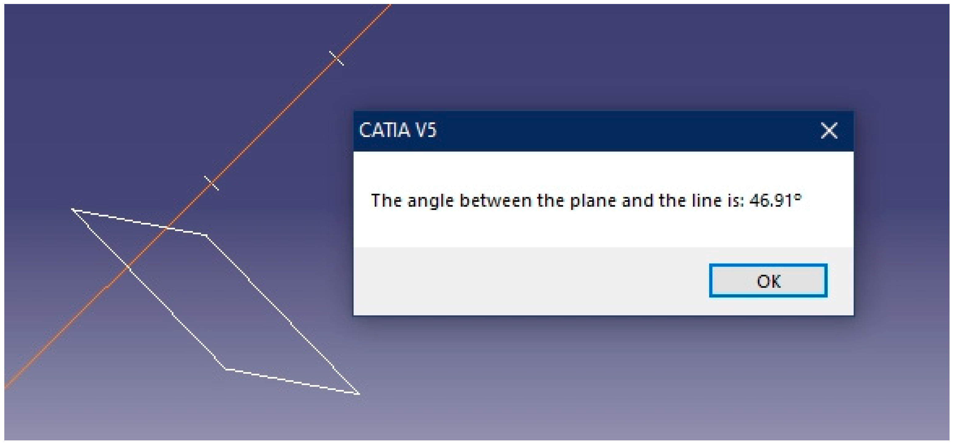
3.4.2. Angle between a Line and a Plane

After randomly defining a line and a plane,

$$\begin{array}{c}\mathrm{r}\equiv \{\begin{array}{c} \mathrm{x}=3\mathsf{\lambda }\\ \mathrm{y}=2+\mathsf{\lambda }\\ \mathrm{z}=1\end{array}\hfill \\ \mathsf{\pi }\equiv \mathrm{x}+\mathrm{y}+\mathrm{z}=0\hfill \end{array}$$

(15)

The geometric calculator returns the graphic result and the angle between the two geometric elements (Figure 19).

As verification with the analytical solution, the angle formed by the direction vector of the line $\overrightarrow{\mathrm{u}}\mathrm{and}\mathrm{the}\mathrm{normal}\mathrm{vector}\mathrm{of}\mathrm{the}\mathrm{plane}\overrightarrow{\mathrm{n}}$, is not the angle formed by the line and the plane ($\mathsf{\beta }$), but its complementary angle ($\mathsf{\alpha }$). By carrying out the relevant operations, the result is attained:

$$\begin{array}{c}\cos \left(\mathsf{\beta }\right)=\frac{\overrightarrow{\mathrm{u}}·\overrightarrow{\mathrm{n}}}{\left|\overrightarrow{\mathrm{u}}\right|·\left|\overrightarrow{\mathrm{n}}\right|}=\frac{3·1+1·1+0·1}{\sqrt{3^2+1^2+0^2}·\sqrt{1^2+1^2+1^2}}=\frac{4}{\sqrt{10}·\sqrt{3}}\to \\ \mathsf{\alpha }=90°-\arccos \left(\frac{4}{\sqrt{30}}\right)=46.91°\end{array}$$

(16)

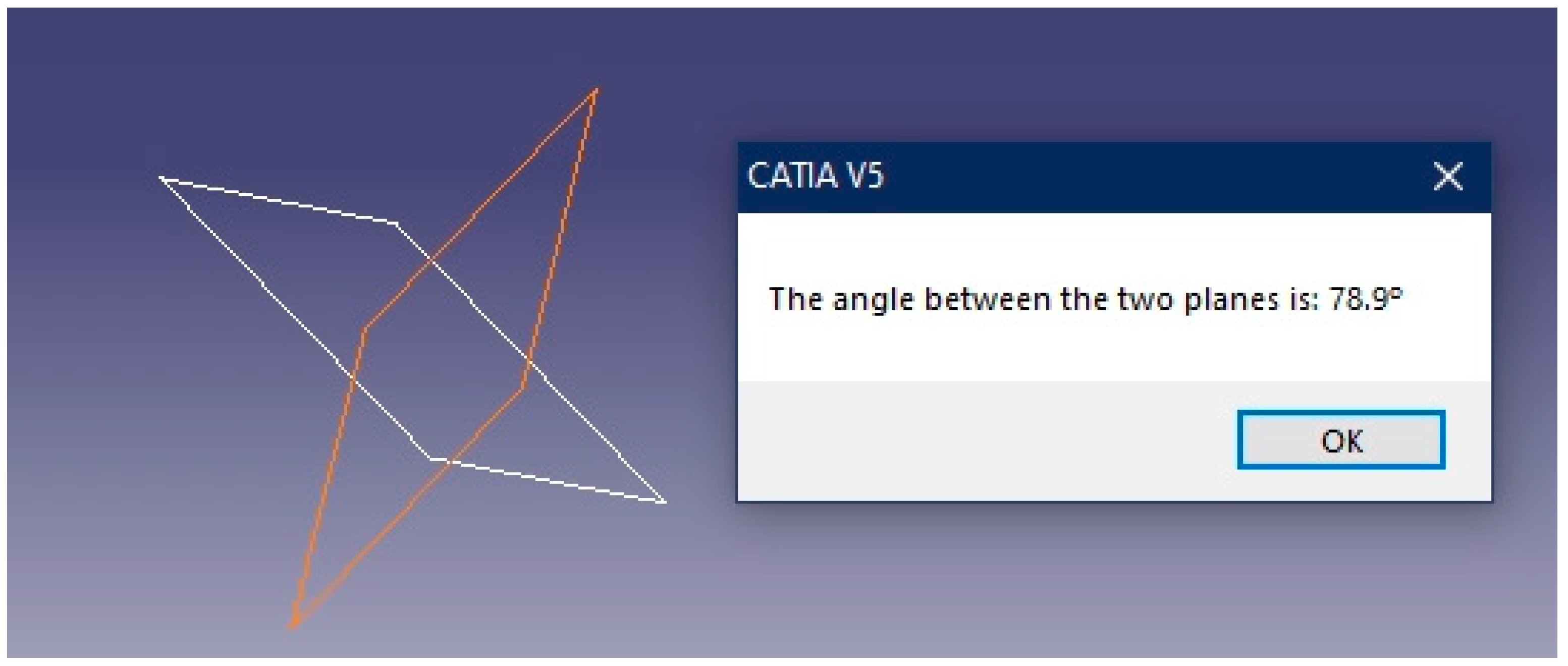
3.4.3. Angle between Two Planes

Likewise, the angle between two planes ${\mathsf{\pi }}_1 \mathrm{and} {\mathsf{\pi }}_2$ can also be measured. For example,

$$\begin{array}{c}{\mathsf{\pi }}_1\equiv \mathrm{x}+\mathrm{y}+\mathrm{z}=0\\ {\mathsf{\pi }}_2\equiv \mathrm{x}-2\mathrm{y}+2\mathrm{z}-1=0\end{array}$$

(17)

Once both planes are defined, and the option of the angle between two planes is selected, the geometric calculator returns the graphic result and the angle between them (Figure 20).

Likewise, as verification, it is known that the angle between two planes is equal to the angle formed by their normal vectors ${\overrightarrow{\mathrm{n}}}_1\mathrm{and}{\overrightarrow{\mathrm{n}}}_2$; therefore, by applying the scalar product,

$$\begin{array}{c}\cos \left(\mathsf{\alpha }\right)=\frac{{\overrightarrow{\mathrm{n}}}_1·{\overrightarrow{\mathrm{n}}}_2}{\left|{\overrightarrow{\mathrm{n}}}_1\right|·\left|{\overrightarrow{\mathrm{n}}}_2\right|}\to \\ \mathsf{\alpha }=\arccos \left(\frac{1.1+1·\left(-2\right)+1.2}{\sqrt{1^2+1^2+1^2}·\sqrt{1^2+2^2+2^2}}\right)=\arccos \left(\frac{1}{\sqrt{3}·\sqrt{9}}\right)=78.9°\end{array}$$

(18)

3.5. Distance Calculation

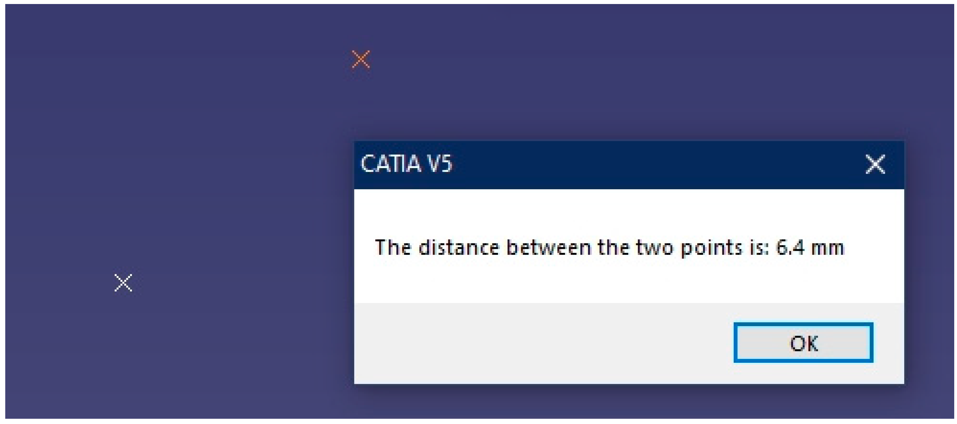
3.5.1. Distance between Two Points

This is the simplest of the seven distance problems implemented in the geometric calculator. Thus, any two points P and Q are defined:

$$\begin{array}{c}\mathrm{P}\left(3,1,0\right)\\ \mathrm{Q}\left(-3,0,2\right)\end{array}$$

(19)

Once both points are defined in CATIA, the geometric calculator returns the result (Figure 21).

As an analytical verification, the distance between the two points is the magnitude of the vector that joins them. Thus,

$$\overrightarrow{\mathrm{PQ}}=\left(-6,-1,2\right)\to |\overrightarrow{\mathrm{PQ}}|=\sqrt{{\left(-6\right)}^2+{\left(-1\right)}^2+2^2}=\sqrt{41}=6.4\mathrm{units}$$

(20)

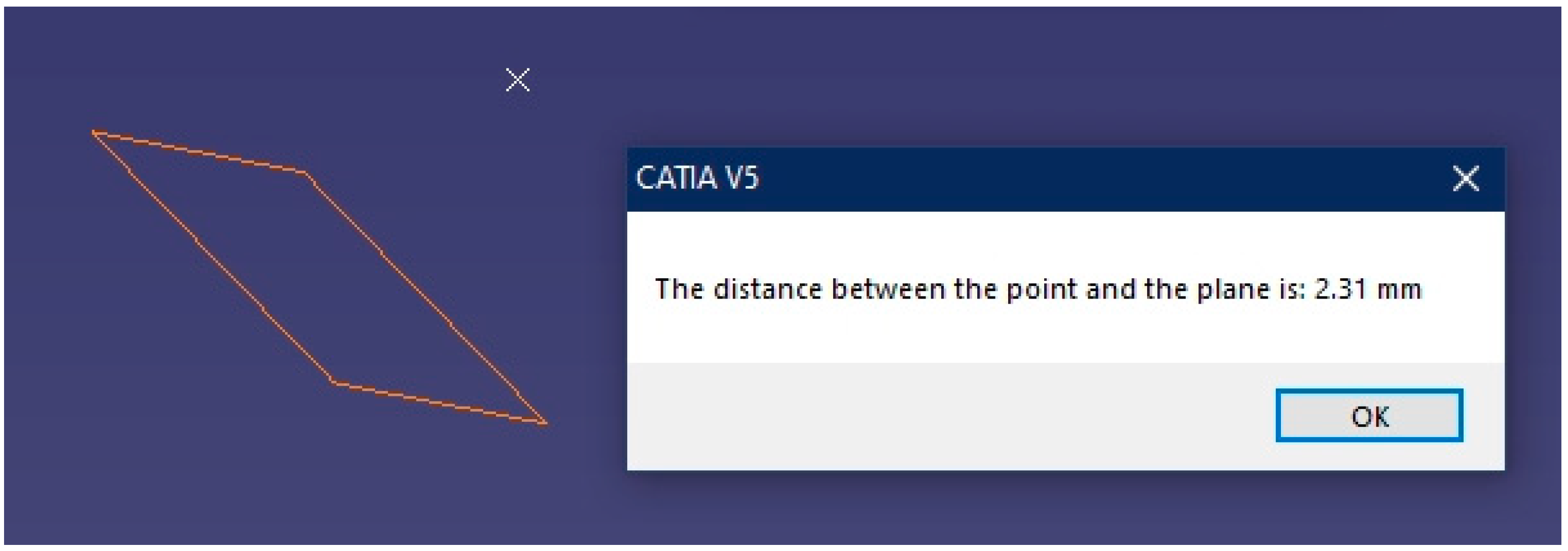
3.5.2. Distance between a Point and a Plane

In this case, any point P and any π plane are defined. For example,

$$\begin{array}{c}\mathrm{P}\left(3,1,0\right)\\ \mathsf{\pi }\equiv \mathrm{x}+\mathrm{y}+\mathrm{z}=0\end{array}$$

(21)

The geometric calculator returns the result shown in Figure 22.

As an analytical verification, the distance between the point and the plane is given by the following expression:

$$\mathrm{d}=\frac{\left|{\mathrm{Ax}}_1+{\mathrm{By}}_1+{\mathrm{Cz}}_1+\mathrm{D}\right|}{\sqrt{{\mathrm{A}}^2+{\mathrm{B}}^2+{\mathrm{C}}^2}}=\frac{\left|3.1+1.1+0.1+0\right|}{\sqrt{1^2+1^2+1^2}}=\frac{4}{\sqrt{3}}=2.31\mathrm{units}$$

(22)

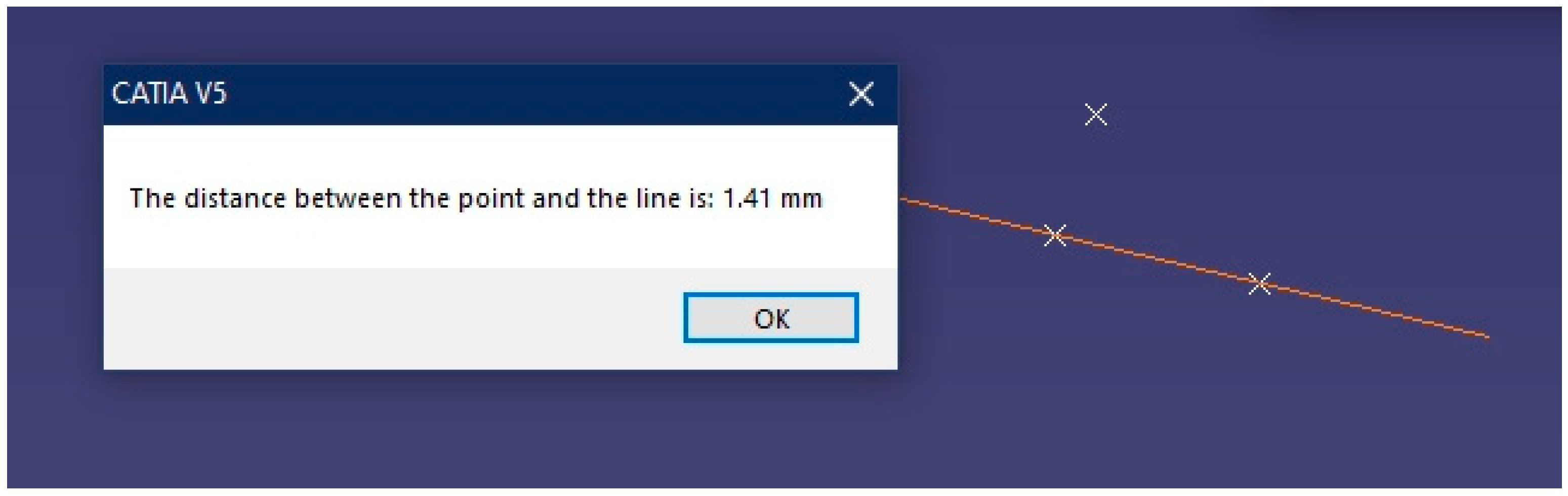
3.5.3. Distance between a Point and a Line

In this case, any point P and any line r are defined. For example,

$$\begin{array}{c}\mathrm{P}\left(3,1,0\right)\\ \mathrm{r}\equiv \{\begin{array}{c} \mathrm{x}=2+\mathsf{\lambda } \\ \mathrm{y}=-\mathsf{\lambda }\\ \mathrm{z}=2\mathsf{\lambda }\end{array}\end{array}$$

(23)

The geometric calculator returns the result shown in Figure 23.

To verify the result with the analytical solution, it is known that the distance between a point and a line is given by the application of the vector product between two vectors. First, a vector is formed between the given point P and any point Q on the line r, and the direction vector ($\overrightarrow{\mathrm{u}}$) of the line r is then multiplied.

$$\begin{array}{c}\mathrm{Q}\left(2,0,0\right)\to \overrightarrow{\mathrm{PQ}}=\left(-1,-1,0\right)\\ \overrightarrow{\mathrm{PQ}}\times \overrightarrow{\mathrm{u}}=\left|\begin{array}{ccc}\overrightarrow{\mathrm{i}}& \overrightarrow{\mathrm{j}}& \overrightarrow{\mathrm{k}}\\ -1& -1& 0\\ 1& -1& 2\end{array}\right|=\left(-2,2,2\right)\end{array}$$

(24)

Lastly, applying the expression to ascertain the distance between a point and a line, it is necessary to conduct the following calculation:

$$\mathrm{d}=\frac{|\overrightarrow{\mathrm{PQ}}\times \overrightarrow{\mathrm{u}}|}{\left|\overrightarrow{\mathrm{u}}\right|}=\frac{\sqrt{{\left(-2\right)}^2+2^2+2^2}}{\sqrt{1^2+{\left(-1\right)}^2+2^2}}=\frac{\sqrt{12}}{\sqrt{6}}=\sqrt{2}=1.41\mathrm{units}$$

(25)

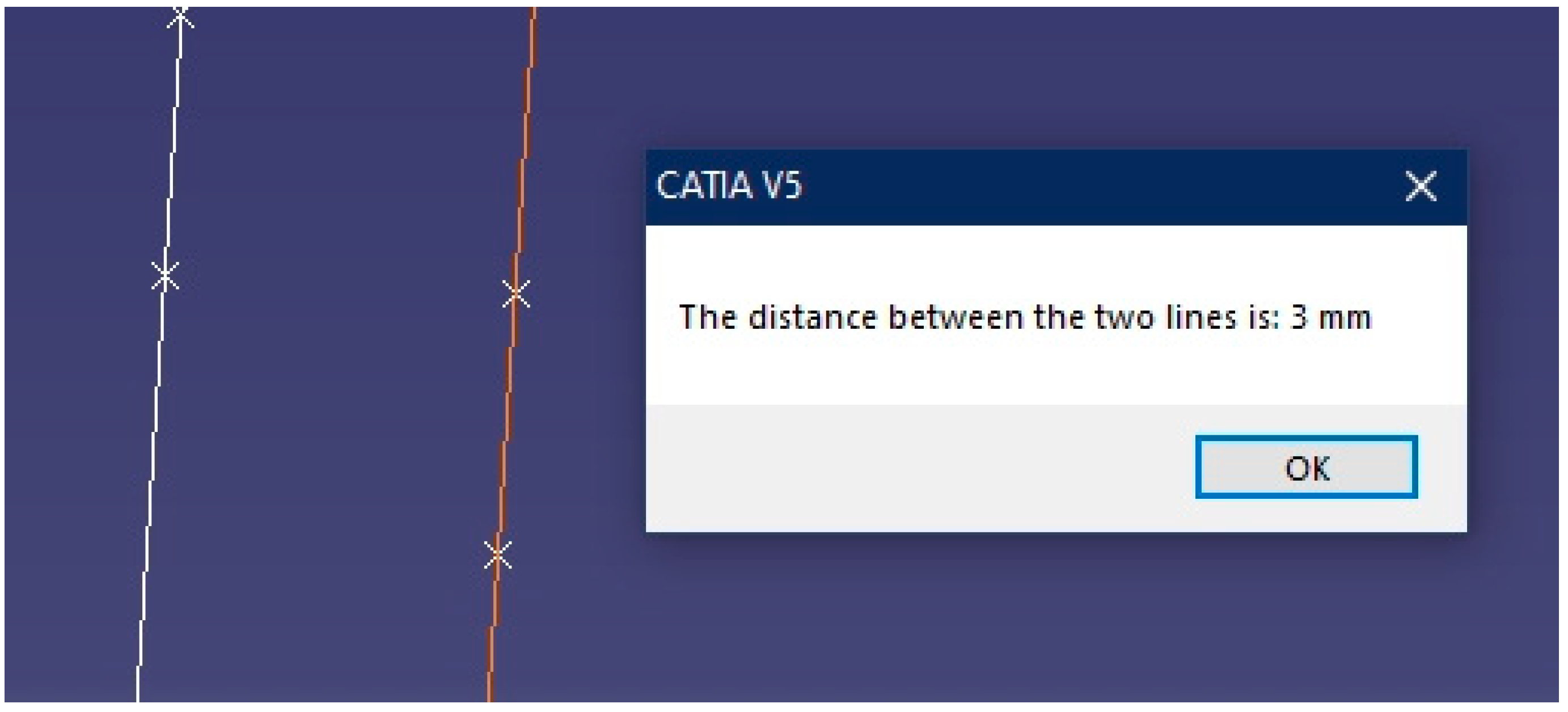
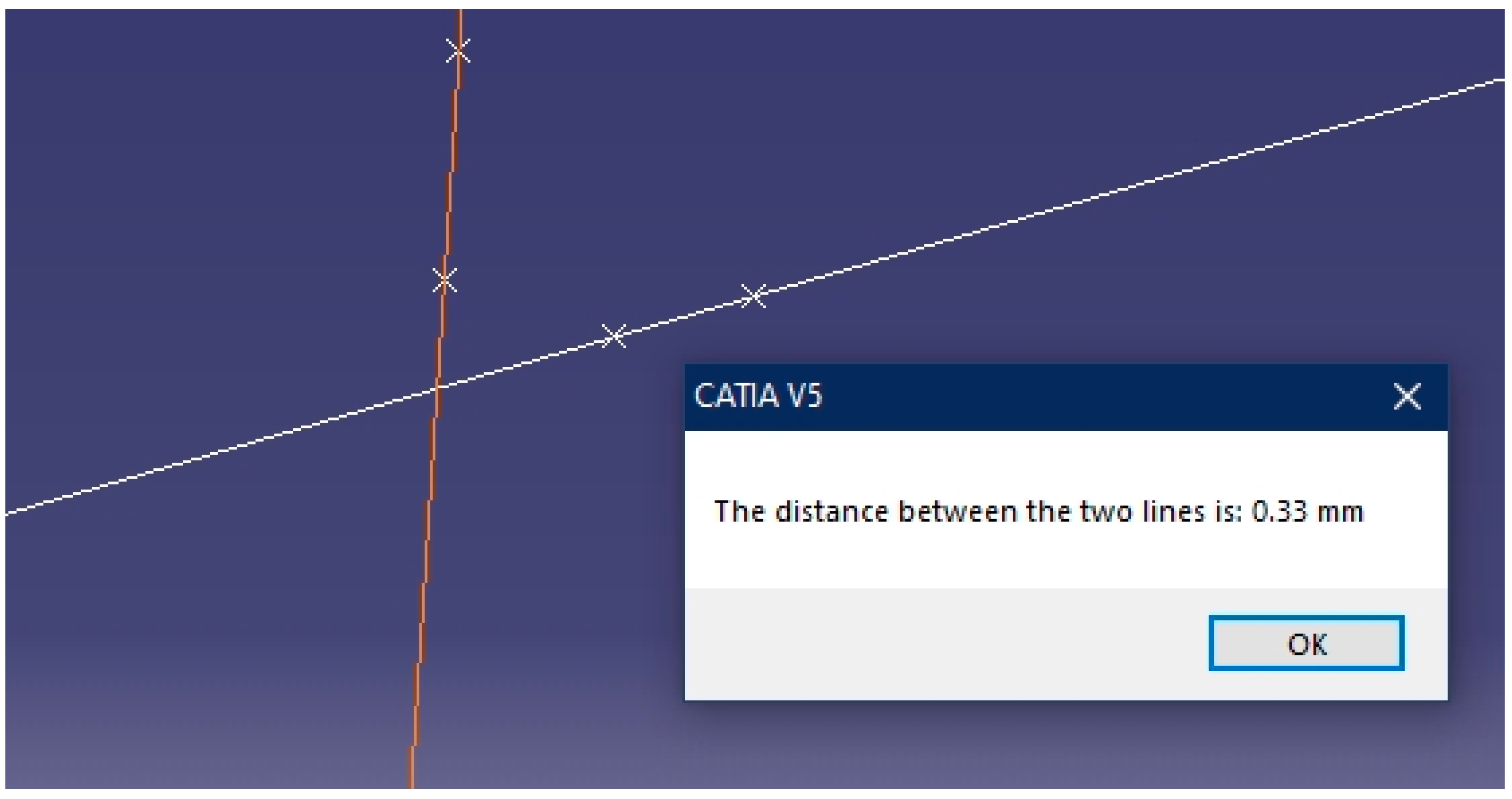
3.5.4. Distance between Two Parallel Lines

In this case, any two parallel lines r and s are defined. For example,

$$\begin{array}{c}\mathrm{r}\equiv \{\begin{array}{c} \mathrm{x}=\mathsf{\lambda } \\ \mathrm{y}=2\mathsf{\lambda }\\ \mathrm{z}=0\end{array}\\ \mathrm{s}\equiv \{\begin{array}{c} \mathrm{x}=-\mathsf{\mu }+2\\ \mathrm{y}=-2\mathsf{\mu }-1\\ \mathrm{z}=2\end{array}\end{array}$$

(26)

Once both lines are defined, the geometric calculator returns the result shown in Figure 24.

To obtain this analytically, the procedure of the previous case is followed. First, a point is obtained from each line, P and Q, and then the vector product is employed:

$$\mathrm{P}\left(0,0,0\right);\mathrm{Q}\left(2,-1,2\right)\to \overrightarrow{\mathrm{PQ}}=\left(2,-1,2\right)$$

(27)

By applying the previous Equation (25) with the direction vector ($\overrightarrow{\mathrm{u}}$) of the first line:

$$\mathrm{d}=\frac{|\overrightarrow{\mathrm{PQ}}\times \overrightarrow{\mathrm{u}}|}{\left|\overrightarrow{\mathrm{u}}\right|}=\frac{\left|\begin{array}{ccc}\overrightarrow{\mathrm{i}}& \overrightarrow{\mathrm{j}}& \overrightarrow{\mathrm{k}}\\ 2& -1& 2\\ 1& 2& 0\end{array}\right|}{\sqrt{1^2+2^2+0^2}}=\frac{\left|\left(-4,2,5\right)\right|}{\sqrt{5}}=\frac{\sqrt{{\left(-4\right)}^2+2^2+5^2}}{\sqrt{5}}=\frac{\sqrt{45}}{\sqrt{5}}=\sqrt{9}=3\mathrm{units}$$

(28)

3.5.5. Distance between Two Crossing Lines

In this case, the second line of the previous case has been modified so that it cross with the first, instead of making the lines parallel:

$$\begin{array}{c}\mathrm{r}\equiv \{\begin{array}{c} \mathrm{x}=\mathsf{\lambda } \\ \mathrm{y}=2\mathsf{\lambda }\\ \mathrm{z}=0\end{array}\\ \mathrm{s}\equiv \{\begin{array}{c} \mathrm{x}=1+\mathsf{\mu } \\ \mathrm{y}=-1\\ \mathrm{z}=1+\mathsf{\mu }\end{array}\end{array}$$

(29)

In this case, the geometric calculator returns the result shown in Figure 25.

As analytical verification, the method that is followed consists of forming a vector with two arbitrary points P and Q of the two lines, while forcing said vector to be perpendicular to the direction vectors ($\overrightarrow{\mathrm{u}} \mathrm{and}\overrightarrow{\mathrm{v}}$) of the two lines (scalar product equals to zero):

$$\begin{array}{c}\overrightarrow{\mathrm{PQ}}=\left(1+\mathsf{\mu }-\mathsf{\lambda },-1-2\mathsf{\lambda },1+\mathsf{\mu }-0\right)\\ \overrightarrow{\mathrm{PQ}}·\overrightarrow{\mathrm{u}}=1\left(1+\mathsf{\mu }-\mathsf{\lambda }\right)+2\left(-1-2\mathsf{\lambda }\right)+0\left(1+\mathsf{\mu }\right)=0\\ \overrightarrow{\mathrm{PQ}}·\overrightarrow{\mathrm{v}}=1\left(1+\mathsf{\mu }-\mathsf{\lambda }\right)+0\left(-1-2\mathsf{\lambda }\right)+1\left(1+\mathsf{\mu }\right)=0\end{array}$$

(30)

With these last two equations, the parameters are cleared and substituted to obtain the magnitude of the vector that joins the two lines:

$$\mathsf{\lambda }=-\frac{4}{9};\mathsf{\mu }=-\frac{11}{9}\to \mathrm{d}=|\overrightarrow{\mathrm{PQ}}|=\sqrt{\frac{9}{81}}=\frac{1}{3}=0.33\mathrm{units}$$

(31)

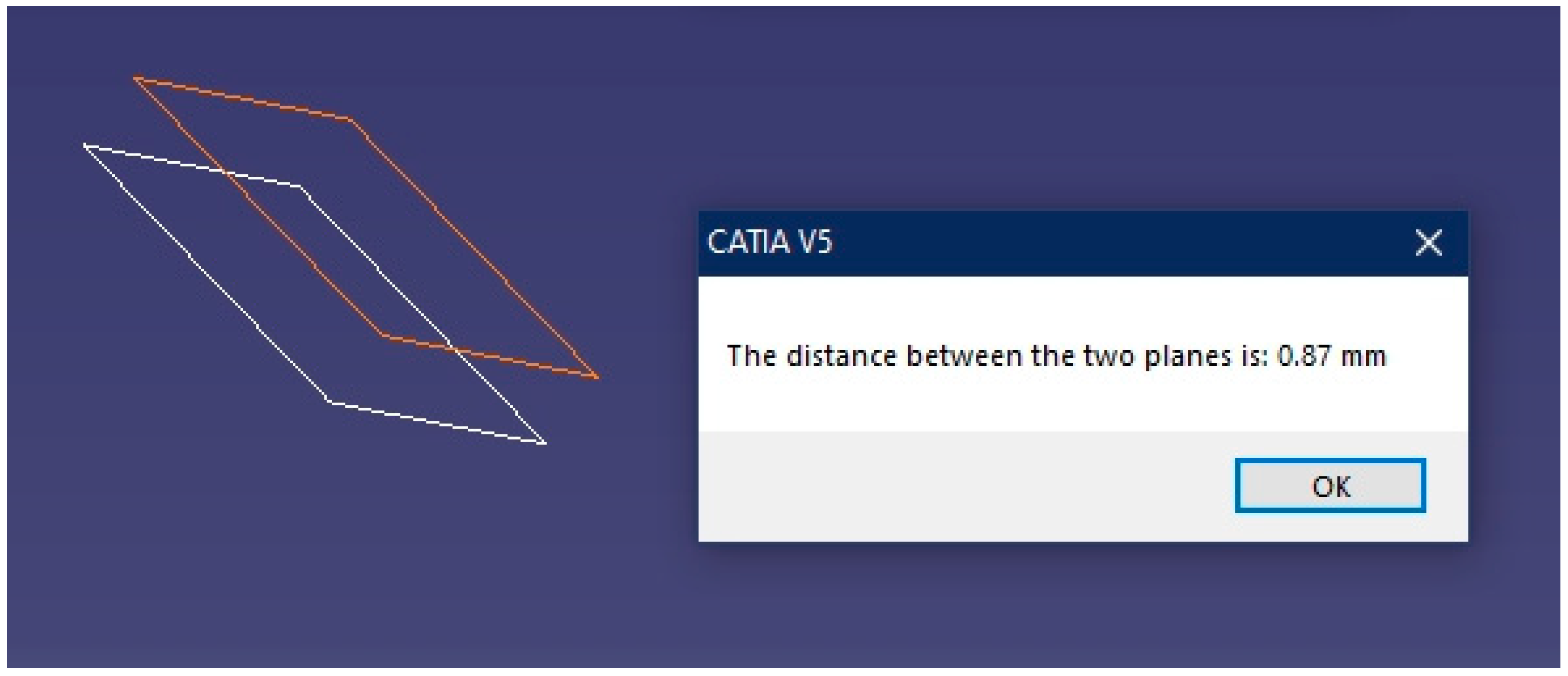
3.5.6. Distance between Two Planes

Obviously both planes must be parallel. Let any two planes be ${\mathsf{\pi }}_1{\mathrm{and}\mathsf{\pi }}_2$.

$$\begin{array}{c}{\mathsf{\pi }}_1\equiv \mathrm{x}+\mathrm{y}+\mathrm{z}=0\\ {\mathsf{\pi }}_2\equiv 2\mathrm{x}+2\mathrm{y}+2\mathrm{z}-3=0\end{array}$$

(32)

Once both planes are defined, the geometry calculator returns the result shown in Figure 26.

To calculate the distance between the two planes analytically, any point P on the first plane ${\mathsf{\pi }}_1$ is considered, and the corresponding formula is applied:

$$\begin{array}{c}\mathrm{P}\left(1,-2,1\right)\\ \mathrm{d}=\frac{\left|{\mathrm{A}}_2{\mathrm{x}}_1+{\mathrm{B}}_2{\mathrm{y}}_1+{\mathrm{C}}_2{\mathrm{z}}_1+{\mathrm{D}}_2\right|}{\sqrt{{\mathrm{A}}_2^2+{\mathrm{B}}_2^2+{\mathrm{C}}_2^2}}=\frac{\left|2.1+2·\left(-2\right)+2.1-3\right|}{\sqrt{2^2+2^2+2^2}}=\frac{\sqrt{3}}{2}=0.87\mathrm{units}\end{array}$$

(33)

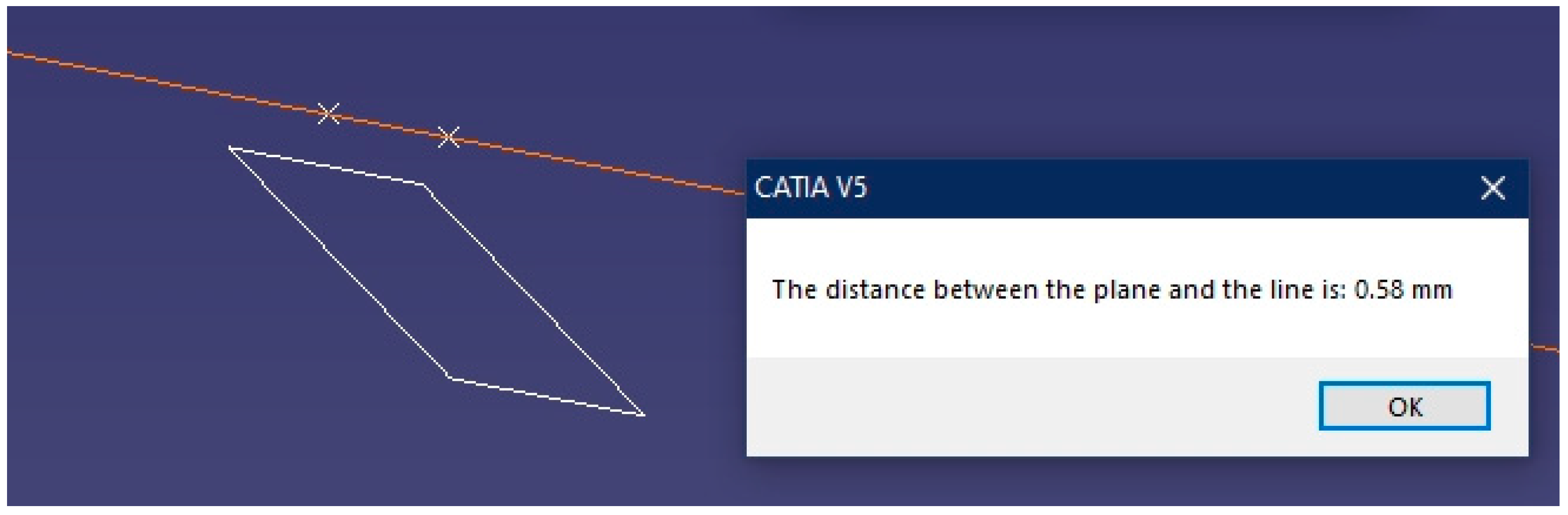
3.5.7. Distance between a Line and a Plane

Obviously, the two elements must be parallel to each other. To this end, by reusing the geometric elements that are parallel to each other, previously created in Section 3.2, the distance between the line and the plane can be measured:

$$\begin{array}{c}\mathrm{r}\equiv \{\begin{array}{c}\mathrm{x}=4\mathsf{\lambda } \\ \mathrm{y}=2-\mathsf{\lambda }\\ \mathrm{z}=-1-3\mathsf{\lambda }\end{array}\\ \mathsf{\pi }\equiv \mathrm{x}+\mathrm{y}+\mathrm{z}=0\end{array}$$

(34)

In this case, the application shows the result presented in Figure 27.

As analytical verification, it is known that the distance between the plane and the line is the same as that between the plane and any point thereon. Therefore, the point with which the line was defined (Section 3.2.) can be employed:

$$\begin{array}{c}\mathrm{P}\left(0,2,-1\right)\\ \mathsf{\pi }\equiv \mathrm{x}+\mathrm{y}+\mathrm{z}=0\end{array}$$

(35)

By applying the expression that determines the distance between the point and the plane,

$$\mathrm{d}=\frac{\left|{\mathrm{Ax}}_1+{\mathrm{By}}_1+{\mathrm{Cz}}_1+\mathrm{D}\right|}{\sqrt{{\mathrm{A}}^2+{\mathrm{B}}^2+{\mathrm{C}}^2}}=\frac{\left|0.1+2.1+\left(-1\right)·1+0\right|}{\sqrt{1^2+1^2+1^2}}=\frac{\sqrt{3}}{3}=0.58\mathrm{units}$$

(36)

3.6. Analysis of Errors

It is interesting to consider what happens in the event when a value not accepted by the application is entered. In this scenario, a non-numeric value could be entered in some form; alternatively, when generating the line, the direction vector could be null, or the three points given to create a plane could be aligned, among other cases.

For all these examples, CATIA would show an error message of the geometric type itself, not due to the programming of the macro; hence, the addition of redundant error messages has not been considered.

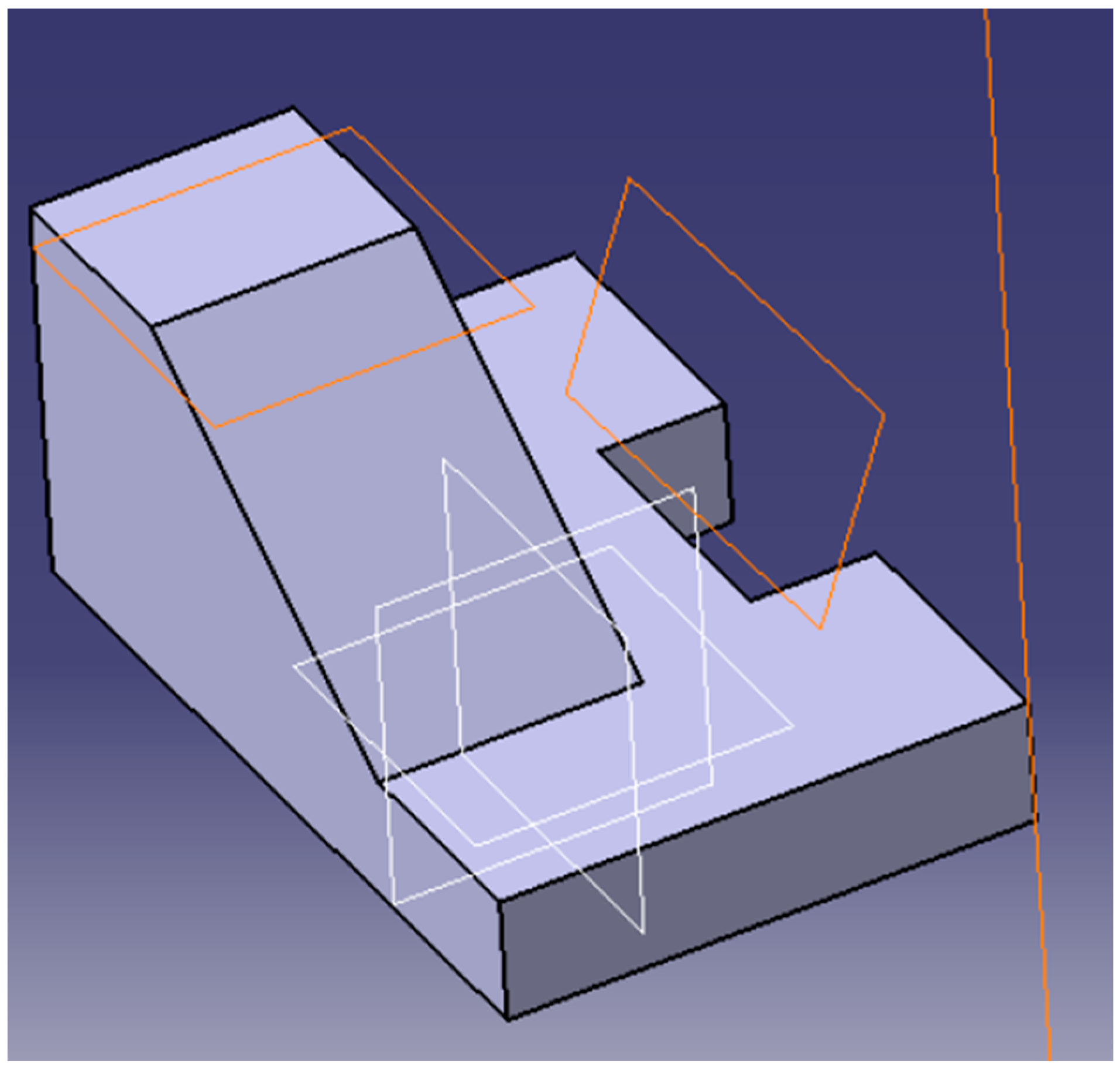
3.7. Integration with Three-Dimensional Solids

Lastly, the source code of the geometric calculator was modified so that it could also work with three-dimensional models designed in CATIA with the “Part Design” module. These models present the particularity of working with vertices, edges, and faces, instead of with points, lines, and planes, which were the elements utilized by the surfaces. To this end, the possibility of selecting these entities has been included in the source code of the geometric calculator.

In this way, the geometric calculator enables the measurement of the angles that exist between the faces of the part, the distance between faces, and the distance between vertices, among other elements.

In Figure 28, an example can be appreciated of how the geometric calculator creates new entities in the environment of a three-dimensional solid, to continue modeling new parts of the piece, for dimensioning reasons, or for another reason.

4. Conclusions and Future Developments

This article presented the design and development of an application consisting of a geometric calculator developed as a macro in CATIA V5R21. Said macro consists of two independent modules: one that contemplates the creation of the three geometric elements (point, line, and plane), and another module that solves five types of general geometric problems (points of intersection, definition of lines, and definition of planes, angles, and distances).

The scientific contribution of the research lies in the fact that it is the only geometric application currently in existence that is integrated into a 3D CAD environment such as CATIA V5, unlike existing software such as GEUP 3D and Geogebra which work in geometric environments other than CAD 3D. Its novelty makes this application a very powerful tool in the 3D design process in the CATIA V5 environment.

The macro is developed with the Visual Basic for Applications (VBA) language, and it is highly useful, not only from the educational point of view as a support in the teaching of subjects related to engineering graphics (including graphic expression, descriptive geometry, and technical drawing), but also from a professional point of view, since it allows its integration with real three-dimensional models, which helps in the metric consultation of angles and distances. Likewise, it was verified how all the results obtained with the macro coincide with the results obtained through analytical geometry, which led to the validation of the developed application.

The work module utilized in the CATIA V5R21 environment is “Wireframe and Surface Design” since it makes it possible to work with the three geometric elements (point, line, and plane), and the aforementioned macro was programmed within said module. The macro makes it possible to enter data easily through forms with an illustrative graphic appearance and intuitive images.

As for future developments, the following can be established:

• The incorporation of new geometric problems that involve curved surfaces, surfaces of revolution, and three-dimensional solids.
• The integration of new operational modules such as intersections between solids or surfaces and their two-dimensional development.
• The representation of the results obtained as dihedral projections utilizing the CATIA V5 “Drafting” module, which would enable problems to be solved in a simple and semi-automatic way.

References

1. Anton, D.; Amaro-Mellado, J.L. Engineering graphics for thermal assessment: 3D thermal data visualization based on infrared thermography, GIS and 3D point cloud processing software. Symmetry 2021, 13, 335. [Google Scholar] [CrossRef]
2. Zhang, Y.H.; Su, B.B. The design and implementation of roadworks management system based on GIS. In Proceedings of the 2nd International Conference on Civil, Architectural and Hydraulic Engineering (ICCAHE 2013), Zhuhai, China, 27–28 July 2013. [Google Scholar]
3. Rojas-Sola, J.I.; De la Morena-de la Fuente, E. The Hay inclined plane in Coalbrookdale (Shropshire, England): Geometric modeling and virtual reconstruction. Symmetry 2019, 11, 589. [Google Scholar] [CrossRef] [Green Version]
4. Rojas-Sola, J.I.; Hernandez-Diaz, D.; Villar-Ribera, R.; Hernandez-Abad, V.; Hernandez-Abad, F. Computer-Aided Sketching: Incorporating the locus to improve the three-dimensional geometric design. Symmetry 2020, 12, 1181. [Google Scholar] [CrossRef]
5. Wellman, B.L. Technical Descriptive Geometry, 2nd ed.; WCB McGraw-Hill: New York, NY, USA, 1987. [Google Scholar]
6. Postnikov, M. Analytic Geometry; URSS: Moscow, Russia, 1994. [Google Scholar]
7. Giesecke, F.E. Technical Drawing with Engineering Graphics, 14th ed.; Pearson: Harlow, UK, 2014. [Google Scholar]
8. Spivak, S.M.; Brenner, F.C. Standardization Essentials: Principles and Practice, 1st ed.; CRC Press: Boca Ratón, FL, USA, 2001. [Google Scholar]
9. De Risi, V. (Ed.) Mathematizing Space: The Objects of Geometry from Antiquity to the Early Modern Age; Birkhäuser: Basel, Switzerland, 2015. [Google Scholar]
10. Friberg, J. Methods and Traditions of Babylonian Mathematics. Hist. Math. 1981, 8, 277–318. [Google Scholar] [CrossRef] [Green Version]
11. Merzbach, U.C.; Boyer, C.B. A History of Mathematics, 3rd ed.; John Wiley & Sons: Hoboken, NJ, USA, 2011. [Google Scholar]
12. GEUP3D8. Available online: https://www.geup.net/es/geup3d/index.htm (accessed on 2 February 2023).
13. GeoGebra. Available online: https://www.geogebra.org (accessed on 2 February 2023).
14. Essen, H.; Svensson, M. Calculation of coordinates from molecular geometric parameters and the concept of a geometric calculator. Comput. Chem. 1996, 20, 389–395. [Google Scholar] [CrossRef]
15. Tickoo, S. CATIA V5R21 for Designers; CADCIM Technologies: Schererville, IN, USA, 2014. [Google Scholar]
16. Rojas-Sola, J.I.; Del Río-Cidoncha, G.; Ortíz-Marín, R.; López-Pedregal, J.M. Design and development of sheet-metal elbows using programming with visual basic for applications in CATIA. Symmetry 2020, 13, 33. [Google Scholar] [CrossRef]
17. Rojas-Sola, J.I.; Del Río-Cidoncha, G.; Ortíz-Marín, R.; Moya-Ocaña, J.A. Design and development of a macro for comparing sections of planes to parts using programming with visual basic for applications in CATIA. Symmetry 2023, 15, 242. [Google Scholar] [CrossRef]
18. Ross, E. VB Scripting for CATIA v5: How to Program CATIA Macros; Createspace Independent Pub: Scott Valley, CA, USA, 2012. [Google Scholar]
Figure 1. Shortcut icon (red circle) from the “Wireframe and Surface Design” module toolbar.
Symmetry 15 00547 g001
Figure 2. Flowchart of the operation of the developed macro.
Symmetry 15 00547 g002
Figure 3. Main form of Module 1: generation of geometric elements.
Symmetry 15 00547 g003
Figure 4. Form for creating a point (left) and graphic result (right).
Symmetry 15 00547 g004
Figure 5. Forms for creating a line: main form (left) and intermediate form (right).
Symmetry 15 00547 g005
Figure 6. Forms for creating a plane: main form (left) and intermediate form (right).
Symmetry 15 00547 g006
Figure 7. Main form of Module 2: geometric calculator.
Symmetry 15 00547 g007
Figure 8. Form to find points of intersection.
Symmetry 15 00547 g008
Figure 9. Form to find lines.
Symmetry 15 00547 g009
Figure 10. Form to find planes.
Symmetry 15 00547 g010
Figure 11. Form to calculate angles.
Symmetry 15 00547 g011
Figure 12. Form to calculate distances.
Symmetry 15 00547 g012
Figure 13. Point of intersection between two lines.
Symmetry 15 00547 g013
Figure 14. Point of intersection between a line and a plane.
Symmetry 15 00547 g014
Figure 15. Point of intersection between three planes.
Symmetry 15 00547 g015
Figure 16. Line that passes through a point and is parallel to two planes together with its parametric equation.
Symmetry 15 00547 g016
Figure 17. Plane that passes through a point and is perpendicular to a line, together with its parametric equation.
Symmetry 15 00547 g017
Figure 18. Angle between two lines.
Symmetry 15 00547 g018
Figure 19. Angle between a line and a plane.
Symmetry 15 00547 g019
Figure 20. Angle between two planes.
Symmetry 15 00547 g020
Figure 21. Distance between two points.
Symmetry 15 00547 g021
Figure 22. Distance between a point and a plane.
Symmetry 15 00547 g022
Figure 23. Distance between a point and a line.
Symmetry 15 00547 g023
Figure 24. Distance between two parallel lines.
Symmetry 15 00547 g024
Figure 25. Distance between two crossing lines.
Symmetry 15 00547 g025
Figure 26. Distance between two planes.
Symmetry 15 00547 g026
Figure 27. Distance between a line and a plane.
Symmetry 15 00547 g027
Figure 28. New lines and planes generated (in orange) from a three-dimensional solid modeled in CATIA.
Symmetry 15 00547 g028