Increasing the Accuracy of Soil Nutrient Prediction by Improving Genetic Algorithm Backpropagation Neural Networks

Abstract

Soil nutrient prediction has been eliciting increasing attention in agricultural production. Backpropagation (BP) neural networks have demonstrated remarkable ability in many prediction scenarios. However, directly utilizing BP neural networks in soil nutrient prediction may not yield promising results due to the random assignment of initial weights and thresholds and the tendency to fall into local extreme points. In this study, a BP neural network model optimized by an improved genetic algorithm (IGA) was proposed to predict soil nutrient time series with high accuracy. First, the crossover and mutation operations of the genetic algorithm (GA) were improved. Next, the IGA was used to optimize the BP model. The symmetric nature of the model lies in its feedforward and feedback connections, i.e., the same weights must be used for the forward and backward passes. An empirical evaluation was performed using annual soil nutrient data from China. Soil pH, total nitrogen, organic matter, fast-acting potassium, and effective phosphorus were selected as evaluation indicators. The prediction results of the IGA–BP, GA–BP, and BP neural network models were compared and analyzed. For the IGA–BP prediction model, the coefficient of determination for soil pH was 0.8, while those for total nitrogen, organic matter, fast-acting potassium, and effective phosphorus were all greater than 0.98, exhibiting a strong generalization ability. The root-mean-square errors of the IGA–BP prediction models were reduced to 50% of the BP models. The results indicated that the IGA–BP method can accurately predict soil nutrient content for future time series.

1. Introduction

A soil nutrient is one of the essential nutrients that plants absorb from the soil; it facilitates crop growth and nutrient absorption. Soil fertility directly affects the growth and yield of crops, and it is related to the sustainable development of agriculture in China [1]. Therefore, the accurate prediction of soil nutrient content not only directly affects food production and precise fertilization in China but is also significant for precision agriculture and agricultural production efficiency [2]. The entire growth and development processes of crops can be divided into several sub-growth cycles, each of which requires different nutrients. To study the demands of soil nutrients in crop growth and development, researchers have introduced the concept of soil nutrient time series to describe temporal variations in soil nutrients. A soil nutrient time series predicts the evolution of soil nutrients in a region over a certain period. It is based on the massive soil data of the region. In accordance with the specific crops grown in a region and the established soil nutrient time evolution model, actual soil nutrient requirements for specific crops are calculated and used as a guide for the precise fertilization of the crop growing process. Traditional soil nutrient testing methods mostly use field sampling and laboratory chemical analysis, which are time-consuming and labor-intensive, require numerous chemicals, and cause environmental pollution [3]. With the rapid developments in the field of machine learning, the use of machine learning technologies in predicting nutrients in soil and crops has become a major subject of interest [4,5,6,7].

The backpropagation (BP) neural network is one of the most widely used neural networks. It is a feedforward learning algorithm and an error BP neural network that is widely used in the field of intelligent computing [8,9,10,11]. This method iteratively adjusts the weights and thresholds of a network in accordance with the negative gradient descent direction, minimizing the training error of the objective function. The algorithm results are gradually corrected through the reverse transfer of error. Moreover, a BP neural network exhibits strong self-learning and nonlinear mapping abilities [12,13]. A BP neural network was used to predict soil erosion and nutrient content in runoff near Lincoln, Nebraska, USA. The results showed that the neural network model can estimate nutrients in runoff [14]. Cross et al. [15] developed an artificial neural network for the online identification of cohesion and the internal friction angle. The neural network model was used to predict dynamic changes in soil moisture content for irrigation scheduling. It had a learning rate of 0.1, a maximum number training time of 500, and a minimum mean square error of 0.001 [16]. Li et al. [17] established an error BP neural network prediction model with different time spans to predict soil moisture content in Feidong County, Anhui Province, China. The results exhibited good prediction accuracy. BP neural networks were applied for comprehensive soil nutrient evaluation [18]. The random selection of the initial threshold and weight of a single BP neural network model has led to some problems, such as poor robustness of the prediction model and large errors in the prediction results, when determining soil nutrient grading. Therefore, traditional BP neural networks have some limitations, such as low convergence speed, sensitivity to weight initialization, and easily falling into local extremes [19,20].

Genetic algorithms (GAs) are stochastic search methods that mimic the process through which natural biological evolution works by applying the principle of survival of the fittest. GAs operate on a set of potential solutions to produce good solutions and accurate prediction values [21]. They are effective in optimizing the structure, weight, and threshold of BP neural networks and in addressing disadvantages, such as slow convergence speed, difficult structure determination, and tendency to fall into the local optimum, when neural networks are used [22]. To prevent the sawtooth phenomenon in neural networks optimized by GAs, an adaptive genetic neural network algorithm was proposed to improve the prediction accuracy and efficiency of soil moisture [23]. A genetic radial basis neural network was constructed to analyze effective zinc in soil. The results were compared with those of traditional neural networks, and the genetic radial basis neural network achieved higher prediction accuracy [24]. The symmetric nature of the model lies in its feedforward and feedback connections, i.e., the same weights must be used for forward and backward passes. The GA–BP neural network was used to predict the soil shear parameters of lunar weathering layers. The experimental results showed that the GA–BP algorithm demonstrated better performance in identifying soil shear parameters than the BP algorithm [25].

To increase the convergence speed of a traditional BP neural network model, an improved GA (IGA) was used to optimize the neural network model. The week-by-week water quality of pH value from Bengbu Gate in Bengbu City, Anhui Province, China, was selected as the research object, and the water quality prediction results showed that the model presented strong generalization ability [26]. The IGA–BP neural network was used to calibrate binocular cameras [27]. The experimental results showed that the method yielded better results in the process of the binocular cameras and could meet the requirements of binocular camera calibration. The IGA–BP neural network was applied to establish the relationship between maize yield and an underground drip irrigation system [28]. The average error of the model was only 0.71%. This method accelerated the convergence speed of the network and improved prediction accuracy, enabling it to describe the relationship between irrigation water and maize yield more accurately.

GA exhibits the advantages of globality, parallelism, good adaptability, and robustness. It is an ideal algorithm for optimizing BP neural networks. It can effectively address many problems, such as the tendency of BP neural networks to fall into the local minimum and slow convergence speed. In this study, a GA was further improved in accordance with the number of input and output neurons, the number of neurons in the hidden layers, the coding method, the fitness function, and the genetic operation on the results of BP neural networks. An IGA was proposed to optimize the BP neural network (IGA–BP) and used in establishing a time series soil nutrient prediction model. The second section of this paper focuses on the data sources, the IGA–BP model implementation method, and the prediction process. The third section discusses the prediction results of the three modeling approaches for five soil nutrient components. The fourth section summarizes the entire text.

2. Materials and Methods

2.1. Study Site and Data Sources

Ningguo City is located in southeastern Anhui Province, on the northeast side of the mountainous area of southern Anhui. The ground spans between 30016′–30047′ north latitude and 118036′–119024′ east longitude, with an altitude of 1587 m. It has a sub-tropical monsoon climate, mild climate, abundant rainfall, sufficient sunshine, and four distinct seasons. The average annual precipitation is 1426 mm. Its soil types are red soil with flat stones and yellow-red soil with flat stones. In this study, the monthly content data of soil organic matter, total nitrogen, available phosphorus, available potassium, available iron, available manganese, available copper, available zinc, pH value, and other components were collected from the Chinese soil nutrient analysis database. Soil nutrient analysis data from the years 2008–2015 for 18 townships in Ningguo City were obtained. On the basis of differences in soil types and crops grown, soil data from six townships were selected as the research objects in this study. The monthly soil composition data from the years 2008–2013 were used as the training set. Meanwhile, the soil composition data from the years 2014–2015 were used as the validation set. The distribution of soil nutrient sampling points (triangular points) is illustrated in Figure 1. The latitude and longitude of the sampling points are provided in

Table 1. Latitude and longitude of sampling points.

Township Name	Zhufeng Street	Gangkou Town	Jialu Town	Wangxi Street	Xiaxi Town	Zhongxi Town
Latitude (°)	30.5651	30.6902	30.4329	30.6902	30.5064	30.4942
Longitude (°)	118.9462	118.9896	118.8619	118.9896	118.9501	119.1702

. As shown in Figure 1, the six points are scattered and representative. These points represent the prediction results of different towns.

2.2. IGA–BP Neural Network Prediction Model of Soil Nutrient

In soil nutrient prediction, the traditional GA improves the optimization ability of the initial threshold and weight of a BP neural network. However, this method separates the hidden layer neural nodes from their corresponding weights and thresholds. Thus, it increases the risk of falling into local extreme values. Ultimately, this method produces an inaccurate soil nutrient time series. In this study, the IGA–BP method started from the shortcomings of GA in soil nutrient time series prediction and improved the convergence and global optimization abilities of GA. The hidden layer neural nodes of the BP neural network were connected with their corresponding weights and thresholds, and thus the BP neural network could obtain the optimal weights and thresholds, improving its performance.

2.2.1. Determination of Number of Neurons

In accordance with Kolmogorov’s theorem, a three-layer BP neural network can approximate any nonlinear function with arbitrary precision under the conditions of a reasonable structure and appropriate weights. On the basis of this theorem, the BP neural network model selected the network structure with input, hidden, and output layers. This three-layer network structure had single-layer network nodes.

The number of nodes in the hidden layer of the BP neural network was determined by the number of nodes in the input and output layers:

$$hl=\sqrt{\left(il+ol\right)}+a,$$

(1)

where hl is the number of hidden layer nodes, il is the number of input layer nodes, ol is the number of output layer nodes, and a is an arbitrary constant between 0 and 10.

2.2.2. Encoding Scheme

In this study, we used mixed real number encoding to optimize the weights and thresholds of the BP neural network. The real number was directly used as a gene locus of a chromosome, considerably shortening the length of the chromosome. This process not only eliminated the tediousness of encoding and decoding back and forth, but it also reduced computational volume, improved computational accuracy, and enhanced the search ability of the solution space.

Each individual was a string of real numbers during the initialization of the initial weights and thresholds of the GA optimization neural network that consisted of the threshold value b_i for the neuron in the output layer, the threshold value B_i for the neuron in the hidden layer, and the connection weight W_i of the neuron in the output layer with the input layer. Each weight and threshold were encoded with a real number. The coding of all the weights and thresholds were connected to form an individual coding. The parameters to be optimized in the BP network were filled into the corresponding positions of the individual code, as shown in Figure 2. The corresponding weights and thresholds were selected in accordance with the corresponding positions when decoding. Among them, the thresholds and connection weights of the hidden layer neurons were $\left(1+s_i+s_o\right)\ast s_h$. Therefore, the effective length of the individuals in the IGA scheme was

$$L=s_o+\left(1+s_i+s_o\right)\ast s_h,$$

(2)

where s_i, s_o, and s_h denote the number of neurons in the input, output, and hidden layers, respectively.

This real number encoding method associated the implicit layer nodes with the connection weights to improve the convergence speed of the algorithm to a certain extent. In addition, it effectively reduced computational effort and quantization error when compared with traditional binary encoding.

2.2.3. Adaptation Function

The selection operator used in traditional GA exhibits a large error in the actual selection process. To address this problem, the fitness ranking method was used in this study. For each individual in the population, the sum of the differences between its true and predicted values at all moments, denoted as E, was calculated as follows:

$$E=\frac{1}{2}{{\displaystyle \sum }}_{k=1}^m{{\displaystyle \sum }}_{i=1}^{ol}\left(y_i^k-o_i^k\right),$$

(3)

where E denotes each sample that corresponds to each individual in the current population and is also the difference between the true and predicted values for all moments, m denotes the training sample volume of the soil nutrient to be predicted, ol denotes the number of output nodes, and $y_i^k-o_i^k$ denotes the error between the actual value of the k-th sample relative to the i-th output value.

The fitness function was

$$F=\frac{1}{E}.$$

(4)

The greater the fitness, the greater the probability of being selected. The computation process sorted fitness to produce new populations by ranking them from largest to smallest.

The relative fitness function was defined as

$$F_l^{\prime }=\frac{F_l-F_{min}}{F_{max}-F_{min}}.$$

(5)

F_max and F_min indicate the maximum and minimum fitness values in the current population, respectively.

2.2.4. Crossover and Variation Operators

Crossover probability determines the diversity of the data population and the global merit-seeking ability of the GA. Variance probability determines whether the GA can avoid local extremes. Therefore, the two core factors of GAs are crossover probability and variation probability.

Linear crossover and convex crossover are the commonly used arithmetic crossover methods. Linear crossover exhibits the possibility of exceeding the range of values, while convex crossover produces offspring located between two parents and remains valid. To achieve excellent crossover results, i.e., fast and guaranteed to meet the constraints, this study combined linear crossover and convex crossover to construct a new multipoint crossover operator.

We denoted the crossover probability as $p_c.$ A cross-selected individual Xrs with the same effective length as the parent chromosome was constructed. Gene position was 0 or 1. When $x_{rsc}$ was $0$, the parent chromosome did not cross over. When $x_{rsc}$ was 1, the parent chromosomes $Xr$ and $Xs$ crossed over, and the selected crossover position was c. The corresponding crossover genes were $x_{rc}$ and $x_{sc}$. The corresponding genes after the crossover were $x_{rc}{}^{\prime }$ and $x_{sc}{}^{\prime }$.

If individual $X_r$ was better than individual $X_s$, i.e., $F_r^{\prime }>F_s^{\prime }$, then

$${\mathrm{X}}_{\mathrm{rc}}{}^{\prime }=\left\{\begin{array}{c}{\mathrm{x}}_{\mathrm{rc}}+\mathrm{b}\ast {\mathrm{rand}}_1\ast \left({\mathrm{M}}_{\mathrm{c}}-{\mathrm{x}}_{\mathrm{sc}}\right),{\mathrm{x}}_{\mathrm{rc}}>{\mathrm{x}}_{\mathrm{sc}}\\ {\mathrm{x}}_{\mathrm{sc}}+\mathrm{b}\ast {\mathrm{rand}}_1\ast \left({\mathrm{N}}_{\mathrm{c}}-{\mathrm{x}}_{\mathrm{rc}}\right),{\mathrm{x}}_{\mathrm{rc}}\le {\mathrm{x}}_{\mathrm{sc}}\end{array}\right.,$$

(6)

$${\mathrm{X}}_{\mathrm{sc}}{}^{\prime }={\mathrm{x}}_{\mathrm{sc}}+\mathrm{d}\ast \left({\mathrm{x}}_{\mathrm{rc}}-{\mathrm{x}}_{\mathrm{sc}}\right),$$

(7)

$$b=\left\{\begin{array}{c}1-\frac{t}{T},x_{rc}=x_{sc}\\ 1,other\end{array}\right..$$

(8)

If individual $X_r$ was not better than individual $X_s$, i.e., $F_r^{\prime }<F_s^{\prime }$, then

$${\mathrm{X}}_{\mathrm{sc}}{}^{\prime }=\left\{\begin{array}{c}{\mathrm{x}}_{\mathrm{sc}}+\mathrm{b}\ast {\mathrm{rand}}_1\ast \left({\mathrm{N}}_{\mathrm{c}}-{\mathrm{x}}_{\mathrm{sc}}\right),{\mathrm{x}}_{\mathrm{rc}}>{\mathrm{x}}_{\mathrm{sc}}\\ {\mathrm{x}}_{\mathrm{rc}}+\mathrm{b}\ast {\mathrm{rand}}_1\ast \left({\mathrm{M}}_{\mathrm{c}}-{\mathrm{x}}_{\mathrm{sc}}\right),{\mathrm{x}}_{\mathrm{rc}}\le {\mathrm{x}}_{\mathrm{sc}}\end{array}\right.,$$

(9)

$${\mathrm{X}}_{\mathrm{rc}}{}^{\prime }=\left\{\begin{array}{c}{\mathrm{x}}_{\mathrm{rc}}+\mathrm{b}\ast {\mathrm{rand}}_1\ast \left({\mathrm{N}}_{\mathrm{c}}-{\mathrm{x}}_{\mathrm{rc}}\right),{\mathrm{x}}_{\mathrm{rc}}={\mathrm{x}}_{\mathrm{sc}}\\ {\mathrm{x}}_{\mathrm{rc}}+\mathrm{d}\ast \left({\mathrm{x}}_{\mathrm{sc}}-{\mathrm{x}}_{\mathrm{rc}}\right),\mathrm{other}\end{array}\right.,$$

(10)

where 0 < d < 1; rand₁ represents a random number between (0, 1); t represents the evolutionary algebra; T represents the maximum evolutionary algebra; and Mc and Nc represent the upper and lower limits of the value of the gene xc in the constraints, respectively. When the above crossover operations were completed, the corresponding offspring chromosomes could be obtained.

We denoted the mutation probability as $p_m$. $x_{je}$ represents the e-th gene in the j-th individual in the parent; $L$ is the effective length; $x_{je}{}^{\prime }$ represents the e-th gene in the j-th individual in the offspring; and $1\le j\le popNum,1\le e\le L$.

$$x_{je}{}^{\prime }=\left\{\begin{array}{c}{N}_e+ran{d}_2\ast \left(M_e-N_j\right),ran{d}_2<p_m\\ x_{je},\mathrm{other}\end{array}\right.,$$

(11)

where rand₂ represents a random number between 0 and 1. When rand₂ < p_m represents actual mutation, Me and Ne represents the upper and lower limits, respectively, of the value range of the gene x_e of any individual in the constraints.

With these crossover and variation operators, the individuals in the population mutate with a controlled range of variation in accordance with probability. The variation of individual may mutate, increasing the diversity of individuals in the offspring. Optimal individuals were selected from the current population, and their corresponding weights and thresholds were regarded as the optimal weights and thresholds. The optimal weights and thresholds were used to train the BP neural network, solve the problem of falling into the local minimum during training, and obtain the IGA–BP neural network model. The entire algorithm flow of the improved GA (Algorithm 1) optimized the BP neural network for soil nutrient prediction, as shown in Figure 3.

Algorithm 1 The improved GA

Input: $T_s$: Training set $V_s$: Validation set $G$: Maximum number of generations Initialize: G = 1; $P=\left\{C{h}_n\right\}(n=1,2,\cdot \cdot \cdot N)$: the initial population randomly in accordance with the structure of the BP neural network; $B_C=\varphi$: Set of chromosomes with the largest fitness value in each generation; $F_T=\varphi$ and $F_V=\varphi$: Fitness value of each generation’s best chromosome on training set and validation set. Begin 1. $F_T=\{F_T(C{h}_n)\}(n=1,2,\cdot \cdot \cdot ,N)$ 2. $B_C=B_C\cup \mathrm{P}\{C{h}_{n^{\prime }}\}$, where $\mathrm{P}\{C{h}_{n^{\prime }}\}$ denotes the n′-th chromosome of P, and ${\mathrm{n}}^{\prime }=\arg {\max }_n{F}_T$ 3. $F_V=F_V\cup F_V(C{h}_{n^{\prime }})$. Repeat for i = 1 to N do 4. Select $C{h}_1$ and $C{h}_2$ in accordance with the roulette wheel strategy. 5. Implement the selective and mutation operations proposed in this study. 6. Calculate $F^{\prime }{}_T$    if $\max (F^{\prime }{}_T)\ge \min (F_T)$, then    7. Implement the replacement operation $C{h}_{n^{″}}:=C{h}_{n^{\prime }},F_{{}_T}[n^{″}]:=F_{{}_T}[n^{\prime }],where$ $n^{\prime }=\arg \max F^{\prime }{}_T,n^{″}=\arg \max F_T$    end if   end for   8. Repeat 2.   9. Repeat 3.   g = g + 1 Until g > G End Output: The best chromosome BC[$g^{\prime }$], where $g^{\prime }$ = $argma{x}_g$ FV.

2.3. Soil Nutrient Time Series Prediction Process

The multicomponent soil composition data obtained from the actual consecutive years were used as input. Soil nutrients were predicted as output. The IGA–BP algorithm was used to calculate the data, and the soil nutrient time series prediction model was constructed. The specific process is described as follows:

(1)

Soil composition data related to the predicted soil nutrients were obtained and preprocessed. Soil samples were divided into training and validation sets.

(2)

A BP neural network model was constructed.

(3)

The IGA algorithm was used to determine the weights and thresholds of the BP neural network.

(4)

The BP neural network was trained in accordance with the optimal weights and thresholds, and the IGA–BP neural network model was used.

(5)

Soil composition data were inputted into the IGA–BP neural network model. After that, soil nutrients were predicted.

3. Results

The obtained month-by-month soil composition data from 2008 to 2015 were included in the dataset. The training set was the soil composition data from 2008 to 2013, while the soil data from 2014 to 2015 were included in the test set. The BP, GA–BP, and IGA–BP neural networks were used in establishing an analysis model. The mean square error (MSE), root-mean-square error (RMSE), and coefficient of determination (R²) were used as evaluation indicators.

$$MSE=\frac{1}{m}{{\displaystyle \sum }}_{i=1}^m{\left(y_i-\widehat{y_i}\right)}_{}^2$$

(12)

$$RMSE=\sqrt{MSE}=\sqrt{\frac{1}{m}{{\displaystyle \sum }}_{i=1}^m{\left(y_i-\widehat{y_i}\right)}_{}^2}$$

(13)

where m represents the number of samples, y_i represents the true value of the i-th sample, and $\widehat{y_i}$ represents the predicted value of the i-th sample.

The soil sample data analyzed in this study were obtained from six townships: Zhufeng Street, Gangkou Town, Jialu Town, Wangxi Street, Xiaxi Town, and Zhongxi Town.

3.1. Weights and Thresholds of IGA Initialization BP Neural Network

The initial parameters of the BP neural network were set randomly; hence, the results of running the BP neural network with the same parameters might vary considerably. Consequently, the prediction results could not meet the required accuracy. Accordingly, the initial weights and thresholds of the neural network were optimized by the IGA algorithm in this study to achieve the optimal configuration of the network parameters. Next, the BP algorithm was used to find the optimal set of parameters for the entire network, minimizing the prediction error (minimum fitness function value) of the validation set. The soil composition data of the study area from 2008 to 2013 were used as the training set. In the experiment, the population size of GA was set as 10, the number of evolutionary generations was 50 times (i.e., the number of iterations), the crossover rate was 0.4, and the mutation rate was 0.2. The initial weights and thresholds of the neural network were optimized using the IGA algorithm. The algorithm generation adaptation curve with the number of evolutionary generations was obtained after several training sessions, as shown in Figure 4.

From Figure 4, the sum of error squares tended to stabilize at about 36 generations. That is, the value of the fitness function value reached the maximum, and the BP neural network obtained the optimal initial weight and threshold values. After 50 convergence generations, the sample data satisfied the error accuracy requirement.

In the experiment, the numbers of nodes in the input and output layers of the conventional BP neural network were 36 (6 townships × 6 soil nutrient variables) and 6. The training number was 50. The number of nodes in the implicit layer was determined to be 12, the learning rate was set to 0.1, and the training target was set to 0.0001 [26].

3.2. Time Series Prediction of pH Value in Soil

Total nitrogen, organic matter, available phosphorus, fast-acting potassium, available iron, available manganese, available copper, and available zinc were used as input, while pH value was set as the output.

The experimental results in the Figure 5 showed that the accuracy of the IGA–BP neural network in predicting pH values in soil in 2014 and 2015 considerably improved. The RMSEs of the prediction results in

Table 2. Prediction results of pH value in soil.

Soil Nutrients	Township Name	Year 2014				Year 2015
		Actual Value	IGA–BP	GA–BP	BP	Actual Value	IGA–BP	GA–BP	BP
pH value	Zhufeng Street	6.50	6.41	6.26	6.73	6.30	6.42	5.82	5.87
	Gangkou Town	6.25	6.18	5.86	5.81	6.65	6.55	6.59	6.31
	Jialu Town	5.60	5.67	5.27	5.85	5.85	5.72	5.78	5.73
	Wangxi Street	5.70	5.97	5.70	5.31	6.30	6.07	5.87	6.22
	Xiaxi Town	6.20	6.22	6.12	5.77	6.40	6.38	6.34	6.01
	Zhongxi Town	6.06	6.26	5.92	5.75	6.27	6.06	6.00	5.99
	MSE		0.022	0.056	0.123	MSE	0.023	0.084	0.092
	RMSE		0.150	0.237	0.351	RMSE	0.151	0.290	0.303

for 2014 and 2015 were reduced by a factor of two for the BP model. Compared with that of the GA–BP model, the RMSE of the prediction result decreased from 0.237 to 0.150 in 2014 and from 0.290 to 0.151 in 2015. Meanwhile, the correlation R² of the IGA–BP prediction results in 2014 increased from 0.372 to 0.801 for the BP model and from 0.784 to 0.801 for the GA–BP model. The maximum relative error values of the IGA–BP and GA–BP models in 2015 were 3.65% and 7.68%, respectively. Meanwhile, we used a vector autoregressive (VAR) model to analyze the pH value in soil for two consecutive years in 2014 and 2015 as a time series. The RMSEs of the prediction results for 2014 and 2015 were 0.616 and 0.439, respectively. All of the results indicated that the prediction accuracy of the IGA–BP model was considerably improved.

3.3. Time Series Prediction of Total Nitrogen Value in Soil

Organic matter, pH, available phosphorus, fast-acting potassium, available iron, available manganese, available copper, and available zinc were used as input, while total nitrogen was used as output.

The prediction results of the IGA–BP neural network of total nitrogen value in soil showed that the correlation R² values were all above 0.98 in 2014 and 2015 as shown in Figure 6. The correlation R² of the IGA–BP prediction results in 2014 increased from 0.852 to 0.986 for the GA–BP model. The RMSEs of the prediction results in

Table 3. Prediction results of the total nitrogen value in soil.

Soil Nutrients	Township Name	Year 2014				Year 2015
		Actual Value	IGA–BP	GA–BP	BP	Actual Value	IGA–BP	GA–BP	BP
Total nitrogen (%)	Zhufeng Street	1.730	1.734	1.825	1.739	1.720	1.724	1.768	1.658
	Gangkou Town	1.700	1.665	1.751	1.832	1.780	1.810	1.768	1.757
	Jialu Town	1.640	1.634	1.618	1.639	1.035	0.992	1.067	1.342
	Wangxi Street	1.510	1.499	1.504	1.626	1.440	1.406	1.474	1.489
	Xiaxi Town	1.370	1.322	1.443	1.471	1.497	1.534	1.584	1.483
	Zhongxi Town	1.546	1.527	1.633	1.582	1.303	1.333	1.366	1.342
	MSE		0.0007	0.0042	0.0071	MSE	0.0010	0.0027	0.0171
	RMSE		0.0263	0.0646	0.0841	RMSE	0.0321	0.0519	0.1306

were reduced fourfold in 2014 and 2015 for the BP models. Compared with that of the GA–BP model, the RMSE of the prediction result decreased from 0.0646 to 0.0263 in 2014 and from 0.0519 to 0.0321 in 2015. The maximum relative error values of the IGA–BP and GA–BP models in 2014 were 3.54% and 5.63%, respectively, indicating that the prediction accuracy for total nitrogen value in soil considerably increased. The IGA–BP neural network model was better than the GA–BP and BP neural network models.

3.4. Time Series Prediction of Organic Matter Value in Soil

Total nitrogen, pH, available phosphorus, fast-acting potassium, available iron, available manganese, available copper, and available zinc were used as input, while the value of organic matter was used as output.

The IGA–BP neural network prediction results of R² for soil organic matter in 2014 could reach 0.9, while that in 2015 could reach 0.99 as shown in Figure 7. The RMSEs of the prediction results in

Table 4. Prediction results of organic matter in soil.

Soil Nutrients	Township Name	Year 2014				Year 2015
		Actual Value	IGA–BP	GA–BP	BP	Actual Value	IGA–BP	GA–BP	BP
Organic matter (g/kg)	Zhufeng Street	34.20	33.20	34.44	34.04	34.16	33.16	34.98	33.83
	Gangkou Town	33.28	34.04	34.47	31.30	35.57	34.92	36.31	33.44
	Jialu Town	31.85	31.81	32.71	29.91	20.86	21.00	20.29	19.20
	Wangxi Street	29.40	30.70	28.92	26.93	29.80	29.62	28.82	27.27
	Xiaxi Town	26.70	26.85	27.94	24.91	29.87	29.00	29.17	27.78
	Zhongxi Town	30.24	30.74	31.56	30.21	26.04	27.07	27.62	25.87
	MSE		0.592	0.956	1.393	MSE	0.549	0.915	1.485
	RMSE		0.769	0.978	1.180	RMSE	0.741	0.956	1.218

for year of 2014 and 2015 were reduced by 1.5-fold for the BP models. The correlation relation in 2015 increased from 0.962 to 0.994 for the GA–BP model, and the maximum relative error values of the IGA–BP and GA–BP models in 2015 were 3.97% and 6.08%, respectively. Therefore, the errors of the prediction results were considerably reduced. The results indicated that the prediction accuracy for organic matter in soil was remarkably improved.

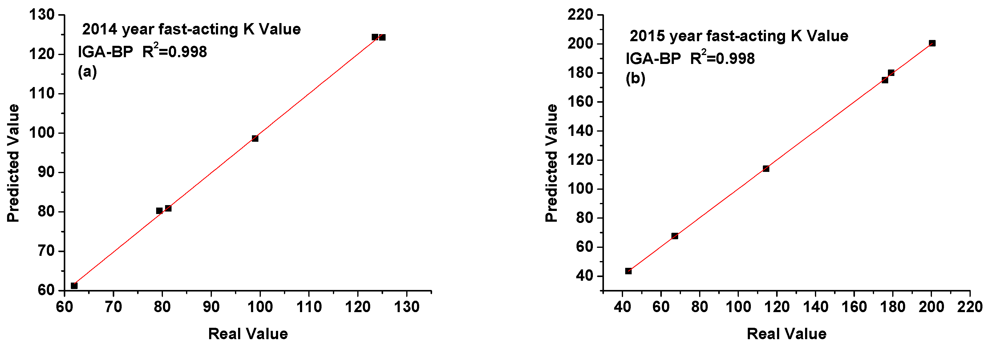
3.5. Time Series Prediction of Fast-Acting Potassium Value in Soil

Total nitrogen, organic matter, pH, available phosphorus, available iron, available manganese, available copper, and available zinc were used as input, while the value of fast-acting potassium was used as the output.

The fast-acting potassium value in soil predicted using the IGA–BP neural network showed that the correlation R² was over 0.99 in 2014 and 2015 as shown in Figure 8. Simultaneously, the RMSEs of the prediction results in

Table 5. Prediction results of fast-acting potassium value in soil.

Soil Nutrients	Township Name	Year 2014				Year 2015
		Actual Value	IGA–BP	GA–BP	BP	Actual Value	IGA–BP	GA–BP	BP
Fast-acting potassium (mg/kg)	Zhufeng Street	99.00	98.61	97.63	94.63	175.94	175.02	176.08	179.96
	Gangkou Town	81.25	80.91	80.46	77.47	114.36	114.00	113.88	116.86
	Jialu Town	123.50	124.38	125.39	127.94	179.20	180.17	180.69	178.44
	Wangxi Street	62.00	61.26	63.65	62.86	43.10	43.50	44.73	45.82
	Xiaxi Town	125.00	124.30	124.77	123.12	200.48	200.57	199.55	196.80
	Zhongxi Town	79.40	80.27	77.61	82.55	67.11	67.71	66.76	63.02
	MSE		0.474	1.999	11.229	MSE	0.409	1.017	10.110
	RMSE		0.688	1.414	3.351	RMSE	0.640	1.008	3.179

for two consecutive years were reduced by a factor of five for the BP models and by a factor of two for the GA–BP models. The maximum relative error values of the IGA–BP and GA–BP models in 2015 were 0.92% and 3.77%, respectively. The prediction accuracy of fast-acting potassium was considerably improved, providing data support for the precise fertilization of soil crops.

3.6. Time Series Prediction of Available Phosphorus Value in Soil

Total nitrogen, organic matter, pH, fast-acting potassium, available iron, available manganese, available copper, and available zinc were used as input, while the value of available phosphorus was used as the output.

The prediction correlation R² for available phosphorus of the IGA–BP neural network was 0.998 in 2014 and 0.989 in 2015 as shown in Figure 9, indicating that the accuracy of the prediction results was extremely high. The RMSEs of the prediction results in

Table 6. Predicted values of available phosphorus in soil.

Soil Nutrients	Township Name	Year 2014				Year 2015
		Actual Value	IGA–BP	GA–BP	BP	Actual Value	IGA–BP	GA–BP	BP
Available phosphorus (mg/kg)	Zhufeng Street	12.60	13.38	12.64	13.46	17.20	17.45	17.57	16.99
	Gangkou Town	5.53	5.20	6.28	5.85	7.55	8.24	8.00	8.25
	Jialu Town	2.40	2.43	2.41	3.27	6.50	6.93	6.22	7.29
	Wangxi Street	19.60	19.61	19.21	19.76	14.20	13.78	13.65	15.15
	Xiaxi Town	29.70	29.65	30.52	30.48	8.60	8.60	9.17	9.45
	Zhongxi Town	16.36	16.28	17.13	14.79	7.17	6.96	6.57	7.82
	MSE		0.122	0.331	0.783	MSE	0.159	0.233	0.536
	RMSE		0.349	0.576	0.885	RMSE	0.398	0.483	0.732

for the two consecutive years decreased by a factor of 2 for the BP models and by a factor of 1.5 for the GA–BP models. The mean relative error values of the IGA–BP and GA–BP models in 2015 were 3.86% and 5.21%, respectively. The prediction results of fast-acting potassium and available phosphorus in soil were good because fast-acting potassium and available phosphorus were the nutrients present in soil. Thus, they were closely related to the available nutrients in soil in the input, increasing the accuracy of the model.

4. Conclusions

In this study, GA was improved to optimize a BP neural network structure, the threshold values of neurons in the hidden layer, and connection weights. Next, this IGA was used to predict the soil nutrient time series. The predicted pH value, total nitrogen, organic matter, fast-acting potassium, and effective phosphorus components in soil nutrients were obtained on the basis of the BP, GA–BP, and IGA–BP neural network models. The experimental results showed that the coefficients of determination (R²) of the total nitrogen, organic matter, fast-acting potassium, and effective phosphorus in soil on the basis of the IGA–BP neural network model were all greater than 0.98. However, the R² of pH value was only 0.8 because soil pH was related to various components in soil. Although only six points are shown in from Figure 5 to Figure 9, these points were representative, and our experimental results were good. Overall, the IGA–BP neural network model exhibited better prediction accuracy and generalization ability. It can accurately predict soil nutrient content and considerably reduce soil testing costs. Meanwhile, production costs can be decreased and production yields can be increased through the precise fertilization of crops. Simultaneously, soil ecological environment can be effectively protected. Furthermore, we hope to obtain soil nutrient data from recent years through coordinated communication to further validate the validity of the model developed in this study, which is the focus of our next study.

References

1. Tian, S.; Zhang, D. Improving soil fertility and building sustainable agriculture. Tu Rang Fei Liao 2016, 5, 110. [Google Scholar]
2. Fang, X.; Li, J. Precision agriculture: Development benefits, international experience and China’s practice. Agric. Econ. 2018, 11, 28–37. [Google Scholar]
3. Jahn, B.R.; Linker, R.; Upadhyaya, S.K.; Shaviv, A.; Slaughter, D.C.; Shmulevich, I. Mid-infrared spectroscopic determination of soil nitrate content. J. Biosyst. Eng. 2006, 94, 505–515. [Google Scholar] [CrossRef]
4. Wang, T.; Wang, G.; An, Y. Design of soil nutrient content prediction model based on big data statistics. Mod. Electron. Tech. 2020, 43, 4. [Google Scholar]
5. Chlingaryan, A.; Sukkarieh, S.; Whelan, B. Machine learning approaches for crop yield prediction and nitrogen status estimation in precision agriculture: A review. Comput. Electron. Agric. 2018, 151, 61–69. [Google Scholar] [CrossRef]
6. Liakos, K.; Busato, P.; Moshou, D.; Pearson, S.; Bochtis, D. Machine learning in agriculture: A review. Sensors 2018, 18, 2674. [Google Scholar] [CrossRef] [PubMed] [Green Version]
7. Shi, P.; Wang, Y.; Xu, J.; Zhao, Y.; Yang, B.; Yuan, Z.; Sun, Q. Rice nitrogen nutrition estimation with RGB images and machine learning methods. Comput. Electron. Agric. 2021, 180, 105860. [Google Scholar] [CrossRef]
8. Zha, H.; Miao, Y.; Wang, T.; Li, Y.; Zhang, J.; Sun, W.; Feng, Z.; Kusnierek, K. Improving unmanned aerial vehicle remote sensing-based rice nitrogen nutrition index prediction with machine learning. Remote Sens. 2020, 12, 125. [Google Scholar] [CrossRef] [Green Version]
9. Hengl, T.; Leenaars, J.G.B.; Shepherd, K.D.; Walsh, M.G.; Heuvelink, G.B.M.; Mamo, T.; Tilahun, H.; Berkhout, E.; Cooper, M.; Fegraus, E. Soil nutrient maps of sub-saharan africa: Assessment of soil nutrient content at 250 m spatial resolution using machine learning. Nutr. Cycl. Agroecosyst. 2017, 109, 77–102. [Google Scholar] [CrossRef] [Green Version]
10. Saeedi, E.; Hossain, M.S.; Kong, Y. Feed-forward back-propagation neural networks in side-channel information characterization. J. Circuits Syst. Comput. 2019, 28, 1950003. [Google Scholar] [CrossRef]
11. Andriyanov, N. Methods for preventing visual attacks in convolutional neural networks based on data discard and dimensionality reduction. Appl. Sci. 2021, 11, 5235. [Google Scholar] [CrossRef]
12. Li, Z.; Shi, K.; Dey, N.; Ashour, A.S.; Wang, D.; Balas, V.E.; McCauley, P.; Shi, F. Rule-based back propagation neural networks for various precision rough set presented KANSEI knowledge prediction: A case study on shoe product form features extraction. Neural Comput. Appl. 2017, 28, 613–630. [Google Scholar] [CrossRef]
13. Zeng, Y.; Zeng, Y.; Choi, B.; Wang, L. Multifactor-influenced energy consumption forecasting using enhanced back-propagation neural network. Energy 2017, 127, 381–396. [Google Scholar] [CrossRef]
14. Kim, M.; Gilley, J.E. Artificial neural network estimation of soil erosion and nutrient concentrations in runoff from land application areas. Comput. Electron. Agric. 2008, 64, 268–275. [Google Scholar] [CrossRef] [Green Version]
15. Cross, M.; Eller, A.; Qadi, A. Estimating terrain parameters for a rigid wheeled rover using neural networks. J. Terrach 2013, 50, 165–174. [Google Scholar] [CrossRef]
16. Adeyemi, O.; Grove, I.; Peets, S.; Domun, Y.; Norton, T. Dynamic neural network modelling of soil moisture content for predictive irrigation scheduling. Sensors 2018, 18, 3408. [Google Scholar] [CrossRef] [Green Version]
17. Li, X.; Wang, J.; Ma, Y.; Lin, P.; Zhang, Y.; Wang, Z.Y. Research on soil moisture forecast model based on BP neural network-a case study at feidong county. Chin. J. Soil Sci. 2017, 48, 292–297. [Google Scholar]
18. Liu, D.; Liang, G.; Zhou, W.; Wang, X.; Xia, W. Fuzzy comprehensive fertility evaluation based on BP artificial network. J. Chin. Soil Fertil. 2011, 5, 12–19. [Google Scholar]
19. Li, Z.; Jing, Z.; Pei, D.; Zhao, Y.; Bo, P. An SA–GA–BP neural network-based color correction algorithm for TCM tongue images. Neuro Comput. 2014, 134, 111–116. [Google Scholar]
20. Shcn, Y.; Ceng, W.; Ou, M.; Kuang, Y. Forecast of amount of farmland irrigation based on BP neutral network. J. Agric. Mech. Res. 2015, 37, 36–39. [Google Scholar]
21. Beyki, M.; Yaghoobi, M. Chaotic logic gate: A new approach in set and design by genetic algorithm. Chaos Solitons Fractals 2015, 77, 247–252. [Google Scholar] [CrossRef]
22. Zheng, F.; Zeng, L.; Lu, Y.; Kai, G.; Fu, S. Fault diagnosis research for servo valve based on GA-BP neural network. J. Comput. Theor. Nanosci. 2015, 12, 2846–2850. [Google Scholar] [CrossRef]
23. Ning, L.; Qi, Z.; Fuxing, Y.; Deng, Z. Research of adaptive genetic neural network algorithm in soil moisture prediction. Comput. Eng. Appl. 2018, 54, 54–59. [Google Scholar]
24. Dong, M.; Wang, C.; Li, B.; Tang, D.; Song, W. Study on soil available zinc with GA-RBF neural network based spatial interpolation method. Acta Pedol. Sin. 2010, 47, 42–50. [Google Scholar]
25. Meng, Z.; Long, X.; Gai, H.; Dang, Z.L.; Wang, S.; Xu, P. Identification of the shear parameters for lunar regolith based on a GA-BP neural network. J. Terramechanics 2020, 89, 22–29. [Google Scholar]
26. Zhang, X.; Gao, M. Water quality prediction method based on IGA-BP. Chin. J. Environ. Eng. 2016, 10, 1566–1571. [Google Scholar]
27. Zhang, F.; Zhang, X.; Chen, L.; Sun, L.; Zhan, W. Binocular camera calibration using improved genetic algorithm to optimize neural network. China Mech. Eng. 2021, 32, 1423–1431. [Google Scholar]
28. Jian, G.; Yin, G.; Huang, P.; Guo, J.; Chen, L. An improved back propagation neural network prediction model for subsurface drip irrigation system. Comput. Electr. Eng. 2017, 60, 58–65. [Google Scholar]
Figure 1. Distribution of sampling points.
Symmetry 15 00151 g001
Figure 2. Parameter encoding method.
Symmetry 15 00151 g002
Figure 3. Flowchart of the IGA–BP algorithm.
Symmetry 15 00151 g003
Figure 4. Generation of fitness change curve.
Symmetry 15 00151 g004
Figure 5. Prediction results of the pH value in soil by using the IGA–BP neural network in (a) year 2014 and (b) year 2015.
Symmetry 15 00151 g005
Figure 6. Prediction results of the total nitrogen value in soil by using the IGA–BP neural network: (a) year 2014 and (b) year 2015.
Symmetry 15 00151 g006
Figure 7. Prediction results of the soil organic matter value in soil by using the IGA–BP neural network: (a) year 2014 and (b) year 2015.
Symmetry 15 00151 g007
Figure 8. Prediction results of the fast-acting potassium value in soil by using the IGA–BP neural network: (a) year 2014 and (b) year 2015.
Symmetry 15 00151 g008
Figure 9. Available phosphorus value predicted using the IGA–BP neural network: (a) year 2014 and (b) year 2015.
Symmetry 15 00151 g009