Article

Determination of Air Traffic Complexity Most Influential Parameters Based on Machine Learning Models

by
Francisco Pérez Moreno
1,*,
Víctor Fernando Gómez Comendador
1,
Raquel Delgado-Aguilera Jurado
1,
María Zamarreño Suárez
1,
Dominik Janisch
2 and
Rosa María Arnaldo Valdés
1
1
Department of Aerospace Systems, Air Transport and Airports, Universidad Politécnica de Madrid (UPM), 8040 Madrid, Spain
2
ATM Research and Development Reference Centre (CRIDA), 28022 Madrid, Spain
*
Author to whom correspondence should be addressed.
Symmetry 2022, 14(12), 2629; https://doi.org/10.3390/sym14122629
Submission received: 3 November 2022 / Revised: 17 November 2022 / Accepted: 8 December 2022 / Published: 12 December 2022
(This article belongs to the Special Issue Machine Learning and Data Analysis)

Abstract

:
Today, aircraft demand is exceeding the capacity of the Air Traffic Control (ATC) system. As a result, airspace is becoming a very complex environment to control. The complexity of airspace is thus closely related to the workload of controllers and is a topic of great interest. The major concern is that variables that are related to complexity are currently recognised, but there is still a debate about how to define complexity. This paper attempts to define which variables determine airspace complexity. To do so, a novel methodology based on the use of machine learning models is used. In this way, it tries to overcome one of the main disadvantages of the current complexity models: the subjectivity of the models based on expert opinion. This study has determined that the main indicator that defines complexity is the number of aircraft in the sector, together with the occupancy of the traffic flows and the vertical distribution of aircraft. This research can help numerous studies on both air traffic complexity assessment and Air Traffic Controller (ATCO) workload studies. This model can also help to study the behaviour of air traffic and to verify that there is symmetry in structure and the origin of the complexity in the different ATC sectors. This would have a great benefit on ATM, as it would allow progress to be made in solving the existing capacity problem.

1. Introduction

The Air Traffic Management (ATM) system’s main role is to ensure the safe and efficient transport of passengers and goods [1]. Modern aviation is facing a major challenge, namely the increase in demand for aircraft. In recent years, aircraft demand has increased by 3–6% per year, and EUROCONTROL estimates that it will continue to increase by 2% per year until 2025 [2]. This increase in aircraft demand exceeds the capacity of the ATM system, and this imbalance is among the main reasons for delays and congestion in air traffic [3]. Specifically, the capacity of an ATC sector is measured as the maximum number of aircraft that can cross the sector in a given time [4]. Capacity is therefore affected by many uncontrollable factors, such as the weather and actions or experience of the controllers. This makes capacity difficult to increase [5]. For this reason, the imbalance between capacity and demand is a difficult problem to solve.
According to ICAO forecasts, the current situation makes airspace very complex for the (ATC) system and this will remain so in the future. This situation is important because the Air Traffic Control system is responsible for the safe and efficient management of air traffic flows [6]. Among the current concerns of the ATM system is to reduce airspace complexity. The reason for wanting to reduce airspace complexity is that the complexity and congestion of ATC sectors are closely related to the workload of (ATCOs) [7]. It is, indeed, natural to assess the workload of ATCOs through airspace complexity, as it is independent of the human factor and this relationship is very valuable to be researched [8]. However, what is airspace complexity? It is clear that complexity is an area of concern because of its effects on traffic and ATCOs. However, there is currently no consensus on how to define complexity [9]. There are multiple metrics of complexity, most of them agreeing that air traffic complexity is a complex measure dependent on several factors and their relationships, but there is also a need for new complexity metrics [10]. A very generalised and comprehensive complexity indicator is dynamic density (DD) [11]. This indicator, or its variants, is still widely used today [12,13]. This indicator is based on a weighted sum of different variables. Although it is a widely used indicator and it has been the source of many subsequent indicators of complexity, it is considered to have a limitation. As this indicator is based on the conflicts generated in the airspace, as well as on traffic indicators, it is indirectly based on the actions of the ATCOs. This means that this indicator is also influenced by human performance.
This uncertainty in the definition of complexity, coupled with its direct relationship to the workload of controllers, means that this topic has received a considerable amount of interest from researchers around the world in recent years [14,15,16]. Although there are discrepancies in the definition of complexity, different authors agree on certain aspects. The authors think that air traffic density, in particular the number of aircraft, is the indicator that best expresses complexity. However, this parameter alone does not adequately reflect the workload of ATCOs [17]. Therefore, these authors also express the need to use other variables such as interactions between aircraft or changes in direction or speed [18]. These factors that determine the complexity of air traffic, and therefore of airspace, are of a very different nature. For this reason, interest has arisen in finding out which of the aspects mentioned in the literature are important or not, to unify the efforts made and help arrive at a complexity indicator that could be used independently of the disparate characteristics of the ATC sectors. An attempt is therefore made to arrive at an indicator that is based exclusively on air traffic characteristics.
With this in mind, this paper aims to determine which variables are really important in the determination of complexity, independently of human performance. With this objective in mind, an attempt will be made to answer the following research question: What are the variables that really determine the complexity of airspace? Throughout this paper, the methodology necessary to try to answer this question will be developed. It will be tested. At the end of the results, a reflection will be added in case this question can be answered.
The approach of this paper is novel. The model developed is based on real operational data and through the application of Big Data analysis and machine learning algorithms.
In this case, the data themselves determined in this methodology which variables are most important in determining the complexity of the airspace.
This methodology was used to identify which variables are most important in determining the complexity of airspace. For this purpose, it was based on a dynamic feature weights selection [19,20]. This approach is novel and useful, as it overcomes one of the major limitations of current complexity models. This limitation is the dependence of the models on the opinion of the ATCOs, which is subject to their bias [21]. Although the starting point of the model is, in this paper, expert opinion, this methodology should lead to the same results regardless of the initial values of the model. Therefore, the approach followed in this paper has the following advantages:
  • Determination of the most important variables in an objective way, using artificial intelligence applications. Dynamic feature weight selection made it possible to identify which variables are more important in the complexity definition, without being based on human bias.
  • Possibility of capturing different behaviours and trends, due to the different nature of the ATC sectors. This is also possible thanks to the application of machine learning algorithms.
  • Ability to adapt and capture changes in results over time as new operational data are added to the model.
Thanks to all these advantages offered by a methodology that allows obtaining which variables are more important in the determination of the complexity of airspace, it is intended to help define a complexity indicator. Although this indicator should be composed of a static series of variables to be a consistent indicator, their relative importance should be able to vary dynamically and automatically depending on the sector and the time horizon analysed. In this way, this supposed indicator could adapt to the situation analysed.
This methodology is based on feature selection [22] to develop a machine learning model based on the application of Big Data analysis [23]. The dynamic feature selection is made through the function Gini [24]. Although both Gini and Entropy are supposed to work well in this situation, Gini has been selected because it works properly in research related to this topic [25], where classification models with the random forest algorithm were developed. This model made it possible to study the behaviour of air traffic and to draw conclusions such as whether its structure and the origin of its complexity are indeed symmetrical in ATC sectors of different natures.
To show the methodology followed in this paper to determine which variables are most important to determine airspace complexity, Section 2 shows the methodology followed. Section 3 shows the results obtained with a real application. Section 4 shows the conclusions obtained in the definition of the methodology and its application and the future steps for its improvement.

2. Materials and Methods

This section presents the methodology proposed to detect which variables are the most important in the determination of airspace complexity. This methodology is divided into two main areas.
  • Definition of complexity: To be able to estimate the variables that make the airspace more complex, it is first necessary to define what complexity is.
  • Identification of the most important variables: Once the complexity has been defined, it is appropriate to identify which variables are the most influential.
The complete methodology is developed below.

2.1. Complexity Definition

The first step in determining which variables are most important for understanding sector complexity is to define what sector complexity is.
Many studies currently exist that attempt to estimate the complexity of airspace, many of them using artificial intelligence [26,27,28]. Of interest within these models are models that define airspace complexity in terms of a few simple indicators [29]. In particular, the methodology presented in [30] was the basis for the methodology of this paper. This methodology is based on the determination of complexity from the behaviour of air traffic flows within the sector. This methodology proposes the classification of air traffic flows through a variable called “impact” and the classification of ATC sectors through a variable called “complexity”, this classification is supported by machine learning models.
This methodology has the advantage of defining complexity in terms of simple statistical variables. However, this selected methodology has certain limitations that were resolved before the implementation of the methodology for selecting the most important variables.
Specifically, the complexity of an ATC sector depends on the behaviour of its aircraft, represented in this case through air traffic flows. However, it also depends on the structural aspects of the sector [31]. This last aspect is not explicitly included in this methodology. For this reason, an attempt was made to add this dimension to the selected methodology through three additional variables. These variables have been added through the review of [32,33]. It is important to note that although these three variables have been based on these references, the scope of this paper is different from the one in [32,33], having a significant contribution. In [33], the paper models the determination of airspace complexity through critical factors and genetic algorithms. In this case, a methodology based on it has been developed, but the focus of this paper goes beyond the development of the methodology. The intention of this paper is to find out which factors are critical in determining airspace complexity. The development of the methodology, while necessary, is simply a means to fulfil the real objective of this paper. In [32], a methodology for determining complexity is also proposed. This paper is also based on the work done in this reference. In addition, in this reference, there are also studies of causalities in Bayesian networks. However, in [32], a very complete model has been developed, but in which the opinion of experts is very present, which is exactly what we want to eliminate in this paper. The aim of this paper is to determine the most influential factors independently of expert opinion, for which machine learning models are used. However, in order to improve the methodology for determining the complexity, the subsequent selection of important parameters has been the basis. Additionally, the variables in Table 1 and Table 2 are based on these references but are different. This results in a different methodology from the one proposed in these two papers.
The three variables added are:
  • Mix of aircraft wake turbulence categories in the sector: Aircraft mix is traffic dependent but is considered within the structural aspects of the sector as this will vary depending on the geographical location and the type of operations and routes within the sector. For this reason, it has been considered a structural aspect of the sector.
  • Number of entry and exit points: The number of aircraft entry and exit points is a structural aspect of the sector which gives an idea of the complexity of traffic within the sector. If there are many points, the operation will be more complex.
  • Distance between entry and exit points: It is not only the number of points that is important, but also their concentration. If the points are further apart, the operation in the ATC sector will be more uniform and simpler than if the points are concentrated in certain areas of the sector.
With the incorporation of these three variables into the proposed methodology in [30] the characterisation methodology is completed. This methodology is proposed to study the complexity of the sectors from the behaviour of their air traffic flows (based on the behaviour of individual aircraft) but also on the structural aspects of the sector itself. Furthermore, it is important to note that the influence of machine learning models has been removed from this methodology, as it is considered that for the scope of this paper, machine learning models were used for another purpose. The characterisation methodology is presented in Figure 1.
This methodology is therefore the proposed methodology for defining complexity in the airspace. This methodology defines both the complexity of ATC sectors and the impact of air traffic flows daily. This methodology is based on statistical variables obtained from individual operations in the sector over time. For a better interpretation of the complexity definition methodology, these variables have been divided into four different areas [30]:
  • Air traffic density: Traffic density is the variable most closely related to complexity in the literature. For this reason, it is the first area to be considered and its importance is expected to be high.
  • Vertical air traffic density: To know the complexity of airspace, it is also necessary to know how aircraft occupy this airspace vertically. The distribution of aircraft per FLs is also a variable that is widely considered in the literature.
  • Time Distribution: This field studies the percentage of hours and days that the flows were open. This area may also be of interest.
  • ATFCM Regulations: Regulations appear when the capacity of the ATC system cannot cope with the aircraft demand. For this reason, regulations will appear in the most complex airspaces. The relationship between these regulations and complexity may also be of great interest.
The variables inside each of the areas are calculated as:
  • Daily number of Aircraft in the air traffic flow: As the air traffic flow is data provided by the CRIDA company, and the exact time of entry and exit to the sector is also available, a count of aircraft belonging to each flow is made each day.
  • Hourly number of Aircraft in the air traffic flow: As for the previous variable, it is easy to perform a count of aircraft entering the sector by a concrete flow each hour. To maintain the daily time horizon, all hourly counts on the same day are averaged.
  • Maximum aircraft in an hour in the air traffic flow: Starting from the hourly counts of a given day for each flow, the maximum of the sample is taken. This is taken because the peak hourly traffic is just as important as the average hourly traffic.
  • Percentage of changing FL Aircraft in the air traffic flow: Information on the average flight level of all aircraft, and the standard deviation is taken. If the standard deviation of the FL is different from zero, it is because the aircraft has changed FL at some point. All aircraft with a standard deviation of FL different from 0 are divided by the total number of aircraft each day.
  • Number of Ascending/Descending aircraft in the air traffic flow: Data are available for the vertical speed of aircraft in the sector. If this vertical speed is other than 0, the aircraft is ascending/descending. The ascents and descents are combined because one case is equally complex for the ATCOs as the other. To obtain this variable, a count is made of all aircraft per day and per flow that have a vertical speed different from 0.
  • Number of Cruise aircraft in the air traffic flow: Complementary to the previous variable, this variable is obtained by counting all aircraft per day and per flow that have a vertical speed of 0.
  • Number of Occupied FL in the air traffic flow: Information is available on the flight levels of the aircraft within each sector. Information is also available on the flows to which each aircraft belongs. With this, a count is made of the different flight levels that appear each day in the flow. This variable will be the total number of different flight levels.
  • Number of Aircraft per FL in the air traffic flow: With the above information, it is also easy to make a count of how many aircraft are in each flight level per flow per day. With the number of aircraft in each flight level, an arithmetic mean is made.
  • Days that the air traffic flow is occupied within a year: A flow does not necessarily have aircraft every day of the year. With the information on the entry and exit of the aircraft sector of each flow, the day of entry is considered. This is used to calculate which days there will be aircraft and which days there will not. The number of days on which there will be aircraft is divided by 365 to give the percentage. These data will be unique for each flow during the whole period, contrary to the rest of the parameters, but are still considered as they give very useful information.
  • Hours that the air traffic flow is occupied within a day: Like the previous variable, the time of the entry of the aircraft is used, and the flow to which they belong. In this case, the specific time is considered, and a count is made of the hours during which the flow will have aircraft. The total of these hours is calculated and divided by 24 to make the percentage.
  • Percentage of regulated aircraft in the air traffic flow: Another piece of information is the number of regulations affecting each flight. All those aircraft in the flow each day with a non-zero number of regulations have been divided by the total number of aircraft in the flow on that day.
  • Mean regulations in the air traffic flow: Of all aircraft in each flow on the analysis day, the arithmetic means of the regulations are calculated.
  • Mean regulations based on regulated aircraft in the air traffic flow: Of all aircraft with several regulations greater than zero (regulated aircraft) in each flow on the analysis day, the arithmetic mean of the regulations is calculated. This variable is also considered because the meaning is different from the previous variable. It is not the same to see which regulations affect on average, being strongly influenced by unregulated aircraft, as it is to see the average regulations only when knowing that they are regulated.
  • Percentage of delayed aircraft in the air traffic flow: This is also available for each aircraft. The number of aircraft with a delay greater than zero on a day in a flow is divided by the number of total aircraft on that day in that flow.
  • Mean delay in the air traffic flow: From all aircraft in each flow on the analysis day, the arithmetic mean delay is calculated.
  • Mean delay based on regulated aircraft in the air traffic flow: From all regulated aircraft in each flow on the analysis day, the arithmetic mean of the delay is calculated.
Mean delay based on delayed aircraft in the air traffic flow: Of all aircraft with a delay greater than zero (delayed aircraft) in each flow on the analysis day, the arithmetic mean of the delay is calculated.
These statistical variables were rescaled between 0 and 1 (where 0 is the minimum and 1 is the maximum of the variable for all air traffic flows in the period considered) so that some variables do not stand out over others throughout the methodology.
To achieve better comprehension of the methodology, and of the subsequent machine learning models implemented, all the statistical variables studied are presented in Table 1, divided into the four areas described. Furthermore, to improve the reproducibility of the methodology, an example of a real case of the variables is presented in Table 1 in brackets to better understand the format of the data.
With these variables, mean values and coefficients of variation were calculated. Additionally, with these values, the variables called mean impact and impact variability were calculated using weighted sums (see [30]). The mean impact and impact variability were later re-scaled between values 1 and 5. These variables were calculated daily, which results in a methodology that defines complexity daily. In the example data shown in Table 1, the mean impact is 3.69 and the impact variability is 1.68.
The next stage of the methodology is the definition of the impact of air traffic flows. This is defined from the mean impact and impact variability by using a table model. This table model is presented in Figure 2.
This model table is based on a risk matrix [34,35]. In these matrices, the risk tier of the impact and the probability of occurrence are assessed. In these matrices, the two variables are discretised from 1 to 5 and a discretised risk from 1 to 5 will also be obtained. In this model table, the axes will be the average impact and the variability of the impact. These two variables will also be discretised from 1 to 5, resulting in 5 impact tiers. Tier 1 is green, and tier 5 is dark red. The distribution of impact tiers has been done employing expert opinion with staff from Enaire, CRIDA and Universidad Politécnica de Madrid.
Although the mean impact and impact variability are continuous variables, they are discretised for this table model. In the case of the example, they would change from 3.69 and 1.68 to 4 and 2, respectively. These two values are combined in the table model, and result in an impact of 5.
At this point, the variable impact has already been defined. This variable is fundamental to the model as it allows the behaviour of flows to be studied. The behaviour of the flows, together with the newly added structural aspects, constitute the complexity of the ATC sectors.
Table 2 presents the variables used in the definition of complexity, divided into those that form the flow parameter and those that form the sector parameter. As stated before, the main addition of this methodology from the one in [30] is the sector parameter variables. These variables and the flow parameter variables were calculated daily as we are defining a methodology that calculates the complexity of the ATC sectors daily. These variables are calculated as:
  • Number of air traffic flows in the ATC sector: The number of flows into which the airspace is distributed is provided by CRIDA.
  • Percentage of air traffic flows with 5-level impact: Of the total flows present in the airspace on the day of analysis, the impact is calculated as described above. The number of flows with 5-level impact is divided by the total number of flows.
  • Distribution of wake turbulence categories in the ATC sector: The most complex situation for the ATC service is that there is an equal number of aircraft of the different wake turbulence categories. The simplest situation is when all aircraft are in the same wake turbulence category. Therefore, the most complex situation will be 5 of the overall variables, and the simplest will be 1. The percentage of aircraft in each wake turbulence category is therefore calculated on the day of operation, and the deviation from these two extremes is measured.
  • Number of points where Aircraft enter/exit the ATC sector: All air traffic flows will have a sector entry and exit point. However, the entry or exit points of several flows may coincide. Therefore, the number of entry or exit points may be 2·number of flows or less. The number of entry or exit points is calculated and divided by (2·number of flows). This will result in a parameter between 0 and 1.
  • Distance between points where Aircraft enter/exit the ATC sector: The distance in km between the different entry or exit points is calculated. The arithmetic mean is then calculated.
These variables are rescaled directly between 1 and 5 using as limits for each variable its maximum and minimum over the whole period studied. In Table 2, a real data example is presented in brackets to show the format of the data.
The flow parameter and the new sector parameter are defined with weighted sums of their parameters, and then the complexity is defined using a table model similar to Figure 2. The flow parameter can be paralleled with the mean impact, and the sector parameter with the impact variability to define the complexity table model. In the proposed example, the flow parameter is 2.55 and the sector parameter is 2.16. This results in a complexity of 3.
With this last step, the methodology to assess the complexity of airspace based on the methodology proposed in [30] is fully defined. This methodology is therefore able to define both the impact of an air traffic flow and the complexity of the airspace, depending on several different characteristics. This model has been chosen because of several advantages:
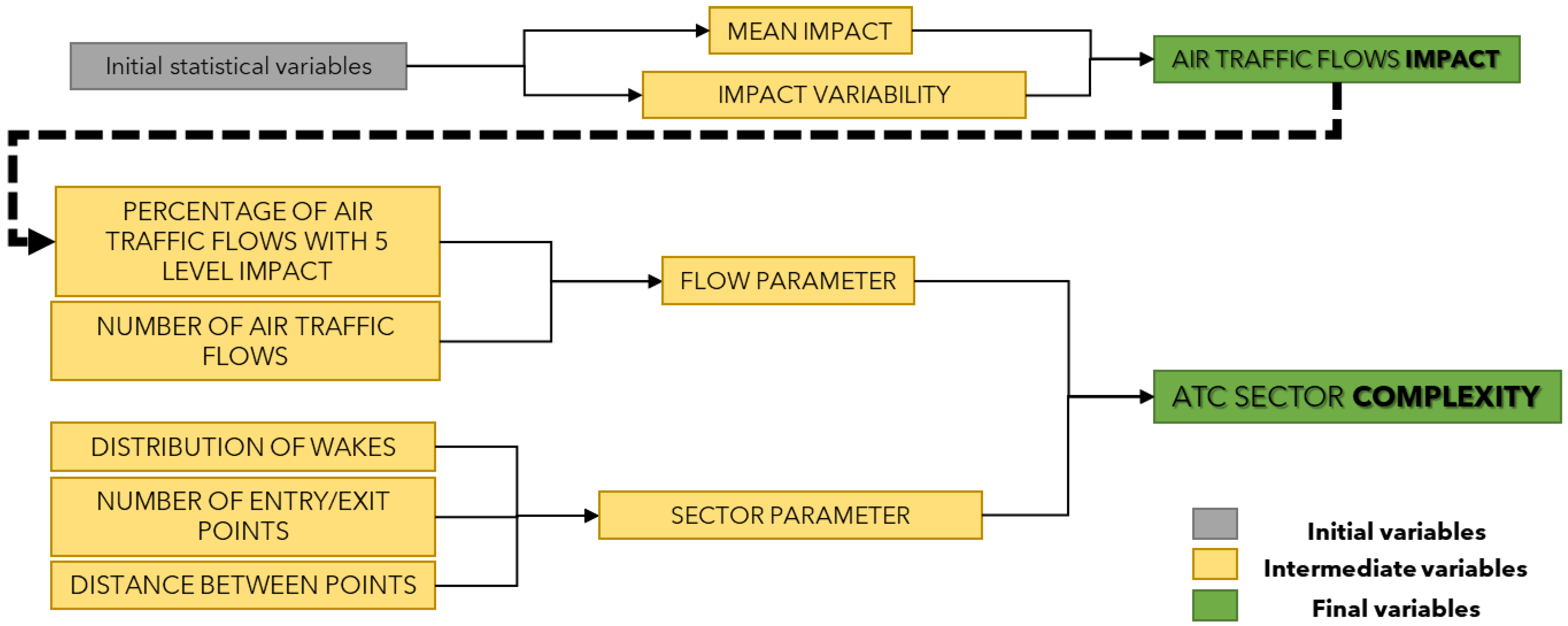
  • The model determines the impact of flows, and the complexity of the sector, based on simple statistical variables. These variables are representative.
  • The division of the variables is accurate and based on a correct analysis of the literature.
  • The definition of impact and complexity is based on weighted sums, which is good for a machine learning model to obtain relative importance and be representative.
It has been identified how the complexity of the sectors was defined. The next step was to define how to come up with a model that allows us to say which variables are most important in determining complexity.

2.2. Most Important Variables Identification

Once a model has been identified with which complexity can be determined based on several simple statistical variables, it is necessary to determine which variables are the most important. A machine learning model is used for this purpose. The major advantage of using a machine learning model is that the results obtained are the product of the patterns present in the data, rather than the bias of the experts.
Even if in this case expert opinion is used as a starting point. Expert opinion is only a necessary starting point for the methodology. To test that the methodology leads to the same results independently of expert opinion, the starting point of the methodology has been arbitrarily varied. As the results obtained were similar, it can be justified that the methodology eliminates the expert bias.
Even so, this expert opinion is the most operationally meaningful starting point. This will later be used to compare it with the results obtained. Moreover, this good starting point served to accelerate the convergence of the algorithm. For these reasons, expert opinion is used as a starting point in this paper.
In this paper, two machine learning models were determined. The first model determined the impact of air traffic flows. The first model determined the complexity of the ATC sectors. This division was based on the fact that the distribution of flows is a fundamental indicator of complexity [36], and that in this model it is represented by the impact of the air traffic flows. The function of machine learning models was not to predict the output, as in most machine learning for ATM [28,37]. In this case, the objective is to analyse the relative importance of the input variables. A wide variety of algorithms are used in industry for machine learning models [38]. There are algorithms based on decision trees such as the random forest algorithm or the logistic tree classifier. There are also other families of classifiers such as ree, Perceptron, Lazy, Bayes, SVM, Regressions and ANN [39].
In this case, a random forest algorithm was, therefore, used for both these models, as it works properly in different nature problems [40,41], and it is also easy to extract relative importance with decision tree-based algorithms [42]. This relative importance analysis was the key to finding out which variables are the most influential in determining impact and complexity. This relative importance extraction was based on the feature importance method [43].
As the determination of impact and complexity is based on weighted sums, the result will change if the weights of these sums change. Thus, the relative weights obtained by the machine learning model were considered the new weighted sum weights, so that the model is mainly influenced by the machine learning algorithm rather than by the bias of the experts. However, the relative weights proposed by the machine learning model may vary greatly from the initial relative weights. Therefore, it cannot be said that these are the final relative weights.
To solve this, an iterative process is implemented in which the relative importance varied until a certain stability is reached. This stability is achieved when, between one iteration and the next, none of the model’s relative importance has varied by more than 5%.
S t a b i l i t i t y   R I j i R I j i 1 < 0.05 R I j i     j
where RI is the relative importance of the j variables in iterations i and i − 1.
When the required stability is reached, the relative weights obtained remain approximately constant. It is these relative weights that will tell which variables are most important in determining both the impact of air traffic flows and the complexity of ATC sectors.
Figure 3 presents the process of obtaining the relative weights which tell which variables are most important in determining impact and complexity. The process marked in red indicates the first iteration of the loop, using the weighted sum with the weights indicated in [30], based on expert opinion. In black is marked the update loop of the relative importance, this loop is run until it reaches the final relative importance with which stability is reached. As the process is common to the two machine learning models defined, the input and output variables of the model are not specified in the process of Figure 3. It has been specified in Figure 3 that there are two models, the first to determine the impact of air traffic flows, and the second to determine the complexity of the ATC sectors.
This process is very robust and has a great advantage. The process allows obtaining, based on initial relative importance based on the bias of the experts, relative importance based mainly on the real operating data. This eliminates much of the subjectivity of the initial model.

2.3. Evaluation of Machine Learning Models

The aim of this methodology is not to predict the output of a machine learning model, but to analyse the relative importance of the variables. However, to verify that the relative importance obtained is valid, the performance of the model was evaluated in parallel. As the impact and complexity are determined in two independent models, they were also evaluated independently. In this section, the evaluation methods of the developed machine learning models are mentioned.
First, it has been decided to propose an evaluation method using the following indicators, based on [44].
The first indicator selected is accuracy. This indicator measures the total percentage of well-classified cases out of the total number of cases. The mathematical equation for this indicator is:
A c c u r a c y = T P + T N T P + T N + F P + F N
TP being True Positive elements, TN being True Negative elements, FP being False Positive elements, and FN being False Negative elements.
As the methodology operates on the assumption that the output is correct, a minimum tier of 90% accuracy is set to be able to perform an analysis of the relative importance of the variables.
Accuracy is a great indicator to measure the overall performance of the model, but three additional indicators are also presented for more detailed information [44,45]:
p r e c i s i o n = T P T P + F P
r e c a l l = T P T P + F N
F 1 -score = 2 p r e c i s i o n r e c a l l p r e c i s i o n + r e c a l l = T P T P + F N + F P 2
Recall indicates the ability of the algorithm to accurately detect when the sector will be regulated or not. The precision indicates the ability of the algorithm to detect the categories. Additionally, the F1-score is a harmonic mean of the recall and the precision [46]. The F1-score complements the precision and recall indicators. The precision indicator measures FP elements, the recall measures FN elements. Therefore, the F1-score is a measure of both FP and FN that is widely used in the evaluation of machine learning models.
These indicators should also be above 0.9 out of 1 to be considered adequate in these models.
With these four parameters, the machine learning models are evaluated. If the defined requirements were met, the models were considered correct, and the analysis of the relative importance of the variables was considered meaningful.

3. Results

Once the methodology to identify which variables are the most important in determining both the impact and the complexity of the model has been presented, the validity of this methodology is tested in a real scenario application. For this test, data from all operations in six ATC sectors in Spanish airspace during 2019 have been used.
The input data to the methodology comprise more than 3 million aircraft from different sectors. They have been obtained based on ENAIRE radar traces and have been provided to the authors after processing and validation by the company CRIDA. ENAIRE and CRIDA’s presence for the pre-filtering of the data is a great help. The data belong to radar traces, so it can be expected that there will be a lot of noise in the sample, coming from a highly noisy environment. However, thanks to ENAIRE and CRIDA, it can be assured that the data used for the development of this methodology and for its testing will be free of errors due to the noise in the sample.
Figure 4 shows the sectors where the model has been tested.
Six sectors have been chosen to try to capture the different typologies of ATC sectors in Spanish airspace.
  • Low Sectors: These sectors are sectors where aircraft are in evolution (climbing/descending) and at a low flight level (FL). These ATC sectors are the sectors immediately above the terminal maneuvering area (TMA) of the airports. Available examples of these sectors are Castejón Low (LECMCJL) and Gran Canaria Northeast (GCCCRNE).
  • Upper Sectors: These ATC sectors are occupied by aircraft flying at high FLs and in a cruising regime. There is usually much less variability in operation. They are more stable sectors. The sectors selected as a sample, in this case, are Pamplona Upper (LECMPAU) and Domingo Upper (LECMDGU).
  • Integrated Sectors: These are sectors where enroute operation is combined with arrival and departure operation. They are normally operational at night as there are fewer aircraft. As there is more variability in the operation, they are only operational when traffic is lower so that the same ATCOs can take care of the operation in cruise and evolution. The integrated sectors to be studied are Teruel Zaragoza Integrated (LECMTZI) and Toledo Integrated (LECMTLI).
This selection of sectors has been made with two main purposes in mind:
  • To assess the suitability of the methodology for sectors operating differently from each other and whether it can detect the most important variables under different operating conditions.
  • To verify whether the sectors classified in the different groups are similar in nature and whether the methodology can capture this.
The results obtained were divided into two subsections, respecting the two different machine learning models proposed in the methodology. Therefore, the results obtained from the analysis of the impact of air traffic flows and the analysis of the complexity of the ATC sectors are shown separately.

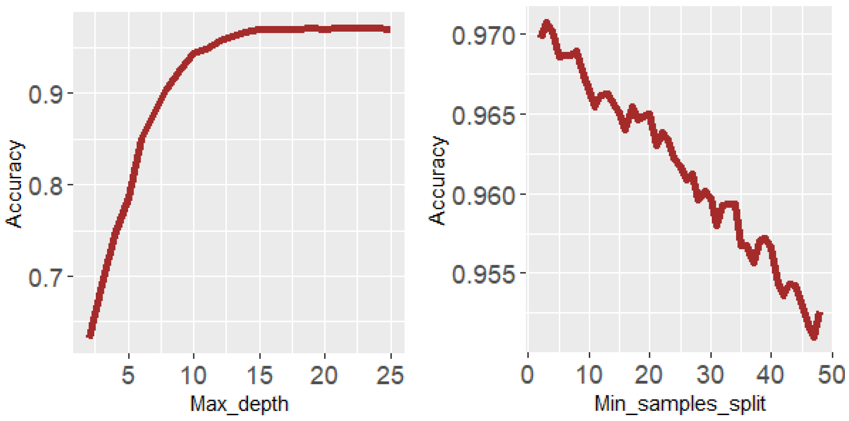
3.1. Hyperparameters of Machine Learning Models

As already mentioned, the random forest algorithm has been chosen for the development of these machine learning models, but this algorithm can be customised depending on the hyperparameters that are specified. The correct choice of the hyperparameters of the model can have a great influence on its accuracy [48]. For this reason, it was decided to analyse the hyperparameters of the machine learning models before their complete evaluation. Specifically, the hyperparameters chosen are:
  • N_estimators: Total number of trees to be constructed in the forest [49].
  • Max_features: Used for denoting the maximum number of variables used in independent trees [49].
  • Max_depth: The maximum number of times that the trees will be divided.
  • Min_samples_split: The minimum number of samples necessaries to split the branch of the tree.
It is estimated that these hyperparameters are sufficient to optimise the results of the models.
As in this methodology, the number of machine learning models applied will depend on the number of iterations until stability is reached, it is not possible to test all the models beforehand. For this reason, it has been decided to test each of the models once, optimise their hyperparameters, and leave them constant throughout the process. In particular, the impact and complexity model which relative weights correspond to expert opinion has been optimised.
Firstly, the analysis of the impact model is carried out. Plots will be shown where accuracy will be evaluated as the hyperparameters studied vary. First, in Figure 5, the influence of n_estimators and max_features are shown.
Very similar behaviour is observed for the three max_features, in which, as n_estimators increases, accuracy stabilises. It is important to consider that the graph has a lot of zoom, so the behaviour is much more stable than it seems. The final accuracy values are also very similar, although sqrt seems to perform slightly better.
The influence of max_depth and min_samples_split is then presented. This is depicted in Figure 6.
As for max_depth, behaviour stabilises at a max_depth of 15. From this point on, accuracy remains approximately constant. On the other hand, the min_samples_split decreases the accuracy as it increases. This is expected since the higher the hyperparameter, the less accurate the model will be. In order to avoid underfitting or overfitting, it has been decided to keep it at 5.
With these three plots it has been possible to study the behaviour of the machine learning model of impact. Subsequently, the specific parameters that will make up this random forest algorithm have been selected. These hyperparameters are shown in Table 3 once the complexity has been analysed.
The next model to be studied is the complexity model. To analyse its hyper-parameters, the same process is used as for the impact model. Therefore, first the influence of n_estimators and max_features is shown in Figure 7.
The hyperparameter n_estimators in this case has a much more stable behaviour from 80 trees onwards in the random forest. The max_feature log2 is not visible in Figure 7 because it has exactly the same values as sqrt. As these are slightly more stable, and for consistency with the impact model, the same values of these hyperparameters are selected.
The next analysis is that of max_depth and min_samples_split in the complexity model. This analysis is presented in Figure 8.
In this case, the behaviour of max_depth in the complexity model is analogous to the behaviour of the impact model. The parameter has no influence on accuracy at 15 and above. On the other hand, min_samples_split seems to stabilise at 25 samples and above. For this reason, this is the value chosen for this hyperparameter.
Once this analysis has been completed, we proceed to define all the hyperparameters for both models. These are listed in Table 3.
Therefore, the optimal results will be obtained with these hyperparameters. It is important to note that the models are very robust, so the results in this case will not be greatly influenced by the hyperparameters. The variation is as low as 0.01, except for very low values of max_depth where the variation is noticeable.

3.2. Evaluation of Machine Learning Models

Once the hyperparameters are defined, and before obtaining the results of the features’ relative importance. It is important to evaluate the performance of the machine learning models on which the proposed methodology is based. In this section, both the machine learning model that predicts the impact of the air traffic flows and the complexity of the ATC sectors are evaluated.
To evaluate these models, the parameters proposed in Section 2.3 are used. First, an overview of the models are given using accuracy. Subsequently, a more exhaustive analysis was carried out using the parameters of Equations (3)–(5).
The evaluation of the models has been performed using 80% of the total data for training and 20% for the test.
The first model to be evaluated is the model predicting the impact of air traffic flows, which accuracy is:
A c c u r a c y   1 = 0.97
The accuracy is above 0.95, so it satisfies the previously defined requirements. A 97% accuracy of the total number of cases tested is an almost perfect performance of the impact prediction model. The three parameters for each of the impact tiers are presented in Table 4 below.
In all cases described in Table 3, the parameters are above 0.95. This leads to a model that is both generally and specifically very reliable. In the sample analysed, there are no impact flows at level 1, so it is not shown in the table.
With these results, the impact prediction model is validated against the established criteria. The next model is the one that predicts the complexity of the ATC sectors. Firstly, their overall performance is assessed by employing accuracy.
A c c u r a c y   2 = 0.97
The accuracy of this model is again 0.97, so the previously defined criteria are met. For a better verification of the performance of the model, the parameters accuracy, recall and f1-score are presented in Table 5.
In this case, none of the ATC sectors has a complexity of 1 or 5 in the test sample. The indicators are again equal to or greater than 0.95. With this table, it can be assured that the complexity prediction model also performs very well in the scenarios studied.
With the results obtained in this section, it can be assured that the models are very accurate so that the analysis of features’ relative importance can be performed as proposed in the proposed methodology.

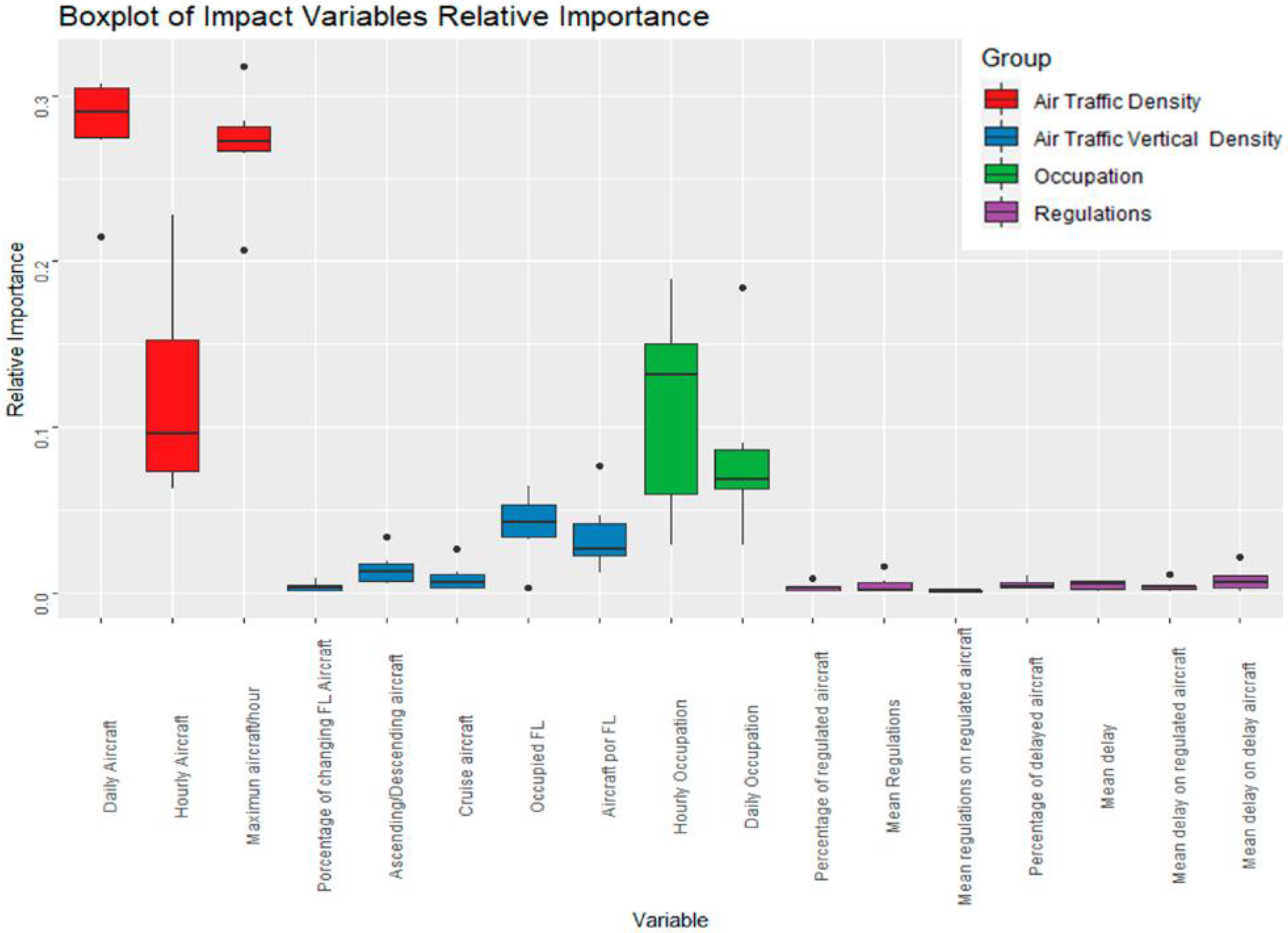
3.3. Analysis of the Impact Most Important Variables

Once the machine learning models have been proven to be correct and the predictions made are accurate, the first step in the analysis of the results is to assess which variables are most important in determining the impact of air traffic flows on the available airspace. In total, in the six sectors analysed, there is a total of 1.8 million data, which correspond to the 17 variables and the impact of the different flows identified for each of the 365 days of the year.
Despite appearing to be a complex model with 17 variables, the model is actually very simple, as it is based on the methodology described above. For this reason, it was very easy for the model to determine its prediction. The aim of this paper is not to know the output, but to study the relative weights in order to know which variables are most important. In fact, the previous analysis determined that the prediction results of the model are excellent. Moreover, the computation time for training and prediction of each model was around 45s in total. This is a minimum time. This is because the model will easily find the behavioural patterns as they are explicitly given by the methodology.
The proposed methodology has been conducted for the six ATC sectors separately to differentiate the results. To achieve stability, different iterations have been needed in each case. The higher the number of iterations needed to reach stability, the more complex the determination of the relative importance is. This makes the number of iterations important information of the model and indicates in which sector the traffic patterns are clearer. These iterations are shown in Table 6:
The number of iterations varies considerably depending on the sector of analysis. Studying their behaviour by groups, it is observed that low sectors reach convergence with a lower number of iterations, while integrated sectors need more iterations. Integrated ATC sectors combine climb/descent operation with the enroute operation, so traffic patterns are more complex. On the other hand, in the upper sectors, there is a large variability in the number of iterations. LECMDGU reaches convergence in 4 iterations, following the trend of the low sectors, which reach the required stability earlier than the integrated sectors. LECMPAU, on the other hand, reaches convergence in 12 iterations. It is estimated that this difficulty in reaching the final results is since the operation in this sector is very complex and the algorithm needs more iterations to find the traffic patterns necessary to know the relative importance of the variables that define the impact of air traffic flows.
From the proposed methodology, the data worth analysing are the final relative importance of the variables. The rest of the intermediate relative importance were simply data that the model obtained to continue the process, but they have no theoretical value. The results obtained for the different sectors, in terms of the final relative importance, are shown below. These results are shown in Figure 9. The initial relative importance, proposed by expert opinion, is also shown. The aims are to see and compare the results in each of the sectors, making a comparison between the different types of ATC sectors if possible. Another objective is to see how the relative importance has changed concerning what was proposed by expert opinion.
In all ATC sectors, the most important variables are the number of aircraft flying through the flow in a day, and the maximum number of aircraft flying through the flow in an hour. In all cases, this relative importance is significantly above that estimated by expert opinion. Although there are some differences thereafter.
  • In the upper sectors (LECMDGU and LECMPAU) the importance of the number of aircraft per hour is lower than in the rest of the ATC sectors. Conversely, in these sectors, the importance of occupancy is more important (the number of hours that the flows are open in LECMPAU and the number of days that the flows are open in LECMDGU). Moreover, in these sectors, the importance of delays is higher here than in the rest of the ATC sectors, although lower than estimated by expert opinion.
  • The integrated sectors (LECMTLI and LECMTZI) give less importance to occupancy, in favour of the number of aircraft in the flows per hour, and a more uniform distribution in the rest of the variables. It can be seen how, especially in LECMTLI, the distribution of aircraft in the different FLs is quite important, above that estimated by expert opinion. This does make sense from an operational point of view. Since the occupancy of these ATC sectors will always be at night, occupancy will not be such an influential variable on the impact of the flows. Conversely, by mixing enroute operation with climb/descent operation, the vertical distribution of aircraft becomes more important.
  • The low sectors, on the other hand, differ more from each other. In GCCCRNE, the model gives a high importance to aircraft per hour in the flows, and a higher importance to regulations in their flows. In contrast, occupancy is not as important. LECMCJL gives less importance to hourly aircraft in the flows. In contrast, the overall importance of occupancy is higher. This sector is the only one where the importance of the percentage of aircraft climbing/descending is higher than the one proposed by expert opinion. This is because this sector is where the aircraft that take off or land at Madrid airport pass through. Therefore, the aircraft on climb/descent is higher than in the rest of the sector.
Despite these similarities found in the analysis, each of the ATC sectors have different relative importance. This means that the methodology described can capture the patterns of behaviour in the different ATC sectors. Overall, however, certain variables can be found to be more important in determining the impact of air traffic flows. Figure 10 is presented below as a conclusion of the above analysis. This figure represents the union of the relative importance of the different sectors, in the form of a boxplot and divided by the groups in Table 1 for easier interpretation. The boxplots represent the quartile values of the relative importance of the different variables. These boxplots, therefore, allow both an analysis of the mean values and the variability of the relative importance.
From this graph, it is possible to extract in a general way which variables determine the impact of air traffic flows, which is the objective of this paper.
By far the greatest relative importance is that of the number of aircraft operating in a flow per day, and the maximum number of hourly aircraft per day. The second tier of importance is occupancy, with its two characteristic variables, and aircraft per hour. All these indicators are indicators of traffic density or related to when a flow will contain traffic. In the literature, traffic density is among the most used indicators for assessing airspace complexity [50]. It is therefore correct that traffic density-related variables are highlighted.
The third tier of importance is part of the vertical traffic analysis. This tier, although of lesser importance, is still important enough to have to be considered by the model. As for the vertical state of the aircraft, it is considered in the literature as a good indicator of complexity [51]. This is reflected in the importance of the number of occupied FL and aircraft per FL.
Regulations, on the other hand, are the least important variables in the model. Regulations arise to avoid airspace congestion by making aircraft wait on the ground rather than increasing airspace traffic [52]. Therefore, it is expected that there is a direct relationship between airspace complexity and regulations. Although, as a solution to this complexity, it is possible that in situations with many regulations, traffic will behave in a more orderly way than in situations with a lot of traffic and no regulations.
Once the impact of air traffic flows, dependent on traffic behaviour, has been analysed, the complexity of the sectors is analysed. Both in the proposed model and the literature, the complexity depends both on the behaviour of air traffic flows and on the structural aspects of the sector, so the influence of the traffic parameters analysed here also formed the basis of the following study.

3.4. Analysis of the Complexity Most Important Variables

The last step of the methodology is the analysis of the complexity parameter. The process was the same as in the impact analysis. In this case, we have a smaller data frame of 13,000 data corresponding to the data of the 5 variables and of daily complexity for each of the sectors in the 365 days of the year.
As with the impact prediction model, the computation time is minimal, with each of the models taking around 10s. In this case, the number of variables and data are much smaller, and the behavioural patterns are also defined by the methodology. In this case, the training of the models has been even simpler than in the previous case, and very good results have been achieved. However, the real objective of this paper is still the analysis of the evolution of the relative weights until stability is reached.
The first step is to determine the iterations needed to reach convergence of the relative importance. This gave an idea of the difficulty with which the algorithms found patterns in the behaviour. The results are shown in Table 7.
In this case, the number of iterations is practically the same in all cases. In the low sectors, the number of iterations is slightly higher—7 in GCCCRNE and 6 in LECMCJL—although they do not differ much from the rest of the ATC sectors. The low sectors are located above the terminal maneuvering area of the airports. For this reason, the operation is more variable, and convergence was more difficult to achieve. However, as only 5 variables are considered in this step of the process, convergence was reached more easily than in the case of impact, which was based on 17 variables.
The next step is the monitoring of the relative importance obtained after the application of the methodology. As in the previous case, the only relative importance that is worth studying is the obtained in the last iteration, and the proposed by expert opinion. The objective is again the comparison of the final relative importance between sectors, being able to find similarities between the same types of sectors. The comparison of the relative importance obtained with the relative weights proposed by expert opinion is again an interesting result. The data could give prominence to parameters other than the experts. Additionally, these differences are of interest. This analysis is shown in Figure 11.
In this case, the final relative importance tends to be more dispersed. Despite this, certain similarities can be found:
  • The upper sectors have the most similar behaviour. The number of flows in the sector is by far the most important variable, approximately 60% more important than predicted by expert opinion. The distance between entry and exit points to the sector is also more important than in the rest of the sectors, and slightly more important than predicted by expert opinion. On the other hand, the rest of the variables have minimal relative importance, less than 0.1 in all cases. This relative importance is below that predicted by expert opinion in the three remaining cases. The relative importance in LECMPAU and LECMDGU is very similar, so it can be concluded in this case that the upper sectors have a complexity mainly determined by the amount of air traffic flows and by the distribution of aircraft entry and exit points in the sector.
  • The low and integrated sectors have disparate trends, and it is not possible to find similarities between the different groups. For the LECMTLI and GCCCRNE sectors, the complexity depends to a large extent on the percentage of flows with 5-level impact and the distribution of wake turbulence categories in the sector, as well as the number of entry and exit points. LECMTZI and LECMCJL have similar relative importance to the upper sectors, with the main indicator of complexity being the number of air traffic flows.
In the case of the low and integrated sectors, the relative importance is much more different than in the upper sectors. The upper sectors are sectors with cruise operations, and the operation is much more structured. It is therefore logical that the complexity is determined by the same variables. However, the low and integrated sectors are very different from each other. The operation and structural components of the sectors are very different depending on the sector analysed, so, logically, the machine learning models detect that the complexity is determined by different variables.
To capture the relative importance of the different sectors, a boxplot is again presented that gathers the results of the machine learning models, dividing the variables according to the groups in Table 2 to facilitate representation. These boxplots are presented in Figure 12.
In this case, as mentioned above, the variability is much higher. This is why the boxes are much wider. However, general conclusions can be drawn from the results obtained. Specifically, it can be said that complexity in the sectors analysed depends largely on traffic behaviour, represented by traffic flows in the first two variables. The boxes are higher in both cases than the variables about the structural aspects of the sector. On the other hand, the relative importance of the variables belonging to the structural aspects of the sector is rather low. In the case of entry and exit points, according to their number and distribution, there is very little variability in their relative importance. The distribution of wake turbulence categories in certain cases can also help to determine the complexity of the sector.
With this last analysis, in addition to the previous one, it has been possible to determine on which factors the complexity of airspace depends. By combining the two analyses, one conclusion is that complexity is influenced by flow behaviour. In turn, the behaviour of the flows was determined by the density of aircraft, their occupancy, and to a lesser extent the vertical density of aircraft. This process is depicted in Figure 13.
Therefore, it can be said with this process that variables are the ones that determine the complexity of airspace in general. In the case studied, these variables are the variables on the left-hand side of Figure 12.
As a final result, these results have been compared with [32], where conclusions are also drawn on which factors may be more influential on complexity, although with a different methodology. In this reference, the most influential factors are: presence/proximity of restricted airspace; occupancy; flow distribution; number of interaction points; number of main flows; flight times; traffic entries.
In particular, there are certain similarities between the two papers. Both studies consider the number of flows, traffic density and time distribution as important variables. However, in this paper, traffic entries and point distribution are not considered important, unlike in [32]. Furthermore, in this paper, the vertical traffic density is considered important, and regulations are not considered important.
Returning to the research question: What are the variables that really determine the complexity of airspace? It has been shown that this methodology can indeed determine the most influential factors when calculating the complexity of airspace. This determination of the factors has also been carried out by means of machine learning models, so that the determining factors will be defined exclusively by the data. With the results obtained, summarised in Figure 13, the research question posed at the beginning of this paper can therefore be resolved.

4. Conclusions and Future Works

After defining a methodology that aims to determine which variables most determine the complexity of airspace, and having performed an application of this methodology, certain conclusions can be drawn.
  • Firstly, when testing the methodology in different types of sectors, it has been found that there are certain common characteristics. However, there are also differences between sectors that need to be considered. Thanks to the use of machine learning models, the results are adapted to each sector. That the results were different in different sectors is logical, as the sectors are very different in nature and being able to capture this makes the model very interesting. On the other hand, that the model can find similarities in sectors of the same type means that there are indeed similarities between them, which is expected. This duality is captured by the model and makes the methodology robust.
  • Related to the previous conclusion, it is important to note that this methodology can be applied now with more sectors or in the future with new data. At present, there is a large diversity of data. Despite this, the methodology will remain the same and can be applied with data from different sources as long as they provide the minimum necessary information. Moreover, without the need to change the methodology, it can be applied to ATC sectors or to different time horizons, as the presence of machine learning models makes the methodology adaptable.
  • The results arrived at by applying this methodology have been based on expert opinion. However, expert opinion is merely a starting point, and the model is supposed to arrive at the same results regardless of the starting point. This makes dynamic feature weight selection independent of human bias.
  • In this case, data for a full year, which is 2019, have been used. However, if the data used to apply the methodology were from a different time horizon, the results would be different. Since the methodology is adapted to the nature of the sectors, it can also be adapted to the desired time horizon.
  • Furthermore, thanks to the division into two different models, it has been possible to analyse the sector’s operations in detail. It has been possible to establish that the complexity at a high tier depends on the behaviour of its flows, but it is also possible to analyse in more detail what determines the behaviour of the flows. This modularity is also considered an advantage of the model.
  • Additionally, the computational cost of the developed models is minimal. In most cases, stability is reached in less than 10 iterations, the time of an iteration being in the order of less than a minute on a normal computer. Therefore, in a time of 15 min, a complete analysis can be obtained for any sector.
Although the results are both logical from an operational point of view and optimal from a methodological and computational development point of view, it is important to continue to improve this methodology. Future lines of development are presented below.
7.
First, this model will be applied to more sectors of different types. The objective is to see if the similarities analysed here hold in other sectors and see if air traffic behaviour is symmetrical in different ATC sectors. The application to more sectors will also allow us to obtain other possible variables that may be important in the determination of impact or complexity in different scenarios.
8.
Further literature review to find additional variables that may be of interest for the calculation of impact and complexity. It is expected that by considering different variables, the patterns found will change and the relative importance will be different. Drawing conclusions with additional variables may be of great interest to the development of the methodology.
9.
An attempt will also be made to make a subsequent model by eliminating the variables that have been considered less relevant here. In doing so, it is hoped to clarify the patterns in the operation.

Author Contributions

Conceptualisation, V.F.G.C.; methodology, F.P.M.; software, R.D.-A.J.; validation, R.D.-A.J.; formal analysis, M.Z.S.; investigation, R.M.A.V.; resources, D.J.; data curation, D.J.; writing—original draft preparation, F.P.M.; writing—review and editing, M.Z.S.; supervision, R.M.A.V.; project administration, V.F.G.C. All authors have read and agreed to the published version of the manuscript.

Funding

This research was funded by ENAIRE.

Data Availability Statement

Not applicable.

Acknowledgments

Acknowledgement to ENAIRE and CRIDA for the collaboration and funding of the project in which this research paper has been developed. I would also like to express my gratitude to CRIDA for providing the data necessary to carry out the work and obtain the results.

Conflicts of Interest

The authors declare no conflict of interest.

Abbreviations

ATMAir Traffic Management
ATCAir Traffic Control
ATCOAir Traffic Controller
ATFCMAir Traffic Flow Capacity Management
RIRelative Importance
TMATerminal Maneuvering Area
LECMCJLCastejon Low ATC sector
GCCCRNENortheast Canary Island ATC sector
LECMPAUPamplona Upper ATC sector
LECMDGUDomingo Upper ATC sector
LECMTLIToledo Integrated ATC sector
LECMTZITeruel Zaragoza Integrated ATC sector
FLFlight Level
TPTrue Positive
FPFalse Positive
FNFalse Negative
DDDynamic Density

References

  1. Lee, K.; Feron, E.; Pritchett, A. Describing Airspace Complexity: Airspace Response to Disturbances. J. Guid. Control Dyn. 2009, 31, 210–222. [Google Scholar] [CrossRef]
  2. Antulov-Fantulin, B.; Juričić, B.; Radišić, T.; Çetek, C. Determining Air Traffic Complexity–Challenges and Future Development. Promet 2020, 32, 475–485. [Google Scholar] [CrossRef]
  3. Xu, Y.; Camargo, L.; Prats, X. Fast-Time Demand-Capacity Balancing Optimizer for Collaborative Air Traffic Flow Management. J. Aerosp. Inf. Syst. 2021, 18, 583–595. [Google Scholar] [CrossRef]
  4. Delahaye, D.; García, A.; Lavandier, J.; Chaimatanan, S.; Soler, M. Air Traffic Complexity Map Based on Linear Dynamical Systems. Aerospace 2022, 9, 230. [Google Scholar] [CrossRef]
  5. Gorripaty, S.; Liu, Y.; Hansen, M.; Pozdnukhov, A. Identifying similar days for air traffic management. J. Air Transp. Manag. 2017, 65, 144–155. [Google Scholar] [CrossRef]
  6. Han, K.; Shah, S.H.H.; Lee, J.W. Holographic Mixed Reality System for Air Traffic Control and Management. Appl. Sci. 2019, 9, 3370. [Google Scholar] [CrossRef] [Green Version]
  7. Tan, X.; Sun, Y.; Zeng, W.; Quan, Z. Congestion Recognition of the Air Traffic Control Sector Based on Deep Active Learning. Aerospace 2022, 9, 302. [Google Scholar] [CrossRef]
  8. Xie, H.; Zhang, M.; Ge, J.; Dong, X.; Chen, H. Learning Air Traffic as Images: A Deep Convolutional Neural Network for Airspace Operation Complexity Evaluation. Complexity 2021, 2021, 1–16. [Google Scholar] [CrossRef]
  9. Gianazza, D. Airspace configuration using air traffic complexity metrics. In Proceedings of the 7th FAA/Europe Air Traffic Management Research and Development Seminar, Barcelona, Spain, 2–5 July 2007. [Google Scholar]
  10. Brázdilová, S.L.; Cásek, P.; Kubalčík, J. Air traffic complexity for a distributed air traffic management system. Proc. Inst. Mech. Eng. Part G J. Aerosp. Eng. 2011, 225, 665–674. [Google Scholar] [CrossRef]
  11. Laudeman, I.V.; Shelden, S.G.; Branstrom, R.; Brasil, C.L. Dynamic Density: An Air Traffic Management Metric; NASA: San José, CA, USA, 1998.
  12. Standfuss, T.; Rosenrow, J. Applicability of Current Complexity Metrics in ATM Performance Benchmarking and Potential Benefits of Considering Weather Conditions. In Proceedings of the 2020 AIAA/IEEE 39th Digital Avionics Systems Conference (DASC) Proceedings, San Antonio, TX, USA, 11–15 October 2020. [Google Scholar]
  13. Wee, H.J.; Lye, S.W.; Pinheiro, J.-P. A Spatial, Temporal Complexity Metric for Tactical Air Traffic Control. J. Navig. 2018, 71, 1040–1054. [Google Scholar] [CrossRef]
  14. Marchitto, M.; Benedetto, S.; Baccino, T.; Cañas, J.J. Air traffic control: Ocular metrics reflect cognitive complexity. Int. J. Ind. Ergon. 2016, 54, 120–130. [Google Scholar] [CrossRef]
  15. Juntama, P.; Delahaye, D.; Chaimatanan, S.; Alam, S. Hyperheuristic Approach Based on Reinforcement Learning for Air Traffic Complexity Mitigation. J. Aerosp. Inf. Syst. 2022, 19, 633–648. [Google Scholar] [CrossRef]
  16. Pejovic, T.; Netjasov, F.; Crnogorac, D. Relationship between Air Traffic Demand, Safety and Complexity in High-Density Airspace in Europe. MATEC Web Conf. 2020, 314, 01004. [Google Scholar] [CrossRef]
  17. Isufaj, R.; Koca, T.; Piera, M.A. Spatiotemporal Graph Indicators for Air Traffic Complexity Analysis. Aerospace 2022, 8, 364. [Google Scholar] [CrossRef]
  18. Dmochowski, P.A.; Skorupski, J. Air Traffic Smoothness. A New Look at the Air Traffic Flow Management. Transp. Res. Procedia 2017, 28, 127–132. [Google Scholar] [CrossRef]
  19. An, Z.; Wang, X.; Li, B.; Xiang, Z.; Zhang, B. Robust visual tracking for UAVs with dynamic feature weight selection. Appl. Intell. 2022, 1–14. [Google Scholar] [CrossRef]
  20. Diamalech, M.; Jahromi, M.Z. A general feature-weighting function for classification problems. Expert Syst. Appl. 2017, 72, 177–188. [Google Scholar]
  21. Gianazza, D.; Guittet, K. Selection and Evaluation of Air Traffic Complexity Metrics. In Proceedings of the 2006 IEEE/AIAA 25TH Digital Avionics Systems Conference, Portland, Oregon, 15–19 October 2006; pp. 1–12. [Google Scholar] [CrossRef] [Green Version]
  22. Li, X.; Yu, Q.; Tang, C.; Lu, Z.; Yang, Y. Application of Feature Selection Based on Multilayer GA in Stock Prediction. Symmetry 2022, 14, 1415. [Google Scholar] [CrossRef]
  23. Molčan, S.; Smiešková, M.; Bachratý, H.; Bachratá, K. Computational Study of Methods for Determining the Elasticity of Red Blood Cells Using Machine Learning. Symmetry 2022, 14, 1732. [Google Scholar] [CrossRef]
  24. Algehyne, E.A.; Jibril, M.L.; Algehainy, N.A.; Alamri, O.A.; Alzahrani, A.K. Fuzzy Neural Network Expert System with an Improved Gini Index Random Forest-Based Feature Importance Measure Algorithm for Early Diagnosis of Breast Cancer in Saudi Arabia. Big Data Cogn. Comput. 2022, 6, 13. [Google Scholar] [CrossRef]
  25. Speiser, J.L.; Miller, M.E.; Tooze, J.; Ip, E. A comparison of random forest variable selection methods for classification prediction modeling. Expert Syst. Appl. 2019, 134, 93–101. [Google Scholar] [CrossRef]
  26. Andraši, P.; Radišić, T.; Novak, D.; Juričić, B. Subjective Air Traffic Complexity Estimation Using Artificial Neural Networks. Promet–Traffic Transp. 2019, 31, 377–386. [Google Scholar] [CrossRef] [Green Version]
  27. Gianazza, D.; Guittet, K. Evaluation of air traffic complexity metrics using neural networks and sector status. In Proceedings of the 2nd International Conference on Research in Air Transportation, Belgrade, Serbia and Montenegro, 24–28 June 2006; pp. 113–122. [Google Scholar]
  28. Li, B.; Du, W.; Zhang, Y.; Chen, J.; Tang, K.; Cao, X. A Deep Unsupervised Learning Approach for Airspace Complexity Evaluation. IEEE Trans. Intell. Transp. Syst. 2021, 23, 1–13. [Google Scholar] [CrossRef]
  29. Oktal, H.; Yaman, K. A new approach to air traffic controller workload measurement and modelling. Aircr. Eng. Aerosp. Technol. 2011, 83, 35–42. [Google Scholar] [CrossRef]
  30. Moreno, F.P.; Comendador, V.F.G.; Jurado, R.D.-A.; Suárez, M.Z.; Janisch, D.; Valdes, R.M.A. Dynamic model to characterise sectors using machine learning techniques. Aircr. Eng. Aerosp. Technol. 2022; ahead-of-print. [Google Scholar] [CrossRef]
  31. Sridhar, B.; Sheth, K.; Grabbe, S. Airspace complexity and its application in air traffic management. In Proceedings of the 2nd USA/Europe Air Traffic Management R&D Seminar, Orlando, FL, USA, 1–4 December 1998. [Google Scholar]
  32. Comendador, V.F.G.; Valdés, R.M.A.; Diaz, M.V.; Parla, E.P.; Zheng, D. Bayesian Network Modelling of ATC Complexity Metrics for Future SESAR Demand and Capacity Balance Solutions. Entropy 2019, 21, 379. [Google Scholar] [CrossRef] [PubMed] [Green Version]
  33. Xiao, M.; Zhang, J.; Cai, K.; Cao, X. ATCEM: A synthetic model for evaluating air traffic complexity. J. Adv. Transp. 2016, 50, 315–325. [Google Scholar] [CrossRef] [Green Version]
  34. Sutherland, H.; Recchia, G.; Dryhurst, S.; Freeman, A.L. How People Understand Risk Matrices, and How Matrix Design Can Improve their Use: Findings from Randomized Controlled Studies. Risk Anal. 2022, 42, 1023–1041. [Google Scholar] [CrossRef]
  35. Ball, D.J.; Watt, J. Further Thoughts on the Utility of Risk Matrices. Risk Anal. 2013, 33, 2068–2078. [Google Scholar] [CrossRef]
  36. Comendador, V.F.G.; Valdés, R.M.A.; Vidosavljevic, A.; Cidoncha, M.S.; Zheng, S. Impact of Trajectories’ Uncertainty in Existing ATC Complexity Methodologies and Metrics for DAC and FCA SESAR Concepts. Energies 2019, 12, 1559. [Google Scholar] [CrossRef]
  37. Jardines, A.; Soler, M.; García-Heras, J. Estimating entry counts and ATFM regulations during adverse weather conditions using machine learning. J. Air Transp. Manag. 2021, 95, 102109. [Google Scholar] [CrossRef]
  38. Tambake, N.R.; Deshmukh, B.B.; Patange, A.D. Data Driven Cutting Tool Fault Diagnosis System Using Machine Learning Approach: A Review. J. Phys. Conf. Ser. 2021, 1969, 012049. [Google Scholar] [CrossRef]
  39. Patange, A.D.; Jegadeeshwaran, R. A machine learning approach for vibration-based multipoint tool insert health prediction on vertical machining centre (VMC). Measurement 2021, 173, 108649. [Google Scholar] [CrossRef]
  40. Chen, Y.-T.; Piedad, J.E.; Kuo, C.-C. Energy Consumption Load Forecasting Using a Level-Based Random Forest Classifier. Symmetry 2019, 11, 956. [Google Scholar] [CrossRef] [Green Version]
  41. Yan, L.; Liu, Y. An Ensemble Prediction Model for Potential Student Recommendation Using Machine Learning. Symmetry 2020, 12, 728. [Google Scholar] [CrossRef]
  42. Kuhn, K.D. A methodology for identifying similar days in air traffic flow management initiative planning. Transp. Res. Part C Emerg. Technol. 2016, 69, 1–15. [Google Scholar] [CrossRef]
  43. Alduailij, M.; Khan, Q.W.; Tahir, M.; Sardaraz, M.; Alduailij, M.; Malik, F. Machine-Learning-Based DDoS Attack Detection Using Mutual Information and Random Forest Feature Importance Method. Symmetry 2022, 14, 1095. [Google Scholar] [CrossRef]
  44. Geron, A. Hands-On Machine Learning with Scikit-Learn & TensorFlow; O’Reilly: Newton, MA, USA, 2017. [Google Scholar]
  45. Luque, A.; Carrasco, A.; Martín, A.; Lama, J.R. Exploring Symmetry of Binary Classification Performance Metrics. Symmetry 2019, 11, 47. [Google Scholar] [CrossRef] [Green Version]
  46. Aghdam, M.; Tabbakh, S.K.; Chabok, S.M.; Kheyrabadi, M. Optimization of air traffic management efficiency based on deep learning enriched by the long short-term memory (LSTM) and extreme learning machine (EML). J. Big Data 2021, 8, 54. [Google Scholar] [CrossRef]
  47. ENAIRE. Available online: https://insignia.enaire.es/ (accessed on 11 July 2022).
  48. Bernard, S.; Heutte, L.; Adam, S. Influence of Hyperparameters on Random Forest Accuracy. In International Workshop on Multiple Classifier Systems; Springer: Berlin/Heidelberg, Germany, 2009; pp. 171–180. [Google Scholar] [CrossRef]
  49. George, S.; Sumathi, B. Grid Search Tuning of Hyperparameters in Random Forest Classifier for Customer Feedback Sentiment Prediction. Int. J. Adv. Comput. Sci. Appl. 2020, 11, 173–178. [Google Scholar]
  50. Koca, T.; Piera, M.A.; Radanovic, M. A Methodology to Perform Air Traffic Complexity Analysis Based on Spatio-Temporal Regions Constructed Around Aircraft Conflicts. IEEE Access 2019, 7, 104528–104541. [Google Scholar] [CrossRef]
  51. Flener, P.; Pearson, J.; Ågren, M.; Garcia-Avello, C.; Çeliktin, M.; Dissing, S. Air-traffic complexity resolution in multi-sector planning. J. Air Transp. Manag. 2007, 13, 323–328. [Google Scholar] [CrossRef] [Green Version]
  52. Lehouillier, T.; Soumis, F.; Omer, J.; Allignol, C. Measuring the interactions between air traffic control and flow management using a simulation-based framework. Comput. Ind. Eng. 2016, 99, 269–279. [Google Scholar] [CrossRef]
Figure 1. Characterisation of the ATC sectors by their complexity.
Symmetry 14 02629 g001
Figure 2. Table model to define air traffic flow impact.
Symmetry 14 02629 g002
Figure 3. Process of more/less important variables identification.
Symmetry 14 02629 g003
Figure 4. ATC sectors where the methodology is applied [47].
Symmetry 14 02629 g004
Figure 5. Influence of n_estimators and max_features on accuracy of impact machine learning model.
Symmetry 14 02629 g005
Figure 6. Influence of max_depth and min_samples_split on accuracy of impact machine learning model.
Symmetry 14 02629 g006
Figure 7. Influence of n_stimators and max_features on accuracy of complexity machine learning model.
Symmetry 14 02629 g007
Figure 8. Influence of max_depth and min_samples_split on accuracy of complexity machine learning model.
Symmetry 14 02629 g008
Figure 9. Impact relative importance per ATC sector.
Symmetry 14 02629 g009
Figure 10. Summary of impact relative importance.
Symmetry 14 02629 g010
Figure 11. Complexity relative importance per ATC sector.
Symmetry 14 02629 g011
Figure 12. Summary of complexity relative importance.
Symmetry 14 02629 g012
Figure 13. Variables which determine the complexity of the ATC sectors.
Symmetry 14 02629 g013
Table 1. Variables used to define air traffic flow impact.
Air Traffic DensityAir Traffic Vertical DensityTime DistributionATFCM Regulations
Daily number of aircraft in the air traffic flow
(0.4297)
Percentage of changing FL aircraft in the air traffic flow
(1)
Days that the air traffic flow is occupied within a year
(0.5833)
Percentage of regulated aircraft in the air traffic flow
(0.0755)
Hourly number of aircraft in the air traffic flow
(0.2714)
Number of ascending/descending aircraft in the air traffic flow
(0.4206)
Hours that the air traffic flow is occupied within a day
(0.9914)
Mean regulations in the air traffic flow
(0.0163)
Maximum aircraft in an hour in the air traffic flow
(0.4)
Number of cruise aircraft in the air traffic flow
(0)
Mean regulations based on regulated aircraft in the air traffic flow
(0)
Number of occupied FL in the air traffic flow
(0.75)
Percentage of delayed aircraft in the air traffic flow
(0.0189)
Number of aircraft per FL in the air traffic flow
(0.3305)
Mean delay in the air traffic flow
(0.0008)
Mean delay based on regulated aircraft in the air traffic flow
(0.0151)
Mean delay based on delayed aircraft in the air traffic flow
(0.0047)
Table 2. Variables used to define ATC sector complexity.
Flow ParameterSector Parameter
Percentage of air traffic flows with 5-level impact
(2.043)
Distribution of wake turbulence categories in the ATC sector
(2.965)
Number of air traffic flows in the ATC sector
(3.046)
Number of points where aircraft enter/exit the ATC sector
(1.5)
Distance between points where aircraft enter/exit the ATC sector
(2.011)
Table 3. Hyperparameters of machine learning models.
Machine Learning ModelN_estimatorsMax_featuresMax_depthMin_samples_split
Impact100sqrt152
Complexity100sqrt1535
Table 4. Evaluation of impact prediction machine learning model.
Impact LevelPrecisionRecallf1-Score
20.970.970.97
30.980.970.97
40.960.970.97
50.960.960.97
Table 5. Evaluation of complexity definition machine learning model.
Complexity LevelPrecisionRecallf1-Score
20.950.970.96
30.990.970.98
4111
Table 6. Number of machine learning model iterations in each ATC sector when analysing impact of air traffic flows.
ATC SectorNumber of Machine Learning Model Iterations
GCCCRNE5
LECMCJL4
LECMDGU4
LECMPAU12
LECMTLI7
LECMTZI7
Table 7. Number of machine learning model iterations in each ATC sector when analysing complexity.
ATC SectorNumber of Machine Learning Model Iterations
GCCCRNE7
LECMCJL6
LECMDGU5
LECMPAU4
LECMTLI5
LECMTZI4
Publisher’s Note: MDPI stays neutral with regard to jurisdictional claims in published maps and institutional affiliations.

