Common Fixed-Points Technique for the Existence of a Solution to Fractional Integro-Differential Equations via Orthogonal Branciari Metric Spaces

Abstract

The idea of symmetry is a built-in feature of the metric function. In this paper, we investigate the existence and uniqueness of a fixed point of certain contraction via orthogonal triangular α-orbital admissible mapping in the context of orthogonal complete Branciari metric spaces endowed with a transitive binary relation. Our results generalize and extend some pioneering results in the literature. Furthermore, the existence criteria of the solutions to fractional integro-differential equations are established to demonstrate the applicability of our results.

1. Introduction

In 1922, Banach [1] initiated the Banach contraction theorem that every contraction has a unique fixed point in complete metric space. In 2000, Branciari [2] first defined the notion of Branciari metric spaces, where the triangle inequality is replaced by the quadrilateral inequality for all distinct pairwise points. Turinici [3] proved fixed-point results using functional contractions, and Karpinar [4] proved some fixed-point theorems using implicit functions in the Branciari metric space. Samet et al. (2012) [5], who introduced admissible mapping in $\alpha$-$\psi$ contraction and is frequently used to generalize the results across different contractions. Popescu [6] proposed in 2014 triangular $\alpha$-orbital admissible mapping, and many authors extended the results in these spaces; see [7,8,9,10,11,12].

Recently, Gordji et al. (reference [13]) introduced the attractive concept of orthogonal sets, followed by orthogonal metric spaces. Subsequently, they extended the fixed-point theorem by Banach to this newly constructed structure. In addition, they utilized their findings to establish the existence of a solution to an ordinary differential equation. Moreover, in [13,14], the authors improved and established a fixed-point result for F-contraction in this context. Many researchers have contributed to the theory from a variety of perspectives since Gordji created the notions of an orthogonal in [15,16,17,18,19,20,21] and references therein.

Fixed point theory is one of the outstanding fields of fractional differential equations; see [22,23,24,25,26] and references therein for more information. Baitiche, Derbazi, Benchohra, and Cabada [23] constructed a class of nonlinear differential equations using the $\psi$-Caputo fractional derivative in Banach spaces with Dirichlet boundary conditions in 2022. Importantly, Machado et al. [27] introduced a new history of fractional calculus. The majority of articles and publications on fractional calculus concentrate on the solvability of initial linear fractional differential equations in special function types.

The main benefit of fractional nonlinear differential equations is the possibility of explaining the dynamics of complex nonlocal systems with memory. Specifically, fractional nonlinear differential equations are a new field in which improved fixed-point methods may be utilized. Using the Banach contraction, Lakshmikantham and Rao [28] demonstrated the solution to the integro-differential equation. Ahmad et al. [29] established some existence results for fractional integro-differential equations with nonlinear conditions, and Sudsutad, Alzabut, Nontasawatsri, and Thaiprayoon [30] established some fixed-point results with mixed integro-differential boundary conditions as well as a stability analysis for a generalized proportional fractional Langevin equation with a variable coefficient. Sharma and Chandok [31] investigated Ulam’s stability of the fixed-point problem via Caputo-type nonlinear fractional integro-differential equation in the setting of orthogonal metric spaces. Acar and Ozkapu [32] established an order for multivalued rational type F-contraction on orthogonal metric spaces.

In this paper, we initiate a new type of contraction map and develop fixed-point theorems in the context of an orthogonal concept of the Branciari metric spaces and triangular $\alpha$-orbital admissible mappings, while Arshad et al. [12] proved this in the setting of Branciari metric spaces with a triangular $\alpha$-orbital admissible. In contrast, we proved our solution to the Cauchy problem involving a fractional integro-differential equation employing a more general contraction operator.

This work consists of the following: The purpose of Section 2 is to offer some notations, basic definitions, and related results in orthogonal Branciari metric space. The main results are presented of this study in Section 3, while the application of the main statements is discussed in Section 4. Section 5 concludes with a discussion of the conclusion and proposal.

2. Preliminaries

Throughout this paper, the set of all natural numbers and the set of all real numbers are denoted by $\mathbb{N}$ and $\mathbb{R}$, respectively.

The Branciari metric space concept has been introduced by Branciari [2].

Definition 1

([2]). Let $\mathcal{L}\ne \varnothing$ and let $\pi :\mathcal{L}\times \mathcal{L}\to {\mathbb{R}}^{+}$ such that, for all $\zeta \ne \xi \in \mathcal{L}$, and all $\mathfrak{p}\ne \mathfrak{q}\in \mathcal{L}$, each of them distinct from ζ and ξ,

(i)

$\pi (\zeta ,\xi )=0⟺\zeta =\xi$;

(ii)

$\pi (\zeta ,\xi )=\pi (\xi ,\zeta )$;

(iii)

$\pi (\zeta ,\xi )\le \pi (\zeta ,\mathfrak{p})+\pi (\mathfrak{p},\mathfrak{q})+\pi (\mathfrak{q},\xi )$.

Then, the pair $(\mathcal{L},\pi )$ is said to be a Branciari metric space (BMS).

Branciari [2] introduced the following family of function as follows.

Definition 2

([2]). Let ⊝ denote the family of all functions $\vartheta :(0,\infty )\to (1,\infty )$ satisfying the following conditions:

(⊝₁)

ϑ is non-decreasing;

(⊝₂)

for each sequence $\left\{{\mathfrak{t}}_{\eta }\right\}\subset (0,\infty ),\underset{\eta \to \infty }{lim}\vartheta \left({\mathfrak{t}}_{\eta }\right)=1$ if and only if $\underset{\eta \to \infty }{lim}{\mathfrak{t}}_{\eta }=0^{+}$;

(⊝₃)

there exists $\mathfrak{r}\in (0,1)$ and ℓ$\in (0,\infty ]$ such that

$$\underset{\mathfrak{t}\to 0^{+}}{lim}\frac{\vartheta \left(\mathfrak{t}\right)-1}{{\mathfrak{t}}^{\mathfrak{r}}}=\ell .$$

Gordji et al. [13] introduced the concept of an orthogonal set (or O-set); some of their illustrations and properties are as follows:

Definition 3

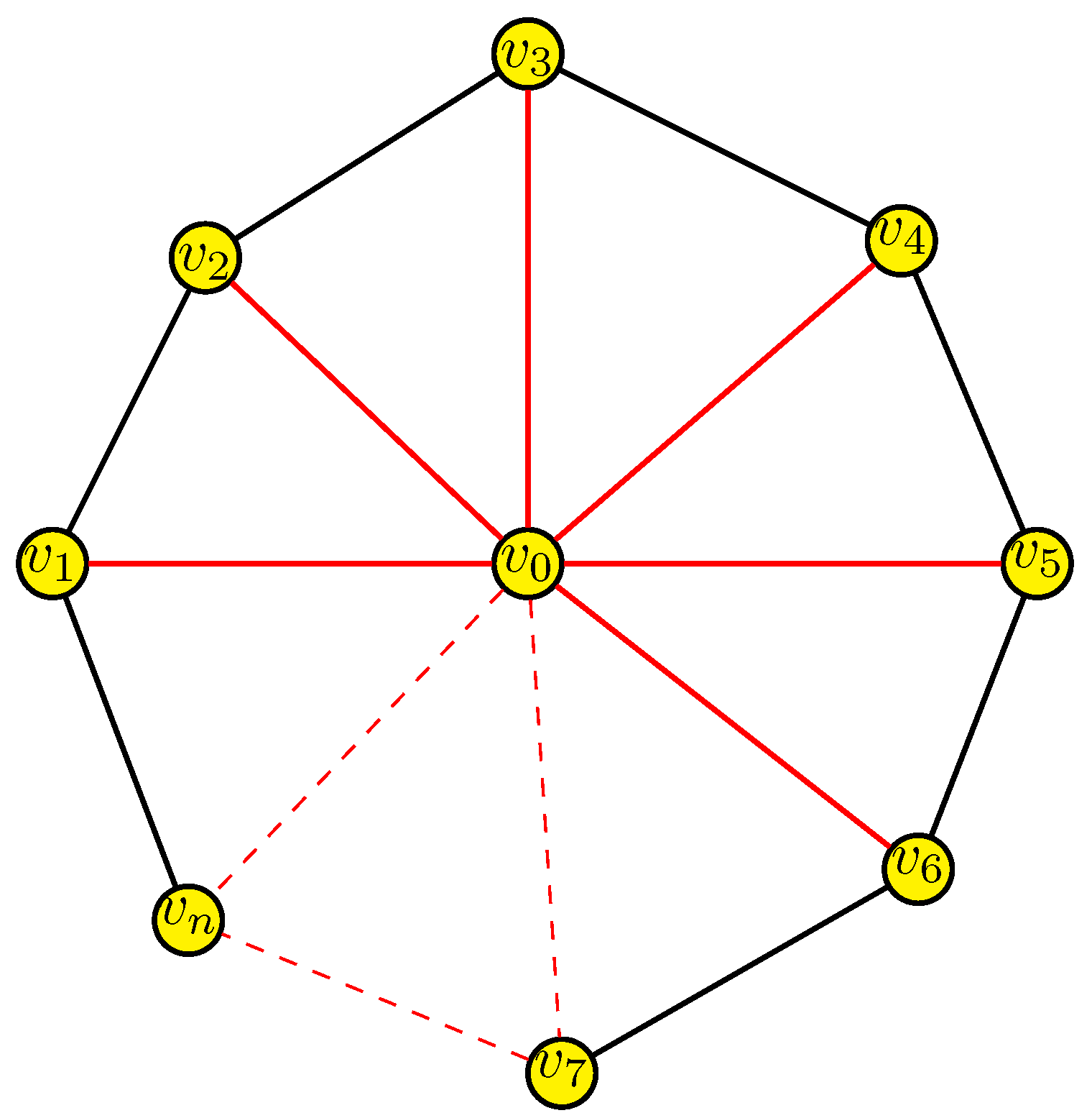
([13]). Let $\mathcal{L}$ be a non-void set and a binary relation $\perp \subseteq \mathcal{L}\times \mathcal{L}$ satisfying the condition:

$$\exists {\zeta }_0\in \mathcal{L}:(\forall \zeta \in \mathcal{L},\zeta \perp {\zeta }_0)or(\forall \zeta \in \mathcal{L},{\zeta }_0\perp \zeta ).$$

Then, $(\mathcal{L},\perp )$ is called an orthogonal set (O-set for short).

Example 1.

A wheel graph ${\mathcal{W}}_n$ is a graph with $n>3$, vertex $v_0$ connecting to all vertices, forming $(n-1)$-cycles; see Figure 1. Let $\mathcal{L}=\{{\mathcal{W}}_n:n>3\}$. Define ${\upsilon }_1\perp {\upsilon }_2$ if there is a connection from ${\upsilon }_1$ to ${\upsilon }_2$. Then, $(\mathcal{L},\perp )$ is an $\mathsf{O}$-set.

Definition 4

([13]). A sequence $\left\{{\zeta }_{\eta }\right\}$ defined on the O-set $(\mathcal{L},\perp )$ is called an orthogonal sequence (briefly, O-sequence) if

$$(\forall \eta \in \mathbb{N},{\zeta }_{\eta }\perp {\zeta }_{\eta +1})or(\forall \eta \in \mathbb{N},{\zeta }_{\eta +1}\perp {\zeta }_{\eta }).$$

Definition 5

([13]). Let $(\mathcal{L},\perp )$ be an O-set. Then, a self-map $\mathrm{H}$ on $\mathcal{L}$ is called ⊥-preserving if $\mathrm{H}\zeta \perp \mathrm{H}\xi$ whenever $\zeta \perp \xi$.

Aiman et al. [21] introduced the concepts of orthogonal Branciari metric spaces and its related properties.

Definition 6

([21]). The triplet $(\mathcal{L},\perp ,\pi )$ is said to be an orthogonal Branciari metric space (OBMS) if $(\mathcal{L},\perp )$ is an O-set and $(\mathcal{L},\pi )$ is a BMS.

Definition 7

([21]). Let $(\mathcal{L},\perp ,\pi )$ be an OBMS. Then, the self-map $\mathrm{H}$ on $\mathcal{L}$ is called orthogonal continuous (or ⊥-continuous) in $\zeta \in \mathcal{L}$ if for each O-sequence $\left\{{\zeta }_{\eta }\right\}$ in $\mathcal{L}$ with $\underset{\eta \to \infty }{lim}{\zeta }_{\eta }\to \zeta$, we obtain $\underset{\eta \to \infty }{lim}\mathrm{H}\left({\zeta }_{\eta }\right)\to \mathrm{H}\left(\zeta \right)$.

Furthermore, $\mathrm{H}$ is said to be ⊥-continuous on $\mathcal{L}$ if $\mathrm{H}$ is ⊥-continuous for every $\zeta \in \mathcal{L}$.

Definition 8

([21]). Let $(\mathcal{L},\perp ,\pi )$ be an OBMS; then, the O-sequence $\left\{{\zeta }_{\eta }\right\}\in \mathcal{L}$ converges to $\zeta \in \mathcal{L}$ if $\underset{\eta \to \infty }{lim}\pi ({\zeta }_{\eta },\zeta )\to 0$. Hence, we get ${\zeta }_{\eta }\to \zeta$.

Definition 9

([21]). Let $(\mathcal{L},\perp ,\pi )$ be an OBMS. We say that the O-sequence $\left\{{\zeta }_{\eta }\right\}\in \mathcal{L}$ is a Cauchy O-sequence if $\underset{\eta ,\omega \to \infty }{lim}\pi ({\zeta }_{\eta },{\zeta }_{\omega })\to 0$.

Definition 10

([21]). Let $(\mathcal{L},\perp ,\pi )$ be an OBMS. We say that the OBMS is orthogonal-complete (briefly, O-complete) if every Cauchy O-sequence is convergent.

Arul Joseph, Gunaseelan, Lee, and Park [19] introduced the orthogonal $\alpha$-admissible concepts as follows.

Definition 11

([19]). Let $\mathrm{H}$ be a self-map on $\mathcal{L}$ and a function $\alpha :\mathcal{L}\times \mathcal{L}\to [0,\infty )$. Then, $\mathrm{H}$ is said to be orthogonal α-admissible whenever $\zeta \perp \xi$ and $\alpha (\zeta ,\xi )\ge 1\Rightarrow \alpha (\mathrm{H}\zeta ,\mathrm{H}\xi )\ge 1$.

The following example shows that each $\alpha$-admissible is an orthogonal $\alpha$-admissible, but the converse is not true.

Example 2.

Let $\mathcal{L}=[0,1]$ with usual metric π and let $\mathrm{H}:\mathcal{L}\to \mathcal{L}$ be defined by

$$\mathrm{H}\left(\zeta \right)=\left\{\begin{array}{cc}\frac{\zeta }{2},\hfill & \mathit{if}\zeta \ne 1;\hfill \\ 1,\hfill & \mathit{otherwise}.\hfill \end{array}\right.$$

Now, define $\zeta \perp \xi$ if $\zeta \xi \le min\{\zeta ,\xi \}$. Note that $0\perp \zeta$ for all $\zeta \in \mathcal{L}$. Hence, $(\mathcal{L},\perp )$ is an O-set.

First, we shall show that $\mathrm{H}$ is orthogonal α-admissible. Indeed, if $\zeta \perp \xi$ and $\alpha (\zeta ,\xi )\ge 1$, then $\zeta \xi \le \zeta$ and $\zeta \xi \le \xi$. Suppose $\zeta \xi \ge 1$; this shows that $\zeta =1$ and $\xi =1$. Thus, $\alpha \left(\mathrm{H}\right(\zeta ),\mathrm{H}(\xi \left)\right)=\alpha (1,1)=1$. On the other hand, $\mathrm{H}$ is not α-admissible. Because $\alpha \left(\frac{3}{2},1\right)=\frac{3}{2}$ and $\alpha \left(\mathrm{H}\left(\frac{3}{2}\right),\mathrm{H}\left(1\right)\right)=\alpha \left(\frac{3}{4},1\right)=\frac{3}{4}$.

Definition 12

([19]). A self-map $\mathrm{H}$ on $\mathcal{L}$ is called an orthogonal triangular α-admissible if

(H1)

$\mathrm{H}$ is orthogonal α-admissible;

(H2)

whenever $\zeta \perp \mathfrak{p},\mathfrak{p}\perp \xi$, $\alpha (\zeta ,\mathfrak{p})\ge 1$ and $\alpha (\mathfrak{p},\xi )\ge 1$ implies that $\alpha (\zeta ,\xi )\ge 1$ for all $\zeta ,\mathfrak{p},\xi \in \mathcal{L}$.

Definition 13

([19]). Let $\mathrm{H}$ be a self-map on $\mathcal{L}$ and a function $\alpha :\mathcal{L}\times \mathcal{L}\to [0,\infty )$. We say that $\mathrm{H}$ is orthogonal α-orbital admissible

(H3)

whenever $\zeta \perp \mathrm{H}\zeta$ and $\alpha (\zeta ,\mathrm{H}\zeta )\ge 1$ implies that $\alpha (\mathrm{H}\zeta ,{\mathrm{H}}^2\zeta )\ge 1$.

Kirk and Shahzad [10] introduced the following lemma assertion that a Branciari metric space is a Hausdorff topological space with a neighborhood basis.

Lemma 1

([10]). Let $\left\{{\zeta }_{\eta }\right\}$ be a Cauchy sequence in $(\mathcal{L},\perp ,\pi )$ such that $\underset{\eta \to \infty }{lim}\pi ({\zeta }_{\eta },\zeta )\to 0$, for all $\zeta \in \mathcal{L}$. Then, $\underset{\eta \to \infty }{lim}\pi ({\zeta }_{\eta },\xi )\to \pi (\zeta ,\xi ),\forall \xi \in \mathcal{L}.$ In particular, $\left\{{\zeta }_{\eta }\right\}$ does not converge to ξ if $\xi \ne \zeta$.

Popescu [8] initialized the following lemma needed below.

Lemma 2

([8]). Let there exists a triangular α-orbital admissible self-map $\mathrm{H}$ on $\mathcal{L}$ and there exists ${\zeta }_1\in \mathcal{L}$ such that $\alpha ({\zeta }_1,\mathrm{H}{\zeta }_1)\ge 1$. Let $\left\{{\zeta }_{\eta }\right\}$ be a sequence defined as ${\zeta }_{\eta +1}=\mathrm{H}{\zeta }_{\eta }$. Then, $\alpha ({\zeta }_{\eta },{\zeta }_{\omega })\ge 1\forall \omega ,\eta \in \mathbb{N}$.

Very recently, Arshad et al. [12] established the following main results in the setting of the Branciari metric space with triangular $\alpha$-orbital admissible mapping. In this article, inspired by Muhammad’s work, we introduce an orthogonal triangular $\alpha$-orbital admissible mapping and an orthogonal triangular $\alpha$-orbital attractive mapping via orthogonal generalized contraction. We present an application of our orthogonal generalized contraction to the solution of integro-differential equations.

3. Main Results

First, we define an orthogonal triangular $\alpha$-orbital admissible mapping and with an example.

Definition 14.

Let $\mathrm{H}$ be a self-map on $\mathcal{L}$ and a function $\alpha :\mathcal{L}\times \mathcal{L}\to [0,\infty )$. We say that $\mathrm{H}$ is orthogonal triangular α-orbital admissible if it is satisfied $\left({\mathrm{H}}_3\right)$ and

(H4)

whenever $\zeta \perp \xi ,\xi \perp \mathrm{H}\xi ,\alpha (\zeta ,\xi )\ge 1$ and $\alpha (\xi ,\mathrm{H}\xi )\ge 1$ implies that $\alpha (\zeta ,\mathrm{H}\xi )\ge 1$.

Example 3.

Let $\mathcal{L}=\{0,1,2,3\},\pi :\mathcal{L}\times \mathcal{L}\to \mathbb{R}$ with the usual metric $\pi (\zeta ,\xi )=|\zeta -\xi |,\mathrm{H}:\mathcal{L}\to \mathcal{L}$ such that

$$\mathrm{H}\left(\zeta \right)=\left\{\begin{array}{cc}\zeta ,\hfill & \mathit{if}\zeta \in \{0,3\};\hfill \\ 1,\hfill & \mathit{if}\zeta \in \left\{2\right\};\hfill \\ 2,\hfill & \mathit{if}\zeta \in \left\{1\right\}.\hfill \end{array}\right.$$

Let $\alpha :\mathcal{L}\times \mathcal{L}\to [0,\infty )$ be defined by

$$\alpha (\zeta ,\xi )=\left\{\begin{array}{cc}1,\hfill & \mathit{if}(\zeta ,\xi )\in \left\{\right(0,1),(0,2),(1,1),(2,2),(1,2),(2,1),(1,3),(2,3\left)\right\};\hfill \\ 0,\hfill & \mathit{otherwise}.\hfill \end{array}\right.$$

Clearly, $\mathrm{H}$ is orthogonal triangular α-orbital admissible and $\mathrm{H}$ is orthogonal α-orbital admissible, but $\mathrm{H}$ is not orthogonal triangular α-admissible.

Arshad et al. [12] proved fixed-point results in Branrciari metric spaces via triangular $\alpha$-orbital admissible mappings. Inspired by [12], we prove fixed-point results via orthogonal triangular $\alpha$-orbital admissible map using a continuity hypothesis.

Theorem 1.

Let $\mathrm{H}$ be a self-map on orthogonal complete Branciari metric space $(\mathcal{L},\perp ,\pi )$ and $\alpha :\mathcal{L}\times \mathcal{L}\to [0,\infty )$ such that

(i) 

$\exists \vartheta \in ⊝$ and $\kappa \in (0,1)$ such that

$$\zeta ,\xi \in \mathcal{L}\mathit{with}\zeta \perp \xi [\pi (\mathrm{H}\zeta ,\mathrm{H}\xi )>0\Rightarrow \alpha (\zeta ,\xi )·\vartheta \left(\pi (\mathrm{H}\zeta ,\mathrm{H}\xi )\right)\le {\left[\vartheta \left(R(\zeta ,\xi )\right)\right]}^{\kappa }],$$

where

$$R(\zeta ,\xi )=max\left\{\pi (\zeta ,\xi ),\pi (\zeta ,\mathrm{H}\zeta ),\pi (\xi ,\mathrm{H}\xi ),\frac{\pi (\zeta ,\mathrm{H}\zeta )\pi (\xi ,\mathrm{H}\xi )}{1+\pi (\zeta ,\xi )}\right\};$$

(ii) 

$\exists {\zeta }_1\in \mathcal{L}$ such that $\alpha ({\zeta }_1,\mathrm{H}{\zeta }_1)\ge 1$ and $\alpha ({\zeta }_1,{\mathrm{H}}^2{\zeta }_1)\ge 1$;

(iii) 

$\mathrm{H}$ is an orthogonal triangular α-orbital admissible;

(iv) 

$\mathrm{H}$ is ⊥-preserving;

(v) 

$\mathrm{H}$ is ⊥-continuous.

Then $\mathrm{H}$ has a fixed point ${\zeta }_{*}\in \mathcal{L}$.

Proof. 

Since $(\mathcal{L},\perp )$ is an O-set,

$$\exists {\zeta }_0\in \mathcal{L}:(forall\zeta \in \mathcal{L},\zeta \perp {\zeta }_0)or(forall\zeta \in \mathcal{L},{\zeta }_0\perp \zeta ).$$

It follows that ${\zeta }_0\perp \mathrm{H}{\zeta }_{0}or\mathrm{H}{\zeta }_0\perp {\zeta }_0$.

By condition (ii), there exists ${\zeta }_1\in \mathcal{L}$ such that $\alpha ({\zeta }_1,\mathrm{H}{\zeta }_1)\ge 1$ and $\alpha ({\zeta }_1,{\mathrm{H}}^2{\zeta }_1)\ge 1$, which implies ${\zeta }_0\perp \mathrm{H}{\zeta }_0$ or $\mathrm{H}{\zeta }_0\perp {\zeta }_0$ and ${\zeta }_0\perp {\mathrm{H}}^2{\zeta }_{0}or{\mathrm{H}}^2{\zeta }_0\perp {\zeta }_0.$

Let ${\zeta }_1={\mathrm{H}}^2{\zeta }_0=\mathrm{H}{\zeta }_1,{\zeta }_2={\mathrm{H}}^2{\zeta }_1,{\zeta }_3=\mathrm{H}{\zeta }_2={\mathrm{H}}^3{\zeta }_1,\dots ,{\zeta }_{\eta }=\mathrm{H}{\zeta }_{\eta -1}={\mathrm{H}}^{\eta }{\zeta }_1$ for all $\eta \ge 1.$ Then $\left\{{\mathrm{H}}^{\eta }{\zeta }_1\right\}$ is an O-sequence in $\mathcal{L}$, since $\mathrm{H}$ is ⊥-preserving.

Condition (iii) implies that $\alpha ({\mathrm{H}}^{\eta }{\zeta }_1,{\mathrm{H}}^{\eta +1}{\zeta }_1)\ge 1$ for all $\eta \ge 1.$

If ${\mathrm{H}}^{{\eta }_0}{\zeta }_1={\mathrm{H}}^{{\eta }_0+1}{\zeta }_1$ for any ${\eta }_0\ge 1$, then ${\mathrm{H}}^{{\eta }_0}{\zeta }_1$ has a fixed point of $\mathrm{H}$. Assume that ${\mathrm{H}}^{\eta }{\zeta }_1\ne {\mathrm{H}}^{\eta +1}{\zeta }_1$ for all $\eta \ge 1$; we obtain $\alpha (\mathrm{H}{\zeta }_1,{\mathrm{H}}^2{\zeta }_1)\ge 1$, since $\mathrm{H}$ is an orthogonal $\alpha$-admissible mapping and $\alpha ({\zeta }_1,\mathrm{H}{\zeta }_1)\ge 1$. By continuing in this way,

$$\alpha ({\mathrm{H}}^{\eta }{\zeta }_1,{\mathrm{H}}^{\eta +1}{\zeta }_1)\ge 1,\forall \eta \ge 1.$$

(1)

Furthermore, since $\mathrm{H}$ is orthogonal $\alpha$-admissible mapping and $\alpha ({\zeta }_1,{\mathrm{H}}^2{\zeta }_1)\ge 1$, we deduce that $\alpha (\mathrm{H}{\zeta }_1,{\mathrm{H}}^3{\zeta }_1)\ge 1$. By continuing this process,

$$\alpha ({\mathrm{H}}^{\eta }{\zeta }_1,{\mathrm{H}}^{\eta +2}{\zeta }_1)\ge 1,\forall \eta \ge 1.$$

(2)

From condition (i) and (1), we write that for every $\eta \ge 1$,

$$\begin{array}{cc}\hfill \vartheta \left(\pi \left({\mathrm{H}}^{\eta }{\zeta }_1,{\mathrm{H}}^{\eta +1}{\zeta }_1\right)\right)& \le \alpha \left({\mathrm{H}}^{\eta -1}{\zeta }_1,{\mathrm{H}}^{\eta }{\zeta }_1\right)·\vartheta \left(\pi \left({\mathrm{H}}^{\eta -1}{\zeta }_1,{\mathrm{H}}^{\eta }{\zeta }_1\right)\right)\hfill \\ \hfill & \le \left[\vartheta \right(max\{\pi \left({\mathrm{H}}^{\eta -1}{\zeta }_1,{\mathrm{H}}^{\eta }{\zeta }_1\right),\pi \left({\mathrm{H}}^{\eta -1}{\zeta }_1,\mathrm{H}{\mathrm{H}}^{\eta -1}{\zeta }_1\right),\hfill \\ \hfill & \pi \left({\mathrm{H}}^{\eta }{\zeta }_1,\mathrm{H}{\mathrm{H}}^{\eta }{\zeta }_1\right),\frac{\pi \left({\mathrm{H}}^{\eta -1}{\zeta }_1,\mathrm{H}{\mathrm{H}}^{\eta -1}{\zeta }_1\right)·\pi \left({\mathrm{H}}^{\eta }{\zeta }_1,\mathrm{H}{\mathrm{H}}^{\eta }{\zeta }_1\right)}{1+\pi \left({\mathrm{H}}^{\eta -1}{\zeta }_1,{\mathrm{H}}^{\eta }{\zeta }_1\right)}\left\}\right){]}^{\kappa }\hfill \\ \hfill & =\left[\vartheta \right(max\{\pi \left({\mathrm{H}}^{\eta -1}{\zeta }_1,{\mathrm{H}}^{\eta }{\zeta }_1\right),\pi \left({\mathrm{H}}^{\eta }{\zeta }_1,{\mathrm{H}}^{\eta +1}{\zeta }_1\right),\hfill \\ \hfill & \frac{\pi \left({\mathrm{H}}^{\eta -1}{\zeta }_1,{\mathrm{H}}^{\eta }{\zeta }_1\right)·\pi \left({\mathrm{H}}^{\eta }{\zeta }_1,{\mathrm{H}}^{\eta +1}{\zeta }_1\right)}{1+\pi \left({\mathrm{H}}^{\eta -1}{\zeta }_1,{\mathrm{H}}^{\eta }{\zeta }_1\right)}\left\}\right){]}^{\kappa }\hfill \\ \hfill & ={\left[\vartheta \left(max\left\{\pi \left({\mathrm{H}}^{\eta -1}{\zeta }_1,{\mathrm{H}}^{\eta }{\zeta }_1\right),\pi \left({\mathrm{H}}^{\eta }{\zeta }_1,{\mathrm{H}}^{\eta +1}{\zeta }_1\right)\right\}\right)\right]}^{\kappa }.\hfill \end{array}$$

(3)

If $\exists \eta \ge 1$ such that

$$max\left\{\pi \left({\mathrm{H}}^{\eta -1}{\zeta }_1,{\mathrm{H}}^{\eta }{\zeta }_1\right),\pi \left({\mathrm{H}}^{\eta }{\zeta }_1,{\mathrm{H}}^{\eta +1}{\zeta }_1\right)\right\}=\pi \left({\mathrm{H}}^{\eta }{\zeta }_1,{\mathrm{H}}^{\eta +1}{\zeta }_1\right),$$

then inequality (3) turns into

$$\vartheta \left(\pi \left({\mathrm{H}}^{\eta }{\zeta }_1,{\mathrm{H}}^{\eta +1}{\zeta }_1\right)\right)\le {\left[\vartheta \left(\pi \left({\mathrm{H}}^{\eta }{\zeta }_1,{\mathrm{H}}^{\eta +1}{\zeta }_1\right)\right)\right]}^{\kappa }.$$

This implies

$$ln\left[\vartheta \left(\pi \left({\mathrm{H}}^{\eta }{\zeta }_1,{\mathrm{H}}^{\eta +1}{\zeta }_1\right)\right)\right]\le kln\left[\vartheta \left(\pi \left({\mathrm{H}}^{\eta }{\zeta }_1,{\mathrm{H}}^{\eta +1}{\zeta }_1\right)\right)\right].$$

This is a reductio absurdum with $\kappa \in (0,1)$. Then

$$max\{\pi ({\mathrm{H}}^{\eta -1}{\zeta }_1,{\mathrm{H}}^{\eta }{\zeta }_1),\pi ({\mathrm{H}}^{\eta }{\zeta }_1,{\mathrm{H}}^{\eta +1}{\zeta }_1)\}=\pi ({\mathrm{H}}^{\eta -1}{\zeta }_1,{\mathrm{H}}^{\eta }{\zeta }_1),\forall \eta \ge 1.$$

Thus, from (3), we have

$$\vartheta \left(\pi \left({\mathrm{H}}^{\eta }{\zeta }_1,{\mathrm{H}}^{\eta +1}{\zeta }_1\right)\right)\le {\left[\vartheta \left(\pi \left({\mathrm{H}}^{\eta -1}{\zeta }_1,{\mathrm{H}}^{\eta }{\zeta }_1\right)\right)\right]}^{\kappa },\forall \eta \ge 1.$$

This implies

$$\begin{array}{cc}\hfill \vartheta \left(\pi ({\mathrm{H}}^{\eta }{\zeta }_1,{\mathrm{H}}^{\eta +1}{\zeta }_1)\right)& \le {\left[\vartheta \left(\pi ({\mathrm{H}}^{\eta -1}{\zeta }_1,{\mathrm{H}}^{\eta }{\zeta }_1)\right)\right]}^{\kappa }\hfill \\ \hfill & \le {\left[\vartheta \left(\pi \left({\mathrm{H}}^{\eta -2}{\zeta }_1,{\mathrm{H}}^{\eta -1}{\zeta }_1\right)\right)\right]}^{{\kappa }^2}\hfill \\ \hfill & \le {\left[\vartheta \left(\pi \left({\mathrm{H}}^{\eta -3}{\zeta }_1,{\mathrm{H}}^{\eta -2}{\zeta }_1\right)\right)\right]}^{{\kappa }^3}\hfill \\ \hfill & ⋮\hfill \\ \hfill & \le {\left[\vartheta \left(\pi \left({\zeta }_1,\mathrm{H}{\zeta }_1\right)\right)\right]}^{{\kappa }^{\eta }}.\hfill \end{array}$$

Thus, we have

$$1\le \vartheta \left(\pi \left({\mathrm{H}}^{\eta }{\zeta }_1,{\mathrm{H}}^{\eta +1}{\zeta }_1\right)\right)\le {\left[\vartheta \left(\pi \left({\zeta }_1,\mathrm{H}{\zeta }_1\right)\right)\right]}^{{\kappa }^{\eta }},\forall \eta \ge 1.$$

(4)

Letting $\eta \to \infty$, we obtain

$$\begin{array}{c}\hfill \underset{\eta \to \infty }{lim}\vartheta \left(\pi \left({\mathrm{H}}^{\eta }{\zeta }_1,{\mathrm{H}}^{\eta +1}{\zeta }_1\right)\right)=1,\end{array}$$

(5)

which together with $\left({⊝}_2\right)$ gives $\underset{\eta \to \infty }{lim}\pi \left({\mathrm{H}}^{\eta }{\zeta }_1,{\mathrm{H}}^{\eta +1}{\zeta }_1\right)=0.$

From ${⊝}_3$, there exists $\mathfrak{r}\in (0,1)$ and $\ell \in (0,\infty ]$ such that

$$\underset{\eta \to \infty }{lim}\frac{\vartheta \left(\pi \left({\mathrm{H}}^{\eta }{\zeta }_1,{\mathrm{H}}^{\eta +1}{\zeta }_1\right)\right)-1}{\pi {\left({\mathrm{H}}^{\eta }{\zeta }_1,{\mathrm{H}}^{\eta +1}{\zeta }_1\right)}^{\mathfrak{r}}}=\ell .$$

In this case, assume that $\ell <\infty$ and let $\mathfrak{B}=\frac{l}{2}>0$.

From the definition of limit, $\exists {\eta }_0\ge 1$, such that

$$\left|\frac{\vartheta \left(\pi \left({\mathrm{H}}^{\eta }{\zeta }_1,{\mathrm{H}}^{\eta +1}{\zeta }_1\right)\right)-1}{\pi {\left({\mathrm{H}}^{\eta }{\zeta }_1,{\mathrm{H}}^{\eta +1}{\zeta }_1\right)}^{\mathfrak{r}}}-\ell \right|\le \mathfrak{B},\forall \eta \ge {\eta }_0.$$

This implies

$$\frac{\vartheta \left(\pi \left({\mathrm{H}}^{\eta }{\zeta }_1,{\mathrm{H}}^{\eta +1}{\zeta }_1\right)\right)-1}{\pi {\left({\mathrm{H}}^{\eta }{\zeta }_1,{\mathrm{H}}^{\eta +1}{\zeta }_1\right)}^{\mathfrak{r}}}\ge \ell -\mathfrak{B}=\mathfrak{B},\forall \eta \ge {\eta }_0.$$

Then

$$\eta {\left[\pi \left({\mathrm{H}}^{\eta }{\zeta }_1,{\mathrm{H}}^{\eta +1}{\zeta }_1\right)\right]}^{\mathfrak{r}}\le \mathfrak{A}\eta \left[\vartheta \left(\pi \left({\mathrm{H}}^{\eta }{\zeta }_1,{\mathrm{H}}^{\eta +1}{\zeta }_1\right)\right)-1\right],\forall \eta \ge {\eta }_0,$$

where $\mathfrak{A}=\frac{1}{\mathfrak{B}}$. Now, let $\ell =\infty$ and let $\mathfrak{B}>0$.

From the limit definition, there exists ${\eta }_0\ge 1$ such that

$$\frac{\vartheta \left(\pi \left({\mathrm{H}}^{\eta }{\zeta }_1,{\mathrm{H}}^{\eta +1}{\zeta }_1\right)\right)-1}{\pi {\left({\mathrm{H}}^{\eta }{\zeta }_1,{\mathrm{H}}^{\eta +1}{\zeta }_1\right)}^{\mathfrak{r}}}\ge \mathfrak{B},\forall \eta \ge {\eta }_0.$$

This implies

$$\eta {\left[\pi \left({\mathrm{H}}^{\eta }{\zeta }_1,{\mathrm{H}}^{\eta +1}{\zeta }_1\right)\right]}^{\mathfrak{r}}\le \mathfrak{A}\eta \left[\vartheta \left(\pi \left({\mathrm{H}}^{\eta }{\zeta }_1,{\mathrm{H}}^{\eta +1}{\zeta }_1\right)\right)-1\right],\forall \eta \ge {\eta }_0,$$

where $\mathfrak{A}=\frac{1}{\mathfrak{B}}$.

Then $\exists \mathfrak{A}>0$ and ${\eta }_0\ge 1$ such that

$$\eta {\left[\pi \left({\mathrm{H}}^{\eta }{\zeta }_1,{\mathrm{H}}^{\eta +1}{\zeta }_1\right)\right]}^{\mathfrak{r}}\le \mathfrak{A}\eta \left[\vartheta \left(\pi \left({\mathrm{H}}^{\eta }{\zeta }_1,{\mathrm{H}}^{\eta +1}{\zeta }_1\right)\right)-1\right],\forall \eta \ge {\eta }_0.$$

By using (4), we obtain

$$\eta {\left[\pi \left({\mathrm{H}}^{\eta }{\zeta }_1,{\mathrm{H}}^{\eta +1}{\zeta }_1\right)\right]}^{\mathfrak{r}}\le \mathfrak{A}\eta {\left(\left[\vartheta \left(\pi ({\zeta }_1,\mathrm{H}{\zeta }_1\right)\right)\right]}^{{\kappa }^{\eta }}-1),\forall \eta \ge {\eta }_0.$$

(6)

Taking $\eta \to \infty$ in Equation (6), we have

$$\underset{\eta \to \infty }{lim}\eta {\left[\pi \left({\mathrm{H}}^{\eta }{\zeta }_1,{\mathrm{H}}^{\eta +1}{\zeta }_1\right)\right]}^{\mathfrak{r}}=0.$$

Thus, $\exists {\eta }_1\in \mathbb{N}$ such that

$$\pi \left({\mathrm{H}}^{\eta }{\zeta }_1,{\mathrm{H}}^{\eta +1}{\zeta }_1\right)\le \frac{1}{{\eta }^{\frac{1}{\mathfrak{r}}}},\forall \eta \ge {\eta }_1.$$

(7)

Now, we show that ${\zeta }_{*}$ is a periodic point in $\mathrm{H}$.

Conversely, we assume that ${\mathrm{H}}^{\eta }{\zeta }_1\ne {\mathrm{H}}^{\omega }{\zeta }_1,\forall \eta ,\omega \ge 1$, such that $\eta \ne \omega$.

By (i) and Equation (2), we obtain

$$\begin{array}{cc}\hfill \vartheta \left(\pi \left({\mathrm{H}}^{\eta }{\zeta }_1,{\mathrm{H}}^{\eta +2}{\zeta }_1\right)\right)& \le \alpha \left({\mathrm{H}}^{\eta -1}{\zeta }_1,{\mathrm{H}}^{\eta +1}{\zeta }_1\right)·\vartheta \left(\pi \left({\mathrm{H}}^{\eta -1}{\zeta }_1,{\mathrm{H}}^{\eta +1}{\zeta }_1\right)\right)\hfill \\ \hfill & \le \left[\vartheta \right(max\{\pi \left({\mathrm{H}}^{\eta -1}{\zeta }_1,{\mathrm{H}}^{\eta +1}{\zeta }_1\right),\pi \left({\mathrm{H}}^{\eta -1}{\zeta }_1,\mathrm{H}{\mathrm{H}}^{\eta -1}{\zeta }_1\right),\hfill \\ \hfill & \pi \left({\mathrm{H}}^{\eta +1}{\zeta }_1,\mathrm{H}{\mathrm{H}}^{\eta +1}{\zeta }_1\right),\frac{\pi \left({\mathrm{H}}^{\eta -1}{\zeta }_1,\mathrm{H}{\mathrm{H}}^{\eta -1}{\zeta }_1\right)·\pi \left({\mathrm{H}}^{\eta +1}{\zeta }_1,\mathrm{H}{\mathrm{H}}^{\eta +1}{\zeta }_1\right)}{1+\pi \left({\mathrm{H}}^{\eta -1}{\zeta }_1,{\mathrm{H}}^{\eta +1}{\zeta }_1\right)}\left\}\right){]}^{\kappa }\hfill \\ \hfill & =\left[\vartheta \right(max\{\pi \left({\mathrm{H}}^{\eta -1}{\zeta }_1,{\mathrm{H}}^{\eta +1}{\zeta }_1\right),\pi \left({\mathrm{H}}^{\eta -1}{\zeta }_1,{\mathrm{H}}^{\eta }{\zeta }_1\right),\hfill \\ \hfill & \pi \left({\mathrm{H}}^{\eta +1}{\zeta }_1,{\mathrm{H}}^{\eta +2}{\zeta }_1\right),\frac{\pi \left({\mathrm{H}}^{\eta -1}{\zeta }_1,{\mathrm{H}}^{\eta }{\zeta }_1\right)·\pi \left({\mathrm{H}}^{\eta +1}{\zeta }_1,{\mathrm{H}}^{\eta +2}{\zeta }_1\right)}{1+\pi \left({\mathrm{H}}^{\eta -1}{\zeta }_1,{\mathrm{H}}^{\eta +1}{\zeta }_1\right)}\left\}\right){]}^{\kappa }\hfill \\ \hfill & ={\left[\vartheta \left(max\left\{\pi \left({\mathrm{H}}^{\eta -1}{\zeta }_1,{\mathrm{H}}^{\eta +1}{\zeta }_1\right),\pi \left({\mathrm{H}}^{\eta -1}{\zeta }_1,{\mathrm{H}}^{\eta }{\zeta }_1\right),\pi \left({\mathrm{H}}^{\eta +1}{\zeta }_1,{\mathrm{H}}^{\eta +2}{\zeta }_1\right)\right\}\right)\right]}^{\kappa }.\hfill \end{array}$$

(8)

Since $\vartheta$ is non-decreasing and from (8), we obtain

$$\begin{array}{cc}\hfill \vartheta \left(\pi \left({\mathrm{H}}^{\eta }{\zeta }_1,{\mathrm{H}}^{\eta +2}{\zeta }_1\right)\right)& \le \left[max\left\{\vartheta \left(\pi \left({\mathrm{H}}^{\eta -1}{\zeta }_1,{\mathrm{H}}^{\eta +1}{\zeta }_1\right)\right),\vartheta \left(\pi \left({\mathrm{H}}^{\eta -1}{\zeta }_1,{\mathrm{H}}^{\eta }{\zeta }_1\right)\right)\right.\right.,\hfill \\ \hfill & {\left.\left.\vartheta \left(\pi \left({\mathrm{H}}^{\eta +1}{\zeta }_1,{\mathrm{H}}^{\eta +2}{\zeta }_1\right)\right)\right\}\right]}^{\kappa }.\hfill \end{array}$$

(9)

Let $\mathrm{I}={\left\{\eta \right\}}_{\eta \in \mathbb{N}}$, satisfying

$$\begin{array}{cc}\hfill {\mathfrak{p}}_{\eta }& =max\left\{\vartheta \left(\pi \left({\mathrm{H}}^{\eta -1}{\zeta }_1,{\mathrm{H}}^{\eta +1}{\zeta }_1\right)\right),\vartheta \left(\pi \left({\mathrm{H}}^{\eta -1}{\zeta }_1,{\mathrm{H}}^{\eta }{\zeta }_1\right)\right),\vartheta \left(\pi \left({\mathrm{H}}^{\eta +1}{\zeta }_1,{\mathrm{H}}^{\eta +2}{\zeta }_1\right)\right)\right\}\hfill \\ \hfill & =\vartheta \left(\pi \left({\mathrm{H}}^{\eta -1}{\zeta }_1,{\mathrm{H}}^{\eta +1}{\zeta }_1\right)\right).\hfill \end{array}$$

If $\left|\mathrm{I}\right|<\infty$, then $\exists \eta \ge 1$, such that ∀$\eta \ge N$,

$$\begin{array}{cc}\hfill & max\left\{\vartheta \left(\pi \left({\mathrm{H}}^{\eta -1}{\zeta }_1,{\mathrm{H}}^{\eta +1}{\zeta }_1\right)\right),\vartheta \left(\pi \left({\mathrm{H}}^{\eta -1}{\zeta }_1,{\mathrm{H}}^{\eta }{\zeta }_1\right)\right),\vartheta \left(\pi \left({\mathrm{H}}^{\eta +1}{\zeta }_1,{\mathrm{H}}^{\eta +2}{\zeta }_1\right)\right)\right\}\hfill \\ \hfill & =max\left\{\vartheta \left(\pi \left({\mathrm{H}}^{\eta -1}{\zeta }_1,{\mathrm{H}}^{\eta }{\zeta }_1\right)\right),\vartheta \left(\pi \left({\mathrm{H}}^{\eta +1}{\zeta }_1,{\mathrm{H}}^{\eta +2}{\zeta }_1\right)\right)\right\}.\hfill \end{array}$$

In this case, from (9), we obtain

$$1\le \vartheta \left(\pi \left({\mathrm{H}}^{\eta }{\zeta }_1,{\mathrm{H}}^{\eta +2}{\zeta }_1\right)\right)\le {\left[max\left\{\vartheta \left(\pi \left({\mathrm{H}}^{\eta -1}{\zeta }_1,{\mathrm{H}}^{\eta }{\zeta }_1\right)\right),\vartheta \left(\pi \left({\mathrm{H}}^{\eta +1}{\zeta }_1,{\mathrm{H}}^{\eta +2}{\zeta }_1\right)\right)\right\}\right]}^{\kappa },\forall \eta \ge N.$$

If, in the above inequality, taking $\eta \to \infty$ and using (5), we obtain

$$\underset{\eta \to \infty }{lim}\vartheta \left(\pi \left({\mathrm{H}}^{\eta }{\zeta }_1,{\mathrm{H}}^{\eta +2}{\zeta }_1\right)\right)=1.$$

Find a subsequence of $\left\{{\mathfrak{p}}_{\eta }\right\}$. If $\left|\mathrm{I}\right|=\infty$, then

$${\mathfrak{p}}_{\eta }=\vartheta \left(\pi \left({\mathrm{H}}^{\eta -1}{\zeta }_1,{\mathrm{H}}^{\eta +1}{\zeta }_1\right)\right).$$

In this case, from (9), we obtain

$$\begin{array}{cc}\hfill 1& \le \vartheta \left(\pi \left({\mathrm{H}}^{\eta }{\zeta }_1,{\mathrm{H}}^{\eta +2}{\zeta }_1\right)\right)\hfill \\ \hfill & \le {\left[\vartheta \left(\pi \left({\mathrm{H}}^{\eta -1}{\zeta }_1,{\mathrm{H}}^{\eta +1}{\zeta }_1\right)\right)\right]}^{\kappa }\hfill \\ \hfill & \le {\left[\vartheta \left(\pi \left({\mathrm{H}}^{\eta -2}{\zeta }_1,{\mathrm{H}}^{\eta }{\zeta }_1\right)\right)\right]}^{{\kappa }^2}\hfill \\ \hfill & ⋮\hfill \\ \hfill & \le {\left[\vartheta \left(\pi \left({\zeta }_1,{\mathrm{H}}^2{\zeta }_1\right)\right)\right]}^{{\kappa }^{\eta }},\hfill \end{array}$$

for large $\eta .$

Setting $\eta \to \infty$ in the above inequality, we obtain

$$\underset{\eta \to \infty }{lim}\vartheta \left(\pi \left({\mathrm{H}}^{\eta }{\zeta }_1,{\mathrm{H}}^{\eta +2}{\zeta }_1\right)\right)=1.$$

(10)

In all cases, (10) holds. Then, using (10) and $\left({⊝}_2\right)$, we have

$$\underset{\eta \to \infty }{lim}\pi \left({\mathrm{H}}^{\eta }{\zeta }_1,{\mathrm{H}}^{\eta +2}{\zeta }_1\right)=0.$$

Similarly, from $\left({⊝}_3\right)$, there exists ${\eta }_2\ge 1$ such that

$$\pi \left({\mathrm{H}}^{\eta }{\zeta }_1,{\mathrm{H}}^{\eta +2}{\zeta }_1\right)\le \frac{1}{{\eta }^{\frac{1}{\mathfrak{r}}}},\forall \eta \ge {\eta }_2.$$

(11)

Let $\mathfrak{h}=max\{{\eta }_0,{\eta }_1\}$. Now we raise the following cases.

Case 1: If $\omega >2$ is odd, then $\omega =2\mathfrak{L}+1$ for some $\mathfrak{L}\ge 1$; by Equation (7) $\forall \eta \ge \mathfrak{h}$, we obtain

$$\begin{array}{cc}\hfill \pi \left({\mathrm{H}}^{\eta }{\zeta }_1,{\mathrm{H}}^{\eta +\omega }{\zeta }_1\right)& \le \pi \left({\mathrm{H}}^{\eta }{\zeta }_1,{\mathrm{H}}^{\eta +1}{\zeta }_1\right)+\pi \left({\mathrm{H}}^{\eta +1}{\zeta }_1,{\mathrm{H}}^{\eta +2}{\zeta }_1\right)+\cdots +\pi \left({\mathrm{H}}^{\eta +2\mathfrak{L}}{\zeta }_1,{\mathrm{H}}^{\eta +2\mathfrak{L}+1}{\zeta }_1\right)\hfill \\ \hfill & \le \frac{1}{{\eta }^{\frac{1}{\mathfrak{r}}}}+\frac{1}{{(\eta +1)}^{\frac{1}{\mathfrak{r}}}}+\cdots +\frac{1}{{(\eta +2\mathfrak{L})}^{\frac{1}{\mathfrak{r}}}}\hfill \\ \hfill & \le \sum _{n=\eta }^{\infty }\frac{1}{n^{\frac{1}{\mathfrak{r}}}}.\hfill \end{array}$$

Case 2: If $\omega >2$ is even, then $\omega =2\mathfrak{L}$ for some $\mathfrak{L}\ge 2$; by Equations (7) and (11) $\forall \eta \ge \mathfrak{h}$, we obtain

$$\begin{array}{cc}\hfill \pi \left({\mathrm{H}}^{\eta }{\zeta }_1,{\mathrm{H}}^{\eta +\omega }{\zeta }_1\right)& \le \pi \left({\mathrm{H}}^{\eta }{\zeta }_1,{\mathrm{H}}^{\eta +2}{\zeta }_1\right)+\pi \left({\mathrm{H}}^{\eta +2}{\zeta }_1,{\mathrm{H}}^{\eta +3}{\zeta }_1\right)+\cdots +\pi \left({\mathrm{H}}^{\eta +2\mathfrak{L}-1}{\zeta }_1,{\mathrm{H}}^{\eta +2\mathfrak{L}}{\zeta }_1\right)\hfill \\ \hfill & \le \frac{1}{{\eta }^{\frac{1}{\mathfrak{r}}}}+\frac{1}{{(\eta +2)}^{\frac{1}{\mathfrak{r}}}}+\cdots +\frac{1}{{(\eta +2\mathfrak{L}-1)}^{\frac{1}{\mathfrak{r}}}}\hfill \\ \hfill & \le \sum _{i=\eta }^{\infty }\frac{1}{i^{\frac{1}{\mathfrak{r}}}}.\hfill \end{array}$$

Combining all cases, we thus have

$$\pi \left({\mathrm{H}}^{\eta }{\zeta }_1,{\mathrm{H}}^{\eta +\omega }{\zeta }_1\right)\le \sum _{n=\eta }^{\infty }\frac{1}{n^{\frac{1}{\mathfrak{r}}}},\forall \eta \ge \mathfrak{h},\omega \ge 1.$$

We conclude that $\left\{{\mathrm{H}}^{\eta }{\zeta }_1\right\}$ is a Cauchy O-sequence, since the series ${\sum }_{n=\eta }^{\infty }\frac{1}{n^{\frac{1}{\mathfrak{r}}}}$ converges, since $\frac{1}{\mathfrak{r}}>1$.

From O-completeness of $\mathcal{L}$, there is ${\zeta }_{*}\in \mathcal{L}$ such that ${\mathrm{H}}^{\eta }{\zeta }_1\to {\zeta }_{*}$ as $\eta \to \infty$. Since $\mathrm{H}$ is orthogonal continuous, we have

$${\zeta }_{*}=\underset{\eta \to \infty }{lim}{\mathrm{H}}^{\eta +1}{\zeta }_1=\underset{\eta \to \infty }{lim}\mathrm{H}\left({\mathrm{H}}^{\eta }{\zeta }_1\right)=\mathrm{H}\left(\underset{\eta \to \infty }{lim}{\mathrm{H}}^{\eta }{\zeta }_1\right)=\mathrm{H}{\zeta }_{*}.$$

We obtain ${\zeta }_{*}=\mathrm{H}{\zeta }_{*}$, a contradiction by our assumptions. Therefore, $\mathrm{H}$ has a periodic point.

Suppose fix$\left(\mathrm{H}\right)=\varphi$. Then $s>1$ and $\pi ({\zeta }_{*},\mathrm{H}{\zeta }_{*})>0$. Now,

$$\begin{array}{cc}\hfill \vartheta \left(\pi \left({\zeta }_{*},\mathrm{H}{\zeta }_{*}\right)\right)& =\vartheta \left(\pi \left({\mathrm{H}}^s{\zeta }_{*},{\mathrm{H}}^{s+1}{\zeta }_{*}\right)\right)\hfill \\ \hfill & \le \alpha \left({\mathrm{H}}^{s-1}{\zeta }_{*},{\mathrm{H}}^s{\zeta }_{*}\right)·\vartheta \left(\pi \left({\mathrm{H}}^s{\zeta }_{*},{\mathrm{H}}^{s+1}{\zeta }_{*}\right)\right)\hfill \\ \hfill & \le {\left[\vartheta \left(\pi \left({\zeta }_{*},\mathrm{H}{\zeta }_{*}\right)\right)\right]}^{{\kappa }^s}\hfill \\ \hfill & <\vartheta \left(\pi \left({\zeta }_{*},\mathrm{H}{\zeta }_{*}\right)\right),\hfill \end{array}$$

which is a contradiction with $k\in (0,1)$. Therefore, we have a non-empty set of fixed points of $\mathrm{H}$; that is, $\mathrm{H}$ has at least one fixed point. □

Arshad et al. [12] proved fixed-point results in Branrciari metric spaces via triangular $\alpha$-orbital admissible mappings. Inspired by [12], we prove the fixed point theorem on an orthogonal triangular $\alpha$-orbital admissible mapping using without a continuity hypothesis.

Theorem 2.

Let $\mathrm{H}$ be a self-map on orthogonal complete Branciari metric space $(\mathcal{L},\perp ,\pi )$ and a map $\alpha :\mathcal{L}\times \mathcal{L}\to [0,\infty )$ such that

(i) 

We can find $\vartheta \in ⊝$ and $\kappa \in (0,1)$ satisfying

$$\begin{array}{cc}\hfill \zeta ,\xi \in \mathcal{L}\mathit{with}\zeta \perp \xi & \left[\pi \right(\mathrm{H}\zeta ,\mathrm{H}\xi )>0,\pi (\mathrm{H}\zeta ,\mathrm{H}\xi )\ne 0\hfill \\ \hfill & \Rightarrow \alpha (\zeta ,\xi ).\vartheta \left(\pi (\mathrm{H}\zeta ,\mathrm{H}\xi )\right)\le {\left[\vartheta \left(R(\zeta ,\xi )\right)\right]}^{\kappa }],\hfill \end{array}$$

where

$$R(\zeta ,\xi )=max\left\{\pi (\zeta ,\xi ),\pi (\zeta ,\mathrm{H}\zeta ),\pi (\xi ,\mathrm{H}\xi ),\frac{\pi (\zeta ,\mathrm{H}\zeta )\pi (\xi ,\mathrm{H}\xi )}{1+\pi (\zeta ,\xi )}\right\};$$

(ii) 

$\exists {\zeta }_1\in \mathcal{L}$ such that $\alpha ({\zeta }_1,\mathrm{H}{\zeta }_1)\ge 1$ and $\alpha \left({\zeta }_1,{\mathrm{H}}^2{\zeta }_1\right)\ge 1$;

(iii) 

$\mathrm{H}$ is an orthogonal triangular α-orbital admissible mapping;

(iv) 

if $\left\{{\mathrm{H}}^{\eta }{\zeta }_1\right\}$ is an O-sequence in $\mathcal{L}$ such that $\alpha \left({\mathrm{H}}^{\eta }{\zeta }_1,{\mathrm{H}}^{\eta +1}{\zeta }_1\right)\ge 1$ for all η and ${\zeta }_{\eta }\to \zeta \in \mathcal{L}$ as $n\to \infty$; then, there exists a sub-sequence $\left\{{\mathrm{H}}^{\eta \left(\kappa \right)}{\zeta }_1\right\}$ of $\left\{{\mathrm{H}}^{\eta }{\zeta }_1\right\}$ such that $\alpha \left({\mathrm{H}}^{\eta \left(\kappa \right)}{\zeta }_1,\zeta \right)\ge 1,\forall \kappa$;

(v) 

ϑ is ⊥-continuous.

Then, $\mathrm{H}$ has a fixed point ${\zeta }_{*}\in \mathcal{L}$.

Proof. 

Since $(\mathcal{L},\perp )$ is an O-set,

$$\exists {\zeta }_0\in \mathcal{L}:(\forall \zeta \in \mathcal{L},\zeta \perp {\zeta }_0)or(\forall \zeta \in \mathcal{L},{\zeta }_0\perp \zeta ).$$

It follows that ${\zeta }_0\perp \mathrm{H}{\zeta }_{0}or\mathrm{H}{\zeta }_0\perp {\zeta }_0$.

Since there exists ${\zeta }_1\in \mathcal{L}$ such that $\alpha \left({\zeta }_1,\mathrm{H}{\zeta }_1\right)\ge 1$ and $\alpha \left({\zeta }_1,{\mathrm{H}}^2{\zeta }_1\right)\ge 1$,

$${\zeta }_0\perp \mathrm{H}{\zeta }_0\mathrm{or}\mathrm{H}{\zeta }_0\perp {\zeta }_0\mathrm{and}{\zeta }_0\perp {\mathrm{H}}^2{\zeta }_0\mathrm{or}{\mathrm{H}}^2{\zeta }_0\perp {\zeta }_0.$$

Let ${\zeta }_1={\mathrm{H}}^2{\zeta }_0=\mathrm{H}{\zeta }_1,{\zeta }_2={\mathrm{H}}^2{\zeta }_1,{\zeta }_3=\mathrm{H}{\zeta }_2={\mathrm{H}}^3{\zeta }_1,\dots ,{\zeta }_{\eta }=\mathrm{H}{\zeta }_{\eta -1}={\mathrm{H}}^{\eta }{\zeta }_1,\forall \eta \ge 1.$

If ${\mathrm{H}}^{{\eta }_0}{\zeta }_1={\mathrm{H}}^{{\eta }_0+1}{\zeta }_1$ for any ${\eta }_0\ge 1$, then it is clear that ${\mathrm{H}}^{{\eta }_0}{\zeta }_1$ has a fixed point of $\mathrm{H}$.

From condition (iv), which implies a sub-sequence $\left\{\left({\mathrm{H}}^{\eta \left(\kappa \right)}{\zeta }_1\right)\right\}$ of $\left\{\left({\mathrm{H}}^{\eta }{\zeta }_1\right)\right\}$ such that $\alpha \left({\mathrm{H}}^{\eta \left(\kappa \right)}{\zeta }_1,{\zeta }_{*}\right)\ge 1,\forall \kappa$.

Suppose that ${\mathrm{H}}^{\eta \left(\kappa \right)+1}{\zeta }_1\ne \mathrm{H}{\zeta }_{*}$; then, from condition (i), we have

$$\begin{array}{cc}\hfill \vartheta \left(\pi ({\mathrm{H}}^{\eta \left(\kappa \right)+1}{\zeta }_1,\mathrm{H}{\zeta }_{*})\right)& =\vartheta \left(\pi \left(\mathrm{H}\left({\mathrm{H}}^{\eta \left(\kappa \right)}{\zeta }_1\right),\mathrm{H}{\zeta }_{*}\right)\right)\hfill \\ \hfill & \le \alpha \left({\mathrm{H}}^{\eta \left(\kappa \right)}{\zeta }_1,{\zeta }_{*}\right)·\vartheta \left(\pi \left(\mathrm{H}\left({\mathrm{H}}^{\eta \left(\kappa \right)}{\zeta }_1\right),\mathrm{H}{\zeta }_{*}\right)\right)\hfill \\ \hfill & \le \left[\vartheta \right(max\{\pi \left({\mathrm{H}}^{\eta \left(\kappa \right)}{\zeta }_1,{\zeta }_{*}\right),\pi \left({\mathrm{H}}^{\eta \left(\kappa \right)}{\zeta }_1,\mathrm{H}{\mathrm{H}}^{\eta \left(\kappa \right)}{\zeta }_1\right),\pi \left({\zeta }_{*},\mathrm{H}{\zeta }_{*}\right),\hfill \\ \hfill & \frac{\pi \left({\mathrm{H}}^{\eta \left(\kappa \right)}{\zeta }_1,\mathrm{H}\left({\mathrm{H}}^{\eta \left(\kappa \right)}{\zeta }_1\right)\right)·\pi \left({\zeta }_{*},\mathrm{H}{\zeta }_{*}\right)}{1+\pi \left({\mathrm{H}}^{\eta \left(\kappa \right)}{\zeta }_1,{\zeta }_{*}\right)}\left\}\right){]}^{\kappa }\hfill \\ \hfill & =\left[\vartheta \right(max\{\pi \left({\mathrm{H}}^{\eta \left(\kappa \right)}{\zeta }_1,{\zeta }_{*}\right),\pi \left({\mathrm{H}}^{\eta \left(\kappa \right)}{\zeta }_1,{\mathrm{H}}^{\eta \left(\kappa \right)+1}{\zeta }_1\right),\pi \left({\zeta }_{*},\mathrm{H}{\zeta }_{*}\right),\hfill \\ \hfill & \frac{\pi \left({\mathrm{H}}^{\eta \left(\kappa \right)}{\zeta }_1,{\mathrm{H}}^{\eta \left(\kappa \right)+1}{\zeta }_1\right)·\pi \left({\zeta }_{*},\mathrm{H}{\zeta }_{*}\right)}{1+\pi \left({\mathrm{H}}^{\eta \left(\kappa \right)}{\zeta }_1,{\zeta }_{*}\right)}\left\}\right){]}^{\kappa }.\hfill \end{array}$$

(12)

Suppose that $\pi ({\zeta }_{*},\mathrm{H}{\zeta }_{*})>0$. Now, taking the limit as $\kappa \to \infty$ in (12) and by the continuity of $\vartheta$ and Lemma 1, we obtain

$$\vartheta \left(\pi ({\zeta }_{*},\mathrm{H}{\zeta }_{*})\right)\le {\left[\vartheta \left(\pi ({\zeta }_{*},\mathrm{H}{\zeta }_{*})\right)\right]}^{\kappa }<\vartheta \left(\pi ({\zeta }_{*},\mathrm{H}{\zeta }_{*})\right),$$

We obtain ${\zeta }_{*}=\mathrm{H}{\zeta }_{*}$, a contradiction by our assumptions. Therefore, $\mathrm{H}$ has a periodic point.

Suppose fix $\left\{\mathrm{H}\right\}=\varphi$. Then $s>1$ and $\pi ({\zeta }_{*},\mathrm{H}{\zeta }_{*})>0$. Now,

$$\begin{array}{cc}\hfill \vartheta \left(\pi ({\zeta }_{*},\mathrm{H}{\zeta }_{*})\right)& =\vartheta \left(\pi \left({\mathrm{H}}^s{\zeta }_{*},{\mathrm{H}}^{s+1}{\zeta }_{*}\right)\right)\hfill \\ \hfill & \le \alpha \left({\mathrm{H}}^{s-1}{\zeta }_{*},{\mathrm{H}}^s{\zeta }_{*}\right)·\vartheta \left(\pi \left({\mathrm{H}}^s{\zeta }_{*},{\mathrm{H}}^{s+1}{\zeta }_{*}\right)\right)\hfill \\ \hfill & \le {\left[\vartheta \left(\pi \left({\zeta }_{*},\mathrm{H}{\zeta }_{*}\right)\right)\right]}^{{\kappa }^s}\hfill \\ \hfill & <\vartheta \left(\pi \left({\zeta }_{*},\mathrm{H}{\zeta }_{*}\right)\right),\hfill \end{array}$$

which is a reductio absurdum. Thus, the set of fixed points of $\mathrm{H}$ is non-empty; that is, $\mathrm{H}$ has at least one fixed point. □

Next, we provide an example that shows that Theorem 2 can be used to prove the existence of fixed-point results when such mapping is applicable.

Example 4.

Let $\mathcal{L}=[-2,-1]\cup \left\{0\right\}\cup [1,2]$. Define $\pi :\mathcal{L}\times \mathcal{L}\to [0,\infty )$ as follows:

$$\pi (\zeta ,\xi )=\left\{\begin{array}{cc}0,\hfill & \mathit{if}\zeta =\xi ;\hfill \\ 3,\hfill & \mathit{if}\zeta ,\xi \in [1,2];\hfill \\ 1,\hfill & \mathit{if}\zeta ,\xi \in (-2,-1]\cup [1,2];\hfill \\ |\zeta -\xi |,\hfill & \mathit{otherwise}.\hfill \end{array}\right.$$

Define the binary relation ⊥ on $\mathcal{L}$ by $\zeta \perp \xi$ if $\zeta \xi \ge 0$. Clearly, $(\mathcal{L},\perp ,\pi )$ is an orthogonal complete BMS. Define the mapping $\mathrm{H}:\mathcal{L}\to \mathcal{L}$ by

$$\mathrm{H}\left(\zeta \right)=\left\{\begin{array}{cc}-\zeta ,\hfill & \mathit{if}\zeta \in [-2,-1)\cup (1,2];\hfill \\ 0,\hfill & \mathit{if}\zeta \in \{-1,0,1\}.\hfill \end{array}\right.$$

Let $\alpha :\mathcal{L}\times \mathcal{L}\to [0,\infty )$ be given by

$$\alpha (\zeta ,\xi )=\left\{\begin{array}{cc}1,\hfill & \mathit{if}\zeta \xi \ge 0;\hfill \\ 0,\hfill & \mathit{if}\mathit{otherwise}.\hfill \end{array}\right.$$

Furthermore, define $\vartheta :(0,\infty )\to (1,\infty )$ by $\vartheta \left(\mathfrak{t}\right)=e^{\sqrt{\mathfrak{t}{e}^{\mathfrak{t}}}}$. Obviously, $\mathrm{H}$ is an orthogonal triangular α-orbital admissible mapping.

Let $\zeta ,\xi \in \mathcal{L}$ with $\zeta \perp \xi$

$$\pi (\mathrm{H}\zeta ,\mathrm{H}\xi )>0\Rightarrow \alpha (\zeta ,\xi )·\vartheta \left(\pi (\mathrm{H}\zeta ,\mathrm{H}\xi )\right)\le {\left[\vartheta \left(R(\zeta ,\xi )\right)\right]}^{\kappa }.$$

Case 1: Let $\zeta =0,\xi \in [-2,-1)$ or $\zeta \in [-2,-1),\xi =0.$

$$\begin{array}{cc}\hfill \alpha (0,-2)\vartheta \left(\pi ({\mathrm{H}}_0,{\mathrm{H}}_{-2})\right)& \le {\left[\vartheta \left(R(0,-2)=max\left\{\pi (0,-2),\pi (0,{\mathrm{H}}_0),\pi (-2,{\mathrm{H}}_{-2}),\frac{\pi (0,{\mathrm{H}}_0)\pi (-2,{\mathrm{H}}_{-2})}{1+\pi (0,-2)}\right\}\right)\right]}^{\kappa }.\hfill \\ \hfill \vartheta \left(\pi \right(0,2\left)\right)& \le {\left[\vartheta \left(max\left\{\pi (0,-2),\pi (0,0),\pi (-2,2),\frac{\pi (0,0)·\pi (-2,2)}{1+\pi (0,-2)}\right\}\right)\right]}^{\kappa }.\hfill \\ \hfill \vartheta \left(2\right)& \le {\left[\vartheta \left(max\{2,0,4,0\}\right)\right]}^{\kappa }={\left[\vartheta \left(4\right)\right]}^{\kappa }.\hfill \\ \hfill e^{\sqrt{2e^2}}& \le {\left[e^{\sqrt{4e^4}}\right]}^{\kappa }.\hfill \end{array}$$

Case 2: Let $\zeta =0,\xi \in (1,2]$ or $\zeta \in (1,2],\xi =0$.

$$\begin{array}{cc}\hfill \alpha (0,2)·\vartheta \left(\pi ({\mathrm{H}}_0,{\mathrm{H}}_2)\right)& \le {\left[\vartheta \left(R(0,2)=max\left\{\pi (0,2),\pi (0,{\mathrm{H}}_0),\pi (2,{\mathrm{H}}_2),\frac{\pi (0,{\mathrm{H}}_0)·\pi (2,{\mathrm{H}}_2)}{1+\pi (0,2)}\right\}\right)\right]}^{\kappa }.\hfill \\ \hfill \vartheta \left(\pi \right(0,2\left)\right)& \le {\left[\vartheta \left(max\left\{\pi (0,2),\pi (0,0),\pi (2,-2),\frac{\pi (0,0).\pi (2,-2)}{1+\pi (0,2)}\right\}\right)\right]}^{\kappa }.\hfill \\ \hfill \vartheta \left(2\right)& \le {\left[\vartheta \left(max\{2,0,4,0\}\right)\right]}^{\kappa }={\left[\vartheta \left(4\right)\right]}^{\kappa }.\hfill \\ \hfill e^{\sqrt{2e^2}}& \le {\left[e^{\sqrt{4e^4}}\right]}^{\kappa }.\hfill \end{array}$$

Furthermore, the hypotheses of Theorem 2 are satisfied and hence, $\mathrm{H}$ has a fixed point.

Example 5.

Let $\mathcal{L}=[0,1)$ and let the metric on $\mathcal{L}$ be the Euclidean metric. Define $\zeta \perp \xi$ if $\zeta \xi \in \{\zeta ,\xi \}$ for all $\zeta ,\xi \in \mathcal{L}$. Let $\mathrm{H}:\mathcal{L}\to \mathcal{L}$ be a mapping defined by

$$\mathrm{H}\left(\zeta \right)=\left\{\begin{array}{cc}\frac{\zeta }{2},\hfill & \mathit{if}\zeta \in \mathbb{Q}\cap \mathcal{L};\hfill \\ 0,\hfill & \mathit{if}\zeta \in {\mathbb{Q}}^c\cap \mathcal{L}.\hfill \end{array}\right.$$

Then, it is easy to show that $\mathrm{H}$ is an O-contraction on $\mathcal{L}$, but it is not a contraction.

Now, we define an orthogonal $\alpha$-orbital attractive map.

Definition 15.

Let $\mathrm{H}$ be a self-map on $\mathcal{L}$ and a function $\alpha :\mathcal{L}\times \mathcal{L}\to [0,\infty )$. Then, $\mathrm{H}$ is said to be an orthogonal α-orbital attractive map if $\zeta \in \mathcal{L},\zeta \perp \mathrm{H}\zeta$ and $\alpha (\zeta ,\mathrm{H}\zeta )\ge 1\Rightarrow \alpha (\zeta ,\xi )\mathrm{or}\alpha (\xi ,\mathrm{H}\zeta )\ge 1$ for every $\xi \in \mathcal{L}$.

Arshad et al. [12] proved fixed-point results in Branrciari metric spaces via triangular $\alpha$-orbital admissible mappings. Inspired by [12], we prove the fixed-point theorem an orthogonal triangular $\alpha$-orbital attractive mapping.

Theorem 3.

Let $(\mathcal{L},\perp ,\pi )$ be an orthogonal complete Branciari metric space, $\mathrm{H}:\mathcal{L}\to \mathcal{L}$ be a given map and let $\alpha :\mathcal{L}\times \mathcal{L}\to [0,\infty )$ be a mapping such that

(i) 

We can find $\vartheta \in ⊝$ and $\kappa \in (0,1)$ satisfying

$$\begin{array}{cc}\hfill \zeta ,\xi \in \mathcal{L}\mathit{with}\zeta \perp \xi & \left[\pi \right(\mathrm{H}\zeta ,\mathrm{H}\xi )>0,\pi (\mathrm{H}\zeta ,\mathrm{H}\xi )\ne 0\hfill \\ \hfill & \Rightarrow \alpha (\zeta ,\xi )·\vartheta \left(\pi (\mathrm{H}\zeta ,\mathrm{H}\xi )\right)\le {\left[\vartheta \left(R(\zeta ,\xi )\right)\right]}^{\kappa }],\hfill \end{array}$$

where

$$R(\zeta ,\xi )=max\left\{\pi (\zeta ,\xi ),\pi (\zeta ,\mathrm{H}\zeta ),\pi (\xi ,\mathrm{H}\xi ),\frac{\pi (\zeta ,\mathrm{H}\zeta )\pi (\xi ,\mathrm{H}\xi )}{1+\pi (\zeta ,\xi )}\right\}.$$

(ii) 

There exists ${\zeta }_1\in \mathcal{L}$ such that $\alpha ({\zeta }_1,\mathrm{H}{\zeta }_1)\ge 1$ and $\alpha ({\zeta }_1,{\mathrm{H}}^2{\zeta }_1)\ge 1$;

(iii) 

$\mathrm{H}$ is an orthogonal α-orbital admissible mapping;

(iv) 

$\mathrm{H}$ is an orthogonal α-orbital attractive mapping;

(v) 

$\mathrm{H}$ is ⊥-preserving;

(vi) 

$\mathrm{H}$ is ⊥-continuous.

Then, $\mathrm{H}$ has a unique fixed point ${\zeta }_{*}\in \mathcal{L}$.

Proof. 

Since $(\mathcal{L},\perp )$ is an O-set,

$$\exists {\zeta }_0\in \mathcal{L}:(\forall \zeta \in \mathcal{L},\zeta \perp {\zeta }_0)\mathrm{or}(\forall \zeta \in \mathcal{L},{\zeta }_0\perp \zeta ).$$

It follows that ${\zeta }_0\perp \mathrm{H}{\zeta }_{0}or\mathrm{H}{\zeta }_0\perp {\zeta }_0$.

Since there exists ${\zeta }_1\in \mathcal{L}$ such that $\alpha ({\zeta }_1,\mathrm{H}{\zeta }_1)\ge 1$ and $\alpha ({\zeta }_1,{\mathrm{H}}^2{\zeta }_1)\ge 1$, so

$${\zeta }_0\perp \mathrm{H}{\zeta }_0\mathrm{or}\mathrm{H}{\zeta }_0\perp {\zeta }_0\mathrm{and}{\zeta }_0\perp {\mathrm{H}}^2{\zeta }_0\mathrm{or}{\mathrm{H}}^2{\zeta }_0\perp {\zeta }_0.$$

Let ${\zeta }_1={\mathrm{H}}^2{\zeta }_0=\mathrm{H}{\zeta }_1,{\zeta }_2={\mathrm{H}}^2{\zeta }_1,{\zeta }_3=\mathrm{H}{\zeta }_2={\mathrm{H}}^3{\zeta }_1,\dots ,{\zeta }_{\eta }=\mathrm{H}{\zeta }_{\eta -1}={\mathrm{H}}^{\eta }{\zeta }_1$ for all $\eta \ge 1.$

If ${\mathrm{H}}^{{\eta }_0}{\zeta }_1={\mathrm{H}}^{{\eta }_0+1}{\zeta }_1$ for any ${\eta }_0\ge 1$, then it is clear that ${\mathrm{H}}^{{\eta }_0}{\zeta }_1$ has a fixed point of $\mathrm{H}$.

Assume that ${\mathrm{H}}^{\eta }{\zeta }_1\ne {\mathrm{H}}^{\eta +1}{\zeta }_1$ for all $\eta \ge 1$. Thus, we have $\pi ({\mathrm{H}}^{\eta }{\zeta }_1,{\mathrm{H}}^{\eta +1}{\zeta }_1)>0$ for all $\eta \ge 1$, which implies

$${\mathrm{H}}^{\eta }{\zeta }_1\perp {\mathrm{H}}^{\eta +1}{\zeta }_1\mathrm{or}{\mathrm{H}}^{\eta +1}{\zeta }_1\perp {\mathrm{H}}^{\eta }{\zeta }_1,\forall \eta \ge 1.$$

Therefore, $\left\{{\mathrm{H}}^{\eta }{\zeta }_1\right\}$ is an O-sequence.

Since $\mathrm{H}$ is $\alpha$-orbital admissible, we obtain

$$\alpha \left({\zeta }_1,\mathrm{H}{\zeta }_1\right)\ge 1\mathrm{implies}\alpha \left({\zeta }_1,{\mathrm{H}}^2{\zeta }_1\right)\ge 1$$

and

$$\alpha \left({\zeta }_1,{\mathrm{H}}^2{\zeta }_1\right)\ge 1\mathrm{implies}\alpha \left(\mathrm{H}{\zeta }_1,{\mathrm{H}}^3{\zeta }_1\right)\ge 1.$$

By continuing this process, we obtain

$$\alpha \left({\mathrm{H}}^{\eta }{\zeta }_1,{\mathrm{H}}^{\eta +1}{\zeta }_1\right)\ge 1$$

(13)

and

$$\alpha \left({\mathrm{H}}^{\eta }{\zeta }_1,{\mathrm{H}}^{\eta +2}{\zeta }_1\right)\ge 1,\forall \eta \ge 1.$$

(14)

From condition (i) and (13), then for every $\eta \ge 1$, we write

$$\begin{array}{cc}\hfill \vartheta \left(\pi \left({\mathrm{H}}^{\eta }{\zeta }_1,{\mathrm{H}}^{\eta +1}{\zeta }_1\right)\right)& \le \alpha \left({\mathrm{H}}^{\eta -1}{\zeta }_1,{\mathrm{H}}^{\eta }{\zeta }_1\right)·\vartheta \left(\pi \left({\mathrm{H}}^{\eta -1}{\zeta }_1,{\mathrm{H}}^{\eta }{\zeta }_1\right)\right)\hfill \\ \hfill & \le \left[\vartheta \right(max\{\pi ({\mathrm{H}}^{\eta -1}{\zeta }_1,{\mathrm{H}}^{\eta }{\zeta }_1),\pi ({\mathrm{H}}^{\eta -1}{\zeta }_1,\mathrm{H}{\mathrm{H}}^{\eta -1}{\zeta }_1),\hfill \\ \hfill & \pi ({\mathrm{H}}^{\eta }{\zeta }_1,\mathrm{H}{\mathrm{H}}^{\eta }{\zeta }_1),\frac{\pi \left({\mathrm{H}}^{\eta -1}{\zeta }_1,\mathrm{H}{\mathrm{H}}^{\eta -1}{\zeta }_1\right)·\pi \left({\mathrm{H}}^{\eta }{\zeta }_1,\mathrm{H}{\mathrm{H}}^{\eta }{\zeta }_1\right)}{1+\pi \left({\mathrm{H}}^{\eta -1}{\zeta }_1,{\mathrm{H}}^{\eta }{\zeta }_1\right)}\left\}\right){]}^{\kappa }\hfill \\ \hfill & =\left[\vartheta \right(max\{\pi \left({\mathrm{H}}^{\eta -1}{\zeta }_1,{\mathrm{H}}^{\eta }{\zeta }_1\right),\pi \left({\mathrm{H}}^{\eta }{\zeta }_1,{\mathrm{H}}^{\eta +1}{\zeta }_1\right),\hfill \\ \hfill & \frac{\pi \left({\mathrm{H}}^{\eta -1}{\zeta }_1,{\mathrm{H}}^{\eta }{\zeta }_1\right)·\pi \left({\mathrm{H}}^{\eta }{\zeta }_1,{\mathrm{H}}^{\eta +1}{\zeta }_1\right)}{1+\pi \left({\mathrm{H}}^{\eta -1}{\zeta }_1,{\mathrm{H}}^{\eta }{\zeta }_1\right)}\left\}\right){]}^{\kappa }\hfill \\ \hfill & ={\left[\vartheta \left(max\left\{\pi \left({\mathrm{H}}^{\eta -1}{\zeta }_1,{\mathrm{H}}^{\eta }{\zeta }_1\right),\pi \left({\mathrm{H}}^{\eta }{\zeta }_1,{\mathrm{H}}^{\eta +1}{\zeta }_1\right)\right\}\right)\right]}^{\kappa }.\hfill \end{array}$$

(15)

If $\exists \eta \ge 1$ such that

$$max\left\{\pi \left({\mathrm{H}}^{\eta -1}{\zeta }_1,{\mathrm{H}}^{\eta }{\zeta }_1\right),\pi \left({\mathrm{H}}^{\eta }{\zeta }_1,{\mathrm{H}}^{\eta +1}{\zeta }_1\right)\right\}=\pi \left({\mathrm{H}}^{\eta }{\zeta }_1,{\mathrm{H}}^{\eta +1}{\zeta }_1\right),$$

then inequality (15) turns into

$$\vartheta \left(\pi \left({\mathrm{H}}^{\eta }{\zeta }_1,{\mathrm{H}}^{\eta +1}{\zeta }_1\right)\right)\le {\left[\vartheta \left(\pi \left({\mathrm{H}}^{\eta }{\zeta }_1,{\mathrm{H}}^{\eta +1}{\zeta }_1\right)\right)\right]}^{\kappa }.$$

This implies

$$ln\left[\vartheta \left(\pi \left({\mathrm{H}}^{\eta }{\zeta }_1,{\mathrm{H}}^{\eta +1}{\zeta }_1\right)\right)\right]\le kln\left[\vartheta \left(\pi \left({\mathrm{H}}^{\eta }{\zeta }_1,{\mathrm{H}}^{\eta +1}{\zeta }_1\right)\right)\right],$$

which is a contradiction.

Therefore,

$$max\left\{\pi \left({\mathrm{H}}^{\eta -1}{\zeta }_1,{\mathrm{H}}^{\eta }{\zeta }_1\right),\pi \left({\mathrm{H}}^{\eta }{\zeta }_1,{\mathrm{H}}^{\eta +1}{\zeta }_1\right)\right\}=\pi \left({\mathrm{H}}^{\eta -1}{\zeta }_1,{\mathrm{H}}^{\eta }{\zeta }_1\right),\forall \eta \ge 1.$$

Thus, from (15), we have

$$\vartheta \left(\pi \left({\mathrm{H}}^{\eta }{\zeta }_1,{\mathrm{H}}^{\eta +1}{\zeta }_1\right)\right)\le {\left[\vartheta \left(\pi \left({\mathrm{H}}^{\eta -1}{\zeta }_1,{\mathrm{H}}^{\eta }{\zeta }_1\right)\right)\right]}^{\kappa },\forall \eta \ge 1.$$

This implies

$$\begin{array}{cc}\hfill \vartheta \left(\pi \left({\mathrm{H}}^{\eta }{\zeta }_1,{\mathrm{H}}^{\eta +1}{\zeta }_1\right)\right)& \le {\left[\vartheta \left(\pi \left({\mathrm{H}}^{\eta -1}{\zeta }_1,{\mathrm{H}}^{\eta }{\zeta }_1\right)\right)\right]}^{\kappa }\hfill \\ \hfill & \le {\left[\vartheta \left(\pi \left({\mathrm{H}}^{\eta -2}{\zeta }_1,{\mathrm{H}}^{\eta -1}{\zeta }_1\right)\right)\right]}^{{\kappa }^2}\hfill \\ \hfill & \le {\left[\vartheta \left(\pi \left({\mathrm{H}}^{\eta -3}{\zeta }_1,{\mathrm{H}}^{\eta -2}{\zeta }_1\right)\right)\right]}^{{\kappa }^3}\hfill \\ \hfill & ⋮\hfill \\ \hfill & \le {\left[\vartheta \left(\pi ({\zeta }_1,\mathrm{H}{\zeta }_1)\right)\right]}^{{\kappa }^{\eta }}.\hfill \end{array}$$

Thus, we have

$$1\le \vartheta \left(\pi \left({\mathrm{H}}^{\eta }{\zeta }_1,{\mathrm{H}}^{\eta +1}{\zeta }_1\right)\right)\le {\left[\vartheta \left(\pi \left({\zeta }_1,\mathrm{H}{\zeta }_1\right)\right)\right]}^{{\kappa }^{\eta }},\forall \eta \ge 1.$$

(16)

Setting $\eta \to \infty$, we obtain

$$\underset{\eta \to \infty }{lim}\vartheta \left(\pi \left({\mathrm{H}}^{\eta }{\zeta }_1,{\mathrm{H}}^{\eta +1}{\zeta }_1\right)\right)=1,$$

(17)

which together with $\left({⊝}_2\right)$ gives $\underset{\eta \to \infty }{lim}\pi \left({\mathrm{H}}^{\eta }{\zeta }_1,{\mathrm{H}}^{\eta +1}{\zeta }_1\right)=0.$

From condition ${⊝}_3$, we can find $\mathfrak{r}\in (0,1)$ and $l\in (0,\infty ]$ satisfying

$$\underset{\eta \to \infty }{lim}\frac{\vartheta \left(\pi \left({\mathrm{H}}^{\eta }{\zeta }_1,{\mathrm{H}}^{\eta +1}{\zeta }_1\right)\right)-1}{\pi {\left({\mathrm{H}}^{\eta }{\zeta }_1,{\mathrm{H}}^{\eta +1}{\zeta }_1\right)}^{\mathfrak{r}}}=l.$$

Suppose that $l<\infty$. In this case, let $\mathfrak{B}=\frac{l}{2}>0$. From the definition of the limit, there exists ${\eta }_0\ge 1$ such that

$$\left|\frac{\vartheta \left(\pi \left({\mathrm{H}}^{\eta }{\zeta }_1,{\mathrm{H}}^{\eta +1}{\zeta }_1\right)\right)-1}{\pi {\left({\mathrm{H}}^{\eta }{\zeta }_1,{\mathrm{H}}^{\eta +1}{\zeta }_1\right)}^{\mathfrak{r}}}-l\right|\le \mathfrak{B},\forall \eta \ge {\eta }_0.$$

Since $|x-l|\le ϵ\iff l-ϵ\le x\le l+ϵ$ and $l<\infty$, we obtain $l-ϵ\le x$; this implies

$$l-\mathfrak{B}\le \frac{\vartheta \left(\pi \left({\mathrm{H}}^{\eta }{\zeta }_1,{\mathrm{H}}^{\eta +1}{\zeta }_1\right)\right)-1}{\pi {\left({\mathrm{H}}^{\eta }{\zeta }_1,{\mathrm{H}}^{\eta +1}{\zeta }_1\right)}^{\mathfrak{r}}},\forall \eta \ge {\eta }_0.$$

$$l-\frac{l}{2}=\mathfrak{B}\le \frac{\vartheta \left(\pi \left({\mathrm{H}}^{\eta }{\zeta }_1,{\mathrm{H}}^{\eta +1}{\zeta }_1\right)\right)-1}{\pi {\left({\mathrm{H}}^{\eta }{\zeta }_1,{\mathrm{H}}^{\eta +1}{\zeta }_1\right)}^{\mathfrak{r}}},\forall \eta \ge {\eta }_0.$$

$$\frac{\vartheta \left(\pi \left({\mathrm{H}}^{\eta }{\zeta }_1,{\mathrm{H}}^{\eta +1}{\zeta }_1\right)\right)-1}{\pi {\left({\mathrm{H}}^{\eta }{\zeta }_1,{\mathrm{H}}^{\eta +1}{\zeta }_1\right)}^{\mathfrak{r}}}\ge l-\mathfrak{B}=\mathfrak{B},\forall \eta \ge {\eta }_0.$$

Then

$$\eta {\left[\pi \left({\mathrm{H}}^{\eta }{\zeta }_1,{\mathrm{H}}^{\eta +1}{\zeta }_1\right)\right]}^{\mathfrak{r}}\le \mathfrak{A}\eta \left[\vartheta \left(\pi \left({\mathrm{H}}^{\eta }{\zeta }_1,{\mathrm{H}}^{\eta +1}{\zeta }_1\right)\right)-1\right],\forall \eta \ge {\eta }_0,$$

where $\mathfrak{A}=\frac{1}{\mathfrak{B}}$.

Now, suppose that $l=\infty$. Let $\mathfrak{B}>0$ be an arbitrary positive number. From the definition of the limit, there exists ${\eta }_0\ge 1$ such that

$$\frac{\vartheta \left(\pi \left({\mathrm{H}}^{\eta }{\zeta }_1,{\mathrm{H}}^{\eta +1}{\zeta }_1\right)\right)-1}{\pi {\left({\mathrm{H}}^{\eta }{\zeta }_1,{\mathrm{H}}^{\eta +1}{\zeta }_1\right)}^{\mathfrak{r}}}\ge \mathfrak{B},\forall \eta \ge {\eta }_0.$$

This implies

$$\eta {\left[\pi \left({\mathrm{H}}^{\eta }{\zeta }_1,{\mathrm{H}}^{\eta +1}{\zeta }_1\right)\right]}^{\mathfrak{r}}\le \mathfrak{A}\eta \left[\vartheta \left(\pi \left({\mathrm{H}}^{\eta }{\zeta }_1,{\mathrm{H}}^{\eta +1}{\zeta }_1\right)\right)-1\right],\forall \eta \ge {\eta }_0,$$

where $\mathfrak{A}=\frac{1}{\mathfrak{B}}$.

Thus, in all cases, there exist $\mathfrak{A}>0$ and ${\eta }_0\ge 1$ such that

$$\eta {\left[\pi \left({\mathrm{H}}^{\eta }{\zeta }_1,{\mathrm{H}}^{\eta +1}{\zeta }_1\right)\right]}^{\mathfrak{r}}\le \mathfrak{A}\eta \left[\vartheta \left(\pi \left({\mathrm{H}}^{\eta }{\zeta }_1,{\mathrm{H}}^{\eta +1}{\zeta }_1\right)\right)-1\right],\forall \eta \ge {\eta }_0.$$

By using (4), we obtain

$$\eta {\left[\pi \left({\mathrm{H}}^{\eta }{\zeta }_1,{\mathrm{H}}^{\eta +1}{\zeta }_1\right)\right]}^{\mathfrak{r}}\le \mathfrak{A}\eta \left({\left[\vartheta \left(\pi \left({\mathrm{H}}^{\eta }{\zeta }_1,{\mathrm{H}}^{\eta +1}{\zeta }_1\right)\right)\right]}^{{\kappa }^{\eta }}-1\right),\forall \eta \ge {\eta }_0.$$

(18)

Letting $\eta \to \infty$ in the inequality (6), we obtain $\underset{\eta \to \infty }{lim}\eta {\left[\pi \left({\mathrm{H}}^{\eta }{\zeta }_1,{\mathrm{H}}^{\eta +1}{\zeta }_1\right)\right]}^{\mathfrak{r}}=0$.

Thus, there exists ${\eta }_1\in \mathbb{N}$ such that

$$\pi \left({\mathrm{H}}^{\eta }{\zeta }_1,{\mathrm{H}}^{\eta +1}{\zeta }_1\right)\le \frac{1}{{\eta }^{\frac{1}{\mathfrak{r}}}},\forall \eta \ge {\eta }_1.$$

(19)

Now, we show that ${\zeta }_{*}$ is a periodic point in $\mathrm{H}$.

Conversely, we assume that ${\mathrm{H}}^{\eta }{\zeta }_1\ne {\mathrm{H}}^{\omega }{\zeta }_1,\forall \eta ,\omega \ge 1$ such that $\eta \ne \omega$. By (i) and Equation (14), we have

$$\begin{array}{cc}\hfill \vartheta \left(\pi \left({\mathrm{H}}^{\eta }{\zeta }_1,{\mathrm{H}}^{\eta +2}{\zeta }_1\right)\right)& \le \alpha \left({\mathrm{H}}^{\eta -1}{\zeta }_1,{\mathrm{H}}^{\eta +1}{\zeta }_1\right)·\vartheta \left(\pi \left({\mathrm{H}}^{\eta -1}{\zeta }_1,{\mathrm{H}}^{\eta +1}{\zeta }_1\right)\right)\hfill \\ \hfill & \le \left[\vartheta \right(max\{\pi \left({\mathrm{H}}^{\eta -1}{\zeta }_1,{\mathrm{H}}^{\eta +1}{\zeta }_1\right),\pi \left({\mathrm{H}}^{\eta -1}{\zeta }_1,\mathrm{H}{\mathrm{H}}^{\eta -1}{\zeta }_1\right),\hfill \\ \hfill & \pi \left({\mathrm{H}}^{\eta +1}{\zeta }_1,\mathrm{H}{\mathrm{H}}^{\eta +1}{\zeta }_1\right),\frac{\pi \left({\mathrm{H}}^{\eta -1}{\zeta }_1,\mathrm{H}{\mathrm{H}}^{\eta -1}{\zeta }_1\right)·\pi \left({\mathrm{H}}^{\eta +1}{\zeta }_1,\mathrm{H}{\mathrm{H}}^{\eta +1}{\zeta }_1\right)}{1+\pi \left({\mathrm{H}}^{\eta -1}{\zeta }_1,{\mathrm{H}}^{\eta +1}{\zeta }_1\right)}\left\}\right){]}^{\kappa }\hfill \\ \hfill & =\left[\vartheta \right(max\{\pi \left({\mathrm{H}}^{\eta -1}{\zeta }_1,{\mathrm{H}}^{\eta +1}{\zeta }_1\right),\pi \left({\mathrm{H}}^{\eta -1}{\zeta }_1,{\mathrm{H}}^{\eta }{\zeta }_1\right),\hfill \\ \hfill & \pi \left({\mathrm{H}}^{\eta +1}{\zeta }_1,{\mathrm{H}}^{\eta +2}{\zeta }_1\right),\frac{\pi \left({\mathrm{H}}^{\eta -1}{\zeta }_1,{\mathrm{H}}^{\eta }{\zeta }_1\right)·\pi \left({\mathrm{H}}^{\eta +1}{\zeta }_1,{\mathrm{H}}^{\eta +2}{\zeta }_1\right)}{1+\pi \left({\mathrm{H}}^{\eta -1}{\zeta }_1,{\mathrm{H}}^{\eta +1}{\zeta }_1\right)}\left\}\right){]}^{\kappa }\hfill \\ \hfill & ={\left[\vartheta \left(max\left\{\pi ({\mathrm{H}}^{\eta -1}{\zeta }_1,{\mathrm{H}}^{\eta +1}{\zeta }_1),\pi ({\mathrm{H}}^{\eta -1}{\zeta }_1,{\mathrm{H}}^{\eta }{\zeta }_1),\pi \left({\mathrm{H}}^{\eta +1}{\zeta }_1,{\mathrm{H}}^{\eta +2}{\zeta }_1\right)\right\}\right)\right]}^{\kappa }.\hfill \end{array}$$

(20)

Since $\vartheta$ is non-decreasing, from (20), we obtain

$$\begin{array}{cc}\hfill \vartheta \left(\pi \left({\mathrm{H}}^{\eta }{\zeta }_1,{\mathrm{H}}^{\eta +2}{\zeta }_1\right)\right)& \le [max\{\vartheta \left(\pi \left({\mathrm{H}}^{\eta -1}{\zeta }_1,{\mathrm{H}}^{\eta +1}{\zeta }_1\right)\right),\vartheta \left(\pi \left({\mathrm{H}}^{\eta -1}{\zeta }_1,{\mathrm{H}}^{\eta }{\zeta }_1\right)\right),\hfill \\ \hfill & \vartheta \left(\pi \left({\mathrm{H}}^{\eta +1}{\zeta }_1,{\mathrm{H}}^{\eta +2}{\zeta }_1\right)\right)\}{]}^{\kappa }.\hfill \end{array}$$

(21)

Let $\mathrm{I}={\left\{\eta \right\}}_{\eta \in \mathbb{N}}$, satisfying

$$\begin{array}{cc}\hfill {\mathfrak{p}}_{\eta }& =max\left\{\vartheta \left(\pi \left({\mathrm{H}}^{\eta -1}{\zeta }_1,{\mathrm{H}}^{\eta +1}{\zeta }_1\right)\right),\vartheta \left(\pi \left({\mathrm{H}}^{\eta -1}{\zeta }_1,{\mathrm{H}}^{\eta }{\zeta }_1\right)\right),\vartheta \left(\pi \left({\mathrm{H}}^{\eta +1}{\zeta }_1,{\mathrm{H}}^{\eta +2}{\zeta }_1\right)\right)\right\}\hfill \\ \hfill & =\vartheta \left(\pi \left({\mathrm{H}}^{\eta -1}{\zeta }_1,{\mathrm{H}}^{\eta +1}{\zeta }_1\right)\right).\hfill \end{array}$$

If $\left|\mathrm{I}\right|<\infty$, then $\exists \eta \ge 1$, such that, ∀$\eta \ge N$,

$$\begin{array}{cc}\hfill & max\left\{\vartheta \left(\pi \left({\mathrm{H}}^{\eta -1}{\zeta }_1,{\mathrm{H}}^{\eta +1}{\zeta }_1\right)\right),\vartheta \left(\pi \left({\mathrm{H}}^{\eta -1}{\zeta }_1,{\mathrm{H}}^{\eta }{\zeta }_1\right)\right),\vartheta \left(\pi \left({\mathrm{H}}^{\eta +1}{\zeta }_1,{\mathrm{H}}^{\eta +2}{\zeta }_1\right)\right)\right\}\hfill \\ \hfill & =max\left\{\vartheta \left(\pi \left({\mathrm{H}}^{\eta -1}{\zeta }_1,{\mathrm{H}}^{\eta }{\zeta }_1\right)\right),\vartheta \left(\pi ({\mathrm{H}}^{\eta +1}{\zeta }_1,{\mathrm{H}}^{\eta +2}{\zeta }_1)\right)\right\}.\hfill \end{array}$$

In this case, from Equation (21), we obtain

$$1\le \vartheta \left(\pi \left({\mathrm{H}}^{\eta }{\zeta }_1,{\mathrm{H}}^{\eta +2}{\zeta }_1\right)\right)\le {\left[max\left\{\vartheta \left(\pi \left({\mathrm{H}}^{\eta -1}{\zeta }_1,{\mathrm{H}}^{\eta }{\zeta }_1\right)\right),\vartheta \left(\pi \left({\mathrm{H}}^{\eta +1}{\zeta }_1,{\mathrm{H}}^{\eta +2}{\zeta }_1\right)\right)\right\}\right]}^{\kappa },\forall \eta \ge \mathbb{N}.$$

Taking $\eta \to \infty$ in the above equation and by (17), we have

$$\underset{\eta \to \infty }{lim}\vartheta \left(\pi \left({\mathrm{H}}^{\eta }{\zeta }_1,{\mathrm{H}}^{\eta +2}{\zeta }_1\right)\right)=1.$$

Find a subsequence of $\left\{{\mathfrak{p}}_{\eta }\right\}$. If $\left|\mathrm{I}\right|=\infty$, then

$${\mathfrak{p}}_{\eta }=\vartheta \left(\pi \left({\mathrm{H}}^{\eta -1}{\zeta }_1,{\mathrm{H}}^{\eta +1}{\zeta }_1\right)\right),$$

for large $\eta$.

In this case, from (21), we obtain

$$\begin{array}{cc}\hfill 1& \le \vartheta \left(\pi \left({\mathrm{H}}^{\eta }{\zeta }_1,{\mathrm{H}}^{\eta +2}{\zeta }_1\right)\right)\hfill \\ \hfill & \le {\left[\vartheta \left(\pi \left({\mathrm{H}}^{\eta -1}{\zeta }_1,{\mathrm{H}}^{\eta +1}{\zeta }_1\right)\right)\right]}^{\kappa }\hfill \\ \hfill & \le {\left[\vartheta \left(\pi \left({\mathrm{H}}^{\eta -2}{\zeta }_1,{\mathrm{H}}^{\eta }{\zeta }_1\right)\right)\right]}^{{\kappa }^2}\hfill \\ \hfill & ⋮\hfill \\ \hfill & \le {\left[\vartheta \left(\pi \left({\zeta }_1,{\mathrm{H}}^2{\zeta }_1\right)\right)\right]}^{{\kappa }^{\eta }},\hfill \end{array}$$

for large $\eta$.

Setting $\eta \to \infty$ in the above inequality, we obtain

$$\underset{\eta \to \infty }{lim}\vartheta \left(\pi \left({\mathrm{H}}^{\eta }{\zeta }_1,{\mathrm{H}}^{\eta +2}{\zeta }_1\right)\right)=1.$$

(22)

Then in all cases, (22) holds. Using (22) and $\left({⊝}_2\right)$, we have

$$\underset{\eta \to \infty }{lim}\vartheta \left(\pi \left({\mathrm{H}}^{\eta }{\zeta }_1,{\mathrm{H}}^{\eta +2}{\zeta }_1\right)\right)=0.$$

Similarly, from $\left({⊝}_3\right)$, there exists ${\eta }_2\ge 1$ such that

$$\pi \left({\mathrm{H}}^{\eta }{\zeta }_1,{\mathrm{H}}^{\eta +2}{\zeta }_1\right)\le \frac{1}{{\eta }^{\frac{1}{\mathfrak{r}}}},\forall \eta \ge {\eta }_2.$$

(23)

Let $\mathfrak{h}=max\{{\eta }_0,{\eta }_1\}$; we consider the following cases:

Case 1: If $\omega >2$ is odd, then we write $\omega =2\mathfrak{L}+1,\mathfrak{L}\ge 1$; by Equation (19) $\forall \eta \ge \mathfrak{h}$, we have

$$\begin{array}{cc}\hfill \pi \left({\mathrm{H}}^{\eta }{\zeta }_1,{\mathrm{H}}^{\eta +\omega }{\zeta }_1\right)& \le \pi \left({\mathrm{H}}^{\eta }{\zeta }_1,{\mathrm{H}}^{\eta +1}{\zeta }_1\right)+\pi \left({\mathrm{H}}^{\eta +1}{\zeta }_1,{\mathrm{H}}^{\eta +2}{\zeta }_1\right)+\cdots +\pi \left({\mathrm{H}}^{\eta +2\mathfrak{L}}{\zeta }_1,{\mathrm{H}}^{\eta +2\mathfrak{L}+1}{\zeta }_1\right)\hfill \\ \hfill & \le \frac{1}{{\eta }^{\frac{1}{\mathfrak{r}}}}+\frac{1}{{(\eta +1)}^{\frac{1}{\mathfrak{r}}}}+\cdots +\frac{1}{{(\eta +2\mathfrak{L})}^{\frac{1}{\mathfrak{r}}}}\hfill \\ \hfill & \le \sum _{n=\eta }^{\infty }\frac{1}{n^{\frac{1}{\mathfrak{r}}}}.\hfill \end{array}$$

Case 2: If $\omega >2$ is even, then we write $\omega =2\mathfrak{L},\mathfrak{L}\ge 2$; by Equations (19) and (23) $\forall \eta \ge \mathfrak{h}$, we obtain

$$\begin{array}{cc}\hfill \pi \left({\mathrm{H}}^{\eta }{\zeta }_1,{\mathrm{H}}^{\eta +\omega }{\zeta }_1\right)& \le \pi \left({\mathrm{H}}^{\eta }{\zeta }_1,{\mathrm{H}}^{\eta +2}{\zeta }_1\right)+\pi \left({\mathrm{H}}^{\eta +2}{\zeta }_1,{\mathrm{H}}^{\eta +3}{\zeta }_1\right)+\cdots +\pi \left({\mathrm{H}}^{\eta +2\mathfrak{L}-1}{\zeta }_1,{\mathrm{H}}^{\eta +2\mathfrak{L}}{\zeta }_1\right)\hfill \\ \hfill & \le \frac{1}{{\eta }^{\frac{1}{\mathfrak{r}}}}+\frac{1}{{(\eta +2)}^{\frac{1}{\mathfrak{r}}}}+\cdots +\frac{1}{{(\eta +2\mathfrak{L}-1)}^{\frac{1}{\mathfrak{r}}}}\hfill \\ \hfill & \le \sum _{n=\eta }^{\infty }\frac{1}{n^{\frac{1}{\mathfrak{r}}}}.\hfill \end{array}$$

Then combining all cases, we have

$$\pi \left({\mathrm{H}}^{\eta }{\zeta }_1,{\mathrm{H}}^{\eta +\omega }{\zeta }_1\right)\le \sum _{n=\eta }^{\infty }\frac{1}{n^{\frac{1}{\mathfrak{r}}}},$$

for all $\eta \ge \mathfrak{h},\omega \ge 1$.

Since the series ${\sum }_{n=\eta }^{\infty }\frac{1}{n^{\frac{1}{\mathfrak{r}}}}$ is convergent (since $\frac{1}{\mathfrak{r}}>1$), we conclude that $\left\{{\mathrm{H}}^{\eta }{\zeta }_1\right\}$ is a Cauchy O-sequence. By completeness, there exists ${\zeta }_{*}\in \mathcal{L}$ such that $\underset{\eta \to \infty }{lim}{\mathrm{H}}^{\eta }{\zeta }_1\to {\zeta }_{*}$.

Now, we show that ${\zeta }_{*}=\mathrm{H}{\zeta }_{*}$. Since $\mathrm{H}$ is orthogonal $\alpha$-orbital-attractive, $\forall \eta \ge 1$, we have

$$\alpha \left({\mathrm{H}}^{\eta }{\zeta }_1,{\zeta }_{*}\right)\ge 1\mathrm{or}\alpha \left({\zeta }_{*},{\mathrm{H}}^{\eta +1}{\zeta }_1\right)\ge 1.$$

Thus, there exists a subsequence $\left\{{\mathrm{H}}^{\eta \left(\kappa \right)}{\zeta }_1\right\}$ of $\left\{{\mathrm{H}}^{\eta }{\zeta }_1\right\}$ such that

$$\alpha \left({\mathrm{H}}^{\eta \left(\kappa \right)}{\zeta }_1,{\zeta }_{*}\right)\ge 1\mathrm{or}\alpha ({\zeta }_{*},{\mathrm{H}}^{\eta \left(\kappa \right)}{\zeta }_1)\ge 1,\forall \kappa \ge 1.$$

In case (1), without loss of the generality, suppose that ${\mathrm{H}}^{\eta \left(\kappa \right)}{\zeta }_1\ne {\zeta }_{*},\forall \kappa$. By condition (i), we obtain

$$\begin{array}{cc}\hfill \vartheta \left(\pi \left({\mathrm{H}}^{\eta \left(\kappa \right)+1}{\zeta }_1,\mathrm{H}{\zeta }_{*}\right)\right)& =\vartheta \left(\pi \left(\mathrm{H}\left({\mathrm{H}}^{\eta \left(\kappa \right)}{\zeta }_1\right),\mathrm{H}{\zeta }_{*}\right)\right)\hfill \\ \hfill & \le \alpha \left({\mathrm{H}}^{\eta \left(\kappa \right)}{\zeta }_1,{\zeta }_{*}\right)·\vartheta \left(\pi \left(\mathrm{H}\left({\mathrm{H}}^{\eta \left(\kappa \right)}{\zeta }_1\right),\mathrm{H}{\zeta }_{*}\right)\right)\hfill \\ \hfill & \le \left[\vartheta \right(max\{\pi \left({\mathrm{H}}^{\eta \left(\kappa \right)}{\zeta }_1,{\zeta }_{*}\right),\pi \left({\mathrm{H}}^{\eta \left(\kappa \right)}{\zeta }_1,\mathrm{H}{\mathrm{H}}^{\eta \left(\kappa \right)}{\zeta }_1\right),\pi \left({\zeta }_{*},\mathrm{H}{\zeta }_{*}\right),\hfill \\ \hfill & \frac{\pi \left({\mathrm{H}}^{\eta \left(\kappa \right)}{\zeta }_1,\mathrm{H}\left({\mathrm{H}}^{\eta \left(\kappa \right)}{\zeta }_1\right)\right)·\pi \left({\zeta }_{*},\mathrm{H}{\zeta }_{*}\right)}{1+\pi \left({\mathrm{H}}^{\eta \left(\kappa \right)}{\zeta }_1,{\zeta }_{*}\right)}\left\}\right){]}^{\kappa }\hfill \\ \hfill & =\left[\vartheta \right(max\{\pi \left({\mathrm{H}}^{\eta \left(\kappa \right)}{\zeta }_1,{\zeta }_{*}\right),\pi \left({\mathrm{H}}^{\eta \left(\kappa \right)}{\zeta }_1,{\mathrm{H}}^{\eta \left(\kappa \right)+1}{\zeta }_1\right),\pi \left({\zeta }_{*},\mathrm{H}{\zeta }_{*}\right),\hfill \\ \hfill & \frac{\pi \left({\mathrm{H}}^{\eta \left(\kappa \right)}{\zeta }_1,{\mathrm{H}}^{\eta \left(\kappa \right)+1}{\zeta }_1\right)·\pi \left({\zeta }_{*},\mathrm{H}{\zeta }_{*}\right)}{1+\pi \left({\mathrm{H}}^{\eta \left(\kappa \right)}{\zeta }_1,{\zeta }_{*}\right)}\left\}\right){]}^{\kappa }.\hfill \end{array}$$

(24)

Putting $\kappa \to \infty$,

$$\vartheta \left(\pi \left({\zeta }_{*},\mathrm{H}{\zeta }_{*}\right)\right)\le {\left[\vartheta \left(\pi \left({\zeta }_{*},\mathrm{H}{\zeta }_{*}\right)\right)\right]}^{\kappa }<\vartheta \left(\pi \left({\zeta }_{*},\mathrm{H}{\zeta }_{*}\right)\right),$$

and we obtain ${\zeta }_{*}=\mathrm{H}{\zeta }_{*}$, a contradiction by our assumptions. Therefore, $\mathrm{H}$ has a periodic point. Then, $s>1$ and $\pi ({\zeta }_{*},\mathrm{H}{\zeta }_{*})>0$. Now,

$$\begin{array}{cc}\hfill \vartheta \left(\pi \left({\zeta }_{*},\mathrm{H}{\zeta }_{*}\right)\right)& =\vartheta \left(\pi \left({\mathrm{H}}^s{\zeta }_{*},{\mathrm{H}}^{s+1}{\zeta }_{*}\right)\right)\hfill \\ \hfill & \le \alpha \left({\mathrm{H}}^{s-1}{\zeta }_{*},{\mathrm{H}}^s{\zeta }_{*}\right)·\vartheta \left(\pi \left({\mathrm{H}}^s{\zeta }_{*},{\mathrm{H}}^{s+1}{\zeta }_{*}\right)\right)\hfill \\ \hfill & \le {\left[\vartheta \left(\pi \left({\zeta }_{*},\mathrm{H}{\zeta }_{*}\right)\right)\right]}^{{\kappa }^s}\hfill \\ \hfill & <\vartheta \left(\pi \left({\zeta }_{*},\mathrm{H}{\zeta }_{*}\right)\right),\hfill \end{array}$$

a contradiction. Thus, fix $\left\{\mathrm{H}\right\}\ne \varnothing$; that is, $\mathrm{H}$ has at least one fixed point.

If ${\xi }_{*}$ is another fixed point of $\mathrm{H}$ such that ${\zeta }_{*}\ne {\xi }_{*}$, since $\mathrm{H}$ is orthogonal $\alpha$-orbital attractive, we deduce that

$$\alpha ({\mathrm{H}}^{\eta }{\zeta }_1,{\xi }_{*})\ge 1\mathrm{or}\alpha ({\xi }_{*},{\mathrm{H}}^{\eta +1}{\zeta }_1)\ge 1.$$

Hence, there exists a sub sequence $\left\{{\mathrm{H}}^{\eta \left(\kappa \right)}{\zeta }_1\right\}$ of $\left\{{\mathrm{H}}^{\eta }{\zeta }_1\right\}$ such that

$$\alpha ({\mathrm{H}}^{\eta \left(\kappa \right)}{\zeta }_1,{\xi }_{*})\ge 1\mathrm{or}\alpha ({\xi }_{*},{\mathrm{H}}^{\eta \left(\kappa \right)}{\zeta }_1)\ge 1,\forall \kappa \ge 1.$$

In the first case,

$$\begin{array}{cc}\hfill \vartheta \left(\pi \left({\mathrm{H}}^{\eta \left(\kappa \right)+1}{\zeta }_1,{\xi }_{*}\right)\right)& =\vartheta \left(\pi \left({\mathrm{H}}^{\eta \left(\kappa \right)+1}{\zeta }_1,\mathrm{H}{\xi }_{*}\right)\right)\hfill \\ \hfill & =\vartheta \left(\pi \left(\mathrm{H}\left({\mathrm{H}}^{\eta \left(\kappa \right)}{\zeta }_1\right),\mathrm{H}{\xi }_{*}\right)\right)\hfill \\ \hfill & \le \alpha \left({\mathrm{H}}^{\eta \left(\kappa \right)}{\zeta }_1,{\xi }_{*}\right)·\vartheta \left(\pi \left(\mathrm{H}\left({\mathrm{H}}^{\eta \left(\kappa \right)}{\zeta }_1\right),\mathrm{H}{\xi }_{*}\right)\right)\hfill \\ \hfill & \le \left[\vartheta \right(max\{\pi \left({\mathrm{H}}^{\eta \left(\kappa \right)}{\zeta }_1,{\xi }_{*}\right),\pi \left({\mathrm{H}}^{\eta \left(\kappa \right)}{\zeta }_1,\mathrm{H}{\mathrm{H}}^{\eta \left(\kappa \right)}{\zeta }_1\right),\pi \left({\xi }_{*},\mathrm{H}{\xi }_{*}\right),\hfill \\ \hfill & \frac{\pi \left({\mathrm{H}}^{\eta \left(\kappa \right)}{\zeta }_1,\mathrm{H}\left({\mathrm{H}}^{\eta \left(\kappa \right)}{\zeta }_1\right)\right)·\pi \left({\xi }_{*},\mathrm{H}{\xi }_{*}\right)}{1+\pi \left({\mathrm{H}}^{\eta \left(\kappa \right)}{\zeta }_1,{\xi }_{*}\right)}\left\}\right){]}^{\kappa }\hfill \\ \hfill & =\left[\vartheta \right(max\{\pi \left({\mathrm{H}}^{\eta \left(\kappa \right)}{\zeta }_1,{\xi }_{*}\right),\pi \left({\mathrm{H}}^{\eta \left(\kappa \right)}{\zeta }_1,{\mathrm{H}}^{\eta \left(\kappa \right)+1}{\zeta }_1\right),\pi \left({\xi }_{*},\mathrm{H}{\xi }_{*}\right),\hfill \\ \hfill & \frac{\pi \left({\mathrm{H}}^{\eta \left(\kappa \right)}{\zeta }_1,{\mathrm{H}}^{\eta \left(\kappa \right)+1}{\zeta }_1\right)·\pi \left({\xi }_{*},\mathrm{H}{\xi }_{*}\right)}{1+\pi \left({\mathrm{H}}^{\eta \left(\kappa \right)}{\zeta }_1,{\xi }_{*}\right)}\left\}\right){]}^{\kappa }.\hfill \end{array}$$

(25)

Setting $\kappa \to \infty$ in the above equality, we obtain $\vartheta \left(\pi ({\zeta }_{*},{\xi }_{*})\right)<\vartheta \left(\pi ({\xi }_{*},{\zeta }_{*})\right)$. This is a contradiction. The second case is similar. □

4. Application

In this section, we present an application of Theorem 1 to the solution of a Cauchy problem involving a fractional integro-differential equation.

We consider a Cauchy problem involving a fractional integro-differential equation with a non-local condition given by

$$\left\{\begin{array}{c}{}^{\mathfrak{c}}{\mathrm{D}}^{\mathfrak{q}}\zeta \left(\mathfrak{t}\right)=\mathfrak{f}(\mathfrak{t},\zeta \left(\mathfrak{t}\right))+{\int }_0^{\mathfrak{t}}K(\mathfrak{t},\mathfrak{p},\zeta \left(\mathfrak{t}\right))d\mathfrak{p},\mathfrak{t}\in [0,\mathcal{T}],\mathcal{T}>0,0<\mathfrak{q}<1,\hfill \\ \zeta \left(0\right)={\zeta }_0-\mathfrak{g}\left(\zeta \right),\hfill \end{array}\right.$$

(26)

where ${}^{\mathfrak{c}}{\mathrm{D}}^{\mathfrak{q}}$ denotes the Caputo fractional derivative of order $\mathfrak{q}$, $\mathfrak{f}:[0,\mathcal{T}]\times \mathcal{L}\to \mathcal{L},K:[0,\mathcal{T}]\times [0,\mathcal{T}]\times \mathcal{L}\to \mathcal{L}$ are jointly continuous, $\mathfrak{g}:C\left(\right[0,\mathcal{T}],\mathcal{L})\to \mathcal{L}$ is continuous. Here, $(\mathcal{L},\parallel ·\parallel )$ is a Banach space and $C\left(\right[0,\mathcal{T}],\mathcal{L})$ denotes the Banach space of all continuous functions from $[0,\mathcal{T}]\to \mathcal{L}$ endowed with a topology of uniform convergence with the norm $\left|\right|\zeta \left|\right|={max}_{\mathfrak{t}\in [0,\mathcal{T}]}\left|\zeta \left(\mathfrak{t}\right)\right|$; see [29].

Let $\mathcal{L}=C\left(\right[0,\mathcal{T}],\mathcal{L})$ endowed with the metric $d:\mathcal{L}\times \mathcal{L}\to [0,\infty )$ be defined as $\pi (h,p)={max}_{t\in [0,\mathcal{T}]}|h\left(\mathfrak{t}\right)-p\left(\mathfrak{t}\right)|$ for all $h,p\in \mathcal{L}$. Define the orthogonality relation ⊥ on $\mathcal{L}$ by

$$\zeta \perp \xi \iff \zeta \left(\mathfrak{t}\right)\xi \left(\mathfrak{t}\right)\ge 0,\forall t\in [0,\mathcal{T}].$$

Then, $(\mathcal{L},\perp ,d)$ is an orthogonal complete Branciari metric space. Clearly, a solution o Equation (26) is a fixed point of the integral Equation [28]:

$$\zeta \left(\mathfrak{t}\right)={\zeta }_0-\mathfrak{g}\left(\zeta \right)+\frac{1}{\Gamma \left(\mathfrak{q}\right)}{\int }_0^{\mathfrak{t}}{(\mathfrak{t}-\mathfrak{s})}^{\mathfrak{q}-1}[\mathfrak{f}(\mathfrak{s},\zeta \left(\mathfrak{s}\right))+{\int }_{\mathfrak{s}}^{\mathfrak{t}}K(\vartheta ,\mathfrak{s},\zeta \left(\mathfrak{s}\right))d\vartheta ]d\mathfrak{s},$$

(27)

where $\Gamma$ is the Gamma function.

A solution to the problem mentioned in Equation (26) is, evidently, a fixed point of $\mathrm{H}$. The existence uniqueness theorem for the solution of Equation (26) is presented in the following theorem.

Theorem 4.

Suppose that $(\mathcal{L},\perp ,d)$ is an orthogonal complete Branciari metric space equipped with metric $\pi (h,g)={max}_{t\in [0,\mathcal{T}]}|h\left(\mathfrak{t}\right)-g\left(\mathfrak{t}\right)|$ for all $h,g\in \mathcal{L}$ and $\mathrm{H}:\mathcal{L}\to \mathcal{L}$ is an orthogonal continuous operator on $\mathcal{L}$ defined by

$$\mathrm{H}\zeta \left(\mathfrak{t}\right)={\zeta }_0-\mathfrak{g}\left(\zeta \right)+\frac{1}{\Gamma \left(\mathfrak{q}\right)}{\int }_0^{\mathfrak{t}}{(\mathfrak{t}-\mathfrak{s})}^{\mathfrak{q}-1}[\mathfrak{f}(\mathfrak{s},\zeta \left(\mathfrak{s}\right))+{\int }_{\mathfrak{s}}^{\mathfrak{t}}K(\vartheta ,\mathfrak{s},\zeta \left(\mathfrak{s}\right))d\vartheta ]d\mathfrak{s}.$$

(28)

For all $\zeta ,\xi \in \mathcal{L}$ with $\zeta \ne \xi$ and $s,t\in [0,\mathcal{T}]$, satisfying the following inequality

(A1) 

$$\begin{array}{cc}\hfill \left|K\right(t,s,\mathrm{H}\zeta \left(s\right))-K(t,s,\mathrm{H}\xi \left(s\right)\left)\right|\le & r_{1}max\left\{\right|\zeta \left(s\right)-\xi \left(s\right)|,|\zeta \left(s\right)-\mathrm{H}\zeta \left(s\right)|,\hfill \\ \hfill & |\xi -\mathrm{H}\xi \left(s\right)|,\frac{\left|\zeta \right(s)-\mathrm{H}\zeta (s\left)\right||\xi -\mathrm{H}\xi (s\left)\right|}{1+\left|\zeta \right(s)-\xi (s\left)\right|}\};\hfill \end{array}$$

(A2) 

$$\begin{array}{cc}\hfill \left|\mathfrak{f}\right(\mathfrak{s},\zeta \left(\mathfrak{s}\right))-\mathfrak{f}(\mathfrak{s},\xi \left(\mathfrak{s}\right)\left)\right|\le & r_{2}max\left\{\right|\zeta \left(s\right)-\xi \left(s\right)|,|\zeta \left(s\right)-\mathrm{H}\zeta \left(s\right)|,\hfill \\ \hfill & |\xi -\mathrm{H}\xi \left(s\right)|,\frac{\left|\zeta \right(s)-\mathrm{H}\zeta (s\left)\right||\xi -\mathrm{H}\xi (s\left)\right|}{1+\left|\zeta \right(s)-\xi (s\left)\right|}\};\hfill \end{array}$$

(A3) 

$$\begin{array}{cc}\hfill \left|\mathfrak{g}\right(\zeta )-\mathfrak{g}(\xi \left)\right|\le & r_{3}max\left\{\right|\zeta \left(s\right)-\xi \left(s\right)|,|\zeta \left(s\right)-\mathrm{H}\zeta \left(s\right)|,\hfill \\ \hfill & |\xi -\mathrm{H}\xi \left(s\right)|,\frac{\left|\zeta \right(s)-\mathrm{H}\zeta (s\left)\right||\xi -\mathrm{H}\xi (s\left)\right|}{1+\left|\zeta \right(s)-\xi (s\left)\right|}\}.\hfill \end{array}$$

Then, the Cauchy problem (26) has a unique solution provided $r_3<\frac{1}{2},r_1\le \frac{\Gamma (\mathfrak{q}+1)}{4{\mathcal{T}}^{\mathfrak{q}}}$ and $r_1\le \frac{\Gamma (\mathfrak{q}+2)}{4{\mathcal{T}}^{\mathfrak{q}+1}}$.

Proof. 

We define $\alpha :\mathcal{L}\times \mathcal{L}\to [0,\infty )$ such that $\alpha (\zeta ,\xi )=1$ for all $\zeta ,\xi \in \mathcal{L}$. Therefore, $\mathrm{H}$ is an orthogonal triangular $\alpha$-orbital admissible mapping. Now, we show that $\mathrm{H}$ is ⊥-preserving. For each $\zeta ,\xi \in \mathcal{L}$ with $\zeta \perp \xi$ and $t\in [0,\mathcal{T}]$, we have

$$\mathrm{H}\zeta \left(\mathfrak{t}\right)={\zeta }_0-\mathfrak{g}\left(\zeta \right)+\frac{1}{\Gamma \left(\mathfrak{q}\right)}{\int }_0^{\mathfrak{t}}{(\mathfrak{t}-\mathfrak{s})}^{\mathfrak{q}-1}[\mathfrak{f}(\mathfrak{s},\zeta \left(\mathfrak{s}\right))+{\int }_{\mathfrak{s}}^{\mathfrak{t}}K(\vartheta ,\mathfrak{s},\zeta \left(\mathfrak{s}\right))d\vartheta ]d\mathfrak{s}>0.$$

Then, $\mathrm{H}$ is ⊥-preserving. Clearly, $\mathrm{H}$ is orthogonal continuous. Let $\zeta ,\xi \in \mathcal{L}$ with $\zeta \perp \xi$. Suppose that $\mathrm{H}\left(\zeta \right)\ne \mathrm{H}\left(\xi \right)$. Then, we have

$$\begin{array}{cc}\hfill \left|\mathrm{H}\zeta \right(\mathfrak{t})-\mathrm{H}\xi (\mathfrak{t}\left)\right|& \le |\mathfrak{g}\left(\zeta \right)-\mathfrak{g}\left(\xi \right)|+\frac{1}{\Gamma \left(\mathfrak{q}\right)}{\int }_0^{\mathfrak{t}}{(\mathfrak{t}-\mathfrak{s})}^{\mathfrak{q}-1}[|\mathfrak{f}(\mathfrak{s},\zeta \left(\mathfrak{s}\right))-\mathfrak{f}(\mathfrak{s},\xi \left(\mathfrak{s}\right))|\hfill \\ \hfill & +{\int }_{\mathfrak{s}}^{\mathfrak{t}}|K(\vartheta ,\mathfrak{s},\zeta \left(\mathfrak{s}\right))-K(\vartheta ,\mathfrak{s},\xi \left(\mathfrak{s}\right))|d\vartheta ]d\mathfrak{s}\hfill \\ \hfill & \le \left(r_3+\frac{r_1{\mathcal{T}}^{\mathfrak{q}}}{\Gamma (\mathfrak{q}+1)}+\frac{r_2{\mathcal{T}}^{\mathfrak{q}+1}}{\Gamma (\mathfrak{q}+2)}\right)max\left\{\right|\zeta \left(s\right)-\xi \left(s\right)|,|\zeta \left(s\right)-\mathrm{H}\zeta \left(s\right)|,\hfill \\ \hfill & |\xi -\mathrm{H}\xi \left(s\right)|,\frac{\left|\zeta \right(s)-\mathrm{H}\zeta (s\left)\right||\xi -\mathrm{H}\xi (s\left)\right|}{1+\left|\zeta \right(s)-\xi (s\left)\right|}\}.\hfill \end{array}$$

Since $r_3<\frac{1}{2},r_1\le \frac{\Gamma (\mathfrak{q}+1)}{4{\mathcal{T}}^{\mathfrak{q}}}$ and $r_1\le \frac{\Gamma (\mathfrak{q}+2)}{4{\mathcal{T}}^{\mathfrak{q}+1}}$; therefore, $i:=r_3+\frac{r_1{\mathcal{T}}^{\mathfrak{q}}}{\Gamma (\mathfrak{q}+1)}+\frac{r_2{\mathcal{T}}^{\mathfrak{q}+1}}{\Gamma (\mathfrak{q}+2)}<1$,

$$\begin{array}{cc}\hfill \left|\mathrm{H}\zeta \right(\mathfrak{t})-\mathrm{H}\xi (\mathfrak{t}\left)\right|& \le imax\left\{\right|\zeta \left(s\right)-\xi \left(s\right)|,|\zeta \left(s\right)-\mathrm{H}\zeta \left(s\right)|,|\xi -\mathrm{H}\xi \left(s\right)|,\hfill \\ \hfill & \frac{\left|\zeta \right(s)-\mathrm{H}\zeta (s\left)\right||\xi -\mathrm{H}\xi (s\left)\right|}{1+\left|\zeta \right(s)-\xi (s\left)\right|}\}.\hfill \end{array}$$

Taking the maximum on both sides for all $t\in [0,\mathcal{T}]$, we obtain

$$\begin{array}{cc}\hfill \pi \left(\mathrm{H}\zeta \left(\mathfrak{t}\right),\mathrm{H}\xi \left(\mathfrak{t}\right)\right)& =\underset{t\in [0,\mathcal{T}]}{max}|\mathrm{H}\zeta \left(\mathfrak{t}\right)-\mathrm{H}\xi \left(\mathfrak{t}\right)|\hfill \\ \hfill & \le \underset{t\in [0,\mathcal{T}]}{max}[imax\{|\zeta \left(s\right)-\xi \left(s\right)|,|\zeta \left(s\right)-\mathrm{H}\zeta \left(s\right)|,|\xi -\mathrm{H}\xi \left(s\right)|,\hfill \\ \hfill & \frac{\left|\zeta \right(s)-\mathrm{H}\zeta (s\left)\right||\xi -\mathrm{H}\xi (s\left)\right|}{1+\left|\zeta \right(s)-\xi (s\left)\right|}\left\}\right].\hfill \\ \hfill & \le imax[\underset{r\in [0,\mathcal{T}]}{max}\left\{\right|\zeta \left(s\right)-\xi \left(s\right)|,|\zeta \left(s\right)-\mathrm{H}\zeta \left(s\right)|,|\xi -\mathrm{H}\xi \left(s\right)|,\hfill \\ \hfill & \frac{\left|\zeta \right(s)-\mathrm{H}\zeta (s\left)\right||\xi -\mathrm{H}\xi (s\left)\right|}{1+\left|\zeta \right(s)-\xi (s\left)\right|}\left\}\right]\hfill \\ \hfill & =imax\left\{\pi (\zeta ,\xi ),\pi (\zeta ,\mathrm{H}\zeta ),\pi (\xi ,\mathrm{H}\xi ),\frac{\pi (\zeta ,\mathrm{H}\zeta )\pi (\xi ,\mathrm{H}\xi )}{1+\pi (\zeta ,\xi )}\right\},\hfill \end{array}$$

which implies that

$$\begin{array}{cc}\hfill e^{\pi (\mathrm{H}\zeta ,\mathrm{H}\xi )}& \le e^{imax\left\{\pi (\zeta ,\xi ),\pi (\zeta ,\mathrm{H}\zeta ),\pi (\xi ,\mathrm{H}\xi ),\frac{\pi (\zeta ,\mathrm{H}\zeta )\pi (\xi ,\mathrm{H}\xi )}{1+\pi (\zeta ,\xi )}\right\}}\hfill \\ \hfill & ={\left(e^{max\left\{\pi (\zeta ,\xi ),\pi (\zeta ,\mathrm{H}\zeta ),\pi (\xi ,\mathrm{H}\xi ),\frac{\pi (\zeta ,\mathrm{H}\zeta )\pi (\xi ,\mathrm{H}\xi )}{1+\pi (\zeta ,\xi )}\right\}}\right)}^i\hfill \\ \hfill & ={\left(e^{R(\zeta ,\xi )}\right)}^i.\hfill \end{array}$$

Consider $\vartheta :(0,\infty )\to (1,\infty )$ such that $\vartheta \left(\rho \right)={\mathfrak{e}}^{\rho }$ for all $\rho >0$. Thus,

$$\alpha (\zeta ,\xi )\vartheta \left(\pi (\mathrm{H}\zeta ,\mathrm{H}\xi )\right)\le {\left(\vartheta \left(R(\zeta ,\xi )\right)\right)}^i.$$

Therefore, all the conditions of Theorem 1 are satisfied, and so $\mathrm{H}$ has a unique solution. □

5. Conclusions and Open Problem

In this paper, we investigated the existence and uniqueness of a fixed point of orthogonal generalized contraction via orthogonal triangular $\alpha$-orbital admissible mapping in an orthogonal complete Branciari metric space. Khalehoghli, Rahimi, and Eshaghi Gordji [33,34] presented a real generalization of the mentioned Banach’s contraction principle by introducing $\mathbb{R}$-metric spaces, where $\mathbb{R}$ is an arbitrary relation on $\mathcal{L}$. We note that in a special case, $\mathbb{R}$ can be considered as $\mathbb{R}:=⪯$[partially ordered relation], $\mathbb{R}:=\perp$[orthogonal relation], etc. If one can find a suitable replacement for a Banach theorem that may determine the value of fixed point, then many problems can be solved in this $\mathbb{R}$-relation. This will provide a structural method for finding a value of a fixed point. It is an interesting open problem to study the fixed-point results on $\mathbb{R}$-complete $\mathbb{R}$-Branciari metric spaces.