An Algorithm for Solving Common Points of Convex Minimization Problems with Applications

Abstract

In algorithm development, symmetry plays a vital part in managing optimization problems in scientific models. The aim of this work is to propose a new accelerated method for finding a common point of convex minimization problems and then use the fixed point of the forward-backward operator to explain and analyze a weak convergence result of the proposed algorithm in real Hilbert spaces under certain conditions. As applications, we demonstrate the suggested method for solving image inpainting and image restoration problems.

1. Introduction

In this study, let $\mathcal{H}$ be a real Hilbert space with an inner product $\langle ·,·\rangle$ and the induced norm $\parallel ·\parallel$. Let $\mathbb{N}$ be the set of all positive integers and $\mathbb{R}$ be the set of all real numbers. The operator $\mathcal{I}:\mathcal{H}\to \mathcal{H}$ denotes the identity operator. Weak and strong convergence are denoted by the symbols ⇀ and →, respectively.

In recent years, the convex minimization problem in the form of the sum of two convex functions plays and important role in solving real-world problems such as in signal and image processing, machine learning and medical image reconstruction, see [1,2,3,4,5,6,7,8,9,10], for instance. This problem can be written in the following form:

$$\underset{z\in \mathcal{H}}{\mathrm{minimize}}{\varphi }_1\left(z\right)+{\varphi }_2\left(z\right),$$

(1)

where ${\varphi }_1:\mathcal{H}\to \mathbb{R}$ is a convex and differentiable function such that $▿{\varphi }_1$ is $\mathcal{L}$-Lipschitz continuous and ${\varphi }_2:\mathcal{H}\to \mathbb{R}\cup \{\infty \}$ is a convex and proper lower semi-continuous function. Symmetry, or invariance, serves as the foundation for the solution of problem (1). The solution set for problem (1) is equivalent to the fixed point Equation (2),

$$z={prox}_{\sigma {\varphi }_2}(\mathcal{I}-\sigma \nabla {\varphi }_1)\left(z\right),$$

(2)

where $\sigma >0$, ${prox}_{{\varphi }_2}$ is the proximity operator of ${\varphi }_2$ and $\nabla {\varphi }_1$ stands for the gradient of ${\varphi }_1$. It is known that if the step size $\sigma \in (0,2/\mathcal{L})$, then ${prox}_{\sigma {\varphi }_2}(\mathcal{I}-\sigma \nabla {\varphi }_1)\left(z\right)$ is nonexpansive. For the past decade, many algorithms based on fixed point method were proposed to solve the problem (1), see [4,8,11,12,13,14,15].

Lions and Mercier proposed the forward-backward splitting (FBS) algorithm [6] as the following:

$$z^{k+1}={prox}_{{\sigma }_k{\varphi }_2}(\mathcal{I}-{\sigma }_k\nabla {\varphi }_1)\left(z^k\right),\forall k\in \mathbb{N},$$

(3)

where $z^1\in \mathcal{H}$ and $0<{\sigma }_k<2/\mathcal{L}$.

Combettes and Wajs [3] studied the relaxed forward-backward splitting (R-FBS) method in 2005, which was defined as follows:

$$y^k=z^k-{\sigma }_k\nabla {\varphi }_1\left(z^k\right),z^{k+1}=z^k+{\beta }_k({prox}_{{\sigma }_k{\varphi }_2}\left(y^k\right)-z^k),\forall k\in \mathbb{N},$$

(4)

where $\epsilon \in (0,min(1,\frac{1}{\mathcal{L}}))$, $z^1\in {\mathbb{R}}^N$, ${\sigma }_k\in [\epsilon ,\frac{2}{\mathcal{L}}-\epsilon ]$ and ${\beta }_k\in [\epsilon ,1].$

An inertial technique is often used to speed up the forward-backward splitting procedure. As a result, numerous inertial algorithms were created and explored in order to speed up the algorithms’ convergence behavior, see [14,16,17,18] for example. Beck and Teboulle [17] recently published FISTA, a fast iterative shrinkage-thresholding algorithm to solve the problem (1). The following are the characteristics of FISTA:

$$\begin{array}{cc}\hfill t_{k+1}& =\frac{1+\sqrt{1+4t_k^2}}{2},{\alpha }_k=\frac{t_k-1}{t_{k+1}},\hfill \\ \hfill y^k& ={prox}_{\frac{1}{\mathcal{L}}{\varphi }_2}(\mathcal{I}-\frac{1}{\mathcal{L}}\nabla {\varphi }_1)\left(z^k\right),\hfill \\ \hfill z^{k+1}& =y^k+{\alpha }_k(y^k-y^{k-1}),k\in \mathbb{N},\hfill \end{array}$$

(5)

where $z^1=y^0\in {\mathbb{R}}^N,t_1=1.$ It is worth noting that ${\alpha }_k$ is an inertial parameter that determines the momentum $y^k-y^{k-1}.$

In this work, we are interested to construct a new accelerated algorithm for finding a common element of the convex minimization problems (6) by using inertial and fixed point techniques of forward-backward operators:

$$\underset{x\in \mathcal{H}}{min}{\varphi }_1\left(x\right)+{\varphi }_2\left(x\right),\mathrm{and}\underset{x\in \mathcal{H}}{min}{\omega }_1\left(x\right)+{\omega }_2\left(x\right),$$

(6)

where ${\varphi }_1:\mathcal{H}\to \mathbb{R},{\varphi }_1:\mathcal{H}\to \mathbb{R},{\omega }_1:\mathcal{H}\to \mathbb{R}\cup \{\infty \}$ and ${\omega }_2:\mathcal{H}\to \mathbb{R}\cup \{\infty \}$ are convex and proper lower semi-continuous function. Then, we prove a weak convergence result of the proposed algorithm in real Hilbert spaces under certain conditions and illustrate the theoretical results via some numerical experiments in image inpainting and image restoration problems.

2. Preliminaries

Basic concepts, definitions, notations and some relevant lemmas for usage in the following parts will be discussed in this section.

Let $\varphi :\mathcal{H}\to \mathbb{R}\cup \{\infty \}$ be a convex and proper lower semi-continuous function. The proximity operator can be written in the equivalent form:

$${prox}_{\varphi }={(\mathcal{I}+\partial \varphi )}^{-1}:\mathcal{H}\to \mathcal{H},$$

(7)

when $\partial \varphi$ is the subdifferential of $\varphi$ given by

$$\partial \varphi \left(z\right):=\{u\in \mathcal{H}:\varphi (z)+\langle u,y-z\rangle \le \varphi (y),\forall y\in \mathcal{H}\},\forall z\in \mathcal{H}.$$

We notice that ${prox}_{{\delta }_{\mathcal{C}}}={\mathbb{P}}_{\mathcal{C}},$ where $\mathcal{C}\subseteq \mathcal{H}$ is a nonempty closed convex set, ${\delta }_{\mathcal{C}}$ is the indicator function and ${\mathbb{P}}_{\mathcal{C}}:\mathcal{H}\to \mathcal{C}$ is the orthogonal projection operator on $\mathcal{C}.$ The subdifferential operator $\partial \varphi$ is a maximal monotone (for additional information, see [19]), and the solution of (1) is a fixed point of the operator below:

$$\begin{array}{c}\hfill z\in \mathrm{Argmin}({\varphi }_1+{\varphi }_2)⟺z={prox}_{\sigma {\varphi }_2}(\mathcal{I}-\sigma \nabla {\varphi }_1)\left(z\right),\end{array}$$

where $\sigma >0,$ and $\mathrm{Argmin}({\varphi }_1+{\varphi }_2)$ is solution set for problem (1).

The following Lipschitz continuous and nonexpansive operators are considered. An operator $\mathcal{T}:\mathcal{H}\to \mathcal{H}$ is called Lipschitz continuous if there exists $\mathcal{L}>0$ such that

$$\parallel \mathcal{T}x-\mathcal{T}y\parallel \le \mathcal{L}\parallel x-y\parallel ,\forall x,y\in \mathcal{H}.$$

When $\mathcal{T}$ is 1-Lipschitz continuous, it is referred to as nonexpansive. If $z=\mathcal{T}z,$ a point $z\in \mathcal{H}$ is called fixed point of $\mathcal{T}$ and $\mathrm{Fix}\left(\mathcal{T}\right)$ denotes the set of fixed points for $\mathcal{T}$.

The operator $\mathcal{I}-\mathcal{T}$ is called demiclosed at zero if any sequence $\left\{z^k\right\}$ converges weakly to z and the sequence $\{z^k-\mathcal{T}{z}^k\}$ converges strongly to zero, then $z\in \mathrm{Fix}\left(\mathcal{T}\right)$. If $\mathcal{T}$ is a nonexpansive operator, then $\mathcal{I}-\mathcal{T}$ is known to be demiclosed at zero [20].

Let $\mathcal{T}:\mathcal{H}\to \mathcal{H}$ and $\{{\mathcal{T}}_k:\mathcal{H}\to \mathcal{H}\}$ be such that $\varnothing \ne \mathrm{Fix}\left(\mathcal{T}\right)\subseteq {\bigcap }_{k=1}^{\infty }\mathrm{Fix}\left({\mathcal{T}}_k\right)$. Then, $\left\{{\mathcal{T}}_k\right\}$ is said to satisfy NST-condition (I) with $\mathcal{T}$ [21] if for each bounded sequence $\left\{z^k\right\}\subset \mathcal{H}$,

$$\underset{k\to \infty }{lim}\parallel z^k-{\mathcal{T}}_k{z}^k\parallel =0\mathrm{implies}\underset{k\to \infty }{lim}\parallel z^k-\mathcal{T}{z}^k\parallel =0.$$

The following basic property on $\mathcal{H}$ will be used in the study (see [22]): for all $x,y\in \mathcal{H}$ and $\gamma \in [0,1]$,

$$\begin{array}{cc}\hfill {\parallel \gamma x+(1-\gamma )y\parallel }^2& ={\gamma \parallel x\parallel }^2+{(1-\gamma )\parallel y\parallel }^2-\gamma (1-\gamma ){\parallel x-y\parallel }^2,\hfill \end{array}$$

(8)

$$\begin{array}{cc}\hfill {\parallel x\pm y\parallel }^2& ={\parallel x\parallel }^2\pm 2\langle x,y\rangle +{\parallel y\parallel }^2.\hfill \end{array}$$

(9)

Lemma 1

([18]). Let ${\varphi }_1:\mathcal{H}\to \mathbb{R}$ be a convex and differentiable function such that $▿{\varphi }_1$ is $\mathcal{L}$-Lipschitz continuous and ${\varphi }_2:\mathcal{H}\to \mathbb{R}\cup \{\infty \}$ be a convex and proper lower semi-continuous function. Let ${\mathcal{T}}_k:={prox}_{{\lambda }_k{\varphi }_2}(\mathcal{I}-{\lambda }_k\nabla {\varphi }_1)$ and $\mathcal{T}:={prox}_{\lambda {\varphi }_2}(\mathcal{I}-\lambda \nabla {\varphi }_1)$, where ${\lambda }_k,\lambda \in (0,2/\mathcal{L})$ with ${\lambda }_k\to \lambda .$ Then $\left\{{\mathcal{T}}_k\right\}$ satisfies NST-condition (I) with $\mathcal{T}$.

Lemma 2

([14]). Let $\left\{z^k\right\}$ and $\left\{{\alpha }_k\right\}$ be two sequences of non-negative real numbers such that

$$z^{k+1}\le (1+{\alpha }_k)z^k+{\alpha }_k{z}^{k-1},\forall k\ge 1.$$

Then $z^{k+1}\le \mathcal{E}·{\prod }_{j=1}^k(1+2{\alpha }_j),\mathit{where}\mathcal{E}=max\{z^1,z^2\}$. Moreover, if ${\sum }_{k=1}^{\infty }{\alpha }_k<\infty ,$ then $\left\{z^k\right\}$ is bounded.

Lemma 3

([23]). Let $\left\{z^k\right\}$ and $\left\{w^k\right\}$ be two sequences of non-negative real numbers such that

$$z^{k+1}\le z^k+w^k,$$

for all $k\ge 1$. If ${\sum }_{k=1}^{\infty }{w}^k<\infty ,$ then ${lim}_{k\to \infty }{z}^k$ exists.

Lemma 4

([24]). Let $\left\{z^k\right\}$ be a sequence in $\mathcal{H}$ and $\varnothing \ne \Theta \subset \mathcal{H}$ that satisfies

(I) 

For every $z^{*}\in \Theta ,$${lim}_{k\to \infty }\parallel z^k-z^{*}\parallel$ exists;

(II) 

${\omega }_w\left(z^k\right)\subset \Theta ,$ where ${\omega }_w\left(z^k\right)$ is the set of all weak-cluster points of $\left\{z^k\right\}.$

Then, $\left\{z^k\right\}$ converges weakly to a point in $\Theta .$

3. Main Results

In this section, we suggest an inertial forward-backward splitting algorithm to solve common points of convex minimization problems and prove weak convergence of the proposed algorithm. Assumptions that will be used throughout this section are as follows:

►

${\varphi }_1$ and ${\omega }_1$ are convex and differentiable functions from $\mathcal{H}$ to $\mathbb{R};$

►

$\nabla {\varphi }_1$ and $\nabla {\omega }_1$ are Lipschitz continuous with constants ${\mathcal{L}}_1$ and ${\mathcal{L}}_2,$ respectively;

►

${\varphi }_2$ and ${\omega }_2$ are convex and proper lower semi-continuous functions from $\mathcal{H}$ to $\mathbb{R}\cup \{\infty \};$

►

$\Theta :=\mathrm{Argmin}({\varphi }_1+{\varphi }_2)\cap \mathrm{Argmin}({\omega }_1+{\omega }_2)\ne \varnothing .$

Remark 1.

Let ${\mathcal{U}}_k:={prox}_{{\sigma }_k{\varphi }_2}(\mathcal{I}-{\sigma }_k\nabla {\varphi }_1)\mathit{and}\mathcal{U}:={prox}_{\sigma {\varphi }_2}(\mathcal{I}-\sigma \nabla {\varphi }_1).$ If $0<{\sigma }_k,\sigma <2/{\mathcal{L}}_1,$ then ${\mathcal{U}}_k$ and $\mathcal{U}$ are nonexpansive operators with $\mathrm{Fix}\left(\mathcal{U}\right)=\mathrm{Argmin}({\varphi }_1+{\varphi }_2)={\bigcap }_{k=1}^{\infty }\mathrm{Fix}\left({\mathcal{U}}_k\right).$ Moreover, if ${\sigma }_k\to \sigma ,$ then Lemma 1 asserts that $\left\{{\mathcal{U}}_k\right\}$ satisfies NST-condition (I) with $\mathcal{U}$.

Algorithm 1: Given: $z^0,z^1\in \mathcal{H}.$ Choose $\left\{{\alpha }_k\right\},\left\{{\beta }_k\right\},\left\{{\gamma }_k\right\},\left\{{\sigma }_k\right\}$ and $\left\{{\sigma }_k^{*}\right\}.$

For$k=1,2,\dots ,$do $$\begin{array}{cc}\hfill w^k& =z^k+{\alpha }_k(z^k-z^{k-1});\hfill \\ \hfill y^k& =w^k+{\beta }_k({\mathrm{prox}}_{{\sigma }_k{\varphi }_2}(\mathcal{I}-{\sigma }_k\nabla {\varphi }_1)w^k-w^k);\hfill \\ \hfill z^{k+1}& =(1-{\gamma }_k){prox}_{{\sigma }_k{\varphi }_2}(\mathcal{I}-{\sigma }_k\nabla {\varphi }_1)w^k+{\gamma }_k{prox}_{{\sigma }_k^{*}{\omega }_2}(\mathcal{I}-{\sigma }_k^{*}\nabla {\omega }_1)y^k,\hfill \end{array}$$ end for.

Next, the convergence result of Algorithm 1 can be shown as follows:

Theorem 1.

Let $\left\{z^k\right\}$ be the sequence created by Algorithm 1. Suppose that $\left\{{\alpha }_k\right\},\left\{{\beta }_k\right\},\left\{{\gamma }_k\right\},\left\{{\sigma }_k\right\}$ and $\left\{{\sigma }_k^{*}\right\}$ are the sequences which satisfy the following conditions:

(A1) 

${\beta }_k\in [a,b]\subset (0,1),{\gamma }_k\in [c,d]\subset (0,1)$$\forall k\in \mathbb{N},$ for some $a,b,c,d\in \mathbb{R}$ with $a<b$ and $c<d$;

(A2) 

${\alpha }_k\ge 0,$$\forall k\in \mathbb{N}$ and ${\sum }_{k=1}^{\infty }{\alpha }_k<\infty$;

(A3) 

$0<{\sigma }_k,\sigma <2/{\mathcal{L}}_1,$$0<{\sigma }_k^{*},{\sigma }^{*}<2/{\mathcal{L}}_2,$$\forall k\in \mathbb{N}$ such that ${\sigma }_k\to \sigma$ and ${\sigma }_k^{*}\to {\sigma }^{*}$ as $k\to \infty$.

Then, the following holds:

(i) 

$\parallel z^{k+1}-z^{*}\parallel \le \mathcal{E}{\prod }_{j=1}^k(1+2{\alpha }_j),$ where $\mathcal{E}=max\{\parallel z^1-z^{*}\parallel ,\parallel z^2-z^{*}\parallel \}$ and $z^{*}\in \Theta .$

(ii) 

$\left\{z^k\right\}$ converges weakly to common point in $\Theta :=\mathrm{Argmin}({\varphi }_1+{\varphi }_2)\cap \mathrm{Argmin}({\omega }_1+{\omega }_2).$

Proof. 

Define operators ${\mathcal{U}}_k,{\mathcal{T}}_k,\mathcal{U},\mathcal{T}:\mathcal{H}\to \mathcal{H}$ as follows:

$$\begin{array}{cc}\hfill {\mathcal{U}}_k:={prox}_{{\sigma }_k{\varphi }_2}(\mathcal{I}-{\sigma }_k\nabla {\varphi }_1),& \mathcal{U}:={prox}_{\sigma {\varphi }_2}(\mathcal{I}-\sigma \nabla {\varphi }_1),\hfill \\ \hfill {\mathcal{T}}_k:={prox}_{{\sigma }_k^{*}{\omega }_2}(\mathcal{I}-{\sigma }_k^{*}\nabla {\omega }_1)\mathrm{and}& \mathcal{T}:={prox}_{{\sigma }^{*}{\omega }_2}(\mathcal{I}-{\sigma }^{*}\nabla {\omega }_1).\hfill \end{array}$$

Then, Algorithm 1 can be written as follows:

$$\begin{array}{cc}\hfill w^k& =z^k+{\alpha }_k(z^k-z^{k-1});\hfill \end{array}$$

(10)

$$\begin{array}{cc}\hfill y^k& =w^k+{\beta }_k({\mathcal{U}}_k{w}^k-w^k);\hfill \end{array}$$

(11)

$$\begin{array}{cc}\hfill z^{k+1}& =(1-{\gamma }_k){\mathcal{U}}_k{w}^k+{\gamma }_k{\mathcal{T}}_k{y}^k.\hfill \end{array}$$

(12)

Let $z^{*}\in \Theta .$ By (10), we have

$$\parallel w^k-z^{*}\parallel \le \parallel z^k-z^{*}\parallel +{\alpha }_k\parallel z^k-z^{k-1}\parallel .$$

(13)

By (11)–(13) and the nonexpansiveness of ${\mathcal{U}}_k$ and ${\mathcal{T}}_k,$ we have

$$\begin{array}{cc}\hfill \parallel z^{k+1}-z^{*}\parallel & \le (1-{\gamma }_k)\parallel {\mathcal{U}}_k{w}^k-z^{*}\parallel +{\gamma }_k\parallel {\mathcal{T}}_k{y}^k-z^{*}\parallel \hfill \\ \hfill & \le (1-{\gamma }_k)\parallel w^k-z^{*}\parallel +{\gamma }_k\parallel y^k-z^{*}\parallel \hfill \\ \hfill & \le (1-{\gamma }_k)\parallel w^k-z^{*}\parallel +{\gamma }_k\left[(1-{\beta }_k)\parallel w^k-z^{*}\parallel +{\beta }_k\parallel {\mathcal{U}}_k{w}^k-z^{*}\parallel \right]\hfill \\ \hfill & \le \parallel w^k-z^{*}\parallel \hfill \\ \hfill & \le \parallel z^k-z^{*}\parallel +{\alpha }_k\parallel z^k-z^{k-1}\parallel .\hfill \end{array}$$

(14)

This implies

$$\begin{array}{c}\hfill \parallel z^{k+1}-z^{*}\parallel \le (1+{\alpha }_k)\parallel z^k-z^{*}\parallel +{\alpha }_k\parallel z^{k-1}-z^{*}\parallel .\end{array}$$

(15)

When we apply Lemma 2 to the Equation (15), we obtain $\parallel z^{k+1}-z^{*}\parallel \le \mathcal{E}·{\prod }_{j=1}^k(1+2{\alpha }_j),$ where $\mathcal{E}=max\{\parallel z^1-z^{*}\parallel ,\parallel z^2-z^{*}\parallel \}.$ Hence, the proof of (i) is now complete.

By (15) and condition (A2), we have that $\left\{z^k\right\}$ is bounded. This implies ${\sum }_{k=1}^{\infty }{\alpha }_k\parallel z^k-z^{k-1}\parallel <\infty .$ By (14) and Lemma 3, we obtain that ${lim}_{k\to \infty }\parallel z^k-z^{*}\parallel$ exists. By (9) and (10), we obtain

$$\parallel w^k-z^{*}{\parallel }^2\le \parallel z^k-z^{*}{\parallel }^2+{\alpha }_k^2\parallel z^k-z^{k-1}{\parallel }^2+2{\alpha }_k\parallel z^k-z^{*}\parallel \parallel z^k-z^{k-1}\parallel .$$

(16)

By (8), (11) and the nonexpansiveness of ${\mathcal{U}}_k,$ we obtain

$$\begin{array}{cc}\parallel y^k-z^{*}{\parallel }^2& = (1-{\beta }_k)\parallel w^k-z^{*}{\parallel }^2+{\beta }_k\parallel {\mathcal{U}}_k{w}^k-z^{*}{\parallel }^2-{\beta }_k(1-{\beta }_k){\parallel w^k-{\mathcal{U}}_k{w}^k\parallel }^2\hfill \\ & \le \parallel w^k-z^{*}{\parallel }^2-{\beta }_k(1-{\beta }_k){\parallel w^k-{\mathcal{U}}_k{w}^k\parallel }^2.\hfill \end{array}$$

(17)

By (8), (12), (16), (17) and the nonexpansiveness of ${\mathcal{U}}_k$ and ${\mathcal{T}}_k,$ we have

$$\begin{array}{cc}\hfill \parallel z^{k+1}-z^{*}{\parallel }^2& \le (1-{\gamma }_k)\parallel {\mathcal{U}}_k{w}^k-z^{*}{\parallel }^2+{\gamma }_k\parallel {\mathcal{T}}_k{y}^k-z^{*}{\parallel }^2-{\gamma }_k(1-{\gamma }_k){\parallel {\mathcal{T}}_k{y}^k-{\mathcal{U}}_k{w}^k\parallel }^2\hfill \\ & \le (1-{\gamma }_k)\parallel w^k-z^{*}{\parallel }^2+{\gamma }_k\parallel y^k-z^{*}{\parallel }^2-{\gamma }_k(1-{\gamma }_k){\parallel {\mathcal{T}}_k{y}^k-{\mathcal{U}}_k{w}^k\parallel }^2\hfill \\ & \le \parallel w^k-z^{*}{\parallel }^2-{\gamma }_k{\beta }_k(1-{\beta }_k)\parallel w^k-{\mathcal{U}}_k{w}^k{\parallel }^2-{\gamma }_k(1-{\gamma }_k){\parallel {\mathcal{T}}_k{y}^k-{\mathcal{U}}_k{w}^k\parallel }^2\hfill \\ & \le \parallel z^k-z^{*}{\parallel }^2+{\alpha }_k^2\parallel z^k-z^{k-1}{\parallel }^2+2{\alpha }_k\parallel z^k-z^{*}\parallel \parallel z^k-z^{k-1}\parallel \hfill \\ & -{\gamma }_k{\beta }_k(1-{\beta }_k)\parallel w^k-{\mathcal{U}}_k{w}^k{\parallel }^2-{\gamma }_k(1-{\gamma }_k){\parallel {\mathcal{T}}_k{y}^k-{\mathcal{U}}_k{w}^k\parallel }^2.\hfill \end{array}$$

(18)

From (18) and by condition (A1), (A2), ${\sum }_{k=1}^{\infty }{\alpha }_k\parallel z^k-z^{k-1}\parallel <\infty$ and ${lim}_{k\to \infty }\parallel z^k-z^{*}\parallel$ exists, we obtain

$$\underset{k\to \infty }{lim}\parallel {\mathcal{T}}_k{y}^k-{\mathcal{U}}_k{w}^k\parallel =\underset{k\to \infty }{lim}\parallel w^k-{\mathcal{U}}_k{w}^k\parallel =0\mathrm{and}\underset{k\to \infty }{lim}\parallel y^k-w^k\parallel =0.$$

(19)

From (19), we obtain

$$\parallel {\mathcal{T}}_k{y}^k-y^k\parallel \le \parallel {\mathcal{T}}_k{y}^k-{\mathcal{U}}_k{w}^k\parallel +\parallel {\mathcal{U}}_k{w}^k-w^k\parallel +\parallel w^k-y^k\parallel \to 0\mathrm{as}k\to \infty .$$

(20)

From (10) and ${\sum }_{k=1}^{\infty }{\alpha }_k\parallel z^k-z^{k-1}\parallel <\infty$, we have

$$\parallel w^k-z^k\parallel ={\alpha }_k\parallel z^k-z^{k-1}\parallel \to 0\mathrm{as}k\to \infty .$$

(21)

Since $\left\{z^k\right\}$ is bounded, we have ${\omega }_w\left(z^k\right)\ne \varnothing$. By (19) and (21), we obtain ${\omega }_w\left(z^k\right)\subseteq {\omega }_w\left(w^k\right)\subseteq {\omega }_w\left(y^k\right).$ By Condition (A3) and Remark 1, we know that $\left\{{\mathcal{U}}_k\right\}$ and $\left\{{\mathcal{T}}_k\right\}$ satisfies NST-condition (I) with $\mathcal{U}$ and $\mathcal{T}$, respectively. From (19), (20) and by using the demiclosedness of $\mathcal{I}-\mathcal{U}$ and $\mathcal{I}-\mathcal{T},$ we obtain ${\omega }_w\left(z^k\right)\subset \mathrm{Fix}\left(\mathcal{U}\right)\cap \mathrm{Fix}\left(\mathcal{T}\right)=\Theta .$ From Lemma 4, we conclude that $\left\{z^k\right\}$ converges weakly to a point in $\Theta .$ This completes the proof. □

Open Problem: Can we choose the step size ${\sigma }_k$ and ${\sigma }_k^{*}$ that does not depend on the Lipschitz constant of the gradient of the function ${\mathcal{L}}_1$ and ${\mathcal{L}}_2,$ respectively, and the obtained convergence result of the proposed algorithm?

If we set ${\varphi }_1={\omega }_1,{\varphi }_2={\omega }_2$ and ${\sigma }_k={\sigma }_k^{*}$ for all $k\ge 1,$ then Algorithm 1 is reduced to Algorithm 2.

Algorithm 2: Given: $z^0,z^1\in \mathcal{H}.$ Choose $\left\{{\alpha }_k\right\},\left\{{\beta }_k\right\},\left\{{\gamma }_k\right\}$ and $\left\{{\sigma }_k\right\}.$

For$k=1,2,\dots ,$do $$\begin{array}{cc}\hfill w^k& =z^k+{\alpha }_k(z^k-z^{k-1});\hfill \\ \hfill y^k& =w^k+{\beta }_k({\mathrm{prox}}_{{\sigma }_k{\varphi }_2}(\mathcal{I}-{\sigma }_k\nabla {\varphi }_1)w^k-w^k);\hfill \\ \hfill z^{k+1}& =(1-{\gamma }_k){prox}_{{\sigma }_k{\varphi }_2}(\mathcal{I}-{\sigma }_k\nabla {\varphi }_1)w^k+{\gamma }_k{prox}_{{\sigma }_k{\varphi }_2}(\mathcal{I}-{\sigma }_k\nabla {\varphi }_1)y^k,\hfill \end{array}$$ end for.

   The following result is immediately obtained by Theorem 1.

Corollary 1.

Let $\left\{z^k\right\}$ be the sequence created by Algorithm 2. Suppose that $\left\{{\alpha }_k\right\},\left\{{\beta }_k\right\},\left\{{\gamma }_k\right\}$ and $\left\{{\sigma }_k\right\}$ are the sequences which satisfy the following conditions:

(A1) 

${\beta }_k\in [a,b]\subset (0,1),{\gamma }_k\in [c,d]\subset (0,1)$$\forall k\in \mathbb{N}$, for some $a,b,c,d\in \mathbb{R}$ with $a<b$ and $c<d$;

(A2) 

${\alpha }_k\ge 0,$$\forall k\in \mathbb{N}$ and ${\sum }_{k=1}^{\infty }{\alpha }_k<\infty$;

(A3) 

$0<{\sigma }_k,\sigma <2/{\mathcal{L}}_1,$$\forall k\in \mathbb{N}$ such that ${\sigma }_k\to \sigma$ as $k\to \infty$.

Then the following hold:

(i) 

$\parallel z^{k+1}-z^{*}\parallel \le \mathcal{E}{\prod }_{j=1}^k(1+2{\alpha }_j),$ where $\mathcal{E}=max\{\parallel z^1-z^{*}\parallel ,\parallel z^2-z^{*}\parallel \}$ and

$z^{*}\in \mathrm{Argmin}({\varphi }_1+{\varphi }_1).$

(ii) 

$\left\{z^k\right\}$ converges weakly to a point in $\mathrm{Argmin}({\varphi }_1+{\varphi }_1).$

4. Applications

For this part, we apply the Algorithm 1 to solving constrained image inpainting problems (22) and apply the Algorithm 2 to solving image restoration problems (24). As image quality metrics, we utilize the peak signal-to-noise ratio (PSNR) in decibel (dB) [25], which is formulated as follows:

$$PSNR:=10{log}_{10}\left(\frac{{255}^2}{\frac{1}{M}{\parallel z^k-z\parallel }_2^2}\right),$$

where z and M are the original image and the number of image samples, respectively. All experimental simulations are performed in MATLAB\R2022a on a PC with an Intel Core-i5 processor and 4.00 GB of RAM running Windows 8 64-bit.

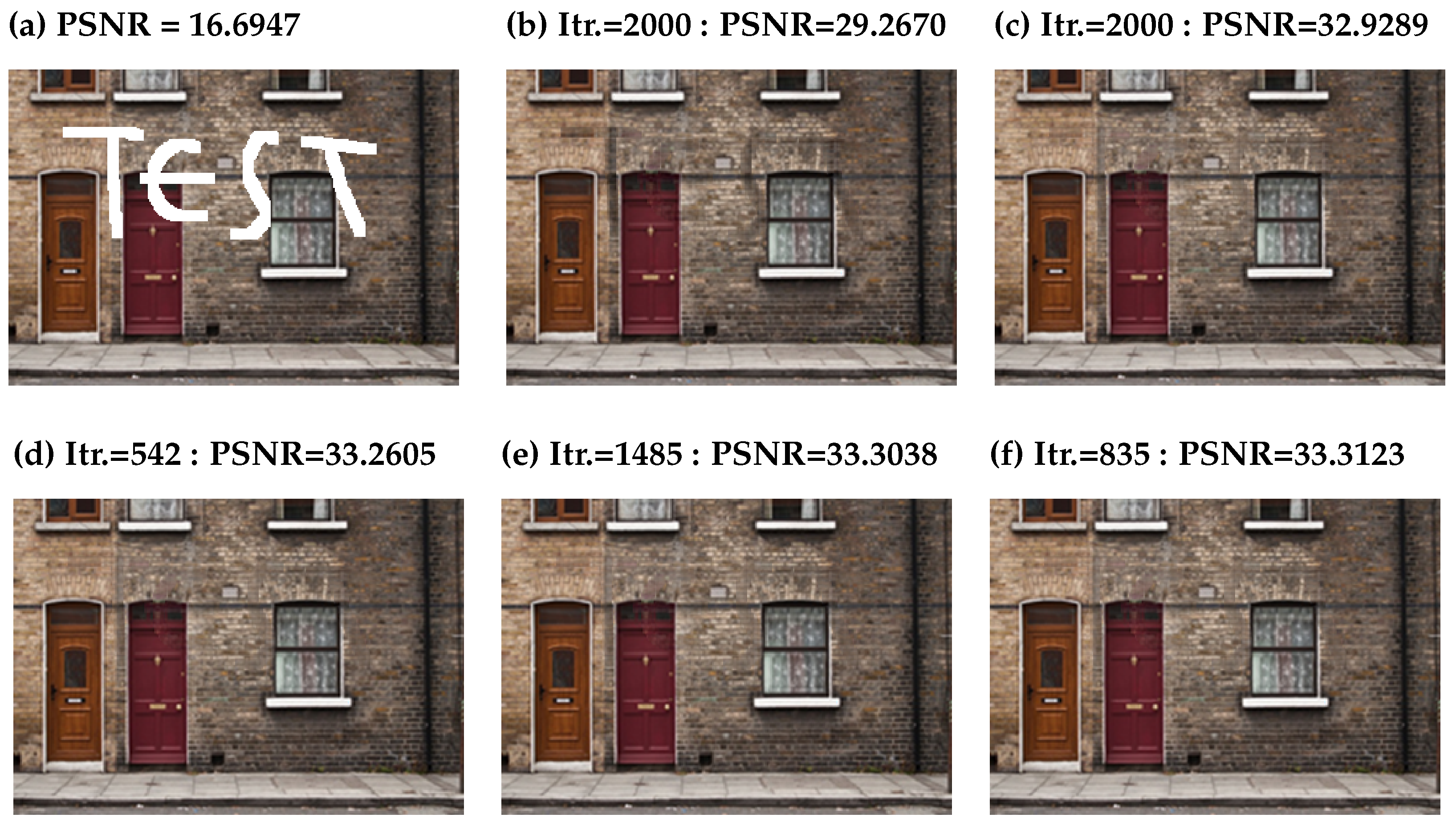
4.1. Image Inpainting Problems

In this experiment, we apply the Algorithm 1 to solving the following constrained image inpainting problems [13]:

$$\underset{z\in \mathcal{C}}{min}{\displaystyle \frac{1}{2}}\parallel {\mathcal{P}}_{\Lambda }\left(z^0\right)-{\mathcal{P}}_{\Lambda }\left(z\right){\parallel }_F^2+\tau {\parallel z\parallel }_{*},$$

(22)

where $z^0\in {\mathbb{R}}^{m\times n}$ is a given image, ${\{z_{ij}^0\}}_{(i,j)\in \Lambda }$ are observed, $\Lambda$ is a subset of the index set $\{1,2,3\dots ,m\}\times \{1,2,3\dots ,n\}$, which indicates where data are available in the image domain and the rest are missed, $\mathcal{C}=\{z\in {\mathbb{R}}^{m\times n}|z_{ij}\ge 0\}$ and define ${\mathcal{P}}_{\Lambda }$ by

$${\mathcal{P}}_{\Lambda }\left(z^0\right)=\left\{\begin{array}{c}{z}_{ij}^0,(i,j)\in \Lambda ,\hfill \\ 0,\mathrm{otherwise}.\hfill \end{array}\right.$$

In Algorithm 1, we set

$${\varphi }_1\left(z\right)={\displaystyle \frac{1}{2}}\parallel {\mathcal{P}}_{\Lambda }\left(z^0\right)-{\mathcal{P}}_{\Lambda }\left(z\right){\parallel }_F^2,{\varphi }_2\left(z\right)=\tau {\parallel z\parallel }_{*},{\omega }_1\left(z\right)=0\mathrm{and}{\omega }_2\left(z\right)={\delta }_{\mathcal{C}}\left(z\right),$$

where $\tau >0$ is regularization parameter, ${\parallel ·\parallel }_F$ is the Frobenius matrix norm and ${\parallel ·\parallel }_{*}$ is the nuclear matrix norm. Then, ${\varphi }_1\left(z\right)$ is convex differentiable and $\nabla {\varphi }_1\left(z\right)={\mathcal{P}}_{\Lambda }\left(z^0\right)-{\mathcal{P}}_{\Lambda }\left(z\right)$ with 1-Lipschitz continuous. We note that the proximity operator of ${\varphi }_2\left(z\right)$ can be computed by the singular value decomposition (SVD), see [26], and the proximity operator of ${\omega }_2\left(z\right)$ is the orthogonal projection onto the closed convex set $\mathcal{C}.$ Therefore, Algorithm 1 is reduced to Algorithm 3 which can be used for solving constrained image inpainting problems (22), we have the following algorithm:

Algorithm 3: Given: $z^0,z^1\in \mathcal{H}.$ Choose $\left\{{\alpha }_k\right\},\left\{{\beta }_k\right\},\left\{{\gamma }_k\right\},$ and $\left\{{\sigma }_k\right\}.$

For$k=1,2,\dots ,$do $$\begin{array}{cc}\hfill w^k& =z^k+{\alpha }_k(z^k-z^{k-1});\hfill \\ \hfill y^k& =w^k+{\beta }_k({\mathrm{prox}}_{{\sigma }_k{\varphi }_2}(\mathcal{I}-{\sigma }_k\nabla {\varphi }_1)w^k-w^k);\hfill \\ \hfill z^{k+1}& =(1-{\gamma }_k){prox}_{{\sigma }_k{\varphi }_2}(\mathcal{I}-{\sigma }_k\nabla {\varphi }_1)w^k+{\gamma }_k{\mathbb{P}}_{\mathcal{C}}{y}^k,\hfill \end{array}$$ end for.

In the standard Gallery, we marked and fixed the damaged portion of the image, and we compared Algorithm 3 with different inertial parameters settings. The following are the details of the parameters for Algorithm 3:

$$\begin{array}{c}\hfill {\beta }_k={\displaystyle \frac{0.9k}{k+1}},{\gamma }_k={\displaystyle \frac{0.01k}{k+1}},{\alpha }_k=\left\{\begin{array}{cc}{\rho }_k\hfill & \mathrm{if}1\le k\le \mathcal{M}\hfill \\ \frac{1}{2^k}\hfill & \mathrm{otherwise},\hfill \end{array}\right.\end{array}$$

where $\mathcal{M}$ is a positive integer depending on the number of iterations of Algorithm 3.

The regularization parameter was set to $\tau =0.01$ and the stopping criterion is as follows:

$${\displaystyle \frac{\parallel z^{k+1}-z^k{\parallel }_F}{\parallel z^k{\parallel }_F}}\le \epsilon ,$$

where $\epsilon$ is a given small constant. The number of iterations is indicated by Iter., and CPU time is indicated by CPU (second). We use the parameters selection cases I–V in

Table 1. The different inertial parameters settings.

Cases	Inertial Parameters
I	${\rho }_k=0$
II	${\rho }_k=0.5$
III	${\rho }_k=0.9$
IV	${\rho }_k=\frac{t_k-1}{t_{k+1}},t_1=1,t_{k+1}=\frac{1+\sqrt{1+4t_k^2}}{2}$
V	${\rho }_k=\frac{k}{k+1}$

to evaluate the performance of Algorithm 3.

Table 2. Results of comparing the selection of inertial parameters in terms of number of iterations, CPU time, PSNR, and the stopping criteria for Algorithm 3.

${\sigma }_{\mathit{k}}$	Inertial Parameters	Iter.	CPU	PSNR (dB)	$\mathsf{\epsilon }$
	Case I	2000	148.6537	23.1486	4.6305 × ${10}^{-5}$
	Case II	2000	148.7307	27.1841	5.4313 × ${10}^{-5}$
0.5	Case III	1225	91.3319	33.1603	9.9616 × ${10}^{-6}$
	Case IV	2000	148.1541	33.3112	1.8945 × ${10}^{-5}$
	Case V	878	65.1786	33.3264	9.9611 × ${10}^{-6}$
	Case I	2000	147.9165	27.1766	5.4335 × ${10}^{-5}$
	Case II	2000	148.2205	32.1462	2.5990 × ${10}^{-5}$
1	Case III	682	50.4207	33.2415	9.9935 × ${10}^{-6}$
	Case IV	1692	125.4178	33.3025	9.9841 × ${10}^{-6}$
	Case V	852	62.9013	33.3276	9.9929 × ${10}^{-6}$
	Case I	2000	150.4054	29.2670	4.8888 × ${10}^{-5}$
	Case II	2000	147.7252	32.9289	1.2150 × ${10}^{-5}$
1.3	Case III	542	40.1375	33.2605	9.9835 × ${10}^{-6}$
	Case IV	1485	109.8176	33.3038	9.9924 × ${10}^{-6}$
	Case V	835	61.5336	33.3123	9.9484 × ${10}^{-6}$

displays the results that were achieved. We observe from Table 2 that when the stopping criterion $\epsilon ={10}^{-5}$ or at the 2000th iteration, Algorithm 3 with inertial parameter (Case V) outperforms the other cases in terms of PSNR performance. We may infer from Table 2 that Algorithm 3 is more effective at recovering images when inertial parameters are added. The test image and the restored images are shown in Figure 1 and Figure 2.

To solve a general convex optimization problem, model the sum of three convex functions in the form:

$$\underset{x\in \mathcal{H}}{min}{\varphi }_1\left(x\right)+{\varphi }_2\left(x\right)+{\varphi }_3\left(x\right),$$

(23)

where ${\varphi }_1:\mathcal{H}\to \mathbb{R},{\varphi }_2:\mathcal{H}\to \mathbb{R}\cup \{\infty \}$ and ${\varphi }_3:\mathcal{H}\to \mathbb{R}\cup \{\infty \}$ are convex and proper lower semi-continuous function and ${\varphi }_1$ is a differentiable function with a $\mathcal{L}$-Lipschitz continuous gradient. Cui et al. introduced an inertial three-operator splitting (iTOS) algorithm [13] which can be applied to solving constrained image inpainting problems (22).

Next experiment, we set ${\varphi }_1\left(z\right)={\displaystyle \frac{1}{2}}\parallel {\mathcal{P}}_{\Lambda }\left(z^0\right)-{\mathcal{P}}_{\Lambda }\left(z\right){\parallel }_F^2,{\varphi }_2\left(z\right)=\tau {\parallel z\parallel }_{*},\mathrm{and}{\varphi }_3\left(z\right)={\delta }_{\mathcal{C}}\left(z\right),$ for Algorithm 4 (iTOS algorithm) and use the parameters selection as in

Table 3. Results of comparing the selection of parameters in terms of number of iterations, CPU time, PSNR, and the stopping criteria for iTOS algorithm.

${\sigma }_{\mathit{k}}$	Parameters	Iter.	CPU	PSNR (dB)	$\mathsf{\epsilon }$
	${\alpha }_k=0.1,{\beta }_k=1.4$	2000	150.3057	25.3434	5.5297 × ${10}^{-5}$
	${\alpha }_k=0.2,{\beta }_k=0.8$	2000	152.3218	23.0876	4.6797 × ${10}^{-5}$
0.5	${\alpha }_k=0.5,{\beta }_k=0.3$	2000	151.0935	21.4506	3.5078 × ${10}^{-5}$
	${\alpha }_k=0.8,{\beta }_k=0.4$	2000	161.5143	27.0492	5.5804 × ${10}^{-5}$
	${\alpha }_k=0.9,{\beta }_k=0.5$	2000	163.1106	30.4406	3.9901 × ${10}^{-5}$
	${\alpha }_k=0.1,{\beta }_k=1.4$	2000	150.6947	30.2252	4.7538 × ${10}^{-5}$
	${\alpha }_k=0.2,{\beta }_k=0.8$	2000	150.9510	27.0585	5.5603 × ${10}^{-5}$
1	${\alpha }_k=0.5,{\beta }_k=0.3$	2000	164.3304	23.9033	5.0955 × ${10}^{-5}$
	${\alpha }_k=0.8,{\beta }_k=0.4$	2000	156.7255	30.9755	4.0485 × ${10}^{-5}$
	${\alpha }_k=0.9,{\beta }_k=0.5$	2000	158.6223	25.3198	7.2758 × ${10}^{-5}$
	${\alpha }_k=0.1,{\beta }_k=1.4$	2000	149.7497	30.9921	4.0100 × ${10}^{-5}$
	${\alpha }_k=0.2,{\beta }_k=0.8$	2000	151.2015	29.0476	5.2936 × ${10}^{-5}$
1.3	${\alpha }_k=0.5,{\beta }_k=0.3$	2000	153.6181	25.3584	5.5326 × ${10}^{-6}$
	${\alpha }_k=0.8,{\beta }_k=0.4$	2000	155.3317	30.3421	3.9970 × ${10}^{-5}$
	${\alpha }_k=0.9,{\beta }_k=0.5$	2000	155.7551	22.9716	9.3178 × ${10}^{-5}$

to evaluate the performance. Table 3 displays the results that were achieved. We observe from Table 2 and Table 3 that when the stopping criterion $\epsilon ={10}^{-5}$ or at the 2000th iteration, the Algorithm 3 with inertial parameter (Case V) outperforms all cases of the iTOS algorithm in terms of PSNR performance.

Algorithm 4: An inertial three-operator splitting (iTOS) algorithm [13].

Let $z^0,z^1\in \mathcal{H}$ and $\lambda \in (0,\frac{2}{\mathcal{L}}\overline{\epsilon }),$ where $\overline{\epsilon }\in (0,1).$ For $k\ge 1$, let $$\begin{array}{cc}\hfill w^k& =z^k+{\alpha }_k(z^k-z^{k-1});\hfill \\ \hfill y_{{\varphi }_3}^k& ={prox}_{\lambda {\varphi }_3}{w}^k;\hfill \\ \hfill y_{{\varphi }_2}^k& ={prox}_{\lambda {\varphi }_2}(2y_{{\varphi }_3}^k-y^k-\lambda \nabla {\varphi }_1\left(y_{{\varphi }_3}^k\right));\hfill \\ \hfill z^{k+1}& =w^k+{\beta }_k(y_{{\varphi }_2}^k-y_{{\varphi }_3}^k),\hfill \end{array}$$   where $\left\{{\alpha }_k\right\}$ is nondecreasing with $k\ge 1,$$0\le {\alpha }_k\le \alpha <1$ and for all $k\ge 1,$ and   $\beta ,a,b>0$ such that $$\begin{array}{c}b>{\displaystyle \frac{{\alpha }^2(1+\alpha )+\alpha a}{1-{\alpha }^2}}\mathrm{and}0<\beta \le {\beta }_k\le {\displaystyle \frac{b-\alpha \left[\alpha \right(1+\alpha )+\alpha b+a]}{\overline{\alpha }b[1+\alpha (1+\alpha )+\alpha b+a]}},\mathrm{where}\overline{\alpha }={\displaystyle \frac{1}{2-\overline{\epsilon }}}.\hfill \end{array}$$

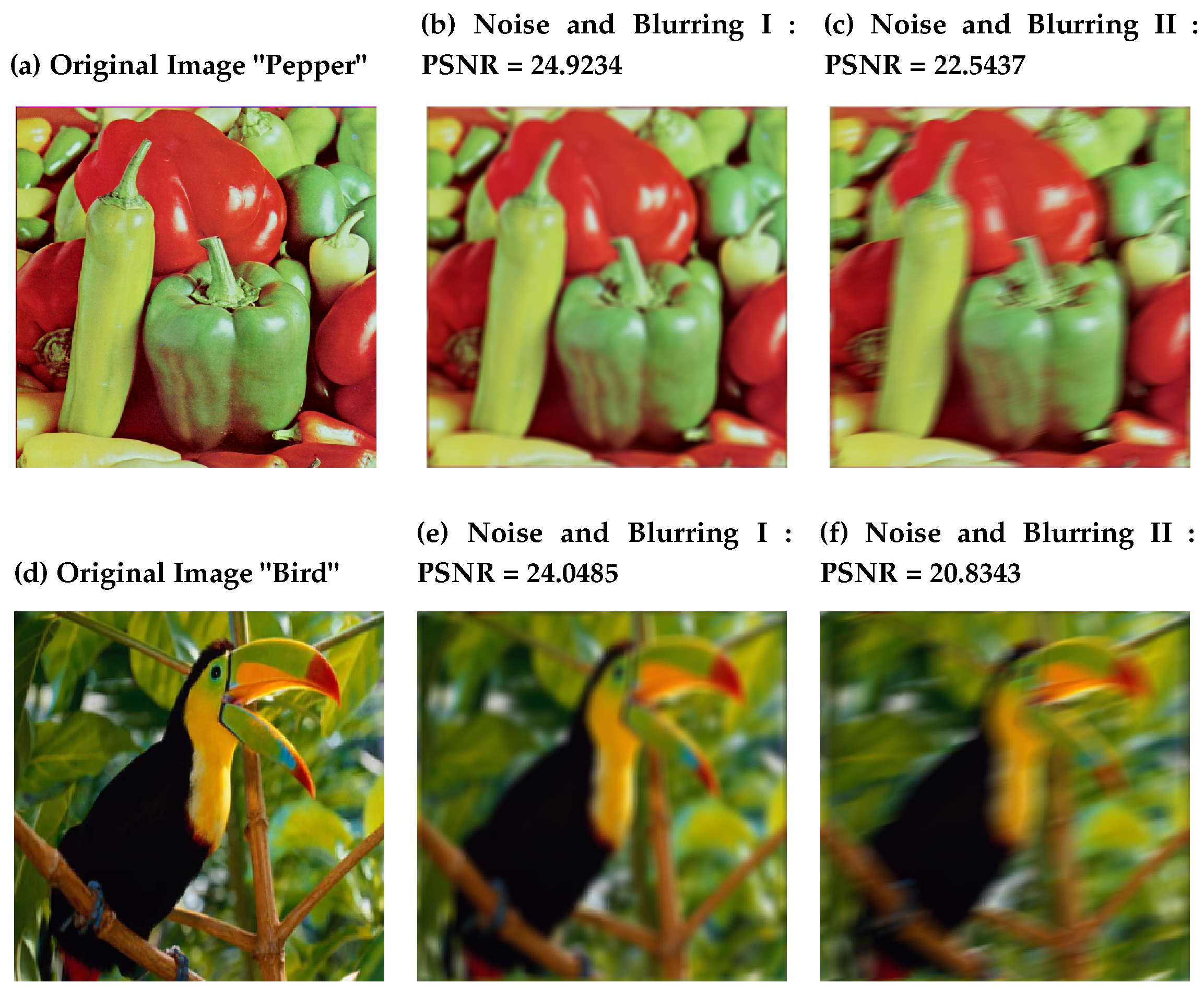
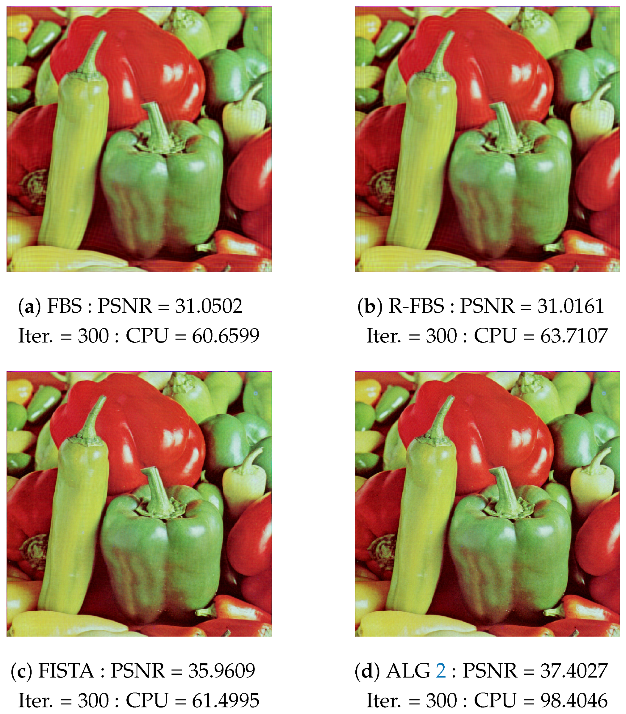
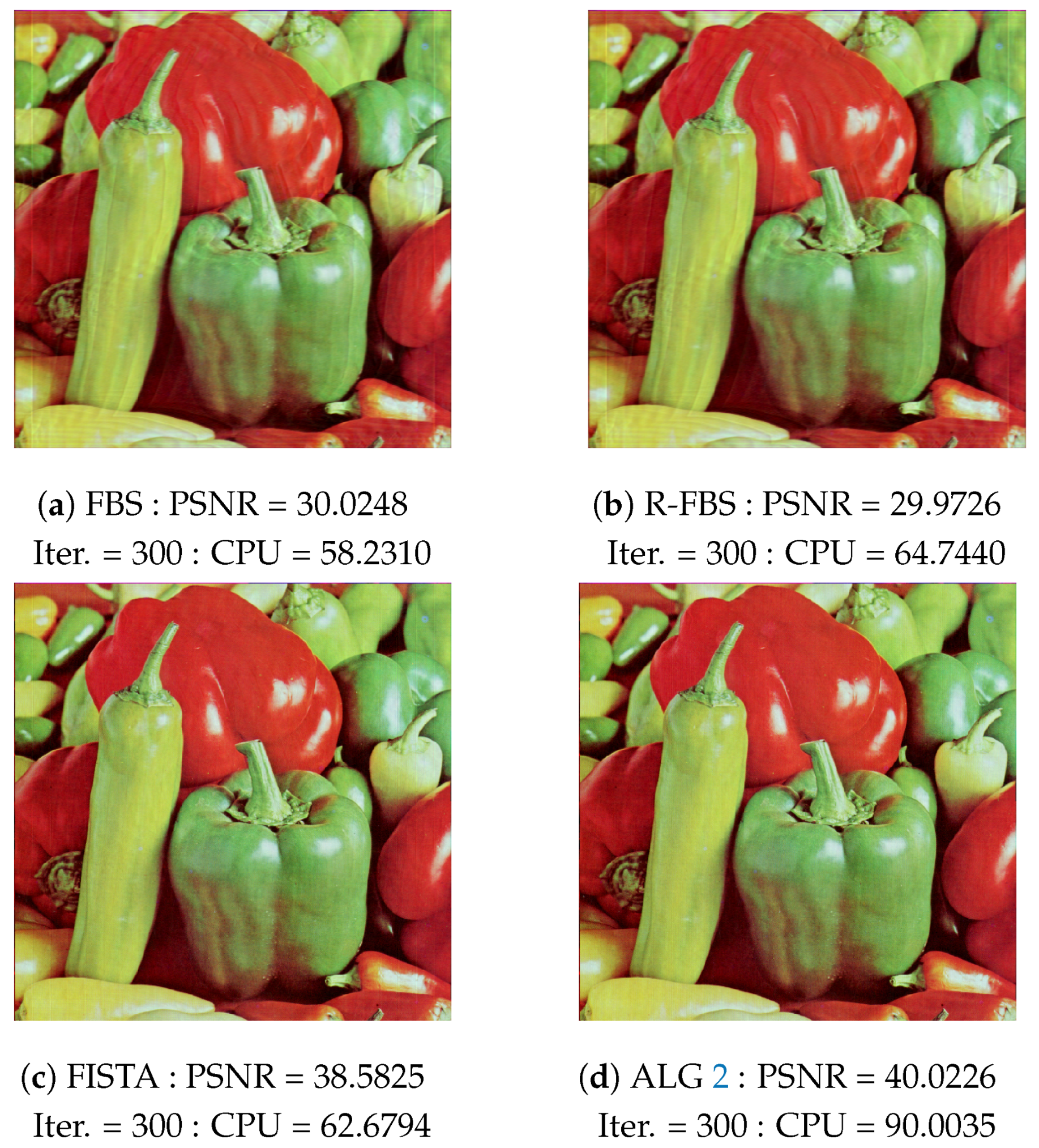
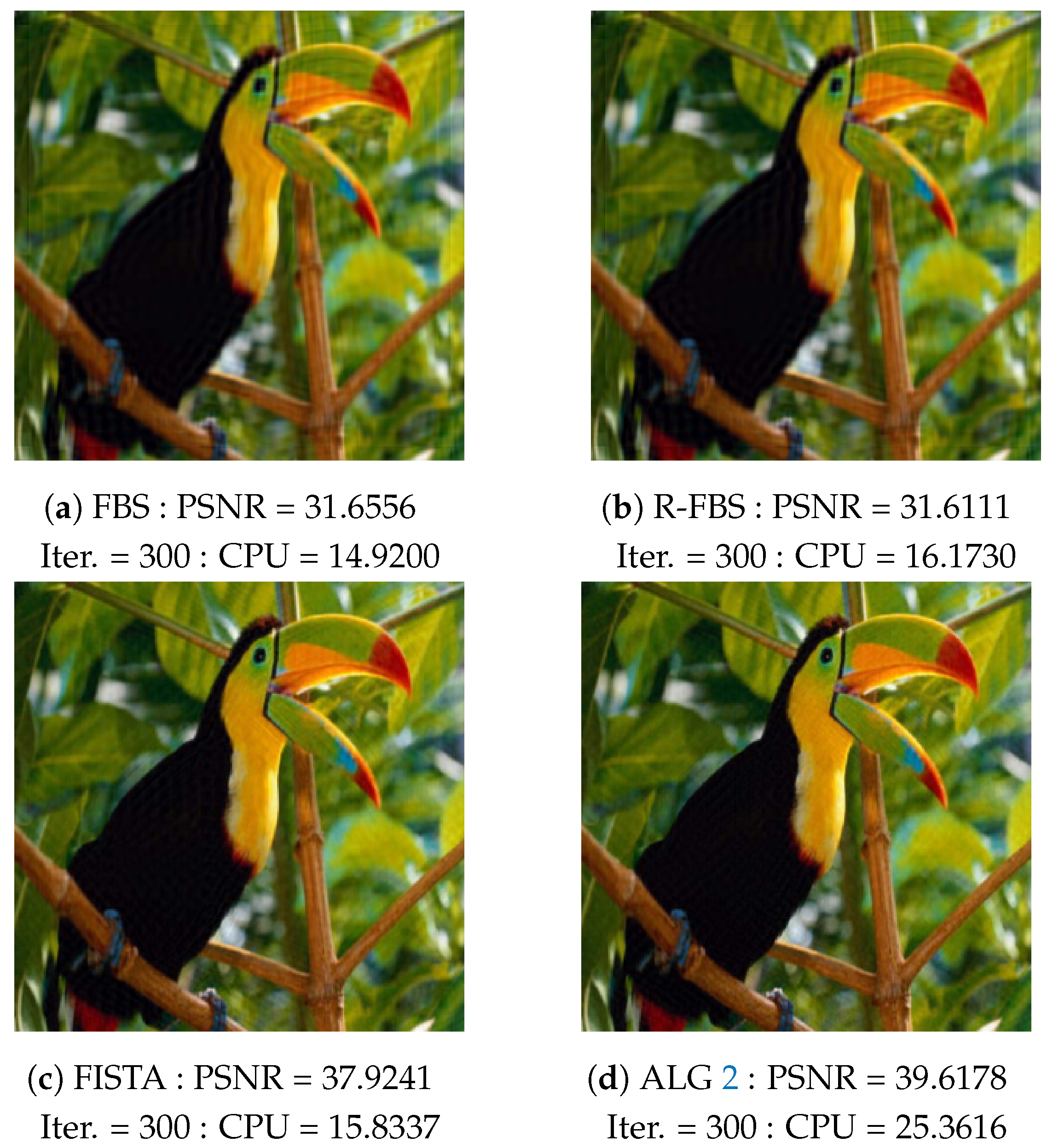
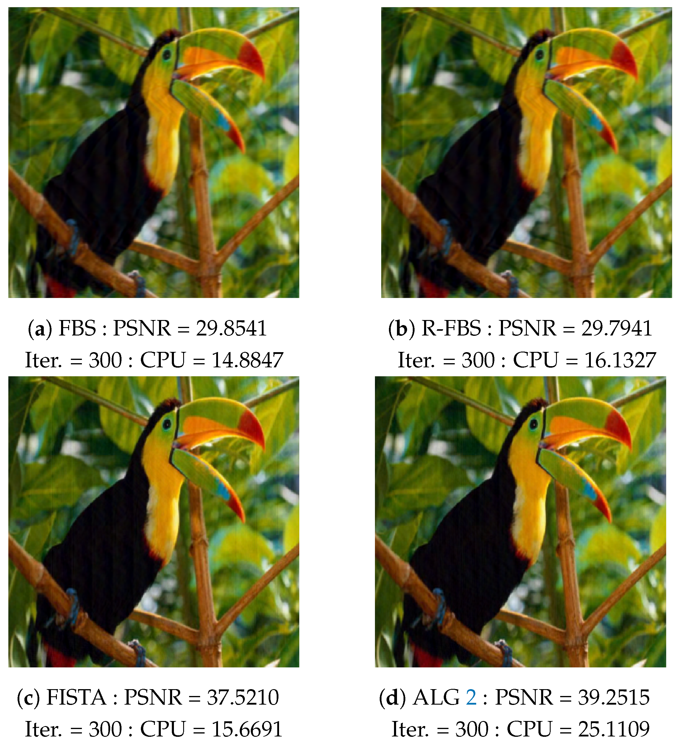
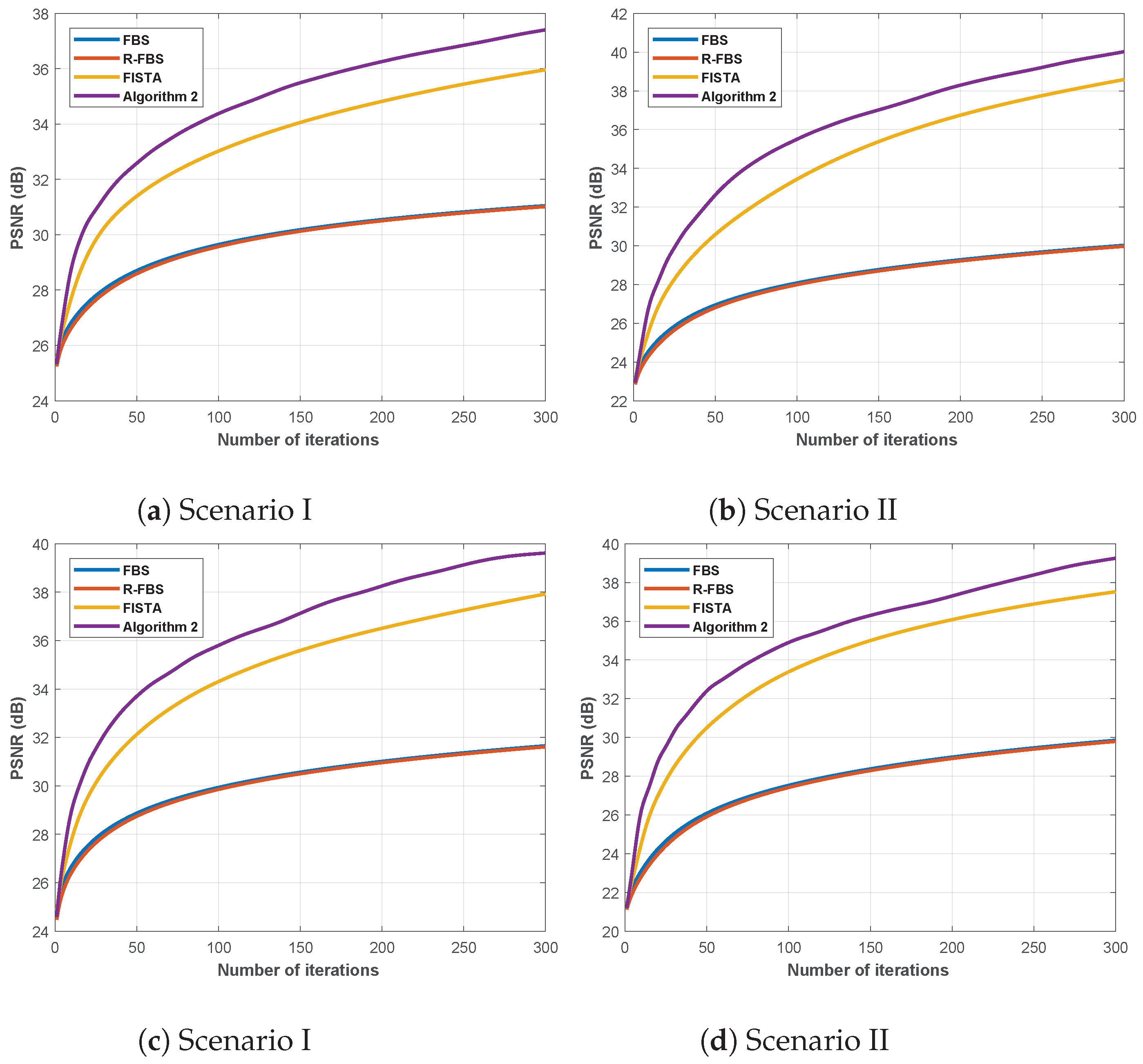
4.2. Image Restoration Problems

In this experiment, we apply the Algorithm 2 to solving the image restoration problems by using the LASSO model [25]:

$$\underset{z\in {\mathbb{R}}^N}{min}\left\{\frac{1}{2}{∥Bz-ϵ∥}_2^2+\tau {\parallel z\parallel }_1\right\},$$

(24)

where $\tau >0$, ${\parallel ·\parallel }_1$ is the $l_1$-norm and ${\parallel ·\parallel }_2$ is the Euclidean norm.

In Algorithm 2, we set ${\varphi }_1\left(z\right)=\frac{1}{2}{∥ϵ-Bz∥}_2^2\mathrm{and}{\varphi }_2\left(z\right)=\tau {\parallel z\parallel }_1,$ where $ϵ$ is the observed image and $B=RW$, when R and W are the kernel matrix and 2-D fast Fourier transform, respectively.

We will use two test photos (Pepper and Bird, with sizes of $512\times 512$ and $288\times 288$, respectively) to exhibit two scenarios of blurring processes in

Table 4. Processes of blurring in Detail.

Scenarios	Kernel Matrix
I	Gaussian blur of filter size $9\times 9$ with standard deviation $\widehat{\sigma }=17$
II	Motion blur specifying with motion length of 21 pixels and motion orientation $15°$

and add a random Gaussian white noise ${10}^{-5}$, with the original and blurred images shown in Figure 3.

We examine and compare the efficiency of our algorithms (Algorithm 2 := ALG 2) to that of FBS, R-FBS and FISTA algorithms. The image restoration performance of the examined methods is next tested by setting as described in (25) and using blurred images as starting points. For all algorithms, the maximum number of iterations is set at 300. The regularization parameter in the LASSO model (24) is set to $\tau ={10}^{-5}$. The following are the parameters for the studied algorithms under consideration:

$$\begin{array}{c}\hfill {\sigma }_k=\frac{1}{\mathcal{L}},{\beta }_k={\gamma }_k={\displaystyle \frac{0.99k}{k+1}},{\alpha }_k=\left\{\begin{array}{cc}\frac{k}{k+1}\hfill & \mathrm{if}1\le k\le \mathcal{M}\hfill \\ \frac{1}{2^k}\hfill & \mathrm{otherwise},\hfill \end{array}\right.\end{array}$$

(25)

where $\mathcal{M}$ is a positive integer depending on the number of iteration of Algorithm 2.

Figure 4, Figure 5, Figure 6 and Figure 7 present the deblurring test images by the studied algorithms. In Figure 8, we see that the graph of PSNR of Algorithm 2 is higher than the others, which means that the efficiency of restored images by Algorithm 2 is better than the other methods. The number of iterations is indicated by Iter., and CPU time is indicated by CPU (second).

5. Conclusions

In this research, an inertial forward-backward splitting algorithm for solving a common point of convex minimization problems is developed. We investigated the weak convergence of the suggested algorithm based on the fixed point equation of the forward-backward operator under some suitable control conditions. Finally, we use numerical simulations to show the benefits of the inertial terms in the studied algorithms for the constrained image inpainting problems (22) and the image restoration problems (24).

References

1. Bertsekas, D.P.; Tsitsiklis, J.N. Parallel and Distributed Computation: Numerical Methods; Athena Scientific: Belmont, MA, USA, 1997. [Google Scholar]
2. Combettes, P.L.; Pesquet, J.C. A Douglas-Rachford splitting approach to nonsmooth convex variational signal recovery. IEEE J. Sel. Top. Signal Process. 2007, 1, 564–574. [Google Scholar] [CrossRef]
3. Combettes, P.L.; Wajs, V.R. Signal recovery by proximal forward-backward splitting. Multiscale Model. Simul. 2005, 4, 1168–1200. [Google Scholar] [CrossRef] [Green Version]
4. Hanjing, A.; Suantai, S. An inertial alternating projection algorithm for convex minimization problems with applications to signal recovery problems. J. Nonlinear Convex Anal. 2022, 22, 2647–2660. [Google Scholar]
5. Lin, L.J.; Takahashi, W. A general iterative method for hierarchical variational inequality problems in Hilbert spaces and applications. Positivity 2012, 16, 429–453. [Google Scholar] [CrossRef]
6. Lions, P.L.; Mercier, B. Splitting algorithms for the sum of two nonlinear operators. SIAM J. Numer. Anal. 1979, 16, 964–979. [Google Scholar] [CrossRef]
7. Martinet, B. Régularisation d’inéquations variationnelles par approximations successives. Rev. Fr. D’Inform. Rech. Oper. 1970, 4, 154–158. [Google Scholar]
8. Yatakoat, P.; Suantai, S.; Hanjing, A. On some accelerated optimization algorithms based on fixed point and linesearch techniques for convex minimization problems with applications. Adv. Contin. Discret. Model. 2022, 25. [Google Scholar] [CrossRef]
9. Suantai, S.; Jailoka, P.; Hanjing, A. An accelerated viscosity forward-backward splitting algorithm with the linesearch process for convex minimization problems. J. Inequal. Appl. 2021, 42. [Google Scholar] [CrossRef]
10. Rockafellar, R.T. Monotone operators and the proximal point algorithm. SIAM J. Control Optim. 1976, 17, 877–898. [Google Scholar] [CrossRef] [Green Version]
11. Aremu, K.O.; Izuchukwu, C.; Grace, O.N.; Mewomo, O.T. Multi-step iterative algorithm for minimization and fixed point problems in p-uniformly convex metric spaces. J. Ind. Manag. Optim. 2020, 13, 2161–2180. [Google Scholar] [CrossRef] [Green Version]
12. Bot, R.I.; Csetnek, E.R.; Hendrich, C. Inertial Douglas-Rachford splitting for monotone inclusion problems. Appl. Math. Comput. 2015, 256, 472–487. [Google Scholar] [CrossRef] [Green Version]
13. Cui, F.; Tang, Y.; Yang, Y. An inertial three-operator splitting algorithm with applications to image inpainting. arXiv 2019, arXiv:1904.11684. [Google Scholar]
14. Hanjing, A.; Suantai, S. A fast image restoration algorithm based on a fixed point and optimization. Mathematics 2020, 8, 378. [Google Scholar] [CrossRef]
15. Thongpaen, P.; Wattanataweekul, R. A fast fixed-point algorithm for convex minimization problems and its application in image restoration problems. Mathematics 2021, 9, 2619. [Google Scholar] [CrossRef]
16. Suantai, S.; Kankam, K.; Cholamjiak, P. A novel forward-backward algorithm for solving convex minimization problem in Hilbert spaces. Mathematics 2020, 8, 42. [Google Scholar] [CrossRef] [Green Version]
17. Beck, A.; Teboulle, M. A fast iterative shrinkage-thresholding algorithm for linear inverse problems. SIAM J. Imaging Sci. 2009, 2, 183–202. [Google Scholar] [CrossRef] [Green Version]
18. Bussaban, L.; Suantai, S.; Kaewkhao, A. A parallel inertial S-iteration forward-backward algorithm for regression and classification problems. Carpathian J. Math. 2020, 36, 35–44. [Google Scholar] [CrossRef]
19. Burachik, R.S.; Iusem, A.N. Set-Valued Mappings and Enlargements of Monotone Operator; Springer Science Business Media: New York, NY, USA, 2007. [Google Scholar]
20. Opial, Z. Weak convergence of the sequence of successive approximations for nonexpansive mappings. Bull. Am. Math. Soc. 1967, 73, 591–597. [Google Scholar] [CrossRef] [Green Version]
21. Nakajo, K.; Shimoji, K.; Takahashi, W. On strong convergence by the hybrid method for families of mappings in Hilbert spaces. Nonlinear Anal. Theory Methods Appl. 2009, 71, 112–119. [Google Scholar] [CrossRef]
22. Bauschke, H.H.; Combettes, P.L. Convex Analysis and Monotone Operator Theory in Hilbert Spaces; Springer: New York, NY, USA, 2011. [Google Scholar]
23. Tan, K.; Xu, H.K. Approximating fixed points of nonexpansive mappings by the ishikawa iteration process. J. Math. Anal. Appl. 1993, 178, 301–308. [Google Scholar] [CrossRef] [Green Version]
24. Moudafi, A.; Al-Shemas, E. Simultaneous iterative methods for split equality problem. Trans. Math. Program. Appl. 2013, 1, 1–11. [Google Scholar] [CrossRef] [Green Version]
25. Thung, K.; Raveendran, P. A survey of image quality measures. In Proceedings of the International Conference for Technical Postgraduates (TECHPOS), Kuala Lumpur, Malaysia, 14–15 December 2009; pp. 1–4. [Google Scholar]
26. Cai, J.F.; Candes, E.J.; Shen, Z. A singular value thresholding algorithm for matrix completion. SIAM J. Optim. 2010, 20, 1956–1982. [Google Scholar] [CrossRef]
Figure 1. Test image.
Symmetry 15 00007 g001
Figure 2. The painted image and restored images. (a) The painted image; (bf) Images that have been recovered for cases I through V with σ k = 1.3 , respectively.
Symmetry 15 00007 g002
Figure 3. The deblurring images of Pepper and Bird.
Symmetry 15 00007 g003
Figure 4. The PSNR, Iter. and CPU of the FBS, R-FBS, FISTA and ALG 2 for scenario I of the Pepper.
Symmetry 15 00007 g004
Figure 5. The PSNR, Iter. and CPU of the FBS, R-FBS, FISTA and ALG 2 for scenario II of the Pepper.
Symmetry 15 00007 g005
Figure 6. The PSNR, Iter. and CPU of the FBS, R-FBS, FISTA and ALG 2 for scenario I of the Bird.
Symmetry 15 00007 g006
Figure 7. The PSNR, Iter. and CPU of the FBS, R-FBS, FISTA and ALG 2 for scenario II of the Bird.
Symmetry 15 00007 g007
Figure 8. The PSNR graphs of the studied algorithms: (a,b) for Pepper; (c,d) for Bird.
Symmetry 15 00007 g008