Figure 1.
The relationship between L and “a” when “b” = 0.25, 0.50.
Figure 1.
The relationship between L and “a” when “b” = 0.25, 0.50.
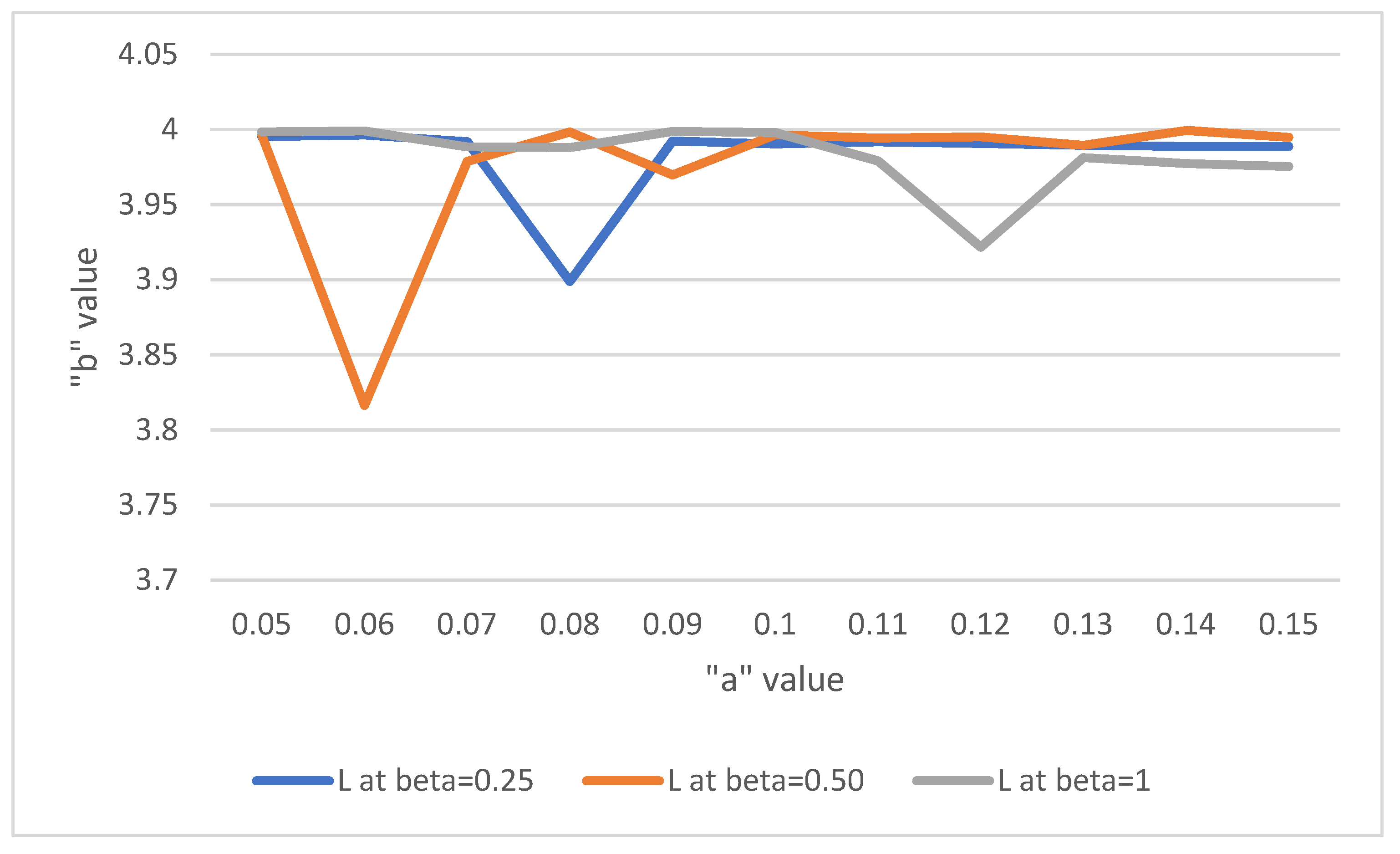
Figure 2.
The relationship between L and “a” when “b” = 0.25, 0.50, 1.
Figure 2.
The relationship between L and “a” when “b” = 0.25, 0.50, 1.
Figure 3.
The relationship between L and “a” when “b” = 0.25, 0.50, 1.
Figure 3.
The relationship between L and “a” when “b” = 0.25, 0.50, 1.
Figure 4.
The relationship between L and “a” when “b” = 0.25, 0.50, 1.
Figure 4.
The relationship between L and “a” when “b” = 0.25, 0.50, 1.
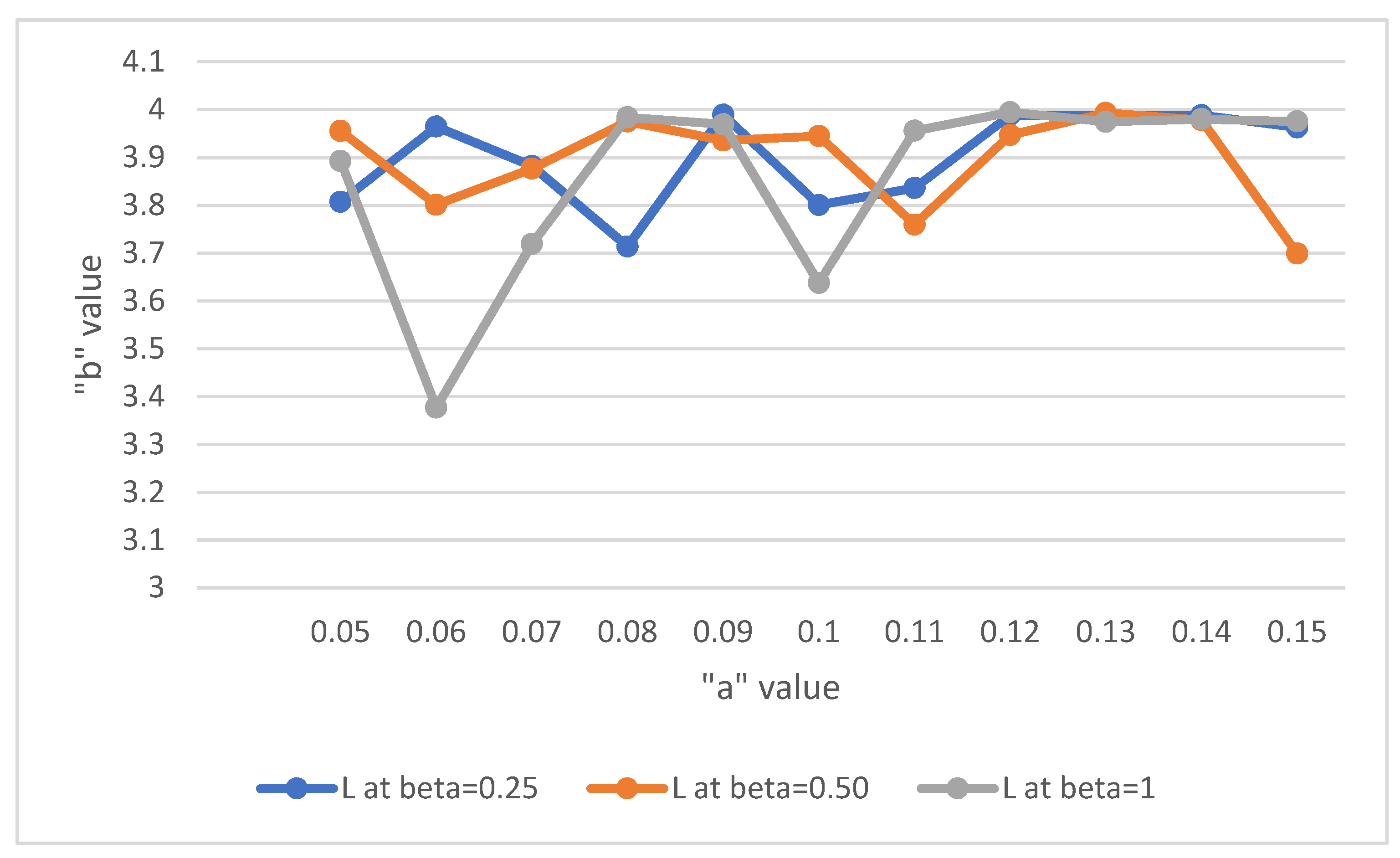
Figure 5.
The relationship between L and “a” when “b” = 0.25, 0.50, 1.
Figure 5.
The relationship between L and “a” when “b” = 0.25, 0.50, 1.
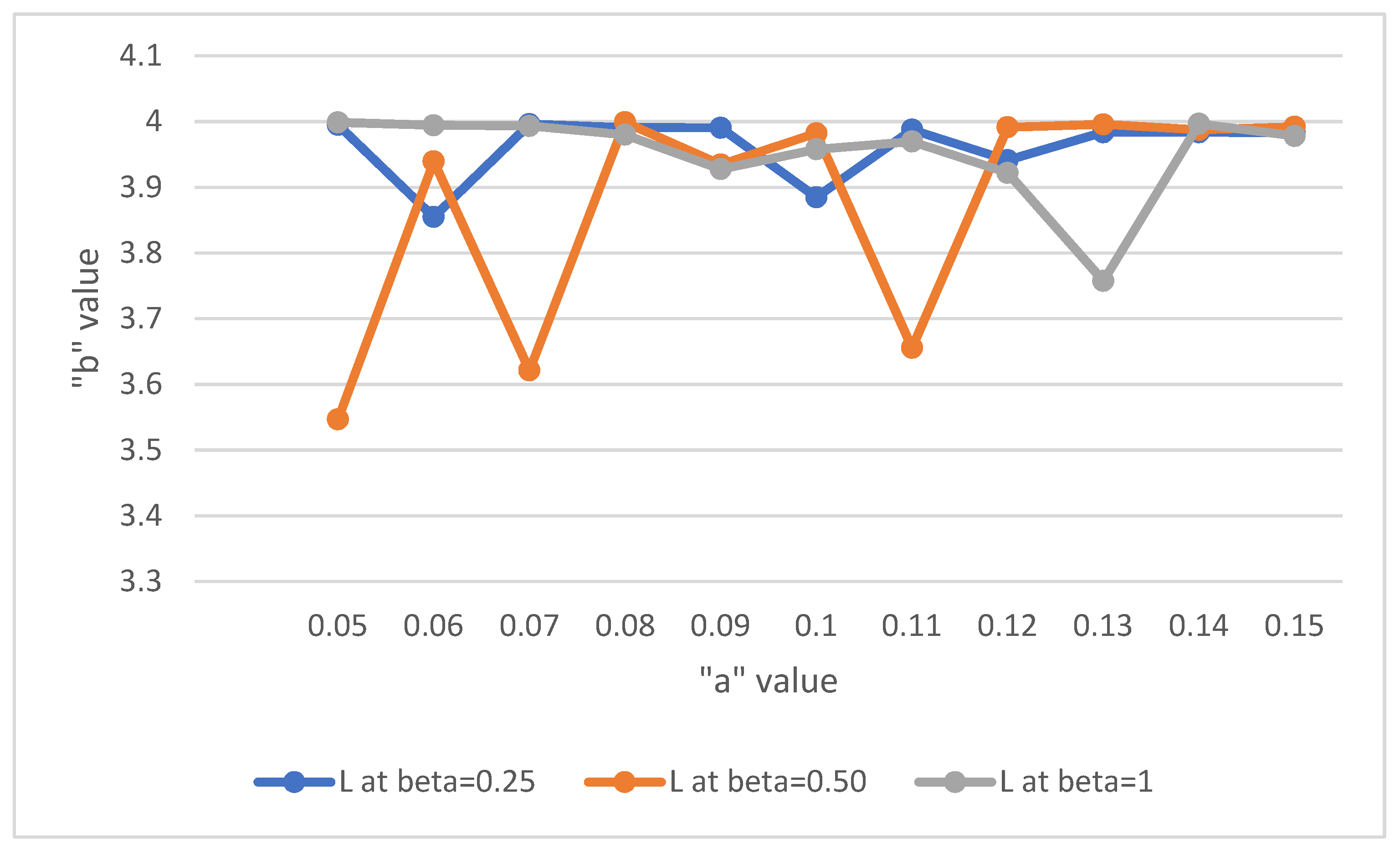
Figure 6.
The relationship between L and “a” when “b” = 0.25, 0.50, 1.
Figure 6.
The relationship between L and “a” when “b” = 0.25, 0.50, 1.
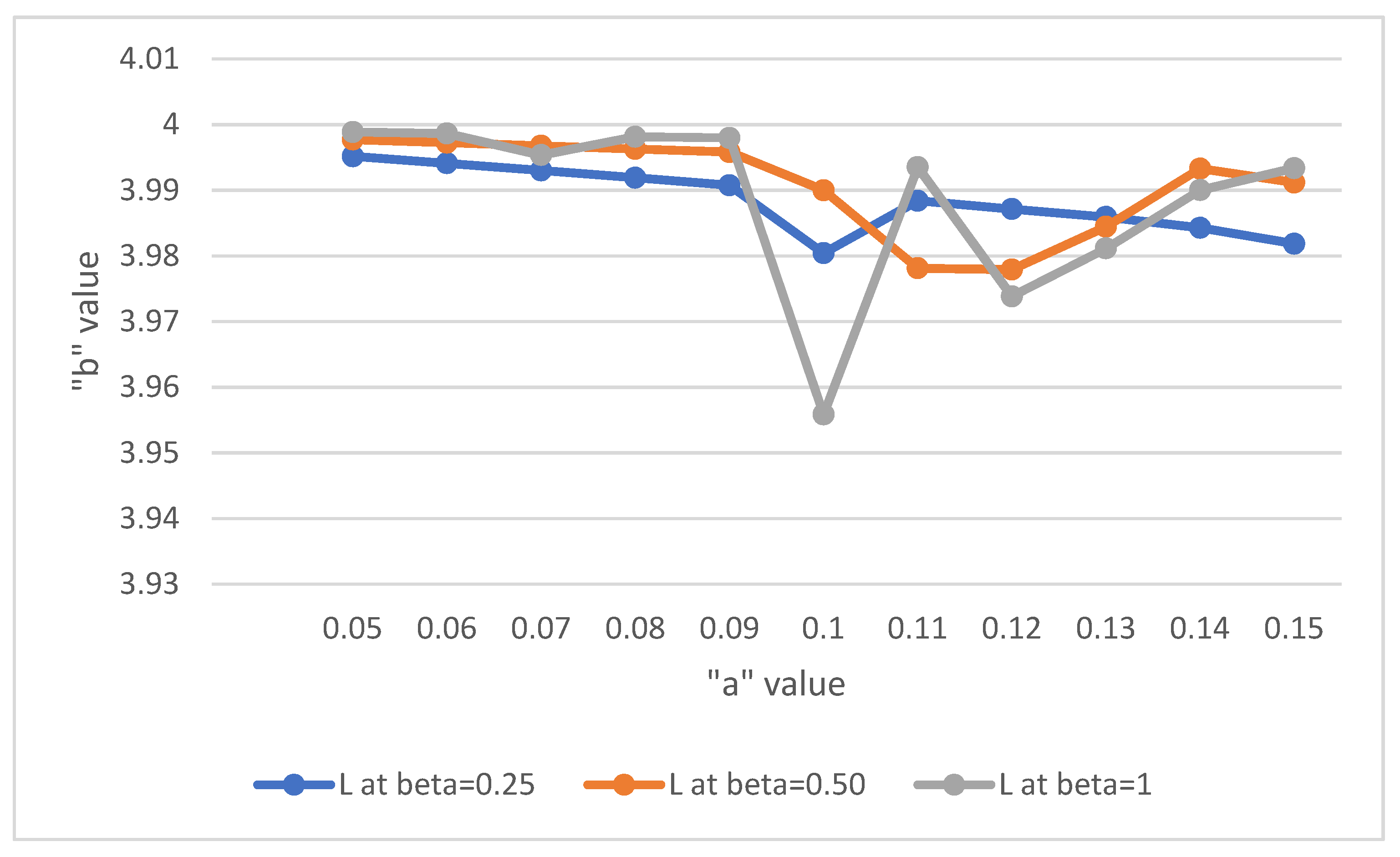
Figure 7.
The relationship between L and “a” when “b” = 0.25, 0.50, 1.
Figure 7.
The relationship between L and “a” when “b” = 0.25, 0.50, 1.
Table 1.
The values of L for different values of b = 0.25, 0.50, 1.
Table 1.
The values of L for different values of b = 0.25, 0.50, 1.
| a | L at b = 0.25 | L at b = 0.50 | L at b = 1 |
|---|
| 0.05 | 3.995225 | 3.996138 | 3.998365 |
| 0.06 | 3.996334 | 3.816372 | 3.999065 |
| 0.07 | 3.991855 | 3.978771 | 3.988408 |
| 0.08 | 3.898826 | 3.998237 | 3.988041 |
| 0.09 | 3.992406 | 3.969705 | 3.998728 |
| 0.10 | 3.972794 | 3.996458 | 3.997931 |
| 0.11 | 3.991761 | 3.994401 | 3.979199 |
| 0.12 | 3.990751 | 3.995094 | 3.921691 |
| 0.13 | 3.989561 | 3.989560 | 3.981316 |
| 0.14 | 3.988700 | 3.999407 | 3.977291 |
| 0.15 | 3.988784 | 3.994852 | 3.975339 |
Table 2.
Comparison of L-Expected number of units in the system between poisson and encouraged arrival.
Table 2.
Comparison of L-Expected number of units in the system between poisson and encouraged arrival.
| a | Poisson Arrival
L at b = 0.50 | Encouraged Arrival
L at b = 0.50 |
|---|
| 0.06 | 3.967179 | 3.816372 |
Table 3.
Comparison of L-Expected number of units in the system between poisson and encouraged arrival.
Table 3.
Comparison of L-Expected number of units in the system between poisson and encouraged arrival.
| a | Poisson Arrival
L at b = 1 | Encouraged Arrival
L at b = 1 |
|---|
| 0.08 | 3.985963 | 3.988041 |
| 0.11 | 3.980742 | 3.979199 |
| 0.12 | 3.979004 | 3.921691 |
Table 4.
Verification of Little’s law.
Table 4.
Verification of Little’s law.
| S.No | b | a | L | W | L/W | λ |
|---|
| 1 | 0.25 | 0.05 | 3.995225 | 0.66587083 | 5.999998498 | 6 |
| 2 | 0.5 | 0.05 | 3.996334 | 0.66605567 | 5.999996997 | 6 |
| 3 | 1 | 0.05 | 3.998365 | 0.66639417 | 6.000001501 | 6 |
| 4 | 0.25 | 0.06 | 3.996334 | 0.66605567 | 5.999996997 | 6 |
| 5 | 0.5 | 0.06 | 3.816372 | 0.63606200 | 6 | 6 |
| 6 | 1 | 0.06 | 3.999065 | 0.66651083 | 5.9999985 | 6 |
| 7 | 0.25 | 0.07 | 3.991855 | 0.66531417 | 5.999956412 | 6 |
| 8 | 0.5 | 0.07 | 3.978771 | 0.66312850 | 5.999995476 | 6 |
| 9 | 1 | 0.07 | 3.988408 | 0.66473467 | 5.999996991 | 6 |
| 10 | 0.25 | 0.08 | 3.898826 | 0.64980433 | 6.000003078 | 6 |
| 11 | 0.5 | 0.08 | 3.998237 | 0.66637283 | 5.999998499 | 6 |
| 12 | 1 | 0.08 | 3.988041 | 0.66467350 | 5.999995487 | 6 |
| 13 | 0.25 | 0.09 | 3.992406 | 0.6654010 | 6 | 6 |
| 14 | 0.5 | 0.09 | 3.969705 | 0.6616175 | 5.999995466 | 6 |
| 15 | 1 | 0.09 | 3.998728 | 0.6664546 | 5.999996999 | 6 |
| 16 | 0.25 | 0.1 | 3.972794 | 0.6621323 | 6.000003021 | 6 |
| 17 | 0.5 | 0.1 | 3.996458 | 0.6660763 | 6.000003003 | 6 |
| 18 | 1 | 0.1 | 3.997931 | 0.6663218 | 5.999998499 | 6 |
| 19 | 0.25 | 0.11 | 3.991761 | 0.6652935 | 5.999995491 | 6 |
| 20 | 0.5 | 0.11 | 3.994401 | 0.6657335 | 5.999995494 | 6 |
| 21 | 1 | 0.11 | 3.979199 | 0.6631998 | 5.999998492 | 6 |
| 22 | 0.25 | 0.12 | 3.990751 | 0.6651251 | 6.000001503 | 6 |
| 23 | 0.5 | 0.12 | 3.995094 | 0.6658490 | 6 | 6 |
| 24 | 1 | 0.12 | 3.921691 | 0.6536151 | 6.00000153 | 6 |
| 25 | 0.25 | 0.13 | 3.989561 | 0.6649268 | 5.999998496 | 6 |
| 26 | 0.5 | 0.13 | 3.989560 | 0.6649266 | 5.999996992 | 6 |
| 27 | 1 | 0.13 | 3.981316 | 0.6635526 | 5.999996986 | 6 |
| 28 | 0.25 | 0.14 | 3.988700 | 0.6647833 | 6.000003009 | 6 |
| 29 | 0.5 | 0.14 | 3.999407 | 0.6665678 | 5.9999985 | 6 |
| 30 | 1 | 0.14 | 3.977291 | 0.6628818 | 5.999998491 | 6 |
| 31 | 0.25 | 0.15 | 3.988784 | 0.6647973 | 6.000030085 | 6 |
| 32 | 0.5 | 0.15 | 3.994852 | 0.6658086 | 5.999996996 | 6 |
| 33 | 1 | 0.15 | 3.975339 | 0.6625560 | 5.999995472 | 6 |
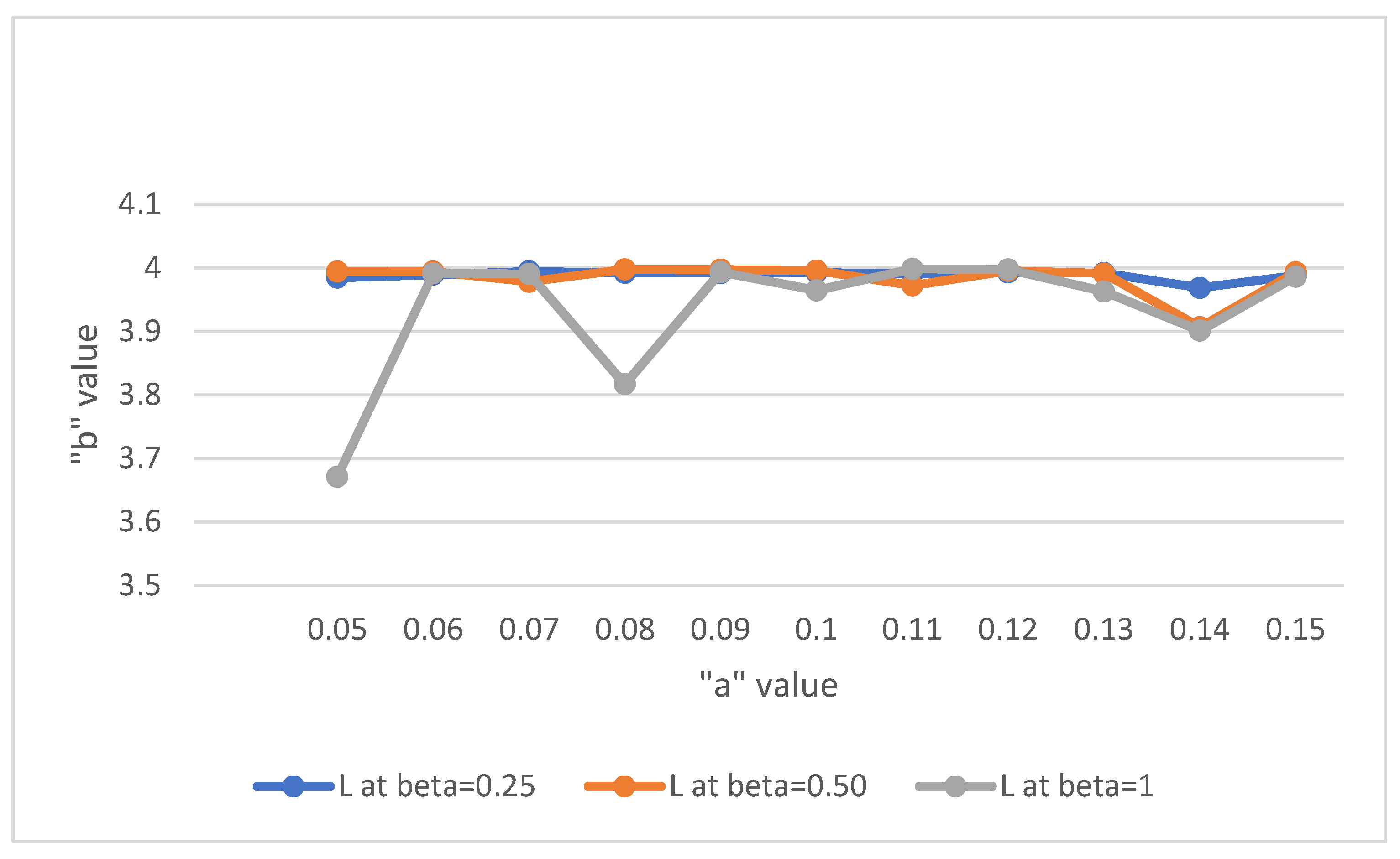
Table 5.
The values of L for different values of b = 0.25, 0.50, 1.
Table 5.
The values of L for different values of b = 0.25, 0.50, 1.
| a | L at b = 0.25 | L at b = 0.50 | L at b = 1 |
|---|
| 0.05 | 3.984371 | 3.994342 | 3.670805 |
| 0.06 | 3.989045 | 3.994022 | 3.991227 |
| 0.07 | 3.994445 | 3.978169 | 3.990492 |
| 0.08 | 3.991879 | 3.997466 | 3.816650 |
| 0.09 | 3.991760 | 3.997145 | 3.993229 |
| 0.10 | 3.992748 | 3.995779 | 3.964409 |
| 0.11 | 3.990344 | 3.972103 | 3.998272 |
| 0.12 | 3.992591 | 3.995301 | 3.997578 |
| 0.13 | 3.992015 | 3.991104 | 3.962625 |
| 0.14 | 3.968499 | 3.906548 | 3.901016 |
| 0.15 | 3.988080 | 3.992987 | 3.985997 |
Table 6.
Comparison of L-Expected number of units in the system between poisson and encouraged arrival.
Table 6.
Comparison of L-Expected number of units in the system between poisson and encouraged arrival.
| a | Poisson Arrival
L at b = 0.50 | Encouraged Arrival
L at b = 0.50 |
|---|
| 0.14 | 3.924853 | 3.906548 |
Table 7.
Comparison of L-Expected number of units in the system between poisson and encouraged arrival.
Table 7.
Comparison of L-Expected number of units in the system between poisson and encouraged arrival.
| a | Poisson Arrival
L at b = 1 | Encouraged Arrival
L at b = 1 |
|---|
| 0.05 | 3.991214 | 3.670805 |
| 0.08 | 3.985968 | 3.816650 |
| 0.10 | 3.982482 | 3.964409 |
| 0.13 | 3.977268 | 3.962625 |
| 0.14 | 3.975535 | 3.901016 |
Table 8.
Verification of Little’s law.
Table 8.
Verification of Little’s law.
| S.No | b | a | L | W | L/W | λ |
|---|
| 1 | 0.25 | 0.05 | 3.984371 | 0.62255797 | 6.399999679 | 6.4 |
| 2 | 0.5 | 0.05 | 3.994342 | 0.62411594 | 6.399999359 | 6.4 |
| 3 | 1 | 0.05 | 3.670805 | 0.57356328 | 6.400003138 | 6.4 |
| 4 | 0.25 | 0.06 | 3.989045 | 0.62328828 | 6.400002888 | 6.4 |
| 5 | 0.5 | 0.06 | 3.994022 | 0.62406594 | 6.399999359 | 6.4 |
| 6 | 1 | 0.06 | 3.990492 | 0.62351438 | 6.400003849 | 6.4 |
| 7 | 0.25 | 0.07 | 3.994445 | 0.62413203 | 6.400008332 | 6.4 |
| 8 | 0.5 | 0.07 | 3.978169 | 0.62158891 | 6.399999035 | 6.4 |
| 9 | 1 | 0.07 | 3.990492 | 0.62351438 | 6.400003849 | 6.4 |
| 10 | 0.25 | 0.08 | 3.991879 | 0.62373109 | 6.400000962 | 6.4 |
| 11 | 0.5 | 0.08 | 3.997466 | 0.62460406 | 6.40000064 | 6.4 |
| 12 | 1 | 0.08 | 3.816650 | 0.59635156 | 6.399995305 | 6.4 |
| 13 | 0.25 | 0.09 | 3.991760 | 0.62371250 | 6.399994869 | 6.4 |
| 14 | 0.5 | 0.09 | 3.997145 | 0.62455391 | 6.399999039 | 6.4 |
| 15 | 1 | 0.09 | 3.993229 | 0.62394203 | 6.400000321 | 6.4 |
| 16 | 0.25 | 0.1 | 3.992748 | 0.62386688 | 6.399998718 | 6.4 |
| 17 | 0.5 | 0.1 | 3.995779 | 0.62434047 | 6.400004805 | 6.4 |
| 18 | 1 | 0.1 | 3.964409 | 0.61943891 | 6.399999031 | 6.4 |
| 19 | 0.25 | 0.11 | 3.990344 | 0.62349125 | 6.400002566 | 6.4 |
| 20 | 0.5 | 0.11 | 3.972103 | 0.62064109 | 6.400000967 | 6.4 |
| 21 | 1 | 0.11 | 3.998272 | 0.62473000 | 6.4 | 6.4 |
| 22 | 0.25 | 0.12 | 3.992591 | 0.62384234 | 6.400003527 | 6.4 |
| 23 | 0.5 | 0.12 | 3.995301 | 0.62426578 | 6.399997757 | 6.4 |
| 24 | 1 | 0.12 | 3.997578 | 0.62466844 | 6.399524227 | 6.4 |
| 25 | 0.25 | 0.13 | 3.992015 | 0.62375234 | 6.400003527 | 6.4 |
| 26 | 0.5 | 0.13 | 3.991104 | 0.62361000 | 6.4 | 6.4 |
| 27 | 1 | 0.13 | 3.962625 | 0.61916016 | 6.400001615 | 6.4 |
| 28 | 0.25 | 0.14 | 3.968499 | 0.62007797 | 6.399999677 | 6.4 |
| 29 | 0.5 | 0.14 | 3.906548 | 0.61039813 | 6.400001311 | 6.4 |
| 30 | 1 | 0.14 | 3.901016 | 0.60953375 | 6.399997375 | 6.4 |
| 31 | 0.25 | 0.15 | 3.988080 | 0.6231375 | 6.399994865 | 6.4 |
| 32 | 0.5 | 0.15 | 3.992987 | 0.62390422 | 6.400002244 | 6.4 |
| 33 | 1 | 0.15 | 3.985997 | 0.62281203 | 6.400000321 | 6.4 |
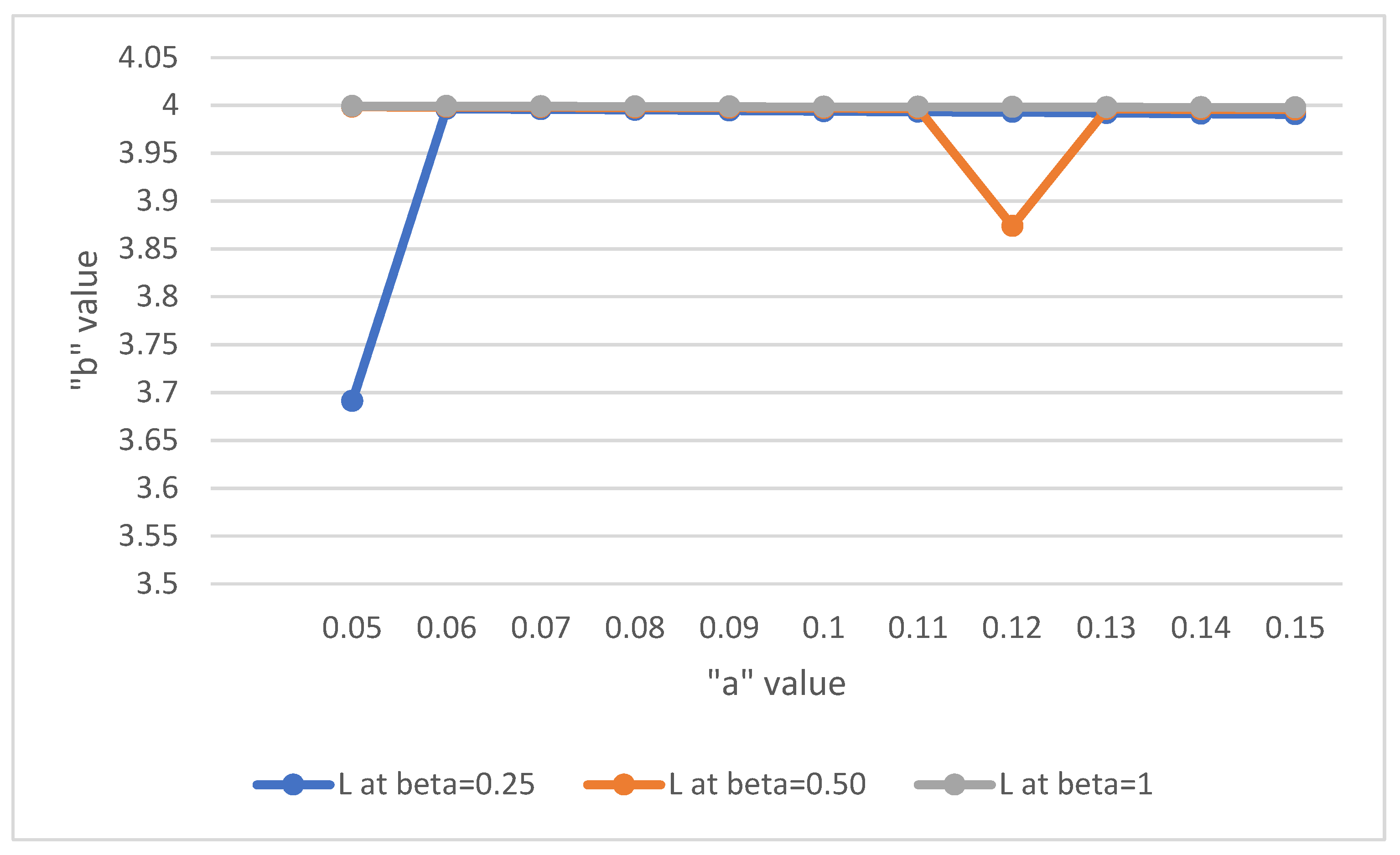
Table 9.
The values of L for different values of b = 0.25, 0.50, 1.
Table 9.
The values of L for different values of b = 0.25, 0.50, 1.
| a | L at b = 0.25 | L at b = 0.50 | L at b = 1 |
|---|
| 0.05 | 3.691028 | 3.998519 | 3.999239 |
| 0.06 | 3.996364 | 3.998222 | 3.999115 |
| 0.07 | 3.995741 | 3.997918 | 3.998966 |
| 0.08 | 3.995176 | 3.997620 | 3.998820 |
| 0.09 | 3.994538 | 3.997342 | 3.998671 |
| 0.10 | 3.993821 | 3.997006 | 3.998423 |
| 0.11 | 3.993171 | 3.996615 | 3.998422 |
| 0.12 | 3.992940 | 3.873728 | 3.998231 |
| 0.13 | 3.991847 | 3.996127 | 3.998082 |
| 0.14 | 3.991183 | 3.995767 | 3.997902 |
| 0.15 | 3.990506 | 3.995525 | 3.997780 |
Table 10.
Comparison of L-Expected number of units in the system between poisson and encouraged arrival.
Table 10.
Comparison of L-Expected number of units in the system between poisson and encouraged arrival.
| a | Poisson Arrival
L at b = 0.50 | Encouraged Arrival
L at b = 0.50 |
|---|
| 0.05 | 3.908215 | 3.691028 |
Table 11.
Comparison of L-Expected number of units in the system between poisson and encouraged arrival.
Table 11.
Comparison of L-Expected number of units in the system between poisson and encouraged arrival.
| a | Poisson Arrival
L at b = 1 | Encouraged Arrival
L at b = 1 |
|---|
| 0.12 | 3.935285 | 3.873728 |
Table 12.
Verification of Little’s law.
Table 12.
Verification of Little’s law.
| S.No | B | a | L | W | L/W | λ |
|---|
| 1 | 0.25 | 0.05 | 3.691028 | 0.54279824 | 6.800002948 | 6.8 |
| 2 | 0.5 | 0.05 | 3.998519 | 0.58801750 | 6.799994218 | 6.8 |
| 3 | 1 | 0.05 | 3.999239 | 0.58812338 | 6.800004421 | 6.8 |
| 4 | 0.25 | 0.06 | 3.996364 | 0.58770059 | 6.799995236 | 6.8 |
| 5 | 0.5 | 0.06 | 3.998222 | 0.58797382 | 6.799997959 | 6.8 |
| 6 | 1 | 0.06 | 3.999115 | 0.58810515 | 6.8000017 | 6.8 |
| 7 | 0.25 | 0.07 | 3.995741 | 0.58760897 | 6.79999966 | 6.8 |
| 8 | 0.5 | 0.07 | 3.997918 | 0.58792912 | 6.800001361 | 6.8 |
| 9 | 1 | 0.07 | 3.998966 | 0.58808324 | 6.800002721 | 6.8 |
| 10 | 0.25 | 0.08 | 3.995176 | 0.58752588 | 6.799998638 | 6.8 |
| 11 | 0.5 | 0.08 | 3.997620 | 0.58788529 | 6.800003402 | 6.8 |
| 12 | 1 | 0.08 | 3.998820 | 0.58806176 | 6.799997279 | 6.8 |
| 13 | 0.25 | 0.09 | 3.994538 | 0.58743206 | 6.800000681 | 6.8 |
| 14 | 0.5 | 0.09 | 3.997342 | 0.58784441 | 6.800004763 | 6.8 |
| 15 | 1 | 0.09 | 3.998671 | 0.58803985 | 6.799998299 | 6.8 |
| 16 | 0.25 | 0.1 | 3.993821 | 0.58732662 | 6.799995573 | 6.8 |
| 17 | 0.5 | 0.1 | 3.997006 | 0.58779500 | 6.8 | 6.8 |
| 18 | 1 | 0.1 | 3.998423 | 0.58800338 | 6.800004422 | 6.8 |
| 19 | 0.25 | 0.11 | 3.993171 | 0.58723103 | 6.800000341 | 6.8 |
| 20 | 0.5 | 0.11 | 3.996615 | 0.58773750 | 6.799994215 | 6.8 |
| 21 | 1 | 0.11 | 3.998422 | 0.58800324 | 6.800002721 | 6.8 |
| 22 | 0.25 | 0.12 | 3.992940 | 0.58719706 | 6.800000681 | 6.8 |
| 23 | 0.5 | 0.12 | 3.873728 | 0.56966588 | 6.799998596 | 6.8 |
| 24 | 1 | 0.12 | 3.998231 | 0.58797515 | 6.800001701 | 6.8 |
| 25 | 0.25 | 0.13 | 3.991847 | 0.58703632 | 6.800003748 | 6.8 |
| 26 | 0.5 | 0.13 | 3.996127 | 0.58766574 | 6.799996937 | 6.8 |
| 27 | 1 | 0.13 | 3.998082 | 0.58795324 | 6.800002721 | 6.8 |
| 28 | 0.25 | 0.14 | 3.991183 | 0.58693868 | 6.799996252 | 6.8 |
| 29 | 0.5 | 0.14 | 3.995767 | 0.58761279 | 6.799997617 | 6.8 |
| 30 | 1 | 0.14 | 3.997902 | 0.58792676 | 6.799997279 | 6.8 |
| 31 | 0.25 | 0.15 | 3.990506 | 0.58683912 | 6.800001363 | 6.8 |
| 32 | 0.5 | 0.15 | 3.995525 | 0.58757721 | 6.800002383 | 6.8 |
| 33 | 1 | 0.15 | 3.997780 | 0.58790882 | 6.799997959 | 6.8 |
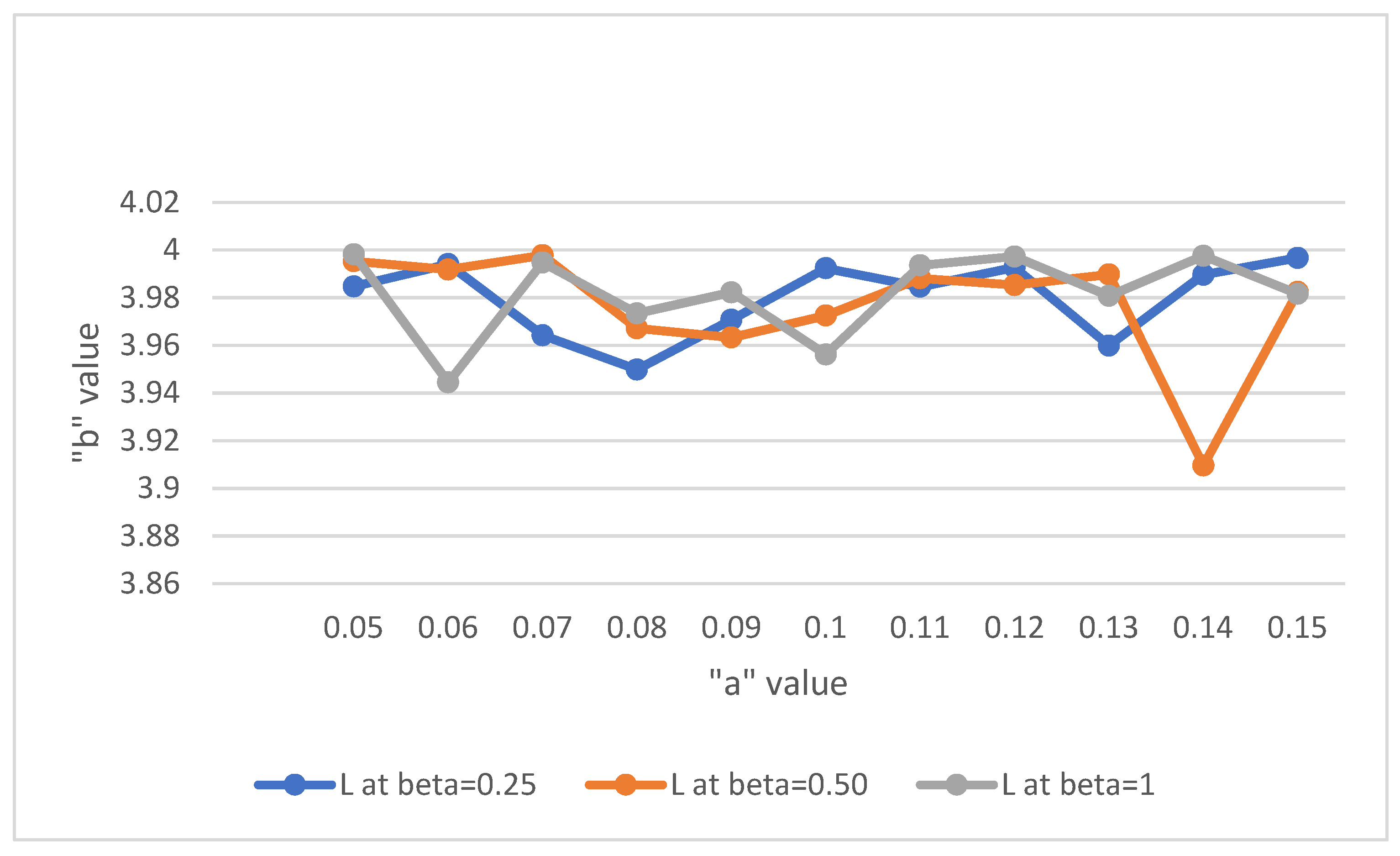
Table 13.
The values of L for different values of b = 0.25, 0.50, 1.
Table 13.
The values of L for different values of b = 0.25, 0.50, 1.
| a | L at b = 0.25 | L at b = 0.50 | L at b = 1 |
|---|
| 0.05 | 3.984716 | 3.995301 | 3.998185 |
| 0.06 | 3.994041 | 3.991779 | 3.944412 |
| 0.07 | 3.964199 | 3.997761 | 3.994704 |
| 0.08 | 3.949832 | 3.967141 | 3.973384 |
| 0.09 | 3.970734 | 3.963279 | 3.982187 |
| 0.10 | 3.992297 | 3.972509 | 3.956158 |
| 0.11 | 3.984562 | 3.988086 | 3.993573 |
| 0.12 | 3.992639 | 3.985290 | 3.997242 |
| 0.13 | 3.959906 | 3.989724 | 3.980712 |
| 0.14 | 3.989582 | 3.909560 | 3.997553 |
| 0.15 | 3.996673 | 3.982409 | 3.981590 |
Table 14.
Comparison of L-Expected number of units in the system between poisson and encouraged arrival.
Table 14.
Comparison of L-Expected number of units in the system between poisson and encouraged arrival.
| a | Poisson Arrival
L at b = 0.50 | Encouraged Arrival
L at b = 0.50 |
|---|
| 0.14 | 3.924853 | 3.909560 |
Table 15.
Comparison of L-Expected number of units in the system between poisson and encouraged arrival.
Table 15.
Comparison of L-Expected number of units in the system between poisson and encouraged arrival.
| a | Poisson Arrival
L at b = 1 | Encouraged Arrival
L at b = 1 |
|---|
| 0.06 | 3.989463 | 3.944412 |
| 0.08 | 3.985968 | 3.973384 |
| 0.09 | 3.984224 | 3.982187 |
| 0.10 | 3.982482 | 3.956158 |
Table 16.
Verification of Little’s law.
Table 16.
Verification of Little’s law.
| S.No | b | a | L | W | L/W | λ |
|---|
| 1 | 0.25 | 0.05 | 3.984716 | 0.55343278 | 7.199997109 | 7.2 |
| 2 | 0.5 | 0.05 | 3.995301 | 0.55490292 | 7.199998919 | 7.2 |
| 3 | 1 | 0.05 | 3.998185 | 0.55530347 | 7.200006123 | 7.2 |
| 4 | 0.25 | 0.06 | 3.994041 | 0.55472792 | 7.199998918 | 7.2 |
| 5 | 0.5 | 0.06 | 3.991779 | 0.55441375 | 7.199996753 | 7.2 |
| 6 | 1 | 0.06 | 3.944412 | 0.54783500 | 7.2 | 7.2 |
| 7 | 0.25 | 0.07 | 3.964199 | 0.55058319 | 7.200002543 | 7.2 |
| 8 | 0.5 | 0.07 | 3.997761 | 0.55524458 | 7.199994597 | 7.2 |
| 9 | 1 | 0.07 | 3.994704 | 0.55482000 | 7.2 | 7.2 |
| 10 | 0.25 | 0.08 | 3.949832 | 0.54858778 | 7.199997083 | 7.2 |
| 11 | 0.5 | 0.08 | 3.967141 | 0.55099181 | 7.199997459 | 7.2 |
| 12 | 1 | 0.08 | 3.973384 | 0.55185889 | 7.19999855 | 7.2 |
| 13 | 0.25 | 0.09 | 3.970734 | 0.55149083 | 7.199997824 | 7.2 |
| 14 | 0.5 | 0.09 | 3.963279 | 0.55045542 | 7.20000545 | 7.2 |
| 15 | 1 | 0.09 | 3.982187 | 0.55308153 | 7.199993853 | 7.2 |
| 16 | 0.25 | 0.1 | 3.992297 | 0.55448569 | 7.199996032 | 7.2 |
| 17 | 0.5 | 0.1 | 3.972509 | 0.55173736 | 7.200004712 | 7.2 |
| 18 | 1 | 0.1 | 3.956158 | 0.54946639 | 7.200005096 | 7.2 |
| 19 | 0.25 | 0.11 | 3.984562 | 0.55341139 | 7.20000506 | 7.2 |
| 20 | 0.5 | 0.11 | 3.988086 | 0.55390083 | 7.199997834 | 7.2 |
| 21 | 1 | 0.11 | 3.993573 | 0.55466292 | 7.199998918 | 7.2 |
| 22 | 0.25 | 0.12 | 3.992639 | 0.55453319 | 7.200002525 | 7.2 |
| 23 | 0.5 | 0.12 | 3.985290 | 0.55351250 | 7.199993496 | 7.2 |
| 24 | 1 | 0.12 | 3.997242 | 0.55517250 | 7.199993516 | 7.2 |
| 25 | 0.25 | 0.13 | 3.959906 | 0.54998694 | 7.199999273 | 7.2 |
| 26 | 0.5 | 0.13 | 3.989724 | 0.55412833 | 7.200004331 | 7.2 |
| 27 | 1 | 0.13 | 3.980712 | 0.55287667 | 7.199995659 | 7.2 |
| 28 | 0.25 | 0.14 | 3.989582 | 0.55410861 | 7.199994947 | 7.2 |
| 29 | 0.5 | 0.14 | 3.909560 | 0.54299444 | 7.200005893 | 7.2 |
| 30 | 1 | 0.14 | 3.997553 | 0.55521569 | 7.199996038 | 7.2 |
| 31 | 0.25 | 0.15 | 3.996673 | 0.55509347 | 7.200006125 | 7.2 |
| 32 | 0.5 | 0.15 | 3.982409 | 0.55311236 | 7.200004701 | 7.2 |
| 33 | 1 | 0.15 | 3.981590 | 0.55299861 | 7.199994937 | 7.2 |
Table 17.
The values of L for different values of b = 0.25, 0.50, 1.
Table 17.
The values of L for different values of b = 0.25, 0.50, 1.
| a | L at b = 0.25 | L at b = 0.50 | L at b = 1 |
|---|
| 0.05 | 3.80713 | 3.95550 | 3.89270 |
| 0.06 | 3.96457 | 3.80124 | 3.37690 |
| 0.07 | 3.88220 | 3.87680 | 3.71920 |
| 0.08 | 3.71410 | 3.97520 | 3.98390 |
| 0.09 | 3.98960 | 3.93560 | 3.96960 |
| 0.10 | 3.80066 | 3.94490 | 3.63780 |
| 0.11 | 3.83620 | 3.75970 | 3.95590 |
| 0.12 | 3.98890 | 3.94710 | 3.99470 |
| 0.13 | 3.98770 | 3.99320 | 3.97470 |
| 0.14 | 3.98853 | 3.97796 | 3.98021 |
| 0.15 | 3.96290 | 3.69889 | 3.97548 |
Table 18.
Comparison of L-Expected number of units in the system between poisson and encouraged arrival.
Table 18.
Comparison of L-Expected number of units in the system between poisson and encouraged arrival.
| a | Poisson Arrival
L at b = 0.25 | Encouraged Arrival
L at b = 0.25 |
|---|
| 0.05 | 3.908215 | 3.80713 |
| 0.08 | 3.856900 | 3.71410 |
| 0.10 | 3.824116 | 3.80066 |
Table 19.
Comparison of L-Expected number of units in the system between poisson and encouraged arrival.
Table 19.
Comparison of L-Expected number of units in the system between poisson and encouraged arrival.
| a | Poisson Arrival
L at b = 0.50 | Encouraged Arrival
L at b = 0.50 |
|---|
| 0.05 | 3.972583 | 3.95550 |
| 0.06 | 3.967179 | 3.80124 |
| 0.07 | 3.961800 | 3.87680 |
| 0.09 | 3.951119 | 3.93560 |
| 0.10 | 3.945816 | 3.94490 |
| 0.11 | 3.940538 | 3.75970 |
| 0.15 | 3.919673 | 3.69889 |
Table 20.
Comparison of L-Expected number of units in the system between poisson and encouraged arrival.
Table 20.
Comparison of L-Expected number of units in the system between poisson and encouraged arrival.
| a | Poisson Arrival
L at b = 1 | Encouraged Arrival
L at b = 1 |
|---|
| 0.05 | 3.9912 | 3.8927 |
| 0.06 | 3.9894 | 3.3769 |
| 0.07 | 3.9877 | 3.7192 |
| 0.08 | 3.9859 | 3.9839 |
| 0.09 | 3.9842 | 3.9696 |
| 0.10 | 3.9824 | 3.6378 |
| 0.11 | 3.9807 | 3.9559 |
| 0.13 | 3.9772 | 3.9747 |
Table 21.
Verification of Little’s law.
Table 21.
Verification of Little’s law.
| S.No | b | a | L | W | L/W | λ |
|---|
| 1 | 0.25 | 0.05 | 3.80713 | 0.50093816 | 7.600002396 | 7.6 |
| 2 | 0.5 | 0.05 | 3.95550 | 0.52046053 | 7.599993083 | 7.6 |
| 3 | 1 | 0.05 | 3.89270 | 0.51219737 | 7.600109334 | 7.6 |
| 4 | 0.25 | 0.06 | 3.96457 | 0.52165395 | 7.599999233 | 7.6 |
| 5 | 0.5 | 0.06 | 3.80124 | 0.50016316 | 7.600002399 | 7.6 |
| 6 | 1 | 0.06 | 3.37690 | 0.44432895 | 7.599999100 | 7.6 |
| 7 | 0.25 | 0.07 | 3.88220 | 0.51081579 | 7.599996868 | 7.6 |
| 8 | 0.5 | 0.07 | 3.87680 | 0.51010526 | 7.600003921 | 7.6 |
| 9 | 1 | 0.07 | 3.71920 | 0.48936842 | 7.600006539 | 7.6 |
| 10 | 0.25 | 0.08 | 3.71410 | 0.48869737 | 7.600005730 | 7.6 |
| 11 | 0.5 | 0.08 | 3.97520 | 0.52305263 | 7.599994647 | 7.6 |
| 12 | 1 | 0.08 | 3.98390 | 0.52419737 | 7.600005342 | 7.6 |
| 13 | 0.25 | 0.09 | 3.98960 | 0.52494737 | 7.600005334 | 7.6 |
| 14 | 0.5 | 0.09 | 3.93560 | 0.51784211 | 7.600001545 | 7.6 |
| 15 | 1 | 0.09 | 3.96960 | 0.52231579 | 7.599996937 | 7.6 |
| 16 | 0.25 | 0.1 | 3.80066 | 0.50008684 | 7.599997600 | 7.6 |
| 17 | 0.5 | 0.1 | 3.94490 | 0.51906579 | 7.599996918 | 7.6 |
| 18 | 1 | 0.1 | 3.63780 | 0.47865789 | 7.599998329 | 7.6 |
| 19 | 0.25 | 0.11 | 3.83620 | 0.50476316 | 7.600002377 | 7.6 |
| 20 | 0.5 | 0.11 | 3.75970 | 0.49469737 | 7.60000566 | 7.6 |
| 21 | 1 | 0.11 | 3.95590 | 0.52051316 | 7.600002305 | 7.6 |
| 22 | 0.25 | 0.12 | 3.98890 | 0.52485526 | 7.600003811 | 7.6 |
| 23 | 0.5 | 0.12 | 3.94710 | 0.51935526 | 7.600003851 | 7.6 |
| 24 | 1 | 0.12 | 3.99470 | 0.52561842 | 7.600006088 | 7.6 |
| 25 | 0.25 | 0.13 | 3.98770 | 0.52469737 | 7.600005336 | 7.6 |
| 26 | 0.5 | 0.13 | 3.99320 | 0.52542105 | 7.600000761 | 7.6 |
| 27 | 1 | 0.13 | 3.97470 | 0.52298684 | 7.599997705 | 7.6 |
| 28 | 0.25 | 0.14 | 3.98853 | 0.52480658 | 7.599993903 | 7.6 |
| 29 | 0.5 | 0.14 | 3.97796 | 0.52341579 | 7.599996943 | 7.6 |
| 30 | 1 | 0.14 | 3.98021 | 0.52371184 | 7.599997709 | 7.6 |
| 31 | 0.25 | 0.15 | 3.96290 | 0.52143526 | 7.600003836 | 7.6 |
| 32 | 0.5 | 0.15 | 3.69889 | 0.48669605 | 7.600000822 | 7.6 |
| 33 | 1 | 0.15 | 3.97548 | 0.52308947 | 7.600006882 | 7.6 |
Table 22.
The values of L for different values of b = 0.25, 0.50, 1.
Table 22.
The values of L for different values of b = 0.25, 0.50, 1.
| a | L at b = 0.25 | L at b = 0.50 | L at b = 1 |
|---|
| 0.05 | 3.995100 | 3.546800 | 3.998800 |
| 0.06 | 3.854856 | 3.939360 | 3.994395 |
| 0.07 | 3.996000 | 3.621280 | 3.993300 |
| 0.08 | 3.991044 | 3.999263 | 3.980034 |
| 0.09 | 3.990490 | 3.934637 | 3.927608 |
| 0.10 | 3.884795 | 3.982260 | 3.957856 |
| 0.11 | 3.987600 | 3.655474 | 3.969599 |
| 0.12 | 3.941250 | 3.991380 | 3.922006 |
| 0.13 | 3.983723 | 3.995832 | 3.757424 |
| 0.14 | 3.983723 | 3.987378 | 3.996665 |
| 0.15 | 3.983001 | 3.992066 | 3.978019 |
Table 23.
Comparison of L-Expected number of units in the system between poisson and encouraged arrival.
Table 23.
Comparison of L-Expected number of units in the system between poisson and encouraged arrival.
| a | Poisson Arrival
L at b = 0.25 | Encouraged Arrival
L at b = 0.25 |
|---|
| 0.06 | 3.890814 | 3.854856 |
Table 24.
Comparison of L-Expected number of units in the system between poisson and encouraged arrival.
Table 24.
Comparison of L-Expected number of units in the system between poisson and encouraged arrival.
| a | Poisson Arrival
L at b = 0.50 | Encouraged Arrival
L at b = 0.50 |
|---|
| 0.05 | 3.97258 | 3.54680 |
| 0.06 | 3.96717 | 3.93936 |
| 0.07 | 3.96180 | 3.62128 |
| 0.09 | 3.95111 | 3.93463 |
| 0.11 | 3.94053 | 3.65547 |
Table 25.
Comparison of L-Expected number of units in the system between poisson and encouraged arrival.
Table 25.
Comparison of L-Expected number of units in the system between poisson and encouraged arrival.
| a | Poisson Arrival
L at b = 1 | Encouraged Arrival
L at b = 1 |
|---|
| 0.08 | 3.98596 | 3.980034 |
| 0.09 | 3.98422 | 3.927608 |
| 0.10 | 3.98248 | 3.957856 |
| 0.11 | 3.98074 | 3.969599 |
| 0.13 | 3.97726 | 3.757424 |
Table 26.
Verification of Little’s law.
Table 26.
Verification of Little’s law.
| S.No | b | a | L | W | L/W | λ |
|---|
| 1 | 0.25 | 0.05 | 3.9951 | 0.8997973 | 4.440001467 | 4.44 |
| 2 | 0.5 | 0.05 | 3.5468 | 0.79882883 | 4.439999049 | 4.44 |
| 3 | 1 | 0.05 | 3.9988 | 0.90063063 | 4.439998179 | 4.44 |
| 4 | 0.25 | 0.06 | 3.854856 | 0.86821081 | 4.439999032 | 4.44 |
| 5 | 0.5 | 0.06 | 3.93936 | 0.88724324 | 4.440001217 | 4.44 |
| 6 | 1 | 0.06 | 3.9943953 | 0.89963858 | 4.439997933 | 4.44 |
| 7 | 0.25 | 0.07 | 3.996 | 0.9 | 4.44 | 4.44 |
| 8 | 0.5 | 0.07 | 3.62128 | 0.8156036 | 4.439997842 | 4.44 |
| 9 | 1 | 0.07 | 3.9933 | 0.89939189 | 4.439999466 | 4.44 |
| 10 | 0.25 | 0.08 | 3.991044 | 0.89888378 | 4.439998932 | 4.44 |
| 11 | 0.5 | 0.08 | 3.999263 | 0.90073491 | 4.439999556 | 4.44 |
| 12 | 1 | 0.08 | 3.980034 | 0.89640405 | 4.440000268 | 4.44 |
| 13 | 0.25 | 0.09 | 3.99049 | 0.89875901 | 4.440000045 | 4.44 |
| 14 | 0.5 | 0.09 | 3.934637 | 0.8861795 | 4.439997517 | 4.44 |
| 15 | 1 | 0.09 | 3.927608 | 0.8845964 | 4.44000199 | 4.44 |
| 16 | 0.25 | 0.1 | 3.884795 | 0.87495383 | 4.439999131 | 4.44 |
| 17 | 0.5 | 0.1 | 3.98226 | 0.89690541 | 4.440002007 | 4.44 |
| 18 | 1 | 0.1 | 3.957856 | 0.89140901 | 4.440000045 | 4.44 |
| 19 | 0.25 | 0.11 | 3.9876 | 0.89810811 | 4.440000534 | 4.44 |
| 20 | 0.5 | 0.11 | 3.655474 | 0.82330495 | 4.439999757 | 4.44 |
| 21 | 1 | 0.11 | 3.969599 | 0.89405383 | 4.43999915 | 4.44 |
| 22 | 0.25 | 0.12 | 3.94125 | 0.88766892 | 4.439999594 | 4.44 |
| 23 | 0.5 | 0.12 | 3.99138 | 0.89895946 | 4.440002269 | 4.44 |
| 24 | 1 | 0.12 | 3.922006 | 0.88333468 | 4.439998415 | 4.44 |
| 25 | 0.25 | 0.13 | 3.983723 | 0.89723491 | 4.439999554 | 4.44 |
| 26 | 0.5 | 0.13 | 3.995832 | 0.89996216 | 4.4400008 | 4.44 |
| 27 | 1 | 0.13 | 3.757424 | 0.84626667 | 4.439998251 | 4.44 |
| 28 | 0.25 | 0.14 | 3.983723 | 0.89723491 | 4.439999554 | 4.44 |
| 29 | 0.5 | 0.14 | 3.987378 | 0.89805811 | 4.440000534 | 4.44 |
| 30 | 1 | 0.14 | 3.996665 | 0.90014977 | 4.439998889 | 4.44 |
| 31 | 0.25 | 0.15 | 3.9830014 | 0.89707239 | 4.440001917 | 4.44 |
| 32 | 0.5 | 0.15 | 3.992066 | 0.89911396 | 4.439999822 | 4.44 |
| 33 | 1 | 0.15 | 3.978019 | 0.89595023 | 4.440001116 | 4.44 |
Table 27.
The values of L for different values of b = 0.25, 0.50, 1.
Table 27.
The values of L for different values of b = 0.25, 0.50, 1.
| a | L at b = 0.25 | L at b = 0.50 | L at b = 1 |
|---|
| 0.05 | 3.995172 | 3.997721 | 3.998884 |
| 0.06 | 3.994119 | 3.997247 | 3.998651 |
| 0.07 | 3.993030 | 3.996783 | 3.995359 |
| 0.08 | 3.991918 | 3.996305 | 3.998160 |
| 0.09 | 3.990777 | 3.995824 | 3.997972 |
| 0.10 | 3.980430 | 3.990005 | 3.955846 |
| 0.11 | 3.988407 | 3.978139 | 3.993533 |
| 0.12 | 3.987155 | 3.977938 | 3.973857 |
| 0.13 | 3.985937 | 3.984462 | 3.981141 |
| 0.14 | 3.984280 | 3.993300 | 3.990031 |
| 0.15 | 3.981860 | 3.991190 | 3.993370 |
Table 28.
Comparison of L-Expected number of units in the system between poisson and encouraged arrival.
Table 28.
Comparison of L-Expected number of units in the system between poisson and encouraged arrival.
| a | Poisson Arrival
L at b = 1 | Encouraged Arrival
L at b = 1 |
|---|
| 0.10 | 3.98248 | 3.955846 |
Table 29.
Verification of Little’s law.
Table 29.
Verification of Little’s law.
| S.No | b | a | L | W | L/W | λ |
|---|
| 1 | 0.25 | 0.05 | 3.995172 | 0.89177946 | 4.480002332 | 4.48 |
| 2 | 0.5 | 0.05 | 3.997721 | 0.89234844 | 4.480002196 | 4.48 |
| 3 | 1 | 0.05 | 3.998884 | 0.89260804 | 4.480000179 | 4.48 |
| 4 | 0.25 | 0.06 | 3.994119 | 0.89154442 | 4.480002109 | 4.48 |
| 5 | 0.5 | 0.06 | 3.997247 | 0.89224263 | 4.479998162 | 4.48 |
| 6 | 1 | 0.06 | 3.998651 | 0.89255603 | 4.480000134 | 4.48 |
| 7 | 0.25 | 0.07 | 3.99303 | 0.89130134 | 4.480001705 | 4.48 |
| 8 | 0.5 | 0.07 | 3.996783 | 0.89213906 | 4.480000314 | 4.48 |
| 9 | 1 | 0.07 | 3.995359 | 0.89182121 | 4.480001032 | 4.48 |
| 10 | 0.25 | 0.08 | 3.991918 | 0.89105313 | 4.480000628 | 4.48 |
| 11 | 0.5 | 0.08 | 3.996305 | 0.89203237 | 4.480001838 | 4.48 |
| 12 | 1 | 0.08 | 3.99816 | 0.89244643 | 4.480002151 | 4.48 |
| 13 | 0.25 | 0.09 | 3.990777 | 0.89079844 | 4.4800022 | 4.48 |
| 14 | 0.5 | 0.09 | 3.995824 | 0.8919317 | 4.47996484 | 4.48 |
| 15 | 1 | 0.09 | 3.997972 | 0.89240446 | 4.480002331 | 4.48 |
| 16 | 0.25 | 0.1 | 3.98043 | 0.88848884 | 4.47999919 | 4.48 |
| 17 | 0.5 | 0.1 | 3.990005 | 0.89062612 | 4.480000584 | 4.48 |
| 18 | 1 | 0.1 | 3.955846 | 0.88300134 | 4.480001721 | 4.48 |
| 19 | 0.25 | 0.11 | 3.988407 | 0.89026942 | 4.480002112 | 4.48 |
| 20 | 0.5 | 0.11 | 3.978139 | 0.88797746 | 4.480002297 | 4.48 |
| 21 | 1 | 0.11 | 3.993533 | 0.89141362 | 4.47999807 | 4.48 |
| 22 | 0.25 | 0.12 | 3.987155 | 0.88998996 | 4.479999775 | 4.48 |
| 23 | 0.5 | 0.12 | 3.977938 | 0.88793259 | 4.479997928 | 4.48 |
| 24 | 1 | 0.12 | 3.973857 | 0.88702165 | 4.479998241 | 4.48 |
| 25 | 0.25 | 0.13 | 3.985937 | 0.88971808 | 4.480000405 | 4.48 |
| 26 | 0.5 | 0.13 | 3.9844625 | 0.88938895 | 4.479999753 | 4.48 |
| 27 | 1 | 0.13 | 3.981141 | 0.88864754 | 4.479997704 | 4.48 |
| 28 | 0.25 | 0.14 | 3.98428 | 0.88934821 | 4.480001079 | 4.48 |
| 29 | 0.5 | 0.14 | 3.9933 | 0.89136161 | 4.479998025 | 4.48 |
| 30 | 1 | 0.14 | 3.990031 | 0.89063192 | 4.479999596 | 4.48 |
| 31 | 0.25 | 0.15 | 3.98186 | 0.88880804 | 4.48000018 | 4.48 |
| 32 | 0.5 | 0.15 | 3.99119 | 0.89089063 | 4.479998114 | 4.48 |
| 33 | 1 | 0.15 | 3.99337 | 0.89137723 | 4.480001167 | 4.48 |


