Estimation of Asymmetric Spatial Autoregressive Dependence on Irregular Lattices

Abstract

In spatial econometrics, we usually assume that the spatial dependence structure is known and that all information about it is contained in a spatial weights matrix $\mathbf{W}$. However, in practice, the structure of $\mathbf{W}$ is unknown a priori and difficult to obtain, especially for asymmetric dependence. In this paper, we propose a data-driven method to obtain $\mathbf{W}$, whether it is symmetric or asymmetric. This is achieved by calculating the area overlap of the adjacent regions/districts with a given shape (a pizza-like shape, in our case). With $\mathbf{W}$ determined in this way, we estimate the potentially asymmetric spatial autoregressive dependence on irregular lattices. We verify our method using Monte Carlo simulations for finite samples and compare it with classical approaches such as Queen’s contiguity matrices and inverse-distance weighting matrices. Finally, our method is applied to model the evolution of sales prices for building land in Brandenburg, Germany. We show that the price evolution and its spatial dependence are mainly driven by the orientation towards Berlin.

1. Introduction

Geospatial analysis is based on Tobler’s first law of geography, which points out that everything is connected to everything else, but that nearby objects dominate (Tobler [1]). Not every process can be described by applying this rule, and there is no precise and unique definition of “nearby”. Therefore, it is often assumed that the dependence structure is known through underlying physical systems (e.g., river flows) or geographical information or network structures (e.g., public transport connections), or assumptions such as symmetry are made. Generally, to model spatial data, one needs to know the $n(n-1)$ potential interactions among the system’s n objects. A major challenge is to obtain these interactions from the n data points in the sample.

There are various attempts to model such spatial dependence. For instance, the spatial covariance could directly be described by a parametric covariance function that has fewer parameters than all possible links. This approach is commonly known as the geostatistical approach (see, e.g., Cressie and Wikle [2]). Alternatively, spatial dependence could be modeled by explicitly including spatially lagged variables. These models are often referred to as spatial econometrics models. Processes in which the objects/regions influence each other can be modeled with spatial autoregressive (SAR) models (LeSage [3], LeSage and Pace [4]). SAR models describe processes in which the observed value of one region influences the observed value in other regions and vice versa. An exemplary question that such models attempt to answer is whether the average salary in one region influences the average salary in adjacent regions, and if so, to what extent. Such interplay among n regions is described by an $n\times n$ spatial weights matrix $\mathbf{W}$.

These autoregressive-type approaches involving the specification of a weights matrix have been widely used in different areas. For instance, in environmental statistics, the effects of weather conditions on fertilizer application were modelled (Billé and Rogna [5]) and environmental expenditure interactions among OECD countries were investigated. In addition, the impact of COVID on financial returns was investigated (Billé and Caporin [6]), and studies of the labour market have employed spatial weight matrices (Billé [7]). Furthermore, in health economics, Donegan et al. [8] used spatial econometrics approaches for modelling community health.

There are different methods for obtaining a suitable $\mathbf{W}$. One is to assume that all regions sharing a common border influence each other. This method is also called the Queen’s contiguity matrix, alluding to the chessboard (LeSage and Pace [4]). If region A and region B share a common border, the Queen’s contiguity matrix is then constructed with $W_{AB}=W_{BA}=1$. Other methods involve geographical distances such as those used in Lin Lawell [9] to model air pollution. They assume that the first-neighbour regions are the regions within 500 km of each other. Another method for constructing $\mathbf{W}$ is to assume that the regions’ influences on each other declines as the distance between them increases. The so-called ‘inverse-distance $\mathbf{W}$’ was used by Boly et al. [10] to model real-estate valuation and by Zhao et al. [11] to describe air pollution in China. The inverse-distance matrix is constructed with $W_{AB}=W_{BA}=1/distance(A,B)$. An advanced method also takes geographical or economical connections into account when constructing $\mathbf{W}$. Krisztin et al. [12] described the worldwide spread of the coronavirus by assuming that countries with a common border influence each other, as well as countries connected by an airline. Other suggested methods for constructing $\mathbf{W}$ include the parametric or semi-parametric estimation method proposed by Pinkse et al. [13], the method of Stakhovych and Bijmolt [14], where $\mathbf{W}$ was selected from a set of possible candidates with a goodness-of-fit criterion, requiring that the true $\mathbf{W}$ is in the set of candidates, and that of Bhattacharjee and Jensen-Butler [15], where $\mathbf{W}$ was selected from an estimated spatial autocovariance matrix under the conditions of symmetry and a finite sample size of n.

Ahrens and Bhattacharjee [16] proposed to estimate $\mathbf{W}$ in two steps with a least absolute shrinkage and selection operator (lasso) approach. An alternative penalized estimation approach was proposed by Lam and Souza [17]. They selected $\mathbf{W}$ from a linear combination of different weights matrices by setting irrelevant components to zero. This linear combination could involve higher-order spatial lags (see, e.g., Cohen and Paul [18]). A method for selecting the best weights matrix from a set of candidates was also proposed by Debarsy and LeSage [19] or by Debarsy and Ertur [20]. Zhang and Yu [21] showed that the true weights matrix can consistently be selected from the set of candidates (if included) using Mallow’s $C_p$ criterion. If the true matrix is not in the set of candidates, the selection is still optimal, and they proposed a model averaging technique over different candidates. In addition, the method was illustrated by an analysis of historical rice prices in China.

Most of the studies have in common the fact that they apply symmetric weighting schemes (if A influences B, then B influences A, but with a potentially different magnitude). To the best of our knowledge, there are only a few references that deal with the construction of weights matrices accounting for asymmetry. Exceptions include, for instance, Zhou et al. [22], who constructed their asymmetric weights matrix by element-wise multiplication of a nearest-neighbour weights matrix (mostly symmetric) with a matrix that indicated whether the influence flowed from A to B or vice versa. The direction of the influence must be known in advance. A similar method for constructing an asymmetric weights matrix was proposed by Merk and Otto [23], to model ${\mathrm{PM}}_{2.5}$ concentrations. In their approach, the directional component depended on the wind direction and wind speed, which strongly influenced the spatial dependence structure.

However, in practice, we often do not have prior knowledge about the asymmetrical or directional influences. Therefore, in this paper, we develop a data-driven method to estimate the interactions directly from the sample data and explicitly allow asymmetric dependence for irregular lattice data. We assume that the interactions are not dependent on the location of the region but are equal over the entire sample area. With this approach for irregular lattice data, we extend the work of Merk and Otto [24], who proposed a similar approach for obtaining the interactions for regular lattice data based on a lasso procedure. The proposed method respects the interactions from close neighbours, like the Queen’s contiguity matrix or the inverse-distance matrix, but allows asymmetric interactions (if A influences B, B does not necessarily influence A). It is worth noting that the proposed method provides a method of obtaining a flexible weights matrix. This weights matrix can be an additional candidate for the selection of the weights matrix described above, for which good candidates must be available.

This paper is structured as follows. Section 2 describes the theoretical model. Section 3 covers a Monte Carlo simulation study. In Section 4, we apply our method to real-world data and analyse the evolution of land sale prices in Brandenburg, Germany, to show that the short-distance directional influences are coming from Berlin. We conclude by discussing new research directions in Section 5.

2. Theoretical Model

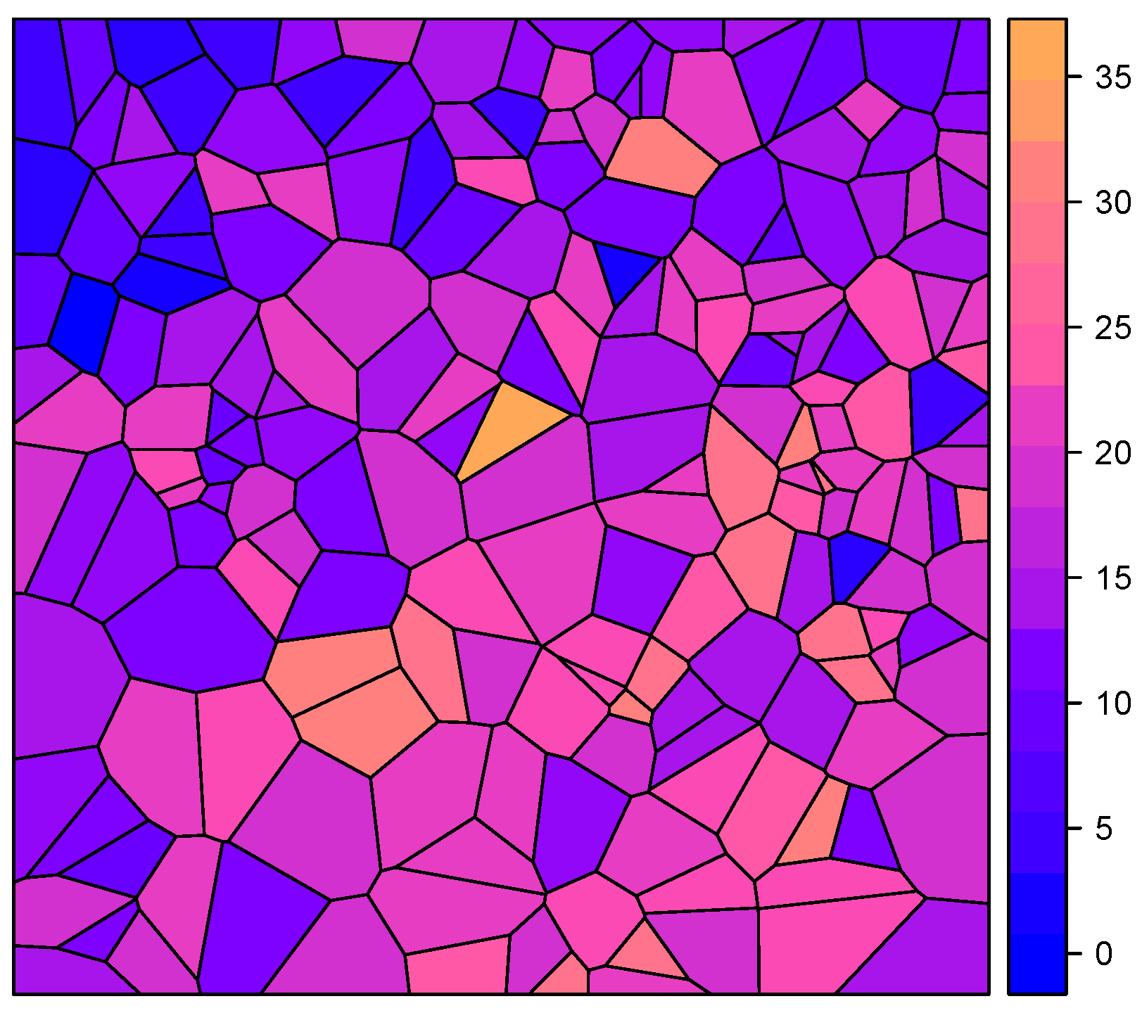
Let $\left\{Y\right(\mathbf{s})\in \mathbb{R}:\mathbf{s}\in B\}$ be a univariate process in the spatial domain B. We explicitly consider B to be an irregular lattice, as would be the case for spatial polygon data. Shapes like this can be found in countries, states, and districts. An artificial example can be seen in Figure 1.

Furthermore, suppose that the process is observed for a finite set of locations $B=\{{\mathbf{s}}_1,\cdots ,{\mathbf{s}}_n\}$ and $\mathit{Y}={(Y\left({\mathbf{s}}_1\right),\cdots ,Y\left({\mathbf{s}}_n\right))}^t$. We consider that the process follows a spatial autoregressive model, i.e.,

$$\mathit{Y}=\mathbf{W}\mathit{Y}+\mathbf{X}\mathbf{\beta }+\mathbf{ϵ},$$

(1)

where $\mathbf{W}$ is an unknown spatial weights matrix and $\mathbf{\beta }$ is a vector of p exogenous influences. Furthermore, $\mathbf{X}$ is a $(p+1)\times n$ matrix and $\mathbf{ϵ}$ is a random error vector, which is assumed to have zero mean with a diagonal, homoscedastic covariance matrix ${\sigma }_{\mathbf{ϵ}}^2\mathbf{I}$. The identity matrix is denoted by $\mathbf{I}$. Since $\mathbf{W}$ consists of $n(n-1)$ unknown parameters, which must be estimated, and only n values of the response are observed, $\mathbf{W}$ is typically replaced by a multiple of a pre-specified matrix $\tilde{\mathbf{W}}$, i.e., $\mathbf{W}=\varphi \tilde{\mathbf{W}}$, where $\varphi$ is an unknown scalar parameter to be estimated (Anselin [25]).

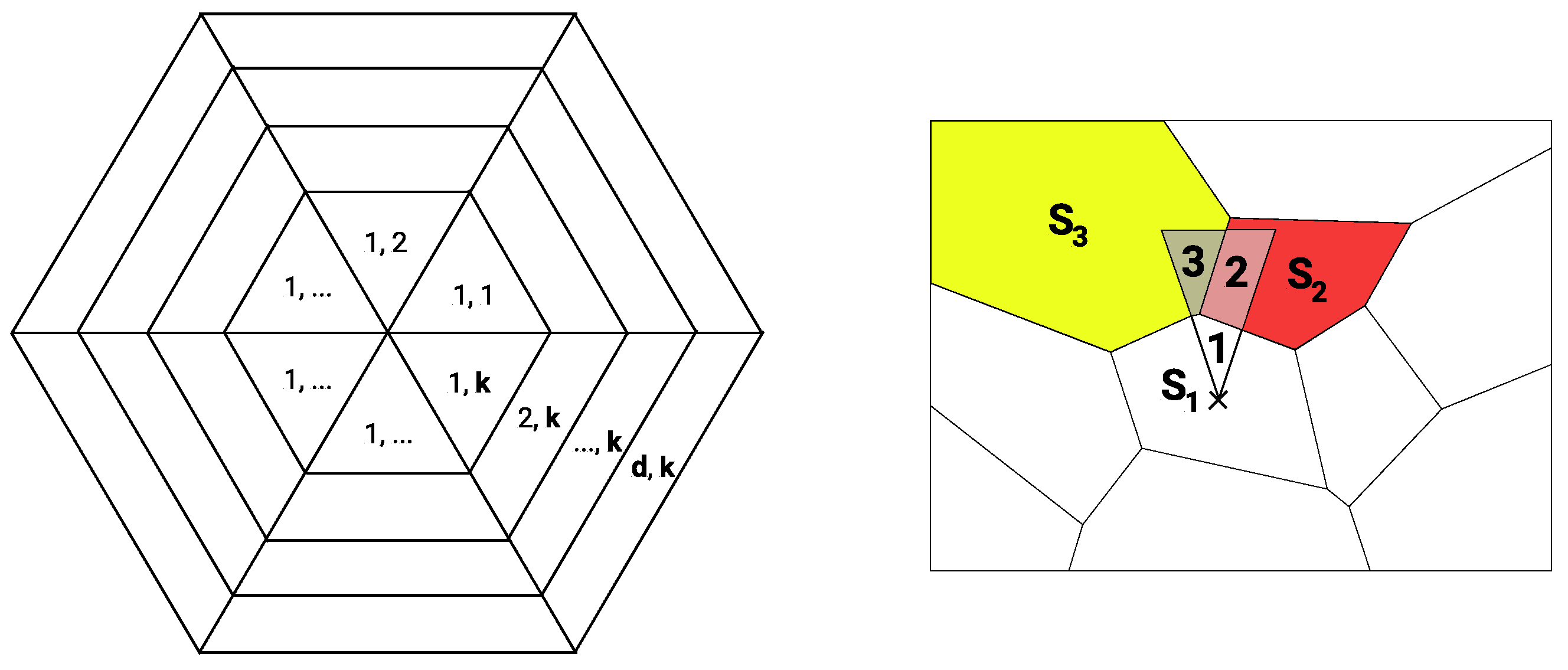
In the following, we aim to estimate the full spatial dependence structure $\mathbf{W}$. To obtain a meaningful and easy-to-interpret representation, suppose that the spatial dependence can be separated into k directions and d distances (see Figure 2a). Furthermore, suppose that there is a unique weighting for each segment of the sectors such that $\mathbf{W}$ can be decomposed as

$$\mathbf{W}=\sum _{i=1}^k\sum _{j=1}^d{\varphi }_{ij}{\tilde{\mathbf{W}}}_{ij},$$

(2)

where each matrix ${\tilde{\mathbf{W}}}_{ij}$ has positive weights for the $\left(ij\right)$th segment only (see Figure 2b). The weights are chosen to be proportional to the overlapping areas. That is,

$${\tilde{\mathbf{W}}}_{ij}=\left(\begin{array}{cccc}0& w_{ij,12}& \cdots & w_{ij,1n}\\ w_{ij,21}& 0& \cdots & w_{ij,2n}\\ ⋮& ⋮& \ddots & ⋮\\ w_{ij,n1}& w_{ij,n2}& \cdots & 0\end{array}\right)={\left(w_{ij,\iota \eta }\right)}_{\iota ,\eta =1,\cdots ,n}$$

(3)

where $w_{ij,\iota \eta }$ is the relative area of the $\eta$th location lying in the $\left(ij\right)$th segment with respect to region $\iota$. For example, (see Figure 2b), one $w_{ij,\iota \eta }$ is the normalized area of 2. Due to normalization, each ${\tilde{\mathbf{W}}}_{ij}$ is bounded by 1 in the row sums. Each of these matrices contains the relative overlapping areas of one segment with the n regions. Since a segment usually overlaps with a small fraction of the regions only, all ${\tilde{\mathbf{W}}}_{ij}$ are sparse.

Figure 2b depicts an artificial map of ten regions. An exemplary segment $\left({\varphi }_{ij}\right)$ determines the spatial dependence of the region $S_1$ towards the north by the relative sizes of its overlap with the neighbouring regions $S_2$ and $S_3$. As we exclude self-influences, the overlap with region $S_1$ is ignored, and the weights for the spatial dependence are normalized with respect to the two remaining intersections. Here, the weights are given by $w_{ij,12}=0.6$ and $w_{ij,13}=0.4$ for $S_2$ and $S_3$, respectively. With this construction, the matrix $\left(w_{ij,\iota \eta }\right)$ is row-normalized, as $w_{ij,12}$ and $w_{ij,13}$ are the only non-zero entries in row $\iota =1$.

This leads to the classical autoregressive model with higher-order spatial lags, given by

$$\mathit{Y}=\sum _{i=1}^k\sum _{j=1}^d{\varphi }_{ij}{\tilde{\mathbf{W}}}_{ij}\mathit{Y}+\mathbf{X}\mathbf{\beta }+\mathbf{ϵ}.$$

(4)

In the reduced form, we obtain with

$$\mathbf{S}\{{\varphi }_{ij}:i=1,\cdots ,k;j=1,\cdots ,d\}=\mathbf{I}-\sum _{i=1}^k\sum _{j=1}^d{\varphi }_{ij}{\tilde{\mathbf{W}}}_{ij}$$

(5)

that

$$\mathit{Y}={\left(\mathbf{I}-\sum _{i=1}^k\sum _{j=1}^d{\varphi }_{ij}{\tilde{\mathbf{W}}}_{ij}\right)}^{-1}(\mathbf{X}\mathbf{\beta }+\mathbf{ϵ})=\mathbf{S}{\left\{{\varphi }_{ij}\right\}}^{-1}(\mathbf{X}\mathbf{\beta }+\mathbf{ϵ}).$$

(6)

In this paper, we consider that d and k are chosen to be large enough to obtain a flexible model reflecting the true underlying spatial dependence precisely, generally leading to a rich, parameterized description.

The inverse ${\mathbf{S}}^{-1}$ exists if the column-sum norm ${\Vert \mathbf{W}\Vert }_1<a$ or the row-sum norm ${\Vert \mathbf{W}\Vert }_{\infty }<a$ is bounded by a finite number a. With the ${\tilde{\mathbf{W}}}_{ij}$ row sums bounded by 1, this can be ensured under the assumption that

$$\sum _{i=1}^k\sum _{j=1}^d\left|{\varphi }_{ij}\right|<1.$$

(7)

A more general condition is discussed by Elhorst et al. [26]. Since we only want to describe the direction from which we see a stronger or weaker influence, we constrain ourselves to the first condition.

Implementing the model demands a proper choice of the parameters k and d, which determine the division of the direction and distance of the spatial dependence, respectively. Moreover, the actual length of each distance step can be optimally chosen. We perform a spatial partitioning analysis to obtain a robust choice of all three parameters.

Let $l_q$ be the distance between the qth and $(q+1)$th distance steps. We suggest selecting $k\in K\subset \mathbb{N}$, $d\in D\subset \mathbb{N}$, and $l_q\in L\subset {\mathbb{R}}_{>0}$ using Akaike information criterion (AIC) selection (Akaike [27]). Therefore, we calculate all ${\tilde{\mathbf{W}}}_{ij}(k,d,l_q)$ for different sets of $D\times K\times L$. Then, we estimate the unknown parameters $\mathbf{\beta },{\varphi }_{ij}$ with maximum-likelihood methods and select the best-performing model based on its AIC. Having obtained the best-fitting $(\widehat{k},\widehat{d},{\widehat{l}}_q)$, we estimate the final model in the next step.

We estimate the parameters $\{\mathbf{\beta },{\varphi }_{ij}\}$ using the maximum-likelihood approach combined with parameter selection using minimal AIC. For both symmetric and asymmetric dependence, a large share of the ${\varphi }_{ij}$ values can be expected to be zero, because k and d are large. For this reason, we repeat the estimation $d\times k$ times and, at every step, we drop the least significant ${\varphi }_{ij}$ parameter (i.e., we set this particular ${\varphi }_{ij}$ to zero). Finally, from these $d\times k$ estimations we choose the one with the lowest AIC.

In general, the unknown parameters $\{\mathbf{\beta },{\varphi }_{ij}\}$ can be estimated. For that reason, the joint probability function, the log-likelihood function $f_{\mathit{Y}}\left(\mathit{Y}\right)$, is maximized with respect to parameters ${\varphi }_{ij}$ and $\mathbf{\beta }$. Assuming that $\mathbf{ϵ}\sim N(\mathbf{0},{\sigma }_{\mathbf{ϵ}}^2\mathbf{I})$, the log-likelihood is given by

$$\mathcal{L}\left(\mathit{Y}\right|\mathbf{\beta },{\varphi }_{ij})=\frac{n}{2}log\left(2\pi {\sigma }_{\mathbf{ϵ}}^2\right)-\frac{1}{2{\sigma }_{\mathbf{ϵ}}^2}{\widetilde{\mathbf{ϵ}}}^t\widetilde{\mathbf{ϵ}}+logdet\left(\mathbf{S}\right)$$

(8)

with

$$\widetilde{\mathbf{ϵ}}=\left(\mathbf{I}-\sum _{i=1}^k\sum _{j=1}^d{\varphi }_{ij}{\tilde{\mathbf{W}}}_{ij}\right)\mathit{Y}-\mathbf{X}\mathbf{\beta }=\mathbf{S}\mathit{Y}-\mathbf{X}\mathbf{\beta }.$$

(9)

The estimator is obtained by maximizing Equation (8) with respect to all parameters. For the consistency of the resulting estimators, we refer to Lee [28] and Gupta and Robinson [29].

3. Monte Carlo Simulations

For the simulation study, we simulate the irregular spatial lattice as Voronoi cells (Longley et al. [30], Sen [31]), where $n\in \{200,500,900\}$ centroids are sampled from a two-dimensional uniform distribution on the interval ${[0,\sqrt{n}]}^2$ (see Figure 1). Eventually, $\mathit{Y}$ can be simulated as in Equation (6), with $\mathbf{ϵ}$ being uncorrelated realizations of a standard normal distribution. We choose $\mathbf{\beta }={(3,1,2,0,5)}^t$ and $\mathbf{X}$ has only ones in the first column. The remaining elements are standard normally distributed random values.

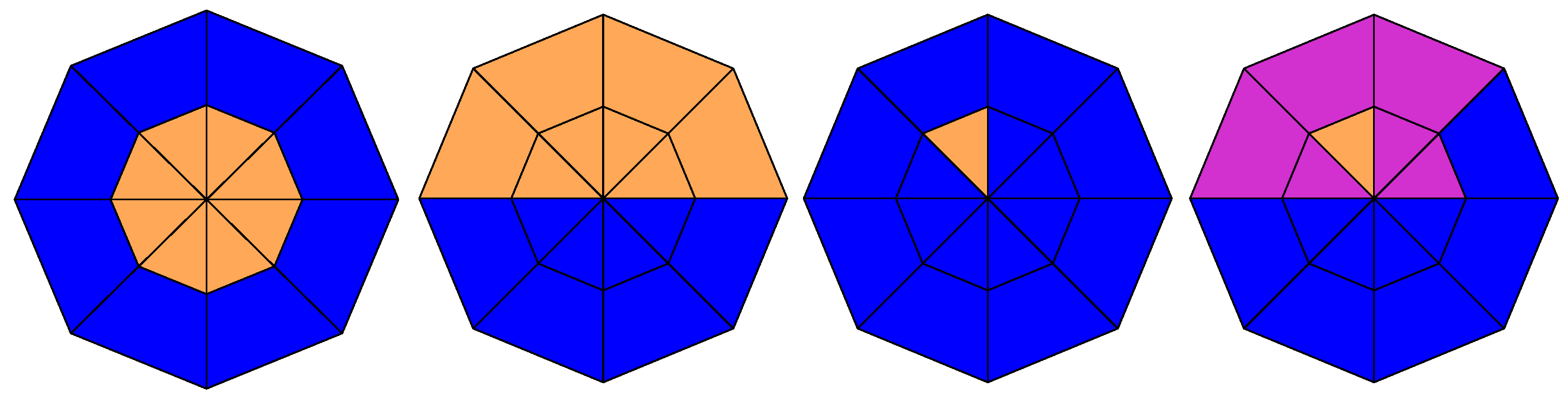
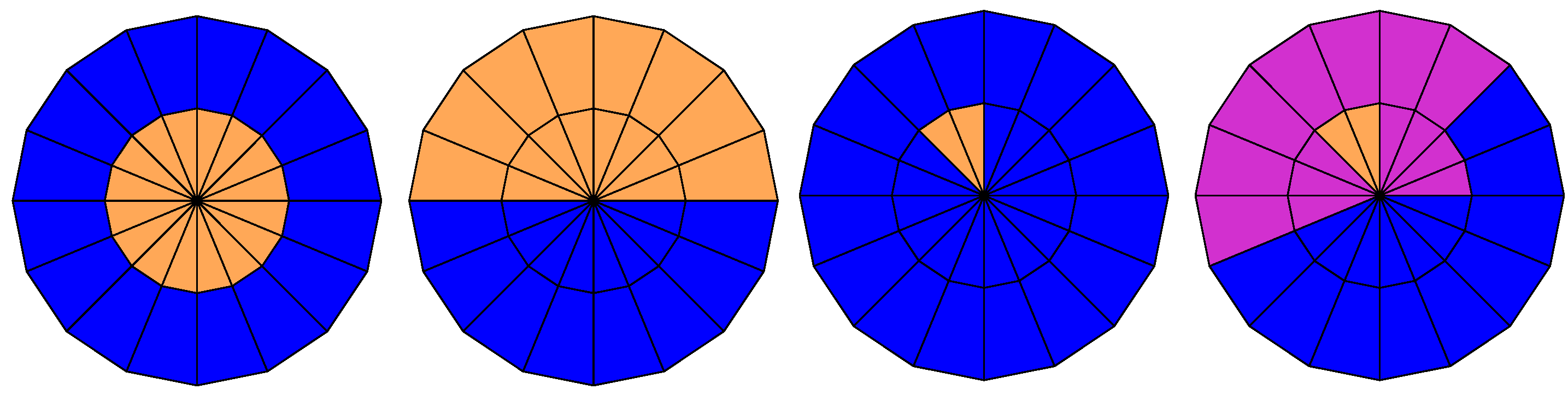
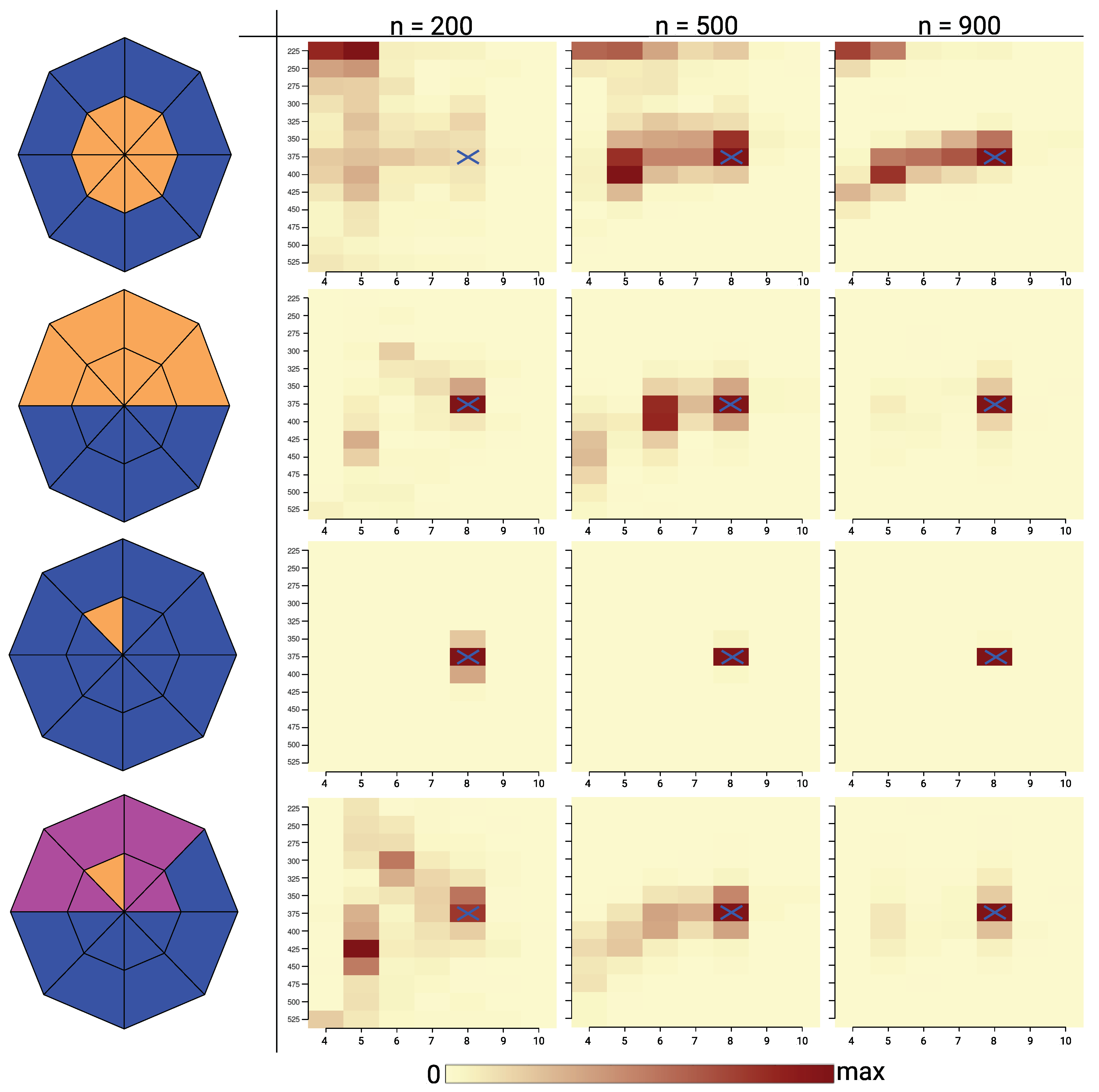
We consider four different specifications of the spatial dependence with $k=8$ and $k=16$, as shown in Figure 3 and Figure 4. First, an isotropic process is considered where only the first lag has an influence, as in classical contiguity settings. Second, a directional process is considered with a clear north-to-south dependence. Third, we consider a nearest-neighbour dependence in the northwest direction only. Finally, the fourth setting is extended by adding another level of dependence strength, while retaining the mainly northwest directional dependence. Blue sections represent zero influence, orange sections represent the maximum influence, and purple sections represent $50\%$ of the maximum influence. The maximum influence is obtained by setting ${\sum }_{i=1}^k{\sum }_{j=1}^d\left|{\varphi }_{ij}\right|=0.95$.

We carried out two types of simulation. In the first type, we used $d=2$, $k=8$ and $l=375$, employing the spatial dependence structures depicted in Figure 3. We first performed the spatial partitioning (results in

Table 1. Means and standard deviations of the best $\tilde{k}$ and $\tilde{l}$ for ${10}^3$ estimations. For each setting, the best values are printed in bold. The greater the value of n, the closer we approach to the true values of $k=8$ and $l=375$.

	8-Setting-1			8-Setting-2			8-Setting-3			8-Setting-4
n	200	500	900	200	500	900	200	500	900	200	500	900
mean($\tilde{k}$)	5.34	6.17	6.29	6.8	6.43	7.51	7.99	8	8	6.26	6.59	7.36
sd($\tilde{k}$)	1.31	1.39	1.35	1.37	1.44	1.07	0.16	0	0	1.31	1.47	1.22
mean($\tilde{l}$)	325	336	347	382	393	376	377	375	374	379	389	375
sd($\tilde{l}$)	86	65	66	58	37	30	18	7.1	4.5	69	36	37

and Figure 5) to gain the best $\tilde{k}$ and $\tilde{l}$ for the estimation of ${\widehat{\varphi }}_{ij}$ (we use $\tilde{k}$ to denote the optimal parameter and $\widehat{k}$ to denote an estimator). The procedure to determine $\tilde{k}$ and $\tilde{l}$ is described below, and was repeated ${10}^3$ times. Then, using the optimal ($\tilde{k},\tilde{l}$) from each of the 1000 estimations, we estimated ${\widehat{\varphi }}_{ij}$ and compared it to alternative estimations with the Queen’s contiguity matrix, the inverse-distance neighbour matrix by AIC, and the sum of squared residuals (${ϵ}^2$). The comparison can be found in

Table 2. One thousand estimations of $\widehat{\mathbf{y}}$ using this method. The results are compared, using the average AIC and ${\mathbf{ϵ}}^2$, to estimations with Queen’s contiguity matrices and inverse-distance weighting matrices. The values of $\tilde{k}$ and $\tilde{l}$ are chosen from spatial partitioning.

		8-Setting-1			8-Setting-2			8-Setting-3			8-Setting-4
	n	200	500	900	200	500	900	200	500	900	200	500	900
AIC	Our Method	570	1431	2573	568	1426	2562	573	1439	2592	568	1425	2563
	Queen	671	1541	2846	654	1569	2965	785	2015	3438	644	1612	2901
	Inv. Dist.	652	1539	2859	652	1552	2868	775	2031	3445	636	1597	2815
${\mathbf{ϵ}}^2$	Our Method	0.954	0.987	1.000	0.947	0.984	0.995	1.016	1.035	1.040	0.957	0.986	0.996
	Queen	1.343	1.245	1.341	1.299	1.370	1.497	2.561	2.942	2.507	1.314	1.370	1.381
	Inv. Dist.	1.201	1.225	1.337	1.256	1.293	1.321	2.377	3.111	2.515	1.229	1.314	1.268

, showing that our method works best.

In the second type of simulation, we show that we can re-estimate even higher-dimensional specifications of the spatial dependence, as depicted in Figure 4. We simulated $\mathit{Y}$ with $d=2$, $k=16$ and $l_1=l_2=375$ using this high-resolution spatial dependence and estimated ${\widehat{\varphi }}_{ij}$, conditionally upon selecting the true d, k and l as the best parameters. The results are summarized in

Table 3. Mean of 500 estimates for each of the 4 different settings with 3 different values of n. We compare the BIAS, RMSE, true positive selections, and false negative selections. The values for BIAS and RMSE are to the power of ${10}^{-3}$ and are separated between values that should be estimated as zero ($\stackrel{!}{=}0$) and values that should be estimated as greater than zero ($\stackrel{!}{>}0$).

		16-Setting-1			16-Setting-2			16-Setting-3			16-Setting-4
	n	200	500	900	200	500	900	200	500	900	200	500	900
BIAS	$\stackrel{!}{=}0$	1.835	0.892	0.595	1.920	1.103	0.729	0.668	0.323	0.243	2.113	1.107	0.757
(in ${10}^{-3}$)	$\stackrel{!}{>}0$	−4.721	−3.934	−3.677	−4.961	−4.194	−3.824	−32.80	−28.74	−28.06	−5.091	−4.171	−3.855
RMSE	$\stackrel{!}{=}0$	1.861	0.910	0.609	2.636	1.445	0.940	0.888	0.407	0.331	2.571	1.430	0.967
(in ${10}^{-3}$)	$\stackrel{!}{>}0$	5.125	4.102	3.815	6.721	5.062	4.151	32.80	28.75	28.06	7.490	5.101	4.363
True positive		0.86	0.97	0.99	0.78	0.95	0.99	1.0	1.0	1.0	0.76	0.92	0.98
False non-zero		0.07	0.06	0.05	0.06	0.05	0.04	0.03	0.02	0.02	0.06	0.05	0.05

. One can see that we can re-estimate these higher-dimensional settings with a true positive rate of at least 76%. The simulations were carried out in R using the packages spdep and rgdal (Bivand et al. [32], Bivand et al. [33]).

The spatial partitioning algorithm to determine the optimal parameters ($\tilde{k},\tilde{l}$) was implemented as follows. Initially, we select the distance $d=2$ and split the spatial dependence into different lengths $l_q=l\in \{225,250,\dots ,525\}$ and various numbers of directions $k\in \{4,5,6,7,8,9,10\}$. For each spatial dependence structure, all $d\times k$ spatial weights matrices ${\widehat{\mathbf{W}}}_{ij}$ are calculated. We calculate $3\times 1000$ sets of $\mathit{Y}$ with $k=8$ and $l=375$ (${\mathit{Y}}_{k=8,l=375}$) that differ by a random white noise element $\mathbf{ϵ}$. Finally, we re-estimate ${\widehat{\mathit{Y}}}_{kl}$ for all combinations of k and l and calculate their AIC values to select the best set of $(\tilde{k},\tilde{l})$ for each of the 1000 ${\mathit{Y}}_{k=8,l=375}$. The results can be seen in Table 1 and Figure 5.

Figure 5 shows that for 8-setting-1, the symmetric setting, it is more difficult to estimate the correct k, because the models are observationally equivalent. The directional influence for this radially symmetric setting looks almost identical for $k=4$ and $k=8$. Since settings with fewer variables benefit from AIC selection, observation of this pattern is to be expected. The length of the slices (l; here the y-axis) can be identified.

However, 8-setting-2 is axially symmetric about the y-axis. Only the northern half of the sections can provide spatial influence. In this case, the spatial partitioning algorithm is less robust in determining the length parameter $\tilde{l}$. One plausible reason is the ambiguity between the length and the number of distance steps, which occurs particularly for this spatial dependence setting. For 8-setting-3, the true values of k and l are selected consistently. For 8-setting-4, estimation is more difficult, but the results show reasonable consistency for larger values of n. In general, $\tilde{k}$ was rarely selected to be too large, but the selection of $\tilde{l}$ was more difficult.

For each of the previous ${10}^3$ estimations, we obtained the best values for $\tilde{k}$ and $\tilde{l}$. Now, using these $\tilde{k}$ and $\tilde{l}$ values, we estimate, ${10}^3$ times, the values for the segments ${\widehat{\varphi }}_{ij}$, as described in Section 2. Finally, we compare the mean AIC values and the sum of squared residuals (${\mathbf{ϵ}}^2$) of those estimates to the commonly used Queen’s contiguity matrices (Lin Lawell [9]) and inverse-distance weighting matrices (Boly et al. [10]).

The average AIC value and the sum of squared residuals are reported in Table 2. For all settings and all n, our method outperforms the common procedure, i.e., smaller values for AIC and ${\mathbf{ϵ}}^2$ are obtained.

For the final estimation, the spatial dependence is split into $k=16$ directions and $d=2$ distances (see Figure 4), leading to $d\times k=32$ spatial weight matrices ${\tilde{\mathbf{W}}}_{ij}$ with dimension $n\times n$. We assume knowledge of the true parameters of $(\tilde{k},\tilde{d},{\tilde{l}}_p)$, and we re-estimate the parameters of ${\widehat{\varphi }}_{ij}$. Table 3 shows the results of the simulation study for the different dependence structures (see Figure 4), with 500 estimations for each n and for each setting. Since we know the true values, we compare the BIAS and the RMSE of the estimations. For the BIAS and RMSE results, we distinguish two cases. Either the true values should be chosen to be zero ($\stackrel{!}{=}0$), or the true values should be chosen to be greater than zero ($\stackrel{!}{>}0$).

The true positive values represent the rate at which ${\widehat{\varphi }}_{ij}$ was correctly identified as positive. The false non-zero value represents the rate of falsely identifying zero values as positive. From Table 3, we can see that the results improve when a larger n is chosen. The minimal true positive rate was 76%, but, in most cases, the true positive rate exceeds 90%. Furthermore, we chose up to only 7% of the values as falsely non-zero. From the true positive and false non-zero values, one can see that, for a very simple dependence structure such as 16-setting-3, the sections ${\widehat{\varphi }}_{ij}$ are identified almost perfectly.

4. Real-World Application

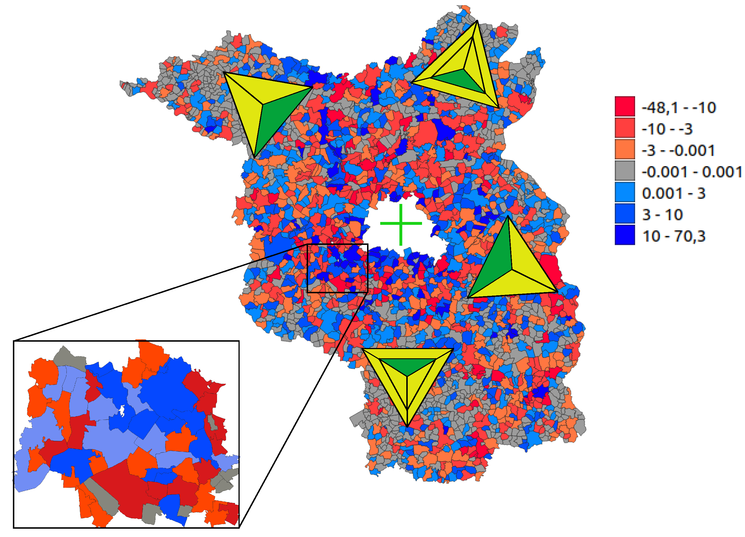
In this section, we apply our approach to the evolution of land prices in Brandenburg, Germany. In general, spatial autoregressive or spatial lag models are widely applied to model housing prices or the evolution of house prices (e.g., Fingleton [34], Osland [35], Baltagi et al. [36], Baltagi et al. [37], Jin and Lee [38]). Furthermore, Taşpınar et al. [39] showed that there are spatial interactions in the volatility of house-price returns. Below, we focus on the spatial dependence structure due to the specifics of the studied area. The state of Brandenburg, with 2370 districts, completely surrounds Berlin. Berlin does not belong to Brandenburg and is therefore not included in the dataset. It is to be expected that the distance to Berlin has a strong influence on the evolution of Brandenburg’s sales prices. It is also to be expected that the influences the districts have on each other is stronger in the vicinity of Berlin.

We consider the sales prices of land that was sold as building land for the first time. The dataset contains the sales prices from 2005 to 2014 for the 2370 districts of Brandenburg. To model the evolution of the sales prices, we take the average prices per square metre for all regions between 2005 and 2009 and compute the difference from the average price for the regions from 2010 to 2014. For regions that do not have sufficient data, we replace the difference in selling price with zero, that is, we assume no price changes between these periods. The resulting map is plotted in Figure 6, on the right.

We wish to investigate whether the districts in the dataset exert a short-distance influence on each other, whether this influence is directional, and in which direction the influence flows. Therefore, we choose the setting such that our weights ${\varphi }_{ij}$ are oriented towards Berlin (similarly to a compass pointing north, hence in Figure 6 the green pieces are pointing to Berlin). Furthermore, we include the following regressors: (1) the distance to Berlin for each district, (2) the squared distance to Berlin, (3) the inverse distance to Berlin, and (4) an intercept of 1. To find the optimal number of directions k and the best length l, we calculate the $K\times L$${\tilde{\mathbf{W}}}_{ij}$ for a subset of $n_0=58$ of the $n=2370$ districts to lower the required computational effort (see Figure 6, left).

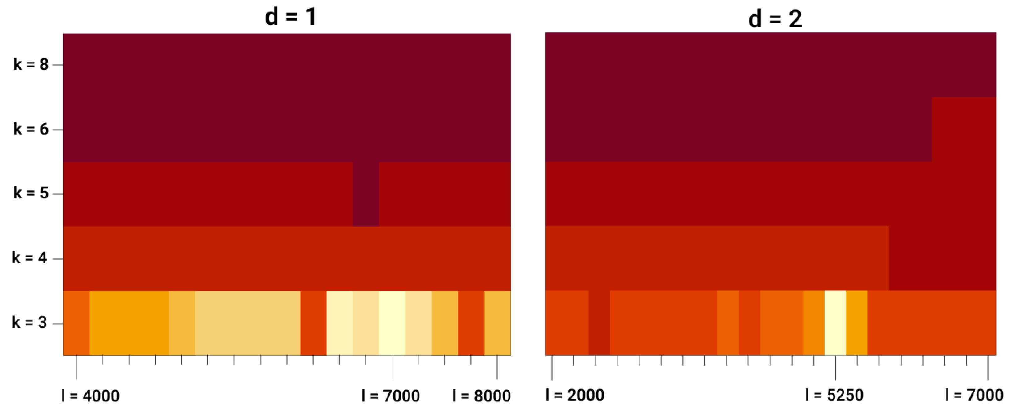
The results of the spatial partitioning are plotted in Figure 7 for distances $d=1$ and $d=2$. In both cases, the best number of directions is $\tilde{k}=3$. In the case where $d=1$, the optimal length of the pieces is $\tilde{l}=7000$ m, and in the case where $d=2$, it is $\tilde{l}=5250$ m. The global best choice, according to the AIC, is the latter setting. For the selection of the optimal length we use step sizes of $\delta l=250$ m.

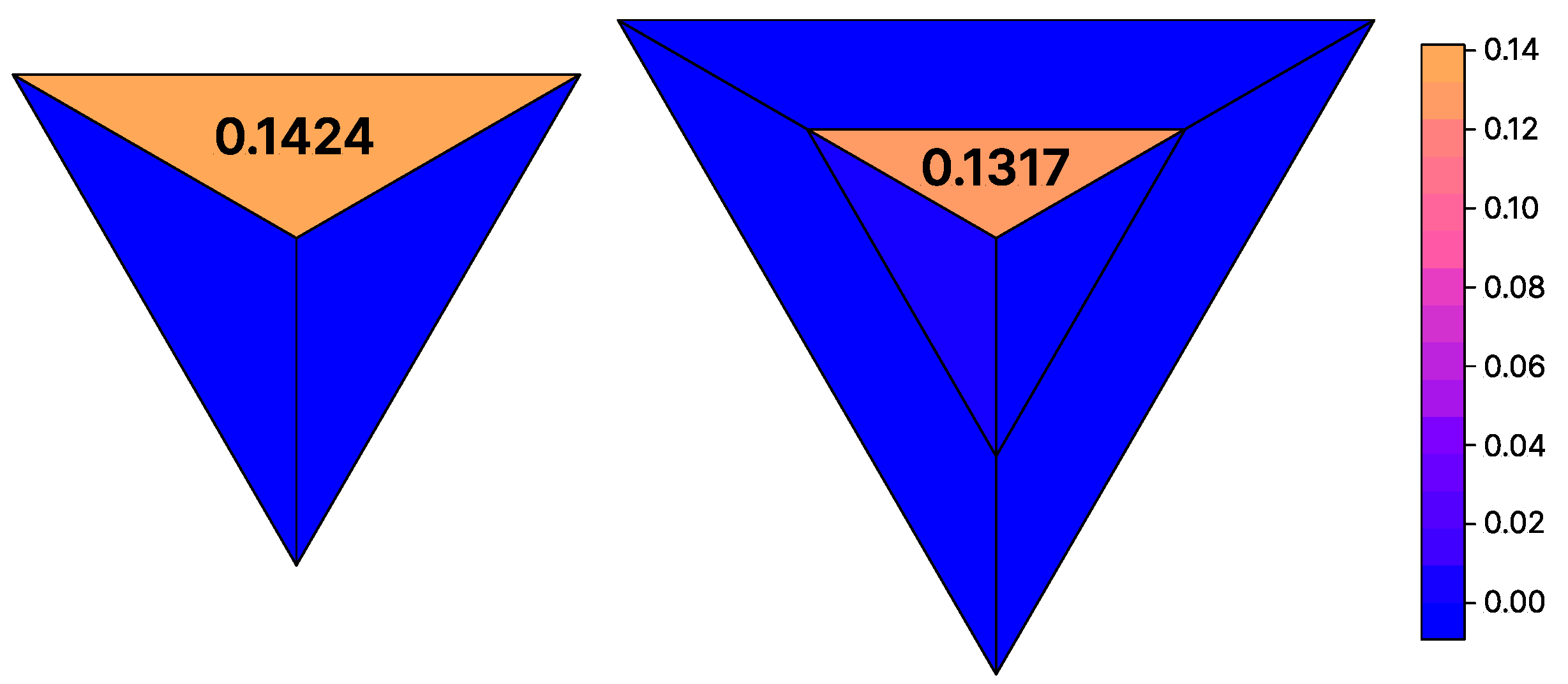
With the optimal settings, we estimated the parameters for $\widehat{\mathbf{\beta }}$ and ${\widehat{\varphi }}_{ij}$ as described in Section 2. We estimated the model $d\times k+p$ times and, after each step, removed the least significant parameter. Finally, we selected the best estimation according to the AIC. In both cases, the estimation with only one parameter was selected via the AIC. In both cases, the remaining parameter is the one pointing towards Berlin (see Figure 8). Furthermore, $\widehat{\mathbf{\beta }}=0$ is selected by our method, which shows that the evolution of the sales prices is not dependent on the distance to Berlin. The result from the real-world study shows that the evolution of the sales prices can be described by a directional influence within the districts of Brandenburg, coming mainly from Berlin.

5. Discussion

Spatial weights matrices for SAR models are of interest in many areas, e.g., for the description of environmental processes such as air pollution or the description of the evolution of housing prices. Numerous methods have therefore been introduced to estimate the spatial weights matrix. However, methods applicable in asymmetric scenarios are lacking.

In this paper, we presented a method for calculating the $n\times n$ spatial weights matrix $\mathbf{W}$ for directional processes which can be symmetric as well as anti-symmetric. The directional influence is assumed to be the same in all regions of a map and is described by the value of the segments ${\varphi }_{ij}$. The proposed method can be used to estimate the directional influence in certain use-cases, such as in the modelling of $P{M}_{2.5}$ in a windy area (see Zhou et al. [22]). In other areas of application, spatial models are created in different environmental areas such as regions of ocean currents (mostly from the same direction). To date, the models have only allowed a symmetric influence or it was necessary to bias the directional influence by knowingly setting certain directions of influence to zero.

In Section 3, we presented Monte Carlo simulations to show that we can re-estimate the ${\widehat{\varphi }}_{ij}$ consistently. Additionally, we showed that weight matrices calculated with our method outperformed a Queen’s contiguity matrix and an inverse-distance weighting matrix in the selection of four directional settings.

In Section 4, we applied our method to real-world data and showed that there is a short-distance influence in the evolution of land sales prices in Brandenburg, Germany. This directional influence flows from Berlin, at the centre of Brandenburg.

One limitation of the proposed method is that the effort required to calculate the overlapping areas of all pizza-like shapes for all regions is computationally demanding. For larger numbers of regions or larger d and k, the proposed method needs to be improved.

In future work, we intend to decrease the computational effort required to calculate the weights matrices $W_{ij}$, to allow a larger number of distances d for the segment shapes. With this in hand, one could investigate whether another means of selecting parameters—other than the AIC—could boost the results, since selection using the AIC always promotes fewer parameters. This could be achieved by predicting which area of which region overlap needs to be calculated. Another suggestion is to try different segment shapes. In this paper, we considered only a pizza-like slicing. It could also be worth investigating whether the estimation itself could be enhanced by using a lasso technique.