
Micromagnetic Simulation of Saturation Magnetization of Nanocrystalline Soft Magnetic Alloys under High-Frequency Excitation

Abstract
:1. Introduction
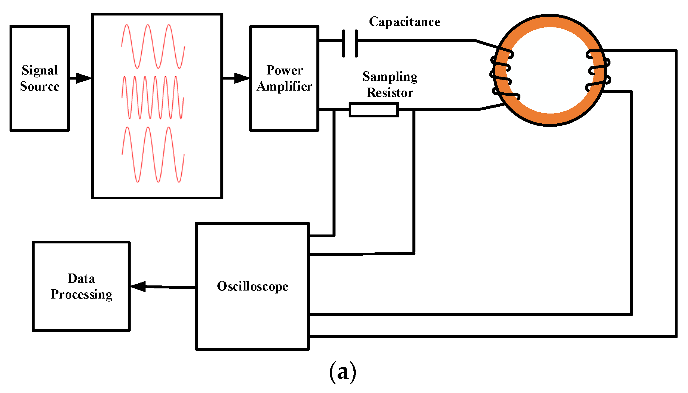
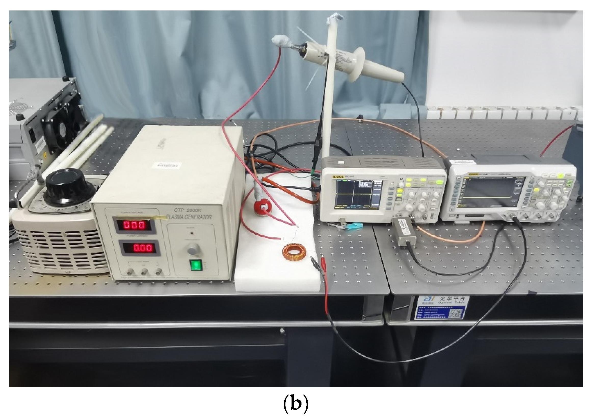
2. Micromagnetic Simulation
2.1. Micromagnetic Simulation Model
- (1)
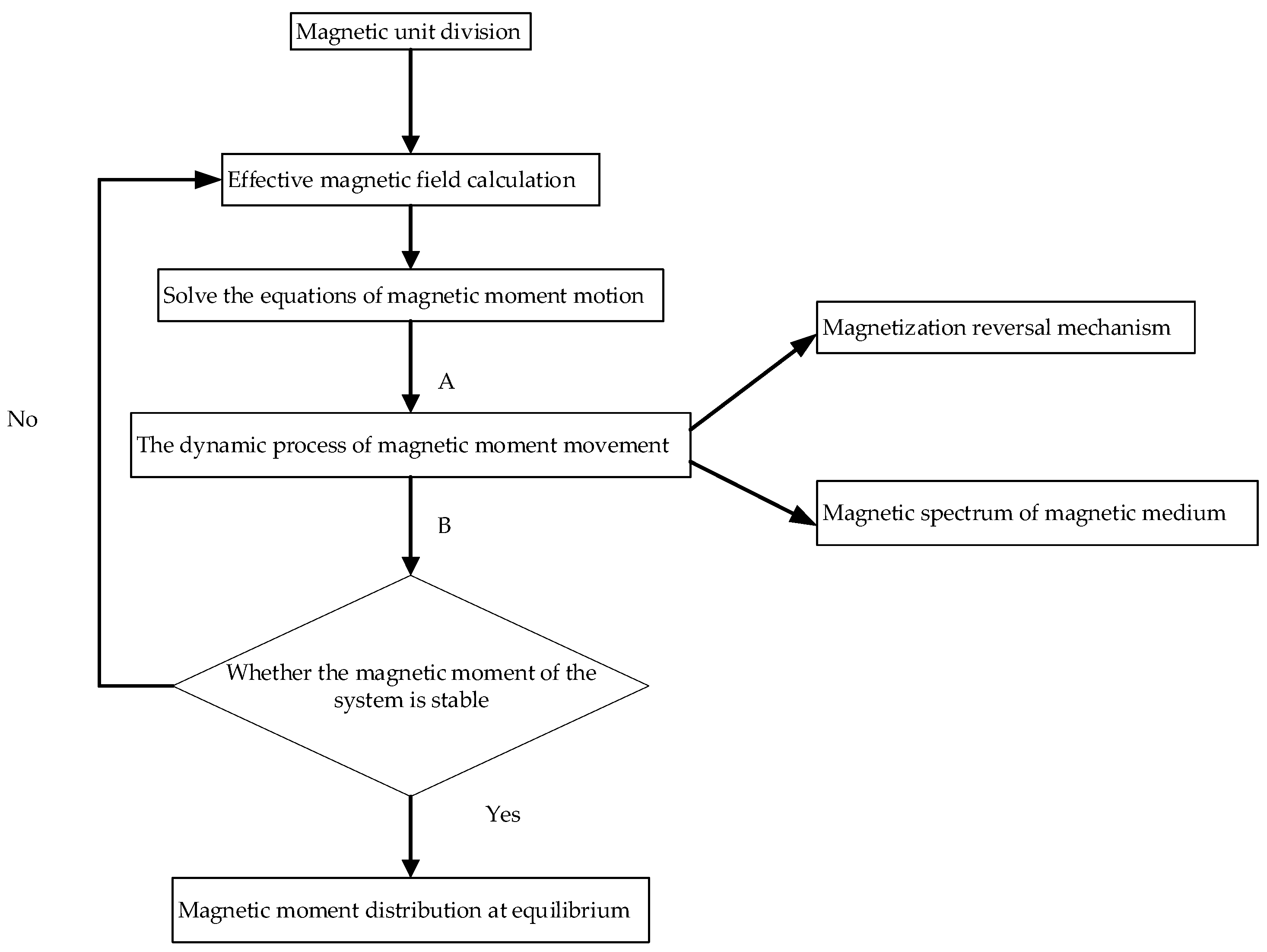
- Determine the simulation system. That is, to determine the shape and size of alloy samples to be studied, and according to the actual material system, correctly set the magnetic model with the property parameters, such as saturation strength, exchange constants, magneto-crystal anisotropy constants, etc.
- (2)
- Magnetic unit division. The microcosmic mesoscopic model can take individual particles as basic or select the collection of magnetic particles.
- (3)
- Effective magnetic field calculation. That is, the equivalent magnetic field acting on each element magnetization vector is calculated according to the magnetic environment of the magnetic medium and all magnetic-related energy terms in the material. Under the excitation of this effective magnetic field, the precession of the magnetization vector follows the LLG equation. If we want to know the dynamic evolution process of the magnetic moment, we can solve this dynamic equation to achieve it.
- (4)
- Process A represents dynamic simulation, which is studying the response characteristics of a magnetic moment in a magnetic system to external field.
- (5)
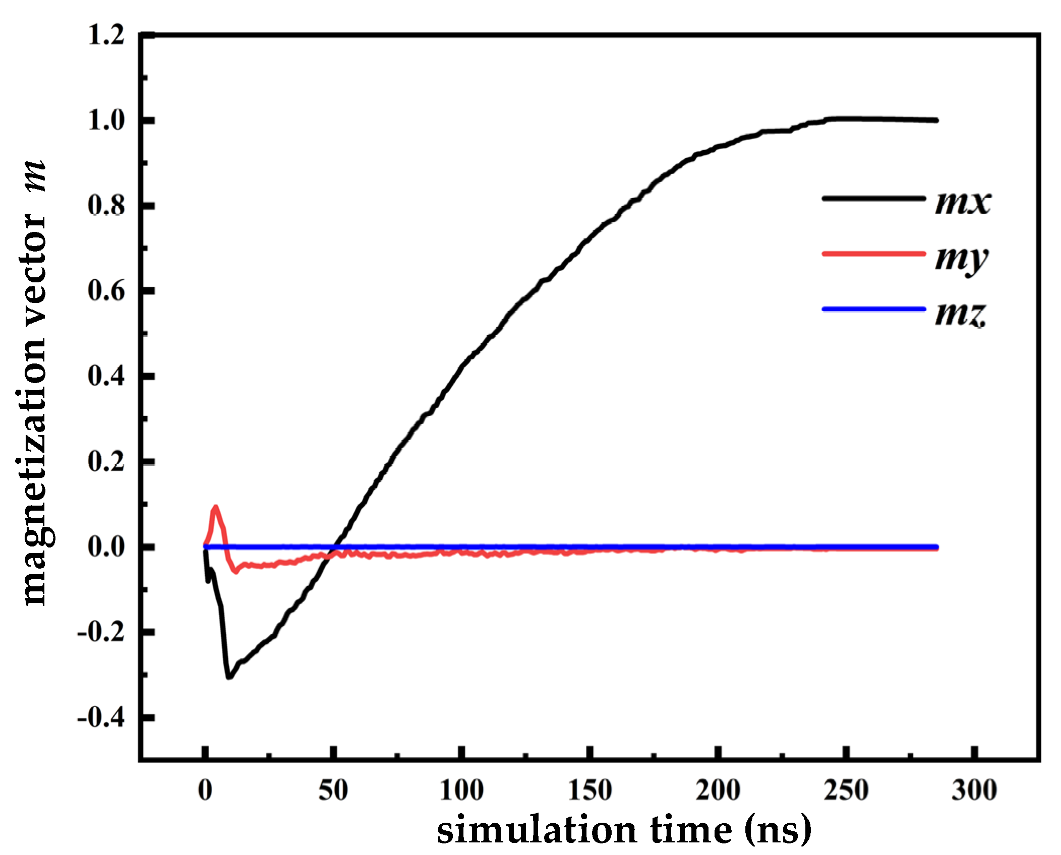
- Process B represents static simulation. That is, studying the magnetic moment distribution of the magnetic system in a stable state. This process can be completed by solving the stable solution of LLG equation.
- (6)
- Check procedure (i.e., MIF document) for unreasonable place, submit procedure.
- (1)
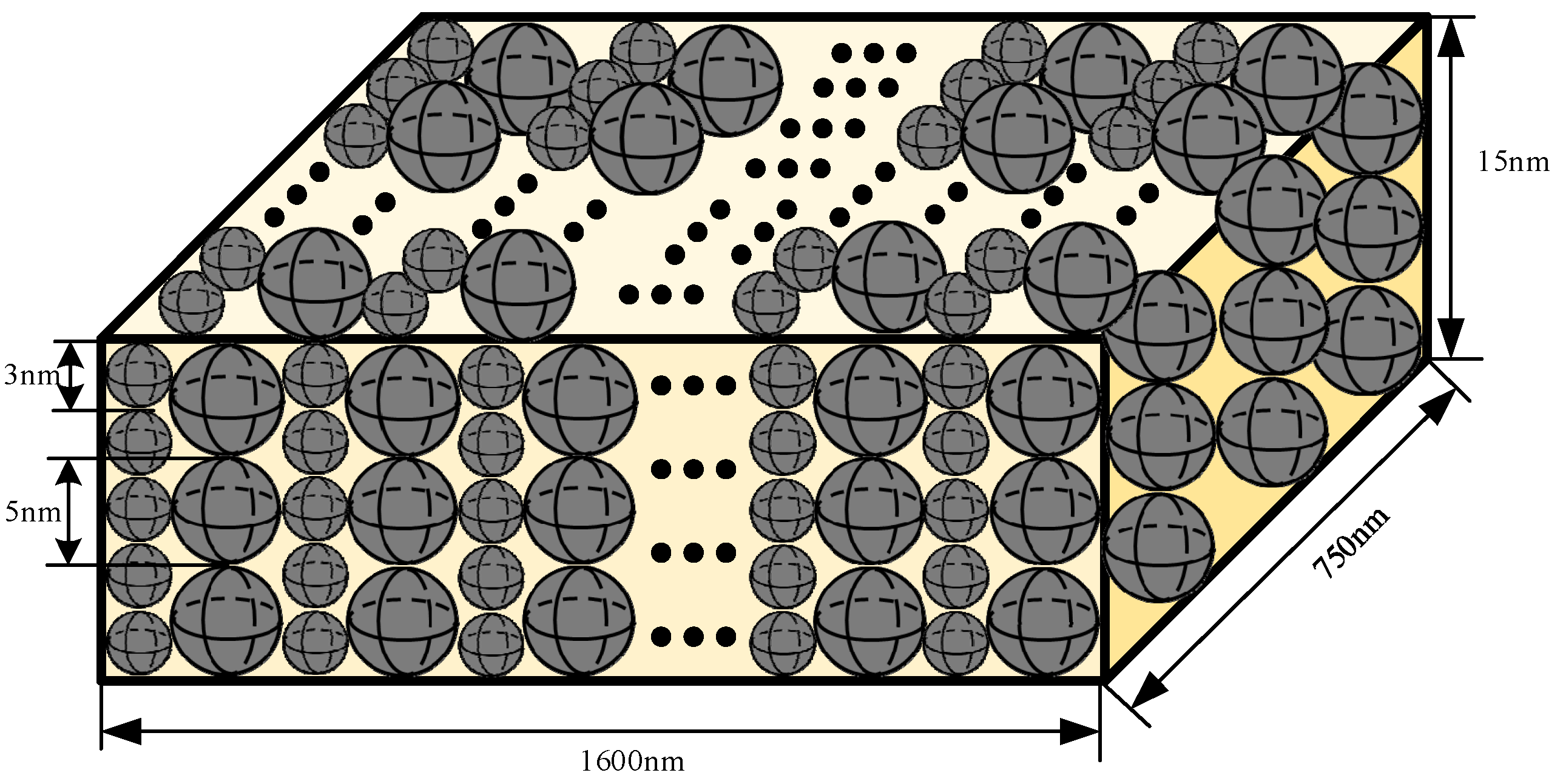
- The magneto-crystalline anisotropy constant of the residual amorphous phase is considered to be zero because it contains no crystal structure.
- (2)
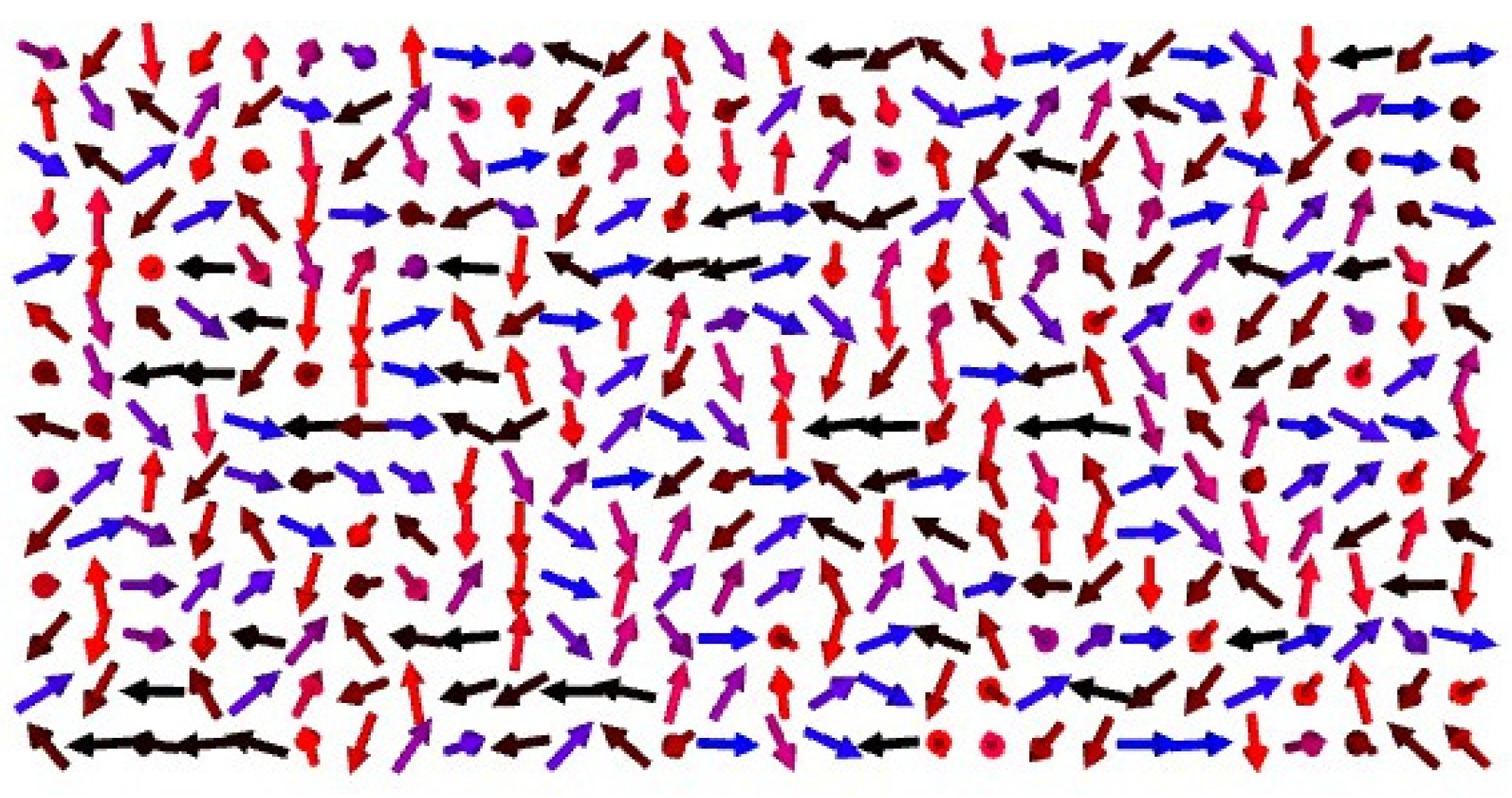
- In the agglomerated phase, spherical nanocrystals are uniformly embedded in the residual amorphous phase, and the ferromagnetic exchange between the nanocrystals is realized through the coupling of the amorphous phase.
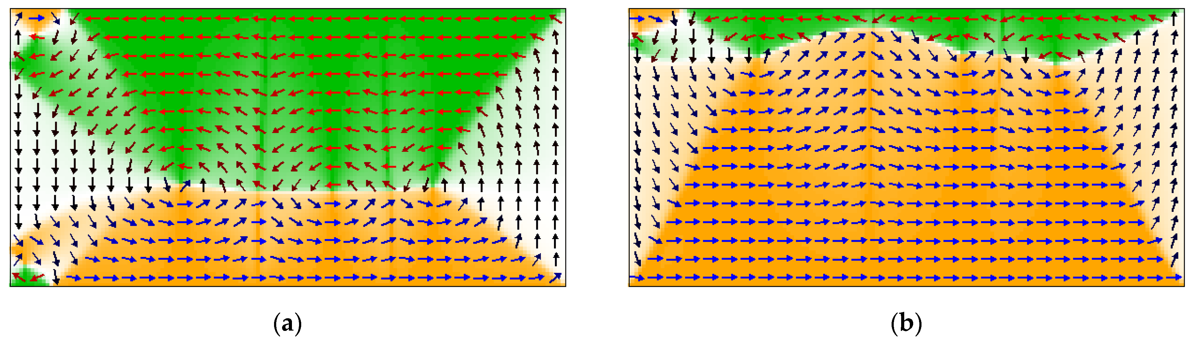
- (3)
- In order to minimize the energy of the magnetic system, the grains in the model tend to be arranged in parallel.
2.2. Model Static Characteristic Parameter Calculation
3. Saturation Magnetization Parameter
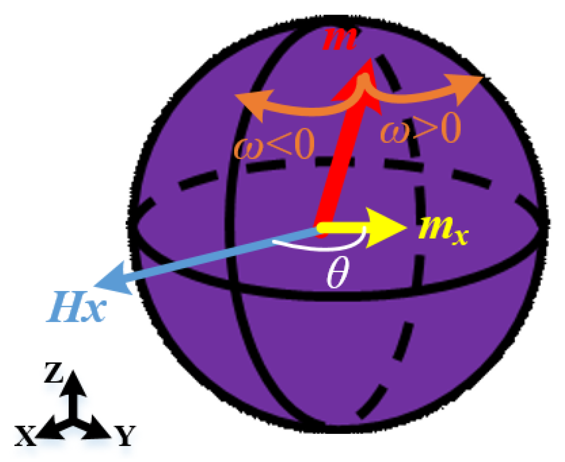
3.1. Magnetic Moment Deflects Angular Velocity
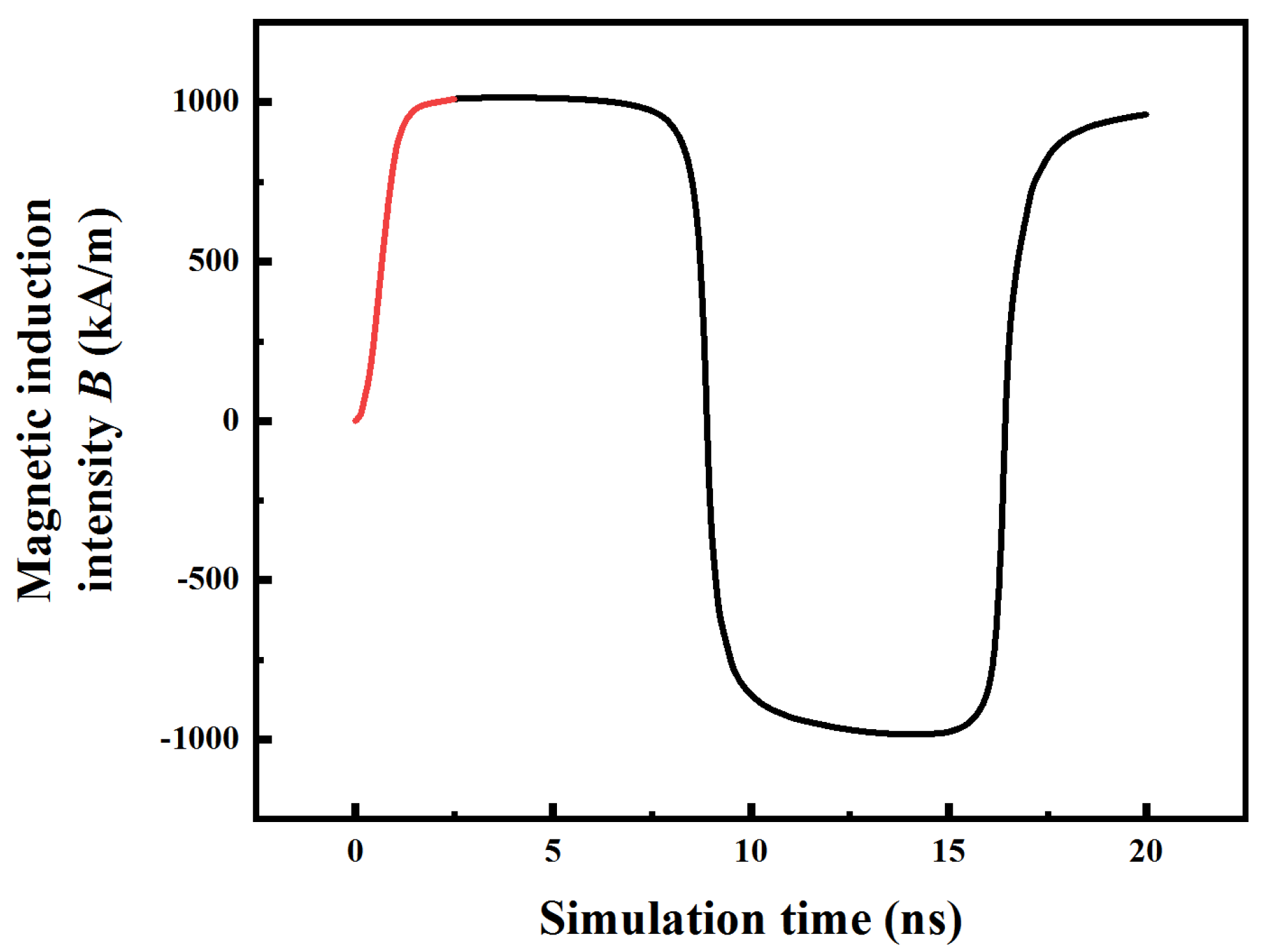
3.2. Magnetization Rate
4. Influence of Alternating Magnetic Field on the Magnetization Process
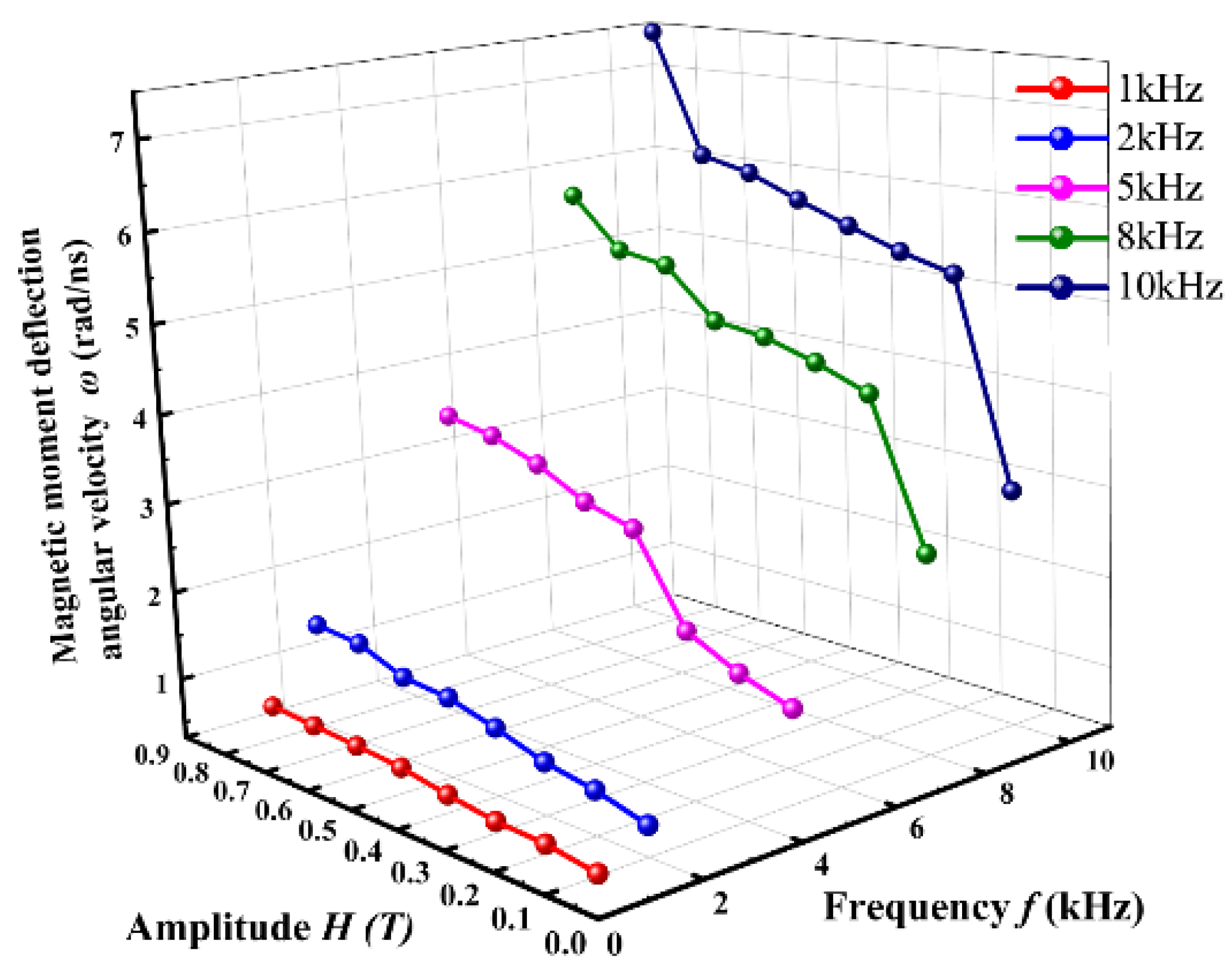
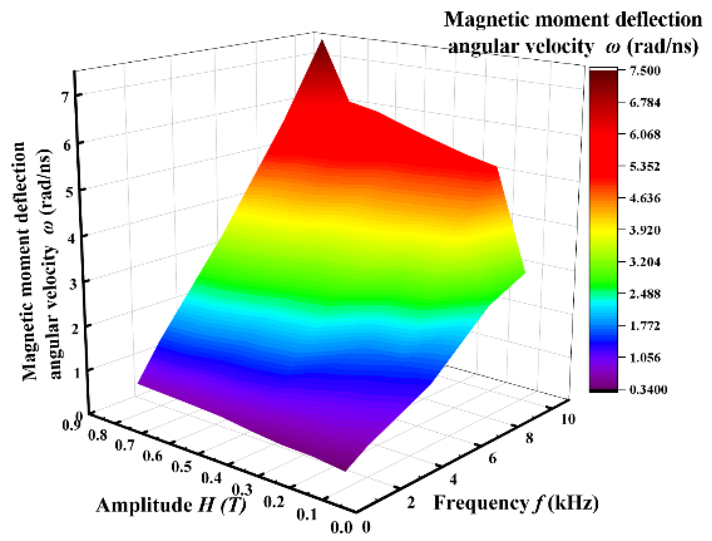
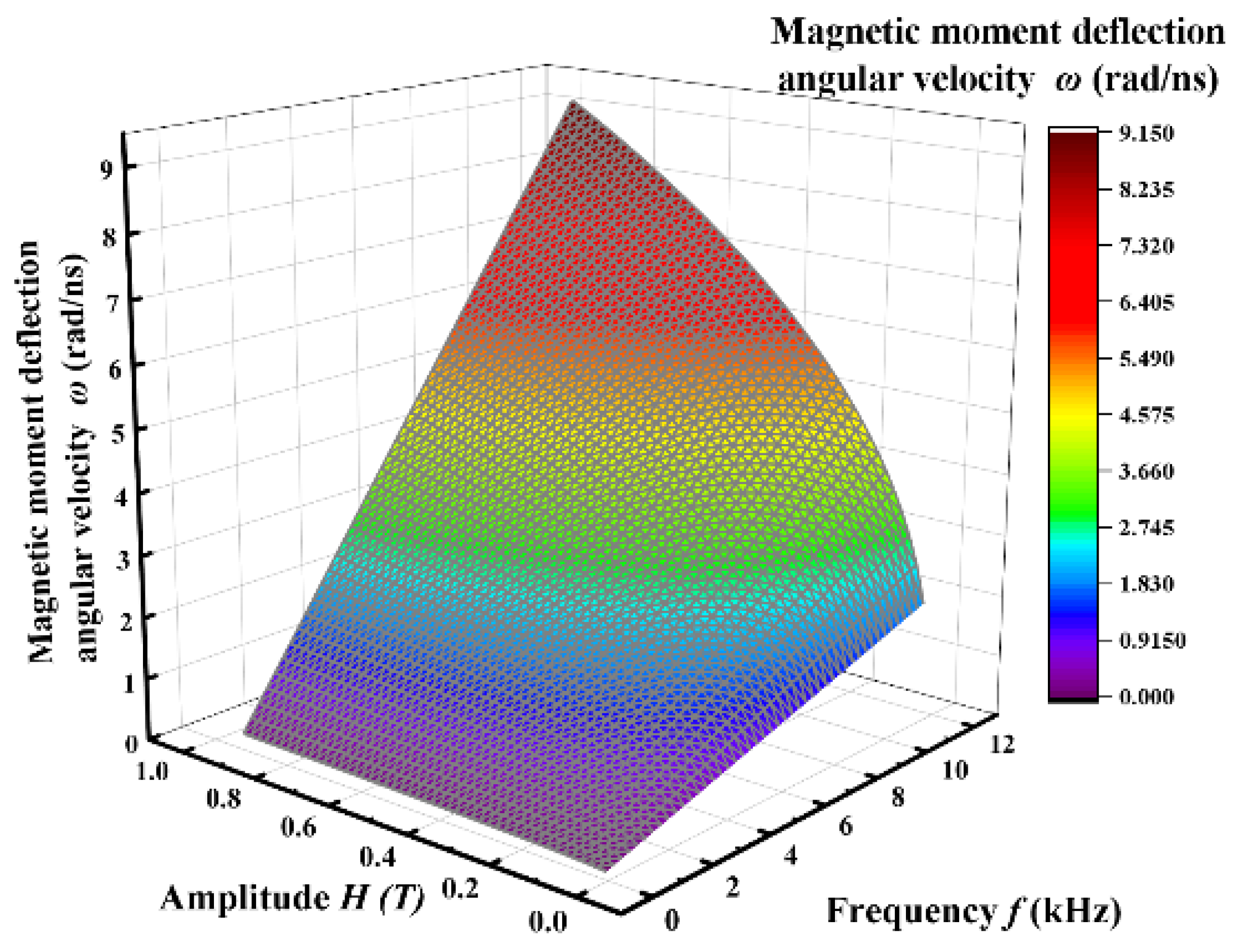
4.1. Influence of Alternating Magnetic Fields on ω
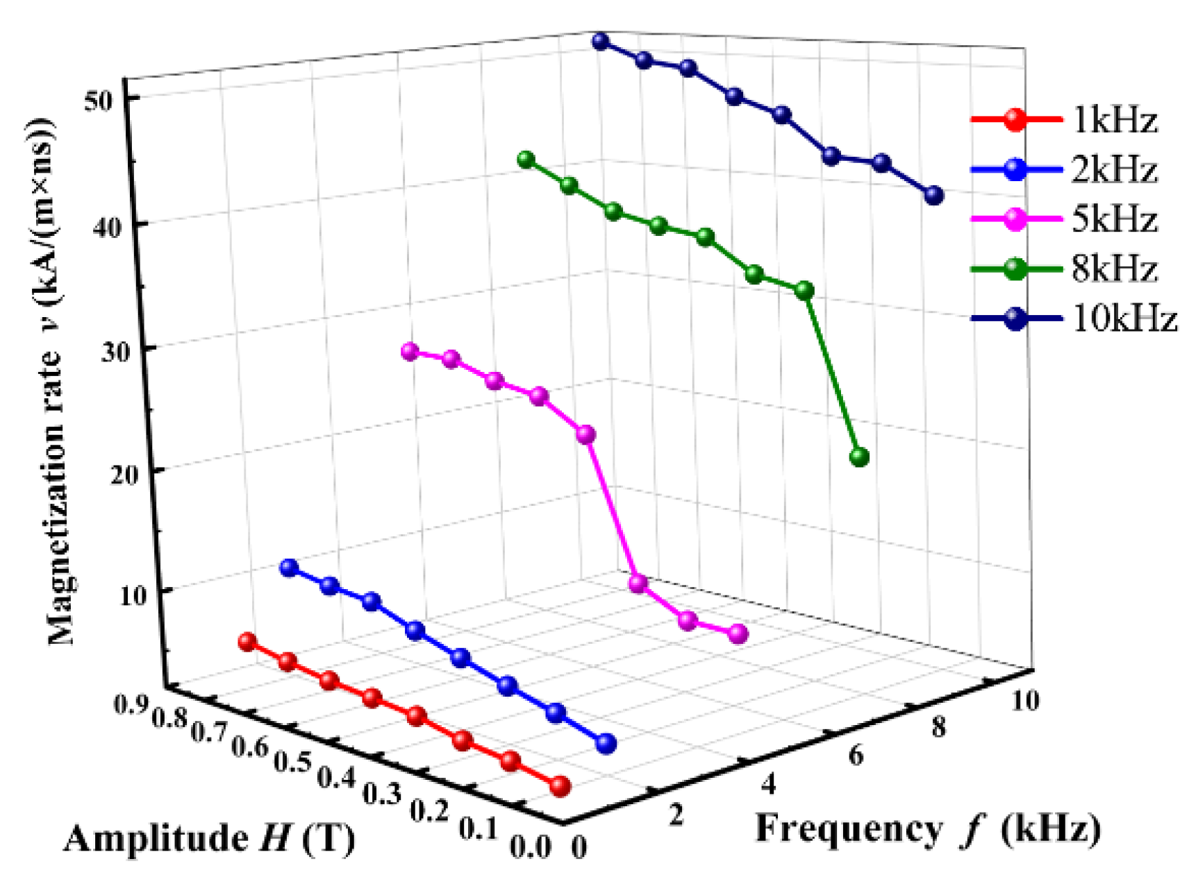
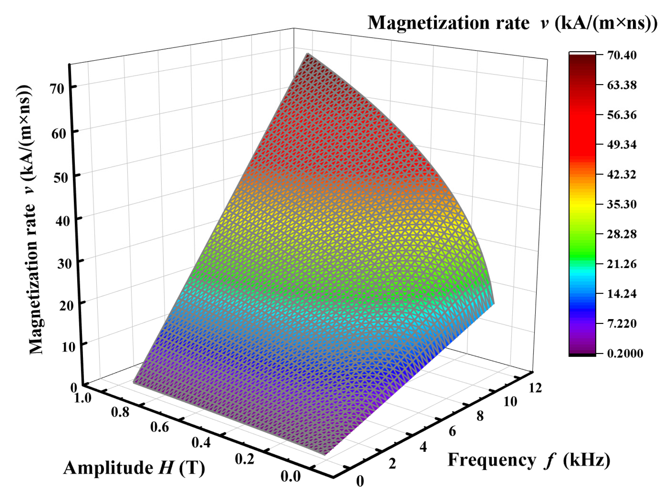
4.2. Influence of Alternating Magnetic Fields on v
5. Conclusions
- (1)
- For the magnetic moment deflection angular velocity ω, ω is positively correlated with f and H. Moreover, when the f of the alternating magnetic field increases gradually, the increasing effect of ω is particularly significant. This is because the size of the effective magnetic field is closely related to the force of magnetic moment deflection. Under the excitation of the standard sine wave, the higher the frequency, the smaller the period and the alternating magnetic field can reach the peak in a relatively short time. Therefore, the increase in frequency has a particularly significant effect on the increase in ω.
- (2)
- For the magnetization rate v, similar to the magnetic moment deflection angular velocity ω, the magnetization rate v is positively correlated with f and H, and when the frequency f of the alternating magnetic field increases gradually, the effect of increasing magnetization rate v is particularly significant. This is because changes in the external working conditions lead to changes in the internal magnetic moment deflection of the material when it is magnetized, which is macroscopically manifested as changes in the overall magnetic induction intensity of the material, thus changing the magnetization rate v.
- (3)
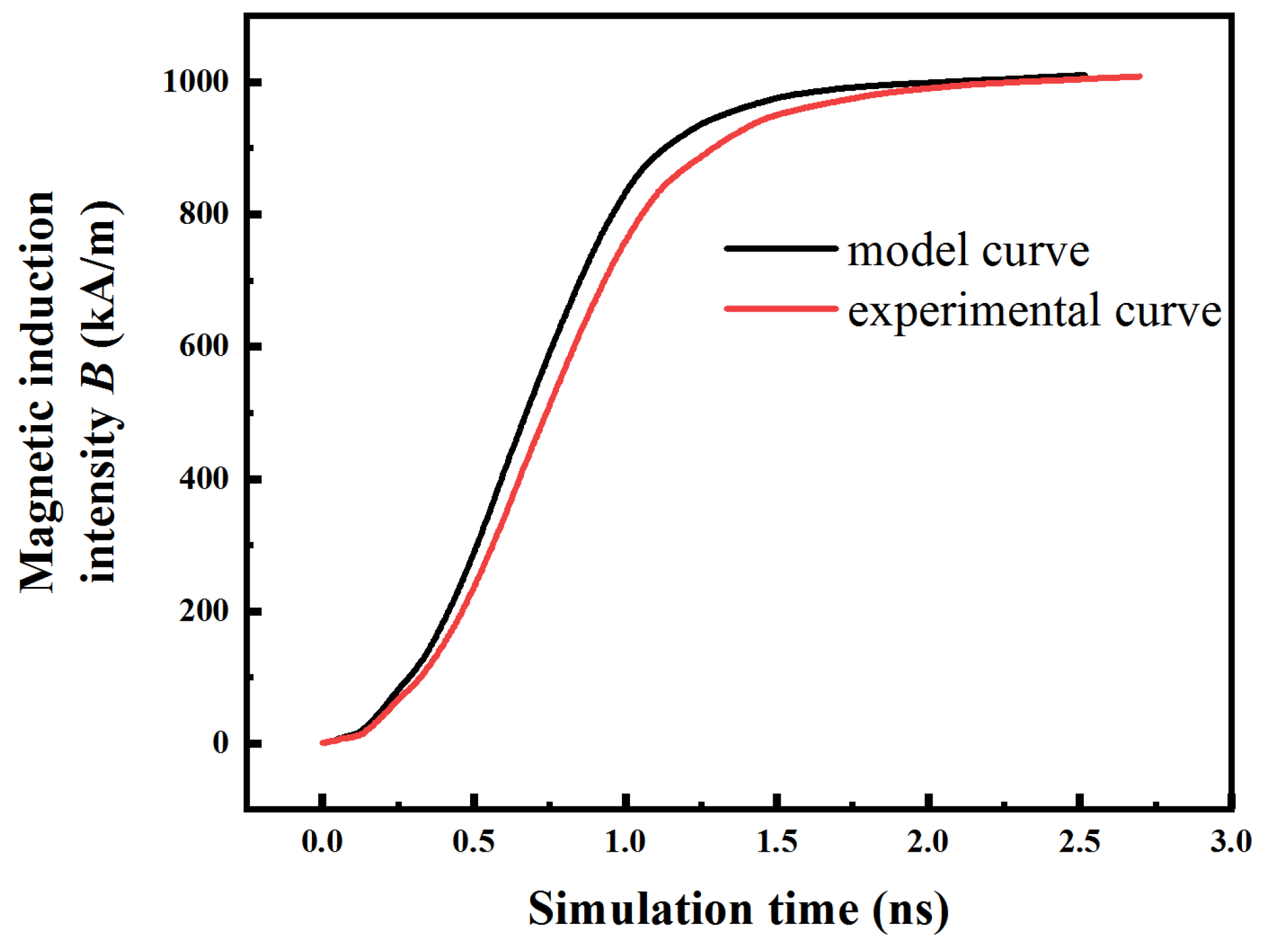
- The fitting toolbox of MATLAB is used to fit the simulation data and the functional relations between ω, v and the alternating magnetic fields f and H are obtained. In the function relation between ω, v and the alternating magnetic field, the coefficient of f is much larger than the coefficient of H. Among them, the coefficient of f in the function relation between ω and f and H is about 2.5 times that of H. The coefficient of f in the functional relationship between v and f and H is about 2.75 times that of H. Multiples of the two are approximately the same, with a relative error of only 9.1%, and the error is analyzed. In addition, the verification between micro and macro is realized.
Author Contributions
Funding
Institutional Review Board Statement
Informed Consent Statement
Data Availability Statement
Conflicts of Interest
References
- Liu, C.; Inoue, A.; Kong, F.L.; Zanaeva, E.; Bazlov, A.; Churyumov, A.; Zhu, S.L.; Al-Marzouki, F.; Shull, R.D. Fe-B-Si-C-Cu amorphous and nanocrystalline alloys with ultrahigh hardness and enhanced soft magnetic properties. J. Non-Cryst. Solids 2021, 554, 68–72. [Google Scholar] [CrossRef]
- Jia, X.; Zhang, B. Direct synthesis of Fe-Si-B-C[sbnd]Cu nanocrystalline alloys with superior soft magnetic properties and ductile by melt-spinning. J. Mater. Sci. Technol. 2022, 108, 186–195. [Google Scholar] [CrossRef]
- Guo, F.; Zhang, T. Mechanisms of hydrides’ nucleation and the effect of hydrogen pressure induced driving force on de-/hydrogenation kinetics of Mg-based nanocrystalline alloys. Int. J. Hydrog. Energy 2022, 47, 1063–1075. [Google Scholar] [CrossRef]
- Zhang, Z.; Liu, X. Effect of Hydrogenation on the Glass Formation Ability and Magnetic Properties of the Fe79Si9B6Nb5Cu1 Amorphous Nanocrystalline Alloys. J. Supercond. Nov. Magn. 2022, 35, 935–940. [Google Scholar] [CrossRef]
- Li, Y.; Jia, X.; Zhang, W.; Zhang, Y.; Xie, G.; Qiu, Z.; Jiao, Z. Formation and crystallization behavior of Fe-based amorphous precursors with pre-existing α-Fe nanoparticles—Structure and magnetic properties of high-Cu-content Fe-Si-B-Cu-Nb nanocrystalline alloys. J. Mater. Sci. Technol. 2021, 65, 171–181. [Google Scholar] [CrossRef]
- Zhang, C. Three-Dimensional Magnetic Properties Measurement and Electromagnetic Finite Element Simulation of Coupled Hysteresis and Anisotropy for Electrical Soft Magnetic Materials; Hebei University of Technology: Tianjin, China, 2016. [Google Scholar]
- Zhi, Q.Z.; Dong, B.S.; Chen, W.Z.; He, K.Y. Elevated temperature initial permeability study of Fe73.5Cu1Nb3Si13.5B9 alloy. Mater. Sci. Eng. 2007, A448, 249–252. [Google Scholar] [CrossRef]
- Wu, J. Micromagnetic Analysis of Mesoscopic High-Frequency Saturation Mechanism of Nanocrystalline Alloys. Master’s Thesis, Shandong University, Jinan, China, 2018. [Google Scholar]
- Han, Z.; Zou, L.; Wu, J.; Zhang, L.; Zhao, T. Micromagnetic analysis of influence of external and internal factors on saturation magnetization of Nanocrystalline alloys at kHz level. Trans. China Electron. Tech. Soc. 2019, 34, 1589–1598. [Google Scholar]
- Flourentzou, N.; Agelidis, V.G.; Demetriades, G.D. VSC-based HVDC power transmission systems: An overview. IEEE Trans. Power Electron. 2009, 24I, 592–602. [Google Scholar] [CrossRef]
- Kenzelmann, S.; Rufer, A.; Dujic, D.; Canales, F.; De Novaes, Y.R. Isolated DC/DC structure based on modular multilevel converter. IEEE Trans. Power Electron. 2015, 30, 89–98. [Google Scholar] [CrossRef]
- Schöbinger, M.; Schöberl, J.; Hollaus, K. Multiscale FEM for the Linear 2-D/1-D Problem of Eddy Currents in Thin Iron Sheets. IEEE Trans. Magn. 2019, 55, 7400212. [Google Scholar] [CrossRef]
- Kim, M.K.; Sim, J. Dynamical Origin of Highly Efficient Energy Dissipation in Soft Magnetic Nanoparticles for Magnetic Hyperthermia Applications. Phys. Rev. Appl. 2018, 9, 054037. [Google Scholar] [CrossRef]
- Lekdim, A.; Morel, L.; Raulet, M.A. Effect of the remaining magnetization on the thermal ageing of high permeability nanocrystalline FeCuNbSiB alloys. J. Magn. Magn. Mater. 2006, 460, 125–128. [Google Scholar] [CrossRef]
- Liu, D.; Zhao, T.; Zhang, M.; Wang, L.; Xi, J.; Shen, B.; Sun, J. Exploration of nontrivial topological domain structures in the equilibrium state of magnetic nanodisks. J. Mater. Sci. 2021, 56, 4677–4685. [Google Scholar] [CrossRef]
- Herzer, G. Modern soft magnets: Amorphous and nanocrystalline materials. Acta Mater. 2013, 61, 718–734. [Google Scholar] [CrossRef]


| Magnetic Parameter | Nanocrystalline Phase | Residual Amorphous Phase |
|---|---|---|
| The coefficient of exchange A (J/m) | 1 × 10⁻¹¹ | 6 × 10⁻¹² |
| Magneto-crystalline anisotropy constant K1 (J/m3) | 8 × 10² | 0 |
| Saturation magnetization Ms (T) | 1.31 | 1.16 |
| Hs (kA/m) | Bs (T) | Hc (A/m) | |
|---|---|---|---|
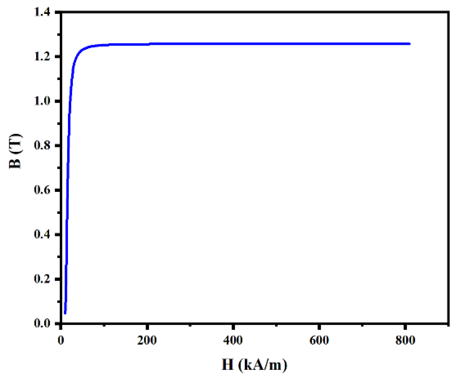
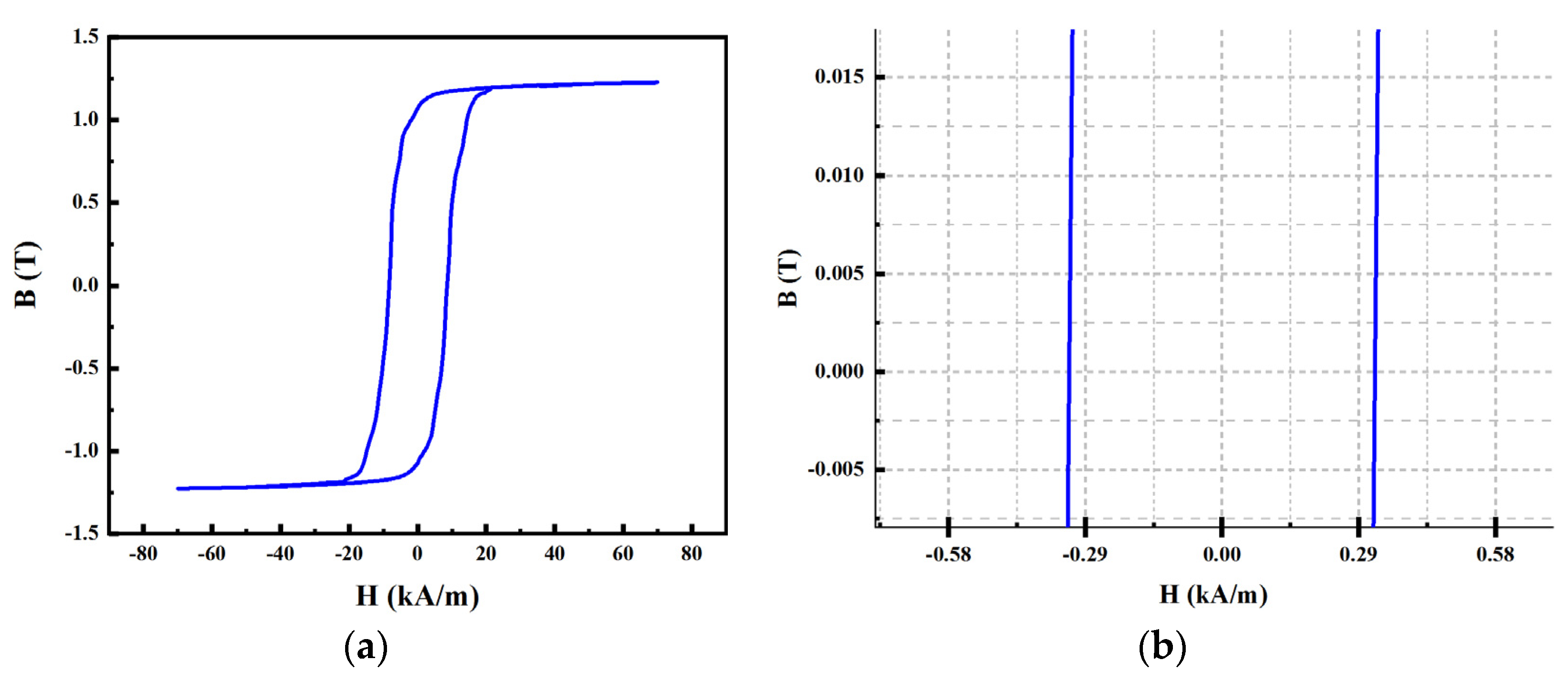
| Computational data | 220 | 1.247 | 307 |
| Experimental data | 225 | 1.24 | 310 |
| Amplitude H (T) | Magnetic Moment Deflection Angular Velocity ω (rad/ns) | ||||
|---|---|---|---|---|---|
| 1 kHz | 2 kHz | 5 kHz | 8 kHz | 10 kHz | |
| 0.1 | 0.32 | 0.66 | 1.35 | 2.54 | 2.95 |
| 0.2 | 0.43 | 0.81 | 1.54 | 4.13 | 5.2 |
| 0.3 | 0.45 | 0.9 | 1.82 | 4.35 | 5.35 |
| 0.4 | 0.52 | 1.07 | 2.78 | 4.52 | 5.55 |
| 0.5 | 0.61 | 1.21 | 2.93 | 4.59 | 5.76 |
| 0.6 | 0.65 | 1.25 | 3.21 | 5.12 | 5.99 |
| 0.7 | 0.68 | 1.45 | 3.4 | 5.2 | 6.12 |
| 0.8 | 0.73 | 1.49 | 3.5 | 5.75 | 7.5 |
| Amplitude H (T) | Magnetization Rate v (kA/(m×ns)) | ||||
|---|---|---|---|---|---|
| 1 kHz | 2 kHz | 5 kHz | 8 kHz | 10 kHz | |
| 0.1 | 2.31 | 4.41 | 9.73 | 20.97 | 40.25 |
| 0.2 | 2.98 | 5.58 | 9.77 | 33.45 | 42.45 |
| 0.3 | 3.37 | 6.57 | 11.75 | 34.24 | 42.69 |
| 0.4 | 4.14 | 7.70 | 22.84 | 36.78 | 45.76 |
| 0.5 | 4.46 | 8.84 | 25.23 | 37.28 | 47.02 |
| 0.6 | 4.75 | 10.20 | 25.84 | 38.06 | 49.17 |
| 0.7 | 5.24 | 10.55 | 27.02 | 39.87 | 49.64 |
| 0.8 | 5.86 | 11.14 | 27.07 | 41.74 | 51.09 |
Publisher’s Note: MDPI stays neutral with regard to jurisdictional claims in published maps and institutional affiliations. |
© 2022 by the authors. Licensee MDPI, Basel, Switzerland. This article is an open access article distributed under the terms and conditions of the Creative Commons Attribution (CC BY) license (https://creativecommons.org/licenses/by/4.0/).
Share and Cite
Guo, K.; Zou, L.; Dai, L.; Zhang, L. Micromagnetic Simulation of Saturation Magnetization of Nanocrystalline Soft Magnetic Alloys under High-Frequency Excitation. Symmetry 2022, 14, 1443. https://doi.org/10.3390/sym14071443
Guo K, Zou L, Dai L, Zhang L. Micromagnetic Simulation of Saturation Magnetization of Nanocrystalline Soft Magnetic Alloys under High-Frequency Excitation. Symmetry. 2022; 14(7):1443. https://doi.org/10.3390/sym14071443
Chicago/Turabian StyleGuo, Kaihang, Liang Zou, Lingjun Dai, and Li Zhang. 2022. "Micromagnetic Simulation of Saturation Magnetization of Nanocrystalline Soft Magnetic Alloys under High-Frequency Excitation" Symmetry 14, no. 7: 1443. https://doi.org/10.3390/sym14071443